
 Submit a Paper
 Propose a Special lssue
 Open Access
ARTICLE
Prediction and Comparative Analysis of Rooftop PV Solar Energy Efficiency Considering Indoor and Outdoor Parameters under Real Climate Conditions Factors with Machine Learning Model
1 Copernicus Institute of Sustainable Development, Utrecht University, Princetonlaan 8A, Utrecht, 3584 CB, The Netherlands
2 Computer Engineering Department, Igdir University, Igdir, 76000, Turkiye
3 Electronical and Electronic Engineering Department, Engineering Faculty, Bitlis Eren University, Bitlis, 13100, Turkiye
* Corresponding Author: Gökhan Şahin. Email:
(This article belongs to the Special Issue: Advanced Artificial Intelligence and Machine Learning Methods Applied to Energy Systems)
Computer Modeling in Engineering & Sciences 2025, 143(1), 1215-1248. https://doi.org/10.32604/cmes.2025.063193
Received 08 January 2025; Accepted 20 March 2025; Issue published 11 April 2025
 View Full Text
 Download PDF
Abstract
This research investigates the influence of indoor and outdoor factors on photovoltaic (PV) power generation at Utrecht University to accurately predict PV system performance by identifying critical impact factors and improving renewable energy efficiency. To predict plant efficiency, nineteen variables are analyzed, consisting of nine indoor photovoltaic panel characteristics (Open Circuit Voltage (Voc), Short Circuit Current (Isc), Maximum Power (Pmpp), Maximum Voltage (Umpp), Maximum Current (Impp), Filling Factor (FF), Parallel Resistance (Rp), Series Resistance (Rs), Module Temperature) and ten environmental factors (Air Temperature, Air Humidity, Dew Point, Air Pressure, Irradiation, Irradiation Propagation, Wind Speed, Wind Speed Propagation, Wind Direction, Wind Direction Propagation). This study provides a new perspective not previously addressed in the literature. In this study, different machine learning methods such as Multilayer Perceptron (MLP), Multivariate Adaptive Regression Spline (MARS), Multiple Linear Regression (MLR), and Random Forest (RF) models are used to predict power values using data from installed PV panels. Panel values obtained under real field conditions were used to train the models, and the results were compared. The Multilayer Perceptron (MLP) model was achieved with the highest classification accuracy of 0.990%. The machine learning models used for solar energy forecasting show high performance and produce results close to actual values. Models like Multi-Layer Perceptron (MLP) and Random Forest (RF) can be used in diverse locations based on load demand.Keywords
Solar energy is a highly promising renewable energy source, capable of fulfilling a substantial fraction of global energy requirements [1]. Effective exploitation of this energy necessitates careful measurement of solar insolation on Earth and a correct estimate of the resultant data. The intensity of solar insolation influences both the types of products produced and is vital for numerous agricultural and meteorological uses [2]. Traditionally, non-electronic sensors were employed in meteorological observation stations to quantify insolation intensity, a crucial metric of solar energy. This change enhanced data quality but also introduced issues, including the necessity for qualified workers and elevated operational costs, leading to difficulty in acquiring long-term insolation intensity data.
To address these challenges and provide access to historical insolation intensity data for planning, numerous predictive models have been created utilizing diverse methodologies. The models encompass artificial neural networks, time series techniques, physical radiative transfer models, and stochastic weather methods [3]. These models generally forecast insolation intensity by employing diverse data as input parameters, with meteorological data being one of the most commonly used inputs worldwide [4]. Regression approaches are frequently utilized in these models to forecast insolation intensity based on inputs such as temperature, relative humidity, cloud cover, and sunshine duration. Numerous scholars have specifically analyzed the correlation between historical maximum and minimum temperature data and insolation intensity [5–7].
Recently, researchers have increasingly utilized artificial intelligence methodologies, including Artificial Neural Networks (ANN), Adaptive Neuro-Fuzzy Inference Systems (ANFIS), Genetic Programming (GP), and Support Vector Machines (SVM), alongside conventional regression methods to predict insolation intensity [8]. Numerous studies have utilized artificial intelligence techniques to forecast insolation intensity, producing encouraging outcomes. A study calculated insolation intensity by utilizing the daily maximum and minimum temperature readings from four meteorological stations in the Basque region of Northern Spain from 1999 to 2003 [9]. The Gene Expression Programming (GEP) approach was employed, and the outcomes were juxtaposed with other artificial intelligence methods (ANN, ANFIS) and empirical equations. The research indicated that AI techniques were more effective in assessing insolation intensity, with the GEP method surpassing ANN and ANFIS.
Another study determined insolation intensity utilizing the traditional Angström-Prescott equation, which establishes a linear correlation between solar radiation and sunshine duration [10]. Nevertheless, variable weather conditions cause fluctuations in energy derived from solar radiation, requiring the storage of surplus energy for subsequent utilization [11]. The efficient storage and subsequent utilization of renewable energy depend significantly on precise forecasting, with numerous studies concentrating on solar energy prediction through weather data, statistical methods, and machine learning techniques. Solar energy predictions can be conducted for both short-term and long-term periods [12]. In recent years, many studies have focused on the application of deep learning in renewable energy. Studies by [13,14] support this claim.
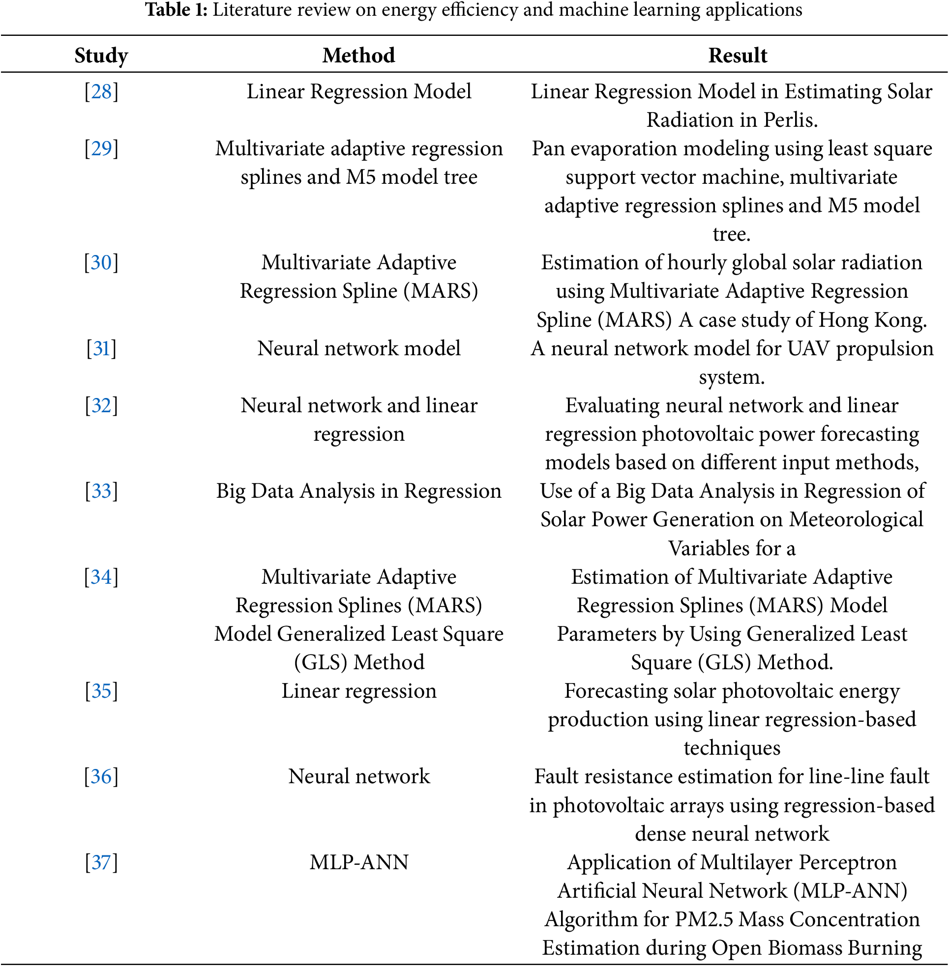
In 2014, the American Meteorological Society (AMS) conducted a competition on Kaggle to determine the most effective statistical and machine-learning techniques for short-term solar energy forecasting. The competition sought to forecast total daily solar energy at 98 Oklahoma Mesonet locations. Meteorological data was obtained from 144 Global Ensemble Forecast Systems (GEFS) across the United States [15]. Numerous research employing the AMS dataset have been undertaken since that time. Shahid et al. employed Ridge Regression and Random Forest algorithms, attaining Mean Absolute Error (MAE) values of 22.84 and 22.75, respectively [14]. Díaz-Vico et al. achieved a Mean Absolute Error (MAE) of 2.56 using Deep Convolutional Neural Networks (DCNN) [16]. Various studies have shown differing MAE values employing distinct methodologies, hence underscoring the efficacy of machine learning techniques in solar energy forecasting [12,15,17]. Furthermore, research has explored the utilization of artificial intelligence techniques including Random Forest Regression (RFR), Gradient Boosted Regression (GBR), and Extreme Gradient Boosting (XGB) for both global and local wind energy forecasting, in addition to solar radiation prediction [18,19]. These investigations have consistently demonstrated that AI methodologies surpass conventional regression techniques in forecasting insolation intensity. In a study, Nematirad and Pahwa employed a Bayesian-optimized multilayer perceptron (MLP) and artificial neural network (ANN) to forecast solar radiation, attaining mean absolute error (MAE) values of 109.45 and 111.24, respectively, when Pearson correlation coefficients (PCC) were utilized [20–22]. A subsequent work formulated a novel Angström equation that enhances the conventional model, markedly decreasing error rates in both short-term and long-term predictions [23,24]. The suggested model incorporated two novel dependence coefficients and outperformed the standard Angström equation in forecasting insolation intensity utilizing meteorological data from 163 sites in Turkey. Three solar irradiation locations in Turkey were evaluated for their solar energy potential utilizing the HarLin model, which integrates harmonic and classical regression techniques. The HarLin model surpassed the ANFIS and Angstrom-Prescott methods in forecasting insolation energy potential [25]. In Algeria, daily and monthly insolation intensity was assessed using a Support Vector Machine (SVM) in conjunction with meteorological information, with an Adaptive Neuro-Fuzzy Inference System (ANFIS) marginally surpassing other methodologies according to the criteria of percentage of prediction residuals (POPR), R2, and Mean Absolute Error (MAE) [26]. In five nations, Decision Tree (DT) regression algorithms were employed to forecast insolation intensity, demonstrating performance on par with ANN and SVM, underscoring the model’s potential [27]. Hourly insolation intensity was assessed utilizing Support Vector Regression (SVR), ANN, and DT methodologies, all yielding satisfactory forecasts based on POPR and R2 [13]. This research distinguishes itself from prior studies by employing both indoor parameters namely Open Circuit Voltage (Voc), Short Circuit Current (Isc), Maximum Power (Pmpp), Maximum Voltage (Umpp), Maximum Current (Impp), Fill Factor (FF), Parallel Resistance (Rp), Series Resistance (Rs), and Module Temperature and outdoor parameters including Air Temperature, Humidity, Dew Point, Air Pressure, Irradiation, Wind Speed, and Wind Direction—as input data. We utilized two machine learning methodologies, Multi-Layer Perceptron’s (MLP) and Random Forest (RF), to forecast the energy output of the Photovoltaic Outdoor Test Plant (UPOT) at Utrecht University. The integration of both indoor and outdoor parameters, an aspect often overlooked in other studies, allows for a more comprehensive analysis, capturing the complex interplay of factors influencing PV panel efficiency in real-world conditions. The efficiency of photovoltaic panels is affected by several factors, including light-induced degradation, temperature-induced degradation, oxygen and humidity-induced degradation, and ion migration. Photovoltaic devices have self-healing capabilities, restoring deterioration overnight upon exposure to light. This study examines the efficacy of novel solar module layouts and their performance under various indoor and outdoor environments. The objective is to improve our comprehension of these aspects by assessing specific energy yields (energy rating) in kWh/kWp in both indoor and outdoor environments. The results seek to enhance photovoltaic system efficacy. Furthermore, Table 1 in the manuscript encapsulates several machine learning methodologies employed in diverse facets of solar energy efficiency as derived from the current literature.
This study is organized as follows: Section 2 provides a detailed overview of the materials and methods used to obtain the research findings. Section 3 and 4 offers a thorough review of the results, accompanied by a comprehensive discussion. Lastly, Section 5 presents a conclusive summary of the study.
Study Area
The Utrecht region (Fig. 1) experiences warm, partially overcast summers and long, extremely cold, windy, and predominantly cloudy winters. Temperatures fluctuate between 0°C and 22°C, never falling below −6°C or surpassing 28°C. Cloud cover exhibits seasonal variation, with July representing the month of greatest clarity (56% of the sky clear or partly cloudy). December experiences the greatest frequency of precipitation, averaging 9.9 days. Rain constitutes the predominant kind of precipitation, reaching a zenith of 34% on 22 December. The duration of daylight varies from 7 h and 44 min in December to 16 h and 45 min in June. Humidity comfort levels stay rather consistent throughout the year. Wind velocities peak from October to April, averaging in excess of 18.1 km/h. June is the month with the highest solar radiation, averaging 6.3 kWh. The area’s geography is predominantly flat, featuring a maximum elevation variation of 25 m and an average altitude of 4 m above sea level.

Figure 1: Utrecht/Netherland province Location map (Latitude: 52.0907374, Longitude: 5.1214201) [38]
This section defines the variables and explains the data collection methodology. It then describes different machine learning methods such as Multilayer Perceptron (MLP), Multivariate Adaptive Regression Spline (MARS), Multiple Linear Regression (MLR), and Random Forest (RF) models, along with their configuration details. Fig. 2 illustrates the overall research workflow, including data collection, preprocessing, model training, evaluation, and final efficiency prediction.

Figure 2: Overview of the research methodology and workflow
The methods used to train and validate the models, data pre-processing, and evaluation techniques are also specified. Model performance is assessed using the metrics shown in Fig. 3. The values corresponding to each characteristic are presented in Table 2.

Figure 3: The Utrecht University Photovoltaic Outdoor Test (UPOT) facility measures the real-world performance of various commercial and prototype PV modules [38]
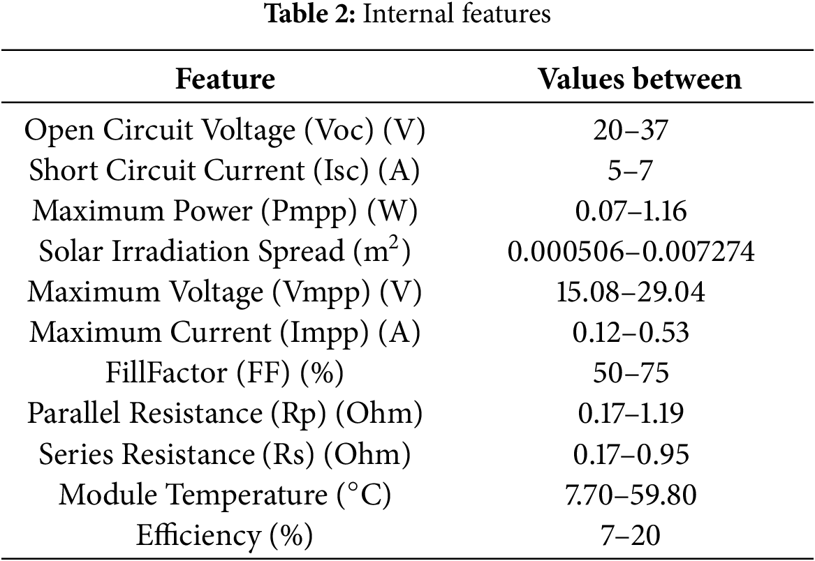
2.1 Variables Used for PV Solar Power Plant Efficiency
The efficiency of a photovoltaic system is defined as the ratio of total power produced (kWh/year) to the total global solar radiation received (kWh/year). It is affected by both ambient (outside) and modular (interior) factors:
Outdoor Parameters
Solar Irradiation (W/m2): Intensity of sunlight received. Higher levels increase electricity generation.
Air Temperature (°C): Affects efficiency; higher temperatures usually decrease performance.
Wind Speed (m/s): Enhances heat dissipation, improving performance.
Relative Humidity (g/m3): Influences dust accumulation on panels.
Air Pressure (millibars): Affects panel structural integrity but not efficiency directly.
Dew Point: Temperature at which water vapor condenses.
Wind Speed Spread: Wind speed spread denotes the fluctuation and dispersion of wind velocities over a temporal framework. Intense winds are seldom, although moderate to strong winds are more prevalent. The Weibull distribution, utilized for modeling wind speed distribution, is asymmetrical and defined by shape and scale factors. This distribution aids in optimizing turbine design and minimizing expenses.
Wind Direction and Spread: The direction of the wind influences turbine positioning, as turbines diminish wind energy for downstream locations. Turbines should be oriented to align with the prevailing wind direction to optimize efficiency. The design must account for the proximity to the grid and the dimensions of the property to reduce expenses. Locations with a distinct prevailing wind direction facilitate closer turbine installation, maximizing land utilization and reducing infrastructure expenses.
Indoor Parameters
Module Power (kW): Maximum electrical output.
Module Temperature (°C): Higher temperatures can reduce output.
Open Circuit Voltage (Voc): Maximum voltage when not connected to a circuit.
Short Circuit Current (Isc): Current when two points with different voltages touch.
Maximum Power (Pmpp), Voltage (Umpp), and Current (Impp): Key performance indicators.
Fill Factor (FF): Ratio of maximum power to the product of Voc and Isc.
Parallel Resistance (Rp) and Series Resistance (Rs): Affect current flow and efficiency.
Module Efficiency: Module efficiency is the ratio of generated electricity to incoming solar energy. It indicates how effectively a PV system converts sunlight into electrical power.
The Utrecht University Photovoltaic Outdoor Test Facility (UPOT) collected data every 5 min to assess the real-world performance of different PV modules. Solar radiation was measured using a pyranometer (Kipp & Zonen CMP11), with an uncertainty of approximately ±5%, caused by calibration errors and environmental factors.
PV Panel Data: Daily measurements of panel characteristics, including temperature and power, were recorded over a year to observe long-term trends.
Historical Weather Data: To assess the impact of weather on PV performance, historical data and PV module parameters (e.g., Open Circuit Voltage, Short Circuit Current) were collected for the same location. This included environmental factors such as air temperature, humidity, dew point, air pressure, and wind conditions.
Data Validation: Measures were taken to ensure data accuracy by addressing outliers, inconsistencies, and missing values.
Data Organization: The data were systematically organized and stored for effective analysis.
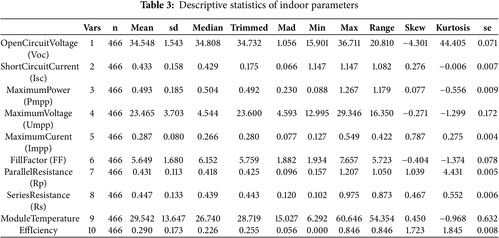
2.3 Statistical Analysis of the Dataset
Tables 3 and 4 present the statistical summary of the dataset used in our experiments. The tables contain 10 and 11 parameters, respectively. Among these, Efficiency represents the dependent variable predicted at the output, while the remaining parameters are independent variables used as inputs.

2.4 Multi-Layer Perceptrons (MLP) Architecture
This work utilized a Multi-Layer Perceptron (MLP) architecture to model and forecast performance indicators under diverse situations. The MLP, a category of feedforward neural networks, comprises several layers of nodes, including an input layer, one or more hidden layers, and an output layer. Each node, or neuron, in one layer is connected with a certain weight to every node in the subsequent layer, and these connections are modified during training to reduce prediction errors. The architecture of MLPs consists of an input layer that accepts input data, with the number of neurons in this layer corresponding to the number of features in the input dataset. The hidden layers comprise one or more layers where calculations occur, with each layer’s neurons employing an activation function to introduce non-linearity, hence enabling the model to learn intricate patterns. Prevalent activation functions comprise ReLU (Rectified Linear Unit). Ref. [39], sigmoid, and hyperbolic tangent. The output layer generates the final prediction, with the quantity of neurons in this layer aligned with the number of output classes or regression goals. This work constructed the MLPs with different quantities of hidden layers and neurons per layer to assess their performance (Fig. 4). The configurations evaluated comprised structures with three, four, and five layers. Each model was trained by backpropagation to reduce the Mean Absolute Error (MAE), Mean Squared Error (MSE), and Root Mean Squared Error (RMSE), while maximizing the R-squared (R2) value.

Figure 4: 5-layer MLP architecture
The training procedure for the MLP models encompassed multiple stages. Initially, data normalization was conducted to guarantee that feature values were on a comparable scale. Weights were initially allocated using He initialization [40] to prevent problems such as vanishing or expanding gradients. The models were trained utilizing a loss function suitable for regression tasks, namely the mean squared error loss. The Adam optimizer [41] was employed to modify the weights according to the calculated gradients. Furthermore, early stopping was utilized to avert overfitting by observing the validation loss and ceasing training if the loss failed to improve for 5 epochs. Furthermore, early stopping was utilized to avert overfitting by observing the validation loss and ceasing training if the loss failed to improve for 5 epochs. The MLP design has been thoroughly examined and utilized across multiple areas owing to its adaptability and efficacy in modeling nonlinear interactions. The book by [42] offers a comprehensive examination of deep learning methodologies, featuring in-depth analyses of MLP designs and training procedures. Furthermore, Ref. [40] employed a multi-layer perceptron (MLP) architecture to forecast environmental pollution, whereas Ref. [43] utilized this design to anticipate power plant efficiency. Our study seeks to get high accuracy in predictive modeling by utilizing the flexibility and capabilities of MLPs, thereby illustrating the efficacy of deep learning methods in managing intricate datasets.
2.5 Multivariate Adaptive Regression Spline (MARS)
While model estimate with numerous data points typically yields accurate predictions, it may also result in erroneous outcomes [44]. The application of conventional linear models significantly elevates the error rate, particularly in the modeling of nonlinear connections. In this instance, it is more suitable to favor nonlinear models. The MARS model is one of the techniques employed in the development of nonlinear models. This model is a nonparametric regression model [45]. A precise functional pattern between the dependent and independent variables is unnecessary. The methodology was established by [46]. This strategy does not necessitate stringent assumptions like those of a linear regression model [46]. This model attains nonlinearity by estimating piecewise linear regression lines, which involves partitioning the independent variable into smaller segments and calculating distinct regression coefficients for each segment [47]. The many lines produced are interconnected by nodal points. The efficacy of the MARS method in constructing predictive models has been shown in various areas, including intrusion detection, energy price forecasting, cancer diagnosis, software engineering, and credit scoring. This method allows for the inclusion of variables in the model either individually or by the multiplication of several variables.
The basic function is defined as the MARS Eq. (1) [48,49].
where
The MARS method employs a general-to-specific strategy in model construction. Initially, all subdivisions are divided into two sister subdivisions, with the division optimized according to goodness-of-fit criteria. This procedure iterates until a substantial quantity of discrete subdivisions is achieved, each with its corresponding basis function. A model that is overlearned is thus generated. Subsequently, the basis functions that do not substantially enhance the model’s fit are eliminated in reverse order. During pruning, both the model’s accuracy and its complexity are meticulously regulated. The model’s complexity is so diminished [46]. Upon the creation of the MARS model, the relative significance of the independent variables used in the model can be assessed. To do this, all factors associated with the variable whose relative significance is to be assessed are eliminated from the model, and the goodness of fit loss resulting from the variable’s exclusion is computed. The goodness of fit loss is computed for all variables in this manner, assigning each variable a score ranging from 0 to 100. The magnitude of the variable scores signifies their importance [50].
The fundamental functions for linear and non-linear expansion are utilized in two distinct manners. The bidirectional fundamental functions (x − t) + and (t − x) + are represented as the t node value, as delineated in Eqs. (2) and (3). The (+) symbol adjacent to these functions signifies that the outcome of the equation is positive. Alternatively, each function is assessed at the origin [44]. Fig. 5 illustrates a singular node and two fundamental functions. Each function is piecewise linear, with the t value located at the node. These two functions constitute reflected pairs. The fundamental functions are segmented linear regression curves that partition the variables into intervals with optimal junctions. Another objective of MARS is to identify the joints with the minimal sum of squares. In the model’s formation, the forward-stepping approach generates several nodes that contribute minimally or not at all, but these superfluous nodes will be eliminated by the stepwise pruning procedure. Model selection is predicated on the Generalized Cross Validation (GCV) criterion established by references [51]. This coefficient considers both the residual error and the complexity of the model. The GCV coefficient is expressed in the following equation [52].
where n is; the number of sample data, C, measures the cost-complexity of the added basic functions, Yi is the observed value of a response variable,

Figure 5: Basis function
If there are Multiple linear regression independent basic functions in the models are presented as follows [43]:
Adjusted Coefficient of Determination was described by [53]:
Standard Deviation Ratio was defined by by [40,50,54]:
Given that the equation is in linear form, the outcomes of the MARS model are assessed utilizing ANOVA. MARS facilitates the comparison of low- and high-grade models by permitting the specification of variables to be entered either individually or in combination. Reference [55] advocates for the use of corrected R2 as a standard. A model incorporating interaction terms is favored alone if the adjusted R2 is substantially elevated [56].
2.6 Multiple Linear Regression
In the multiple linear regression (MLR) method, the impact of several input parameters (independent variables, predictors) on a single output parameter (dependent variable, response) is analyzed. In this study, seven parameters were used as inputs to the MLR model to estimate the efficiency parameter. The general form of the multiple linear regression equation is given by:
In Eq. (8), Yi represents the dependent variable in the multiple linear regression, Xi’s are the independent variables, d’s are the regression coefficients, and
In Eq. (9),
It enables the creation of diverse models and classifications by training each decision tree on distinct observation samples using multiple decision trees (Fig. 6) [57]. Its user-friendliness and adaptability facilitated its rapid uptake and extensive utilization, as it effectively tackles both classification and regression challenges. The algorithm’s most commendable aspect is its capacity to facilitate a deeper exploration of your cluster by generating many models from your dataset [58,59].

Figure 6: Random forest model architecture
Algorithm: The dataset for analysis is prepared, including the creation of the set and, if necessary, data cleansing. The algorithm generates a decision tree for each sample, and the estimated value outcome of each decision tree is produced. Voting is conducted for each anticipated value. The algorithm ultimately produces a result by choosing the most frequently voted value for the final prediction. It does the analysis methodically.
3 Experimental Setup and Procedures
This study assessed the efficacy of feedforward different machine learning methods such as the Multilayer Perceptron (MLP) model, Multivariate Adaptive Regression Spline (MARS) model, Multiple Linear Regression (MLR) model, and Random Forest (RF) models utilizing data from the Utrecht University Photovoltaic Outdoor Test Facility (UPOT). Prior to inputting the data into the models, a sequence of preparation procedures was executed to guarantee the dataset’s quality and compatibility. The stages encompassed data cleansing, standardization, and partitioning into training and test sets via k-fold cross-validation. The dataset included in the study comprised daily average values from January 2023. A total of 466 samples were collected at five-minute intervals every day from the solar panel, and the dataset was partitioned into training and test sets utilizing k-fold cross-validation with k set to 10. The procedure entailed partitioning the data into 10 segments, utilizing 9 segments for training and 1 segment for testing. The division of training and test sets was conducted ten times to assure result consistency and mitigate randomness. The MLP model utilized nine input features from the module, comprising Open Circuit Voltage (Voc), Short Circuit Current (Isc), Maximum Power (Pmpp), Maximum Voltage (Umpp), Maximum Current (Impp), Fill Factor (FF), Parallel Resistance (Rp), Series Resistance (Rs), and Module Temperature, alongside ten environmental output features, including Air Temperature, Air Humidity, Dew Point, Air Pressure, Irradiation, Irradiation Spread, Wind Speed, Wind Speed Spread, Wind Direction, and Wind Direction Spread, to forecast the efficiency of the photovoltaic (PV) roof solar power plant. The characteristics were standardized to guarantee uniform scaling among variables. The MLP model comprised an input layer with seven neurons, a solitary hidden layer containing 15 neurons, and an output layer with one neuron tasked with forecasting efficiency values. The results indicated that employing 15 neurons in a solitary hidden layer produced the optimal performance (Fig. 4). Nonetheless, increasing the number of hidden layers to two resulted in a deterioration of the network’s performance, signifying a problem of overfitting.
The Random Forest model utilized the identical nine input features and ten output factors to forecast the effectiveness of the photovoltaic roof solar power plant. The dataset underwent preprocessing in a comparable manner, with features standardized for uniformity. In contrast to MLP, the Random Forest model relies on the binary correlations among input and output attributes and the target variable (efficiency). Regression analysis was conducted to estimate continuous numerical values in the output layer.
In both models, the training data were utilized to develop the models, while the test data were applied to assess their predictive efficacy. Multiple performance criteria, such as R-squared (R2), root mean square error (RMSE), mean absolute error (MAE), and mean absolute percentage error (MAPE), were employed to evaluate and compare the efficacy of the MLP and Random Forest models.
This study compares the performance of various models, including Multilayer Perceptrons (MLP), Architecture, Multivariate Adaptive Regression Splines (MARS), Multiple Linear Regression, Training Conditional Inference Trees, and Random Forest, demonstrating the superior efficacy of Multilayer Perceptrons (MLP) in modeling complex relationships regarding solar panel efficiency, yielding better results than other regression methods. The prevalent external factors influencing solar panel efficiency, specifically environmental and inside parameters, are identified and examined. This study aims to investigate the influence of outdoor and indoor conditions on panel power efficiency via machine learning techniques, with the aforementioned metrics employed for comparison. The MLP multilayer sensors model exhibits a R2 value of 0.983 for outdoor parameters and 0.983 for indoor parameters. The multiple linear regression model demonstrates a R2 value of 0.87 for outdoor parameters and 0.901 for indoor parameters. The MARS regression model reveals a R2 value of 0.916 for outdoor parameters and 0.7800244 for indoor parameters. The Random Forest Model demonstrates a R2 value of 0.956 for the outside parameter and a R2 value of 0.9746905 for the inside parameters. The Multiple Linear Regression model exhibits a R2 value of 0.899 for the outside parameter and a R2 value of 0.6979885 for the indoor parameters. The outcomes of the root mean squared error (RMSE), mean absolute error (MAE), and mean absolute percentage error (MAPE) are presented in Tables 4 and 5. The artificial neural network model surpassed the multiple linear regression model by attaining superior outcomes across all evaluation criteria.
4.1 MARS, MLR and RF Model and Interpretation
The graph below illustrates a strong linear link between the Module Temperature variable and both the Fill Factor (FF) and Maximum Voltage (Fig. 7a,b). This may lead to issues in the functioning of numerous machine learning models, particularly MARS [56]. Multicollinearity may lead to the misinterpretation of inconsequential variables as significant. A potential remedy to this issue could involve eliminating highly interactive variables from the model. This issue can be addressed by generating alternative variables through techniques like principal component analysis [44].

Figure 7: Correlation graph of internal and external parameters. (a) Correlation graph of internal parameters. (b) Correlation graph of external parameters
To prevent overfitting in data mining models, datasets are typically divided into training and test sets for result validation. The training, testing, and regression curves of the Random Forest (RF) model for all data are illustrated in Fig. 8. The models developed from the training set are evaluated with the test set in the final phase, therefore minimizing model bias. Nevertheless, the data set must have a sufficient number of observations to employ this strategy. Seventy percent is allocated to training, while thirty percent is designated for testing. The 5-repetition 10-fold method was used as the cross-validation technique to ascertain the optimal fine-tuning value. The optimal sub-model was identified as the one with the highest cross-validation R2 value. This section analyzes the goodness of fit criteria of the models, revealing that the most effective model for both the training and test sets is the random forest. Upon examining all the models, specifically the Multi-Layer Perceptron (MLP) model and the Random Forest (RF) model. The performance disparity between the training and test sets suggests that the model is experiencing overfitting. Consequently, the generalization of the model poses challenges. The performance disparity between the training and test sets (Tables 6 and 7) suggests that the model is experiencing overfitting. Nevertheless, for all models, even if the disparity is not as pronounced as that reported in RF, the same issue persists.

Figure 8: Regression curve fitting of (a) training, (b) test and (c) all data for the RF


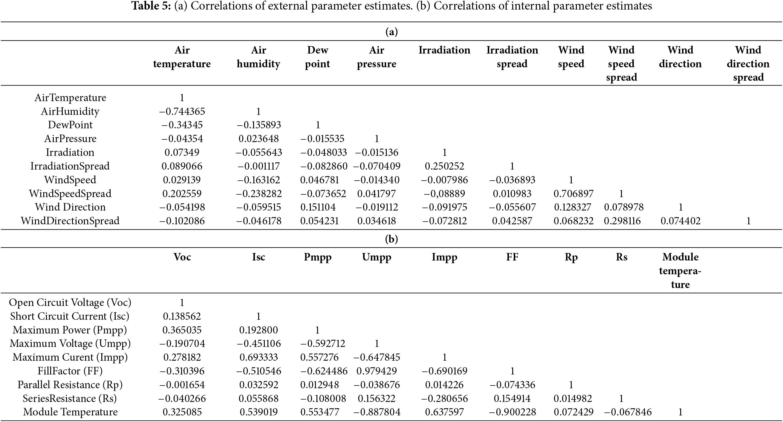
The correlations presented in Table 5 illustrate the distinct impact of internal and exterior characteristics on panel efficiency through the subsequent calculations. This formula is derived from the Random Forest model. These relationships are illustrated in Fig. 9.


Figure 9: Variables with strong correlations with PV solar power efficiency. (a) Effect of open circuit on PV panel efficiency. (b) Effect of short circuit on PV panel efficiency. (c) Effect of maximum power on PV panel efficiency. (d) Effect of maximum voltage on PV panel efficiency. (e) Effect of maximum current on PV panel efficiency. (f) Effect of fill factor on PV panel efficiency. (g) Effect of parallel resistance on PV panel efficiency. (h) Effect of series resistance on PV panel efficiency
To prevent overfitting in data mining models, datasets are typically divided into training and test sets for result validation. The models developed from the training set are evaluated with the test set in the final phase, therefore minimizing model bias. Nevertheless, the data set must have a sufficient number of observations to employ this strategy. Seventy percent is allocated for training, while thirty percent is designated for testing. This section compares Conditional Inference Trees, Random Forests, MARS, and Linear Regression techniques. The caret package was utilized to train the models. The 5-repetition 10-fold method was used as the cross-validation technique to ascertain the optimal fine-tuning value. The optimal sub-model was identified as the one with the highest cross-validation R2 value. This section analyzes the goodness of fit criteria of the models, revealing that the most effective model for both the training and test sets is the random forest. Upon examining all the models, specifically the Multi-Layer Perceptron (MLP), Multivariate Adaptive Regression Splines (MARS), Multiple Linear Regression (MLR), Conditional Inference Trees (CIT), Linear Regression (LR), and Random Forest (RF) models. The performance disparity between the training and test sets suggests that the model is experiencing overfitting. Consequently, the generalization of the model is troublesome. Nevertheless, the MARS model, regarded as the second most effective model, had superior performance in cross-validation, as the results for the test and training sets were closely aligned. Furthermore, it is important to highlight that the outputs of the MARS model are elucidated. Upon analyzing the goodness of fit criteria of the models, the random forest emerges as the most effective model for both the training and test sets. Among all models, the Multi-Layer Perceptron (MLP) is a specific type of feed-forward neural network. The performance disparity between the training and test sets (Tables 6 and 7) suggests that the model is experiencing overfitting. Nonetheless, for all models, even if the disparity is not as pronounced as that reported in RF, the same issue persists.
The effects of indoor parameters on PV solar panel efficiency can be seen in Figs. 10–13 as follows.

Figure 10: (a) Effect of oltage (Umpp) and maximum power on PV panel efficiency with multiple linear regression (b) The effect of maximum voltage (Umpp) and maximum power of maximum power on PV panel efficiency with Random Forest
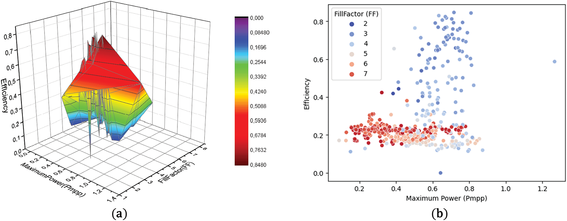
Figure 11: (a) Effect of effect of Fill Factor (FF) and maximum power (Pmpp) on PV panel efficiency with multiple linear regression (b) The effect of effect of Fill Factor (FF) and maximum power (Pmpp) of maximum power on PV panel efficiency with Random Forest
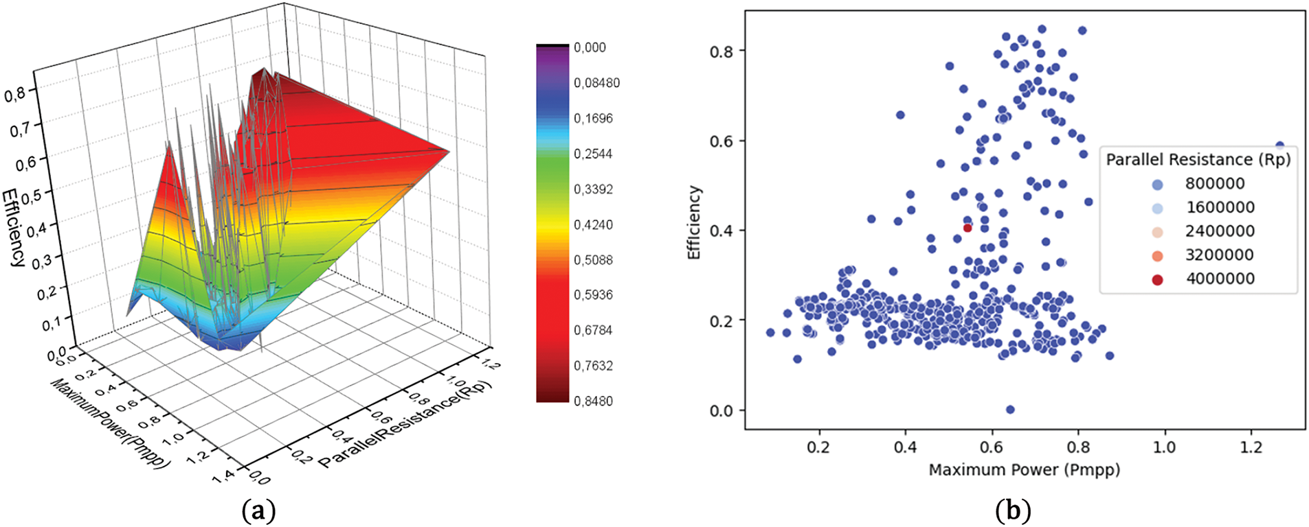
Figure 12: (a) Effect of parallel resistance (Rp) and maximum power (Pmpp) on PV panel efficiency with multiple linear regression (b) The effect of parallel resistance (Rp) and maximum power (Pmpp) of maximum power on PV panel efficiency with Random Forest

Figure 13: (a) Effect of series resistance (Rs) and maximum power (Pmpp) on PV panel efficiency with multiple linear regression (b) The effect of series resistance (Rs) and maximum power (Pmpp) of maximum power on PV panel efficiency with Random Forest
Fig. 10a distinctly illustrates the association among the parameters through its excessive dimensional representation. Fig. 10b illustrates the Random Forest regression plot, which demonstrates a robust positive association between the two variables. The ANOVA result of less than 0.0001 (p < 0.0001) in Fig. 10a signifies a substantial enhancement in panel efficiency. The explanatory power of panel efficiency is around R2 = 0.724. The analysis of the goodness of fit of the values was conducted using linear regression within Random Forest, revealing a strong correlation among the parameters. In Eq. (11), if the highest voltage (Umpp) is below 17.8332, it is multiplied by the positive component of this difference and does not influence efficiency. If the highest voltage (Umpp) exceeds 17.8332, this parameter becomes null and does not influence efficiency.
Eq. (12) demonstrates that Maximum Power (Pmpp) and Fill Factor (FF) exert a consistently augmenting influence. This is seen in Fig. 11a,b. Fig. 11b illustrates that the darker hues are localized at a certain location. A decreased fill factor (FF) correlates with an increased beneficial impact on panel efficiency. As the FF increases, lighter colors ascend and exhibit a diminishing influence. The correlation between the binary parameters (Maximum Power (Pmpp) and Fill Factor (FF)) and Maximum Power (Pmpp) for the panel is about R2 = 0.987, indicating a very high goodness of fit.
Effect of Parallel Resistance (Rp) and Maximum power (Pmpp) on PV panel efficiency.
The impact of Parallel Resistance (Rp) and Maximum Power (Pmpp) on efficiency, as analyzed using linear regression in Random Forest, exhibits a consistently diminishing effect, as illustrated in Fig. 12b. The correlation between panel efficiency and Maximum Power (Pmpp) was determined to be R2 = 0.318, indicating a substantial goodness of fit between the two parameters. In Fig. 12b, the augmentation of parallel resistance diminishes the panel efficiency. The effect of parallel resistance diminishes. The identical scenario is seen in Fig. 11a. Eq. (13) is also observable.
Effect of Series Resistance (Rs) and Maximum power on PV panel efficiency.
The correlation between panel efficiency and Pmax was determined to be R2 = 0.78, indicating a strong goodness of fit between the two parameters. Fig. 13a illustrates that an increase in series resistance correlates with an enhancement in solar panel efficiency. The efficiency of solar panels varies directly with maximum power output. This phenomenon is also illustrated in Fig. 13b, demonstrating the impact of series resistance on this direct proportion. Augmenting the series resistance is directly proportional to both the panel efficiency and the maximum power. This is also seen in Eq. (14).
The elevated R2 values of the subsequent parameters indicate the influence of external factors on the efficiency of PV solar panels, as illustrated in Figs. 14–17.

Figure 14: (a) Effect of air humidity and air humidity on PV panel efficiency with multiple linear regression (b) The effect of air humidity and air humidity of maximum power on PV panel efficiency with Random Forest

Figure 15: (a) Effect of air temperature and air humidity on PV panel efficiency with multiple linear regression (b) The effect of air temperature and air humidity of maximum power on PV panel efficiency with Random Forest

Figure 16: (a) Effect of solar irradiation and air humidity on PV panel efficiency with multiple linear regression (b) The effect of solar irradiation and air humidity of maximum power on PV panel efficiency with Random Forest

Figure 17: (a) Effect of wind direction and air humidity on PV panel efficiency with multiple linear regression (b) The effect of wind direction and air humidity of maximum power on PV panel efficiency with Random Forest
Effect of air humidity and air humidity on PV panel efficiency.
Fig. 14a illustrates a distinctly weak association among the parameters in the spider web depiction. Fig. 14b illustrates a similar weak and negative correlation in the linear regression of the Random Forest plot. The disclosure percentage was approximately R2 = 0.243. If the Air Humidity value exceeds 47.1993, it is multiplied by the positive component of this difference, resulting in a reduction of the efficiency rating (Eq. (15)). If the Air Humidity value exceeds 75.4942, it is multiplied by the positive component of this difference, hence enhancing the efficiency value.
Effect of air temperature and air humidity on PV panel efficiency.
If the air temperature exceeds 21.3839 and the air humidity surpasses 47.1993, the efficiency value is augmented by the product of the positive components of these two discrepancies. In Fig. 15a,b, Eq. (16) indicates that temperature exerts a consistently diminishing influence, but humidity exerts a continually augmenting effect. The goodness of fit between the binary parameters (temperature and air humidity) and panel efficiency is around R2 = 0.712, showing a high level of correlation.
Effect of solar irradiation and air humidity on PV panel efficiency.
In Fig. 16, if air humidity is below 75.4942 and irradiation exceeds 0.2518, it is amplified by the product of the positive components of these two discrepancies, hence diminishing panel efficiency. If air humidity is below 75.4942 and irradiation is below 0.2518, it is increased by the product of the positive components of these two discrepancies, hence enhancing efficiency. The goodness of fit for the parameters is R2 = 0.64624, indicating a strong correlation between them. The augmentation of solar radiation enhances panel efficiency, whereas dampness diminishes it. This is shown in Eq. (17).
Effect of wind direction and air humidity on PV panel efficiency.
If air humidity is below 75.4942, wind direction is below 249.1621, and wind direction spread exceeds 365.0159, multiply by the product of the positive components of these three discrepancies and decrease efficiency. Fig. 17 in Eq. (18) illustrates the consistently diminishing effect of air humidity. Conversely, wind direction exerts a perpetually amplifying influence. The goodness of fit between the binary parameters (temperature and air humidity) and panel efficiency is around R2 = 0.612, showing a high level of correlation. Similar to the impact of solar heat and humidity on panel efficiency, an increase in wind speed, correlated with wind direction and humidity, will diminish the heating of the panel and enhance its efficiency. Elevated humidity exerts a diminishing influence. Lower humidity enhances panel efficiency. This is seen in the figures and the equation.
4.2 Multi-Layer Perceptron’s (MLP) Architecture and Interpretation
We performed tests utilizing the MLP architecture with varying numbers of layers and activation functions. Tables 8 and 9 display the efficiency forecasts based on indoor and outdoor characteristics, respectively. The tables present the results of MAE, MSE, RMSE, and R2 derived from the models. The metrics are determined using the subsequent equations. The MAE (Eq. (19)) measures the mean magnitude of the absolute discrepancies between expected and actual values. The MSE (Eq. (20)) evaluates the mean squared differences between expected and actual values. The RMSE (Eq. (21)), the square root of the MSE, quantifies the model’s prediction accuracy by assessing the square root of the mean squared discrepancies between predicted and observed values. The R2 (Eq. (22)) value indicates the extent to which the variance in the dependent variable is elucidated by the independent factors.


The sigmoid activation function demonstrates optimal performance in the 5-layer model, achieving an MAE of 0.009, MSE of 0.001, RMSE of 0.017, and R2 of 0.990. Typically, an increase in the number of layers correlates with enhanced performance, evidenced by a reduction in MAE and RMSE, alongside an elevation in R2. The tanh and ReLU activation functions exhibit commendable performance, however they somewhat underperform relative to the sigmoid function. The tanh activation function demonstrates optimal performance in the 4-layer and 5-layer models, with MAEs of 0.012 and 0.011, an MSE of 0.001, an RMSE of 0.023, and a R2 of 0.983. The sigmoid activation function exhibits inferior performance with outdoor parameters compared to interior characteristics, achieving optimal results in the 5-layer model. The reel activation function has inferior performance relative to indoor settings, however remains broadly acceptable. Models trained with indoor parameters typically surpass those trained with outdoor parameters. The sigmoid activation function exhibits optimal performance with indoor characteristics, whereas the tanh function excels with outdoor parameters. Performance often enhanced with an increase in the number of layers, indicating that deeper networks produce superior outcomes. Figs. 18 and 19 display the R2 values generated by various models and activation functions for indoor and outdoor parameters, respectively. The 5-layer sigmoid model yields the greatest result in Fig. 18. Fig. 19 clearly indicates that the 4-layer and 5-layer tanh models yield the highest R2 values for the outside parameters.
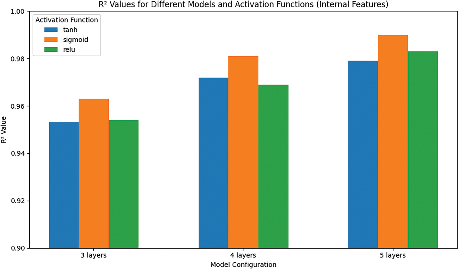
Figure 18: The R2 values for different models and activation functions (indoor features)

Figure 19: The R2 values for different models and activation functions (outdoor features)
Fig. 20 and Table 10 illustrate the impact of both indoor and outdoor parameters on the efficiency estimates of photovoltaic systems. The analysis reveals that the most significant factor influencing efficiency is the Fill Factor. The Fill Factor serves as a critical metric for evaluating the quality of a photovoltaic cell as a power source, representing the ratio of the maximum power to the product of open circuit voltage and short circuit current. The analysis presented in Fig. 20 was conducted using the IBM SPSS software (version 23), a licensed statistical analysis program.

Figure 20: Importance of indoor and outdoor parameters for MLP regression

Solar power plants are a clean and sustainable energy source, playing a crucial role in the future of the energy sector. These resources are essential for meeting growing energy demands, with the potential to generate vast amounts of power. In this context, research aimed at improving solar energy efficiency is of paramount importance. Several factors influence solar energy production, including solar radiation intensity, weather conditions, geographical location, seasonal variations, time of day, surface angle, and cleanliness. These challenges can cause issues in energy production, such as difficulties in storing excess energy and increased costs due to energy shortfalls. By leveraging this data, machine learning algorithms can analyze the impact of weather conditions on solar energy generation and forecast future energy production levels. As a result, integrating solar energy data with meteorological data provides a valuable resource for forecasting solar energy production, enhancing system efficiency, and creating more sustainable energy strategies. A precise analysis of this data, combined with machine learning techniques, can significantly improve the future performance and effectiveness of the solar energy sector.
The study included distinct assessments of indoor and outdoor variables to evaluate their influence on panel efficiency. Essential indoor parameters comprised Open Circuit Voltage (Voc), Short Circuit Current (Isc), Maximum Power (Pmpp), Maximum Voltage (Umpp), Maximum Current (Impp), Fill Factor (FF), Parallel Resistance (Rp), Series Resistance (Rs), and Module Temperature. Key outdoor factors encompassed Air Temperature, Air Humidity, Dew Point, Air Pressure, Irradiation, Irradiation Variability, Wind Speed, Wind Speed Variability, Wind Direction, and Wind Direction Variability. The inclusion of these factors as input data enhanced the performance of the MLP model, especially for short-term predictions. Among the interior parameters, Fill Factor (FF), Series Resistance (Rs), Parallel Resistance (Rp), Maximum Voltage (Umpp), and Module Temperature were recognized as significantly influencing the energy efficiency of the photovoltaic panels. Likewise, sun irradiance, air humidity, module power, wind speed direction, and the dispersion of wind speed direction were among the most significant external variables. By understanding the effect of these measures, stakeholders can analyze the PV panel design to improve the energy output. The main aim of this work was to assess the efficiency of photovoltaic systems and to clarify the elements affecting these estimations through several machine learning algorithms. Future research should validate the models’ performance using datasets from diverse climates and geographical regions to confirm their applicability beyond the Utrecht University setting. The integration of new data and better efficiency processes are key future areas of work for this study.
This study’s data is also limited to the specific conditions of Utrecht University and has a temperate maritime climate, it is likely that models trained from this data will not be as effective in other areas. For future modeling efforts, we hope to leverage the methods used by the ‘Dendrite neural network scheme for estimating output power and efficiency for a class of solar free-piston Stirling engine generator’ [55] to create a model that is effective despite locational differences and that can also utilize data from numerous locations.
This study examined the indoor and exterior variables and influencing factors affecting the energy output of photovoltaic (PV) solar panels installed on the roof of the Faculty of Science at Utrecht University. We utilized the Multi-Layer Perceptrons (MLP) model, Multivariate Adaptive Regression Splines (MARS) model, Multiple Linear Regression (MLR) model, and the Random Forest (RF) model to assess the energy efficiency of these photovoltaic systems. Future studies should compare these models with others, using models from PVsyst, PVlib, or other reputable sources as benchmarks. Notwithstanding the data irregularities, the MLP model exhibited enhanced performance throughout the evaluations. Artificial neural networks, especially the MLP model, have garnered significant attention in recent years, owing to their strong capacity to describe nonlinear interactions. This research employed both MLP and RF models to forecast the efficiency of the solar power system. The regression analyses demonstrated robust predictive ability, with R2 values around 1, underscoring the models’ efficacy. The performance measures, comprising R2, RMSE, MAE, and MAPE, substantiated the effectiveness of the MLP model, which attained a R2 value of 0.983 for both indoor and outdoor parameters. In contrast, the RF model attained a R2 value of 0.956 for outdoor parameters and 0.975 for inside parameters. The MLP model surpassed the RF model, attaining a Mean Absolute Error (MAE) of 0.012 for outdoor parameters and 0.09 for indoor values, as well as a Root Mean Square Error (RMSE) of 0.023 for outdoor parameters and 0.017 for indoor parameters. These findings corroborate prior research, highlighting the efficacy of the MLP model in assessing solar panel efficiency. This paper underlines the underutilization of the MLP model in photovoltaic solar power plant efficiency research and highlights its potential contributions to the energy forecasting literature.
Acknowledgement: Not applicable.
Funding Statement: The authors received no specific funding for this study.
Author Contributions: Methodology, Ihsan Levent, Gökhan Şahin, Gültekin Işık, Wilfried van Sark and Sabir Rustemli; Software, Gökhan Şahin and Wilfried van Sark; Formal analysis, Methodology, Ihsan Levent, Gökhan Şahin, Gültekin Işık, Wilfried van Sark and Sabir Rustemli; Investigation, Methodology, Ihsan Levent, Gökhan Şahin, Gültekin Işık, Wilfried van Sark and Sabir Rustemli; Writing original draft, Methodology, Ihsan Levent, Gökhan Şahin, Gültekin Işık, Wilfried van Sark and Sabir Rustemli; Writing—review & editing, Methodology, Ihsan Levent, Gökhan Şahin, Gültekin Işık, Wilfried van Sark and Sabir Rustemli. All authors reviewed the results and approved the final version of the manuscript.
Availability of Data and Materials: The datasets generated and/or analyzed during the current study are available from the corresponding author upon reasonable request.
Ethics Approval: Not applicable.
Conflicts of Interest: The authors declare no conflicts of interest to report regarding the present study.
Nomenclature
| PV | Photovoltaic |
| MLP | Multi-Layer Perceptron |
| MARS | Multivariate Adaptive Regression Spline |
| MLR | Multiple Linear Regression |
| RF | Random Forest |
| Voc | Open Circuit Voltage |
| Isc | Short Circuit Current |
| Pmpp | Maximum Power |
| Umpp | Maximum Voltage |
| Impp | Maximum Current |
| FF | Fill Factor |
| Rp | Parallel Resistance |
| Rs | Series Resistance |
| MAE | Mean Absolute Error |
| MSE | Mean Squared Error |
| RMSE | Root Mean Squared Error |
References
1. Şenkal O, Kuleli T. Estimation of solar radiation over Turkey using artificial neural network and satellite data. Appl Energy. 2009;86(7–8):1222–8. doi:10.1016/j.apenergy.2008.06.003. [Google Scholar] [CrossRef]
2. Badescu V. Modeling solar radiation at the earth’s surface. Berlin/Heidelberg, Germany: Springer; 2014. p.517. [Google Scholar]
3. Mellit A. Artificial intelligence technique for modelling and forecasting of solar radiation data: a review. Int J Artif Intell Soft Comput. 2008;1(1):52. doi:10.1504/IJAISC.2008.021264. [Google Scholar] [CrossRef]
4. Besharat F, Dehghan AA, Faghih AR. Empirical models for estimating global solar radiation: a review and case study. Renew Sustain Energy Rev. 2013;21(4):798–821. doi:10.1016/j.rser.2012.12.043. [Google Scholar] [CrossRef]
5. Fan J, Wang X, Wu L, Zhou H, Zhang F, Yu X, et al. Comparison of support vector machine and extreme gradient boosting for predicting daily global solar radiation using temperature and precipitation in humid subtropical climates: a case study in china. Energy Convers Manag. 2018;164(8):102–11. doi:10.1016/j.enconman.2018.02.087. [Google Scholar] [CrossRef]
6. Guermoui M, Abdelaziz R, Gairaa K, Djemoui L, Benkaciali S. New temperature-based predicting model for global solar radiation using support vector regression. Int J Ambient Energy. 2022;43(1):1397–407. doi:10.1080/01430750.2019.1708792. [Google Scholar] [CrossRef]
7. Mohsenzadeh Karimi S, Kisi O, Porrajabali M, Rouhani-Nia F, Shiri J. Evaluation of the support vector machine, random forest and geo-statistical methodologies for predicting long-term air temperature. ISH J Hydraul Eng. 2020;26(4):376–86. doi:10.1080/09715010.2018.1495583. [Google Scholar] [CrossRef]
8. Shiri J, Kişi Ö, Landeras G, López JJ, Nazemi AH, Stuyt LCPM. Daily reference evapotranspiration modeling by using genetic programming approach in the Basque Country (Northern Spain). J Hydrol. 2012;414(2):302–16. doi:10.1016/j.jhydrol.2011.11.004. [Google Scholar] [CrossRef]
9. Landeras G, López JJ, Kisi O, Shiri J. Comparison of gene expression programming with neuro-fuzzy and neural network computing techniques in estimating daily incoming solar radiation in the Basque Country (Northern Spain). Energy Convers Manag. 2012;62(1):1–13. doi:10.1016/j.enconman.2012.03.025. [Google Scholar] [CrossRef]
10. Güçlü YS, Yeleğen MÖ, Dabanlı İ, Şişman E. Solar irradiation estimations and comparisons by ANFIS, Angström-Prescott and dependency models. Sol Energy. 2014;109(3):118–24. doi:10.1016/j.solener.2014.08.027. [Google Scholar] [CrossRef]
11. Kozak M, ve Kozak Ş. Enerji depolama yöntemleri. Uluslararası Teknol Bilim Derg. 2012;4(2):17–29. [Google Scholar]
12. Saad B, El Hannani A, Errattahi R, Aqqal A. Assessing the impact of weather forecast models combination on the AMS solar energy prediction. In: 2020 Fourth International Conference on Intelligent Computing in Data Sciences (ICDS); 2020 Oct 21–23; Fez, Morocco. p. 1–5. doi:10.1109/icds50568.2020.9268767. [Google Scholar] [CrossRef]
13. Alizamir M, Kim S, Kisi O, Zounemat-Kermani M. A comparative study of several machine learning based non-linear regression methods in estimating solar radiation: case studies of the USA and Turkey regions. Energy. 2020;197(1):117239. doi:10.1016/j.energy.2020.117239. [Google Scholar] [CrossRef]
14. Shahid F, Zameer A, Afzal M, Hassan M. Short term solar energy prediction by machine learning algorithms; arXiv:2012.00688. 2020. [Google Scholar]
15. Araf I, Elkhadiri H, Errattahi R, El Hannani A. AMS solar energy prediction: a comparative study of regression models. In: 2019 Third International Conference on Intelligent Computing in Data Sciences (ICDS); 2019 Oct 28–30; Marrakech, Morocco. p. 1–5. doi:10.1109/icds47004.2019.8942237. [Google Scholar] [CrossRef]
16. Díaz-Vico D, Torres-Barrán A, Omari A, Dorronsoro JR. Deep neural networks for wind and solar energy prediction. Neural Process Lett. 2017;46(3):829–44. doi:10.1007/s11063-017-9613-7. [Google Scholar] [CrossRef]
17. Aggarwal SK, Saini LM. Solar energy prediction using linear and non-linear regularization models: a study on AMS (American Meteorological Society) 2013–14 Solar Energy Prediction Contest. Energy. 2014;78(2):247–56. doi:10.1016/j.energy.2014.10.012. [Google Scholar] [CrossRef]
18. Bakhashwain JM. Prediction of global solar radiation using support vector machines. Int J Green Energy. 2016;13(14):1467–72. doi:10.1080/15435075.2014.896256. [Google Scholar] [CrossRef]
19. Torres-Barrán A, Alonso Á, Dorronsoro JR. Regression tree ensembles for wind energy and solar radiation prediction. Neurocomputing. 2019;326(7):151–60. doi:10.1016/j.neucom.2017.05.104. [Google Scholar] [CrossRef]
20. Belaid S, Mellit A. Prediction of daily and mean monthly global solar radiation using support vector machine in an arid climate. Energy Convers Manag. 2016;118:105–18. doi:10.1016/j.enconman.2016.03.082. [Google Scholar] [CrossRef]
21. Hassan GE, Youssef ME, Mohamed ZE, Ali MA, Hanafy AA. New temperature-based models for predicting global solar radiation. Appl Energy. 2016;179:437–50. doi:10.1016/j.apenergy.2016.07.006. [Google Scholar] [CrossRef]
22. Laidi M, Hanini S, Rezrazi A, Yaiche MR, El Hadj AA, Chellali F. Supervised artificial neural network-based method for conversion of solar radiation data (case study: algeria). Theor Appl Climatol. 2017;128(1):439–51. doi:10.1007/s00704-015-1720-7. [Google Scholar] [CrossRef]
23. Chiteka K, Enweremadu C. Prediction of global horizontal solar irradiance in Zimbabwe using artificial neural networks. J Clean Prod. 2016;135(4):701–11. doi:10.1016/j.jclepro.2016.06.128. [Google Scholar] [CrossRef]
24. Wang L, Kisi O, Zounemat-Kermani M, Zhu Z, Gong W, Niu Z, et al. Prediction of solar radiation in China using different adaptive neuro-fuzzy methods and M5 model tree. Int J Climatol. 2017;37(3):1141–55. doi:10.1002/joc.4762. [Google Scholar] [CrossRef]
25. Hassan MA, Khalil A, Kaseb S, Kassem MA. Exploring the potential of tree-based ensemble methods in solar radiation modeling. Appl Energy. 2017;203:897–916. doi:10.1016/j.apenergy.2017.06.104. [Google Scholar] [CrossRef]
26. Basaran K, Özçift A, Kılınç D. A new approach for prediction of solar radiation with using ensemble learning algorithm. Arab J Sci Eng. 2019;44(8):7159–71. doi:10.1007/s13369-019-03841-7. [Google Scholar] [CrossRef]
27. Gülşen K, Sönmez ME, Karabaş M. Gaziantep İlinde güneş enerjisi potansiyelinin Analitik Hiyerarşi Süreci Yöntemi (AHP) İle belirlenmesi. Coğrafya Derg. 2019;39:61–72. doi:10.26650/JGEOG2019-0031. [Google Scholar] [CrossRef]
28. Ibrahim S, Daut I, Irwan YM, Irwanto M, Gomesh N, Farhana Z. Linear regression model in estimating solar radiation in Perlis. Energy Proc. 2012;18:1402–12. doi:10.1016/j.egypro.2012.05.156. [Google Scholar] [CrossRef]
29. Kisi O. Pan evaporation modeling using least square support vector machine, multivariate adaptive regression splines and M5 model tree. J Hydrol. 2015;528(12):312–20. doi:10.1016/j.jhydrol.2015.06.052. [Google Scholar] [CrossRef]
30. Li DHW, Chen W, Li S, Lou S. Estimation of hourly global solar radiation using Multivariate Adaptive Regression Spline (MARS)—a case study of Hong Kong. Energy. 2019;186(1):115857. doi:10.1016/j.energy.2019.115857. [Google Scholar] [CrossRef]
31. Işık G, Ekici S, Şahin G. A neural network model for UAV propulsion system. Aircr Eng Aerosp Technol. 2020;92(8):1177–84. doi:10.1108/AEAT-04-2020-0064. [Google Scholar] [CrossRef]
32. AlShafeey M, Csáki C. Evaluating neural network and linear regression photovoltaic power forecasting models based on different input methods. Energy Rep. 2021;7:7601–14. doi:10.1016/j.egyr.2021.10.125. [Google Scholar] [CrossRef]
33. Kim YS, Joo HY, Kim JW, Jeong SY, Moon JH. Use of a big data analysis in regression of solar power generation on meteorological variables for a Korean solar power plant. Appl Sci. 2021;11(4):1776. doi:10.3390/app11041776. [Google Scholar] [CrossRef]
34. Ritonga NA. Estimation of multivariate adaptive regression splines (MARS) model parameters by using generalized least square (GLS) method. JMEA J Math Educ Appl. 2023;2(2):62–72. doi:10.30596/jmea.v2i2.13106. [Google Scholar] [CrossRef]
35. El-Aal SA, Alqabli MA, Naim AA. Forecasting solar photovoltaic energy production using linear regression-based techniques. J Theor Appl Inf Technol. 2023;101(9):3326–37. [Google Scholar]
36. Nedaei A, Eskandari A, Milimonfared J, Aghaei M. Fault resistance estimation for line-line fault in photovoltaic arrays using regression-based dense neural network. Eng Appl Artif Intell. 2024;133:108067. doi:10.1016/j.engappai.2024.108067. [Google Scholar] [CrossRef]
37. Paluang P, Thavorntam W, Phairuang W. Application of multilayer perceptron artificial neural network (MLP-ANN) algorithm for PM2.5 mass concentration estimation during open biomass burning episodes in Thailand. Int J Geoinform. 2024;20(7):28–42. doi:10.52939/ijg.v20i7.3401. [Google Scholar] [CrossRef]
38. Şahin G, van Sark WGJHM. Machine learning-based evaluation of solar photovoltaic panel exergy and efficiency under real climate conditions. Energies. 2025;18(6):1318. doi:10.3390/en18061318. [Google Scholar] [CrossRef]
39. Agarap AF. Deep learning using rectified linear units (ReLU). arXiv:1803.08375. 2018. [Google Scholar]
40. He K, Zhang X, Ren S, Sun J. Delving deep into rectifiers: surpassing human-level performance on ImageNet classification. In: Proceedings of the IEEE International Conference on Computer Vision (ICCV); 2015 Dec 7–13; Santiago, Chile. p. 1026–34. doi:10.1109/ICCV.2015.123. [Google Scholar] [CrossRef]
41. Kingma DP, Ba J, Hammad MM. Adam: a method for stochastic optimization. arXiv:1412.6980. 2014. [Google Scholar]
42. Goodfellow I, Bengio Y, Courville A. Deep learning. Cambridge, MA, USA: MIT Press; 2016. [Google Scholar]
43. Sahin G, Isik G, van Sark WGJHM. Predictive modeling of PV solar power plant efficiency considering weather conditions: a comparative analysis of artificial neural networks and multiple linear regression. Energy Rep. 2023;10(10):2837–49. doi:10.1016/j.egyr.2023.09.097. [Google Scholar] [CrossRef]
44. Alkan O, Genc A, Oktay E, Celik AK. Electricity consumption analysis using spline regression models: the case of a Turkish Province. Asian Soc Sci. 2013;9(7):231–40. doi:10.5539/ass.v9n7p231. [Google Scholar] [CrossRef]
45. Eyduran E, ve Duman H. R yazılımı ile multivariate adaptive regression splines (MARS) uygulaması ders notları (Multivariate adaptive regression spline (MARS) Application with R software lecture notes). [cited 2025 Jan 1]. Available from: https://www.researchgate.net/publication/340077587_R_yazilimi_ile_multivariate_adaptive_regression_splines_mars_uygulamasi_ders_notlari. [Google Scholar]
46. Friedman JH. Multivariate adaptive regression splines. Ann Statist. 1991;19(1):1–67. doi:10.1214/aos/1176347963. [Google Scholar] [CrossRef]
47. Ali Sahraei M, Duman H, Çodur MY, Eyduran E. Prediction of transportation energy demand: multivariate adaptive regression splines. Energy. 2021;224(4):120090. doi:10.1016/j.energy.2021.120090. [Google Scholar] [CrossRef]
48. Kornacki J, Ćwik J. Statistical learning systems. Warsaw, Poland: WNT Warsaw; 2005. (In Polish). [Google Scholar]
49. Sahin G, Eyduran E, Turkoglu M, Sahin F. Estimation of global irradiation parameters at location of migratory birds in Iğdir, Turkey by means of MARS algorithm. Pak J Zool. 2018;50(6):2317–24. doi:10.17582/journal.pjz/2018.50.6.2317.2324. [Google Scholar] [CrossRef]
50. Duzen H, Aydin H. Sunshine-based estimation of global solar radiation on horizontal surface at Lake Van region (Turkey). Energy Convers Manag. 2012;58(4):35–46. doi:10.1016/j.enconman.2011.11.028. [Google Scholar] [CrossRef]
51. Eyduran E, Yakubu A, Duman H, Aliyev P, Tırınk C. Predictive modeling of multivariate adaptive regression splines: an R tutorial. In: Çelik Ş, editor. Veri Madenciliği Yöntemleri: Tarim Alanında Uygulamaları. Şişli, Istanbul: Rating Academy; 2020. p. 25–48. [Google Scholar]
52. Chen YJ, Lin JA, Chen YM, Wu JH. Financial forecasting with multivariate adaptive regression splines and queen genetic algorithm-support vector regression. IEEE Access. 2019;7:112931–8. doi:10.1109/ACCESS.2019.2927277. [Google Scholar] [CrossRef]
53. Put R, Xu QS, Massart DL, Vander Heyden Y. Multivariate adaptive regression splines (MARS) in chromatographic quantitative structure—retention relationship studies. J Chromatogr A. 2004;1055(1–2):11–9. doi:10.1016/j.chroma.2004.07.112. [Google Scholar] [CrossRef]
54. Droogers P, Allen R. Estimating reference evapotranspiration under inaccurate data conditions. Irrig Drain Syst. 2002;16(1):33–45. doi:10.1023/A:1015508322413. [Google Scholar] [CrossRef]
55. Shourangiz-Haghighi A, Tavakolpour-Saleh AR. A neural network-based scheme for predicting critical unmeasurable parameters of a free piston Stirling oscillator. Energy Convers Manag. 2019;196(10):623–39. doi:10.1016/j.enconman.2019.06.035. [Google Scholar] [CrossRef]
56. Maulud D, Abdulazeez AM. A review on linear regression comprehensive in machine learning. J Appl Sci Technol Trends. 2020;1(2):140–7. doi:10.38094/jastt1457. [Google Scholar] [CrossRef]
57. Breiman L. Random forest. Mach Learn. 2001;45(1):5–32. doi:10.1023/A:1010933404324. [Google Scholar] [CrossRef]
58. Ali J, Khan R, Ahmad N, Maqsood I. Random forests and decision trees. Int J Comput Sci Issues. 2012;9(5):272–8. [Google Scholar]
59. Schonlau M, Zou RY. The random forest algorithm for statistical learning. Stata J Promot Commun Stat Stata. 2020;20(1):3–29. doi:10.1177/1536867X20909688. [Google Scholar] [CrossRef]
Cite This Article
 Copyright © 2025 The Author(s). Published by Tech Science Press.
This work is licensed under a Creative Commons Attribution 4.0 International License , which permits unrestricted use, distribution, and reproduction in any medium, provided the original work is properly cited.
 Downloads
 Citation Tools