Multi-Neighborhood Enhanced Harris Hawks Optimization for Efficient Allocation of Hybrid Renewable Energy System with Cost and Emission Reduction

1  Introduction

1.1 Background and Motivation

The global energy landscape is undergoing a significant transformation, driven by the imperative of sustainable development and climate change mitigation [1]. The surge in adopting sustainable and renewable energy sources (RES) worldwide can be attributed to various factors, including population growth, industrial development, and energy stability [2,3]. This demand is especially pronounced in major electricity-consuming countries such as China, the USA, India, Russia, and Japan [2]. The transition to renewable energy is viewed as a critical solution to environmental challenges and a means to reduce dependency on fossil fuels [3].

This transition drove the development of Hybrid Renewable Energy Systems (HRES), which integrate multiple renewable energy technologies, such as solar, wind, hydropower, and geothermal, to create a more reliable and efficient power supply. HRES offers numerous advantages: cost-effectiveness, scalability, reduced environmental impact, and consistent power supply through the complementary nature of different energy sources. These systems are particularly beneficial in optimizing energy production, as they utilize data-driven frameworks incorporating machine learning and hybrid metaheuristics to predict weather patterns and system performance over their lifespan, ensuring realistic capacity planning and improved reliability in changing weather conditions [4].

In a comprehensive meta-analysis, Ref. [5] analyzed 348 papers published between 2017 and 2022, identifying four critical applications within HRES: predicting renewable energy generation, coordinating and virtually aggregating energy resources, implementing demand response strategies, and optimizing grid management. For instance, in the domain of energy prediction, the study reported an impressive reduction in error ratio to as low as 3%. This extensive research highlights the significant advancements and contributions made by researchers toward enhancing the efficiency and effectiveness of HRES, demonstrating a substantial impact in this field.

Another comprehensive review by [6] outlines three primary components of HRES: fuel consumption, energy storage, and renewable energy sources. Fuel consumption encompasses diesel and gas generators. Energy storage includes technologies such as hydrogen storage, pumped hydro storage, compressed air energy storage, thermal storage, flywheel energy storage, and ultra/supercapacitors. Renewable energy sources are solar photovoltaic, wind turbine, hydropower, biogas generator, and tidal power.

The review identifies three primary objective functions for HRES optimization: economic, reliability, and technical/emission objectives. Economic objectives include net present cost (NPC), levelized cost of energy (LCOE), total annual cost (TAC), simple payback period (SPP), cost of energy (COE), internal rate of return (IRR), and cost of interruption energy. Reliability objectives consist of loss of power supply probability (LPSP), expected energy not supplied (EENS), loss of load expectation (LOLE), loss of energy expectation (LOEE), system average interruption frequency index (SAIFI), system average interruption duration index (SAIDI), and energy index ratio. Technical and emission objectives cover demand energy, renewable factors (RF), carbon emission (CE), customer comfort level (CCL), battery longevity (BL), and discharged energy (DE).

Constraints are classified into technical constraints and component-associated constraints. Technical constraints include power balance, frequency fluctuation, power reserve, and voltage fluctuation. Component-associated constraints involve land accessibility, heights of wind turbine hubs, and the number of components. According to their findings, key optimization objectives for HRES include the cost of energy, total net present cost, life cycle cost, probability of loss of power supply, and discharged energy.

Ref. [6] also identified that the metaheuristic algorithms commonly applied in HRES optimization are predominantly evolutionary algorithms. These include particle swarm optimization (PSO), grey wolf optimization (GWO), whale optimization algorithm (WOA), firefly algorithm (FA), and artificial bee swarm optimization (ABSO). Furthermore, Ref. [7] highlighted the application of various metaheuristics for addressing the size and placement of distributed generation problems, including genetic algorithm (GA), particle swarm optimization (PSO), genetic algorithm-tabu search (GA-TS), improved gravitational search algorithm (IGSA), backtracking search algorithm (BSA), bacterial foraging optimization (BFO), and grey wolf optimization (GWO). These studies underscore the versatility and effectiveness of evolutionary algorithms in optimizing the allocation and performance of HRES, thereby contributing to the reduction of costs and emissions.

While HRES applications span diverse contexts, such as natural reserves [8] and residential power [9], this study focuses specifically on institutional applications. This scope selection is motivated by several factors. First, multiple studies have established performance benchmarks for institutional HRES optimization, particularly for hospitals [10], factories [11], hotels [12], and universities [12]. These institutions share common operational patterns and reliability requirements, enabling meaningful comparative analysis. Second, their similar technical constraints allow for systematic validation of optimization approaches. Third, the mathematical models and algorithms developed for these institutions can serve as a foundation for extending to other HRES applications, while insights gained from institutional optimization can inform broader HRES implementations.

Our motivation stems from the need to address significant research gaps in the allocation of HRES. By optimizing HRES with a focus on critical factors such as battery quantity, charge-discharge efficiency, reliability, and renewable energy fraction, we aim to develop economically competitive, reliable, and environmentally sustainable systems. This study seeks to minimize the levelized cost of energy and pollutant emissions through comprehensive and practical considerations. By applying the optimized HRES to a range of settings, including factories, hotels, universities, and hospitals, this research will demonstrate the scalability and versatility of these systems, ultimately contributing to more sustainable and cost-effective energy solutions.

1.2 Literature Review

Within the four applications in hybrid renewable energy systems classified by Pop et al. [5], optimizing the size and placement of distributed grids is critical for enhancing efficiency and reducing both costs and environmental impacts. Most research in this area has employed population-based metaheuristic algorithms to optimize energy generation, consumption, and battery storage. The primary challenge lies in optimally allocating energy resources to simultaneously serve multiple application tasks, comply with regulatory constraints, and achieve minimal cost and environmental impact. This challenge is further compounded by the need to accurately determine the optimal size and location of distributed generations, as highlighted by Nassef et al. [7]. Their review identifies the necessity of addressing size and placement problems and classifies these challenges based on location dependency and distribution network-related factors.

For the sizing problem of HRES, Agajie et al. [6] summarized the objective functions, constraints, decision variables, and algorithms commonly used in the literature. They reported that various metrics have been utilized for objective functions, including cost of energy (COE), loss of power supply probability (LPSP), life cycle cost (LCC), net present cost (NPC), levelized cost of energy (LCOE), discharged energy (DE), and the number of hours per year that the energy demand exceeds the capacity of the HRES generation system (LOLP). Regarding constraints, typical considerations include the energy of the battery, the number of components, load dissatisfaction rate, loss of power supply probability (LPSP), state of charge (SOC), and load interruption probability. These constraints ensure that the system operates efficiently and reliably under various conditions.

Based on these foundational metrics, recent literature has highlighted the importance of comprehensive sustainability metrics in evaluating HRES performance [13,14]. These metrics span multiple dimensions including technical performance, economic viability, and environmental impact. Technical metrics typically include system reliability measures like Loss of Power Supply Probability (LPSP), energy efficiency indicators such as charge-discharge performance, and capacity utilization metrics. Economic metrics commonly focus on the Levelized Cost of Energy (LCOE) and total operational costs, which incorporate both initial investments and ongoing maintenance expenses [15,16].

Environmental metrics for HRES evaluation can be particularly complex, ranging from immediate operational impacts to long-term sustainability indicators. Key operational metrics include CO2, SO2, and NOx emissions from both storage systems and non-renewable sources, as well as the renewable energy fraction that measures a system’s contribution to clean energy transition (Li et al., 2021). While broader environmental metrics such as life-cycle assessment and exergy efficiency provide valuable insights into system sustainability [14], operational metrics often prove more practical for facility managers due to their accessibility and actionability [12,17].

This study focuses on operational metrics that facility managers can actively monitor and control while acknowledging the importance of broader sustainability indicators. Our selection of metrics emphasizes practical applicability and data availability, supported by their validation in previous research (Elattar & ElSayed, 2020; Kharrich et al., 2020).

Several advanced algorithms have been applied to solve the HRES allocation problem, such as the firefly-inspired algorithm, water cycle algorithm, artificial bee swarm optimization, mutation adaptive differential evolution, and the grey wolf algorithm. These algorithms have been employed to optimize the deployment and performance of HRES, addressing the complexities and challenges associated with the system’s design and operation.

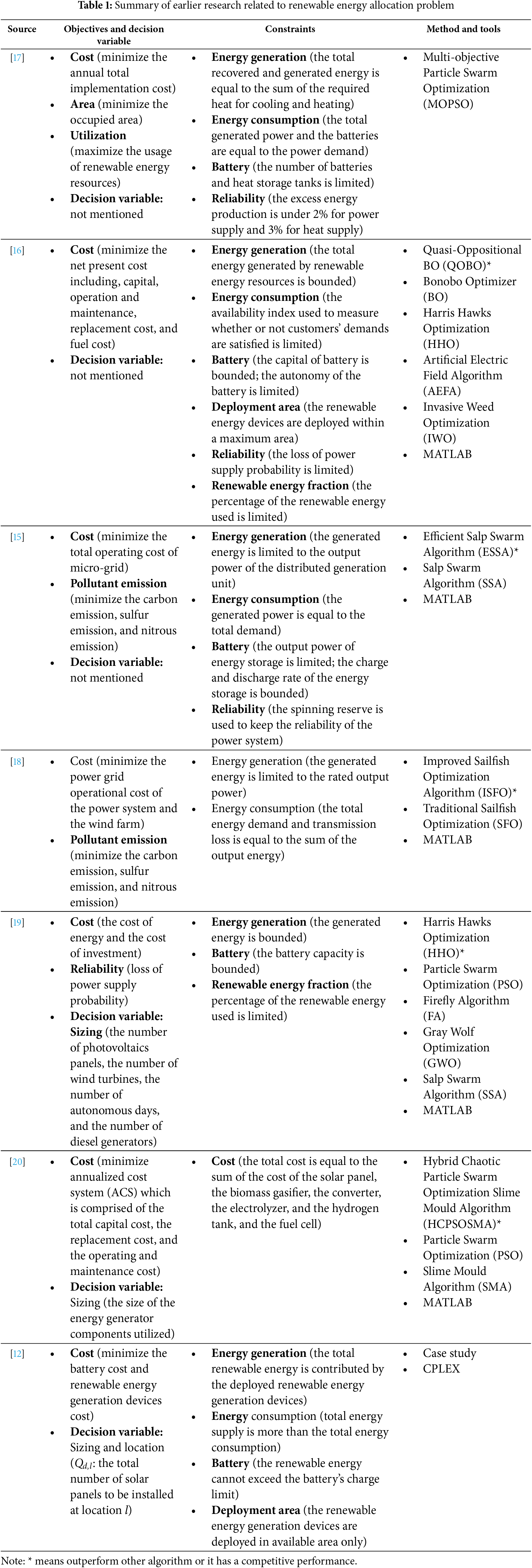
To discuss the optimal allocation problem more deeply, we summarize the related research in Table 1, organized by year. For comparison, we include the source, objective function, constraints, method, and location. From Table 1, it can be observed that the preferred objective functions primarily focus on costs from various perspectives, including implementation cost, net present cost, total operation cost, cost of energy, investment cost, annualized cost of the system, battery cost, and the cost of renewable energy generation devices. Earlier research primarily focused on area utilization, whereas later studies have increasingly emphasized pollutant emissions. Regarding constraints, factors such as energy generation, energy consumption, and battery capacity are widely considered. Although reliability is discussed and defined differently across studies, the loss of power supply probability (LPSP) is a commonly used metric. In terms of methods, MATLAB and CPLEX are used to obtain optimal solutions, while evolutionary algorithms are tailored for approximate solutions.

1.3 Contributions

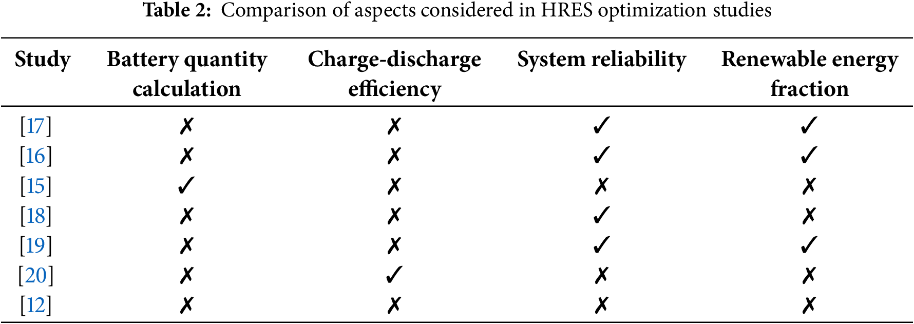
Based on our extensive literature review (summarized in Table 2), we identify specific and critical gaps in achieving optimal allocation of Hybrid Renewable Energy Systems (HRES). These gaps, which have not been collectively addressed in previous research, hinder the development of HRES allocations that can effectively meet modern society’s energy demands while simultaneously optimizing both levelized energy costs and environmental impact.

•   Battery Quantity Calculation: Previous studies have not adequately addressed the impact of the number of batteries on system performance. We reference the battery quantity calculation method organized by [21] to ensure that the system can effectively meet energy demands. For instance, while Kharrich et al. [16] and Çetinbaş et al. [19] consider battery storage in their models, they do not explicitly optimize battery quantities or consider their impact on system performance.

•   Charge-Discharge Efficiency: Studies like Li et al. [18] and Çetinbaş et al. [19] focus on system optimization without accounting for the crucial impact of charge-discharge efficiency on long-term performance and cost. We provide a more realistic representation of battery performance and lifecycle by adopting the charge-discharge efficiency calculation formulas used by [22,23].

•   System Reliability: Reliability is a crucial aspect of energy systems that is often overlooked. While works like Elattar et al. [15] address reliability, they do not integrate it with other critical operational constraints such as battery efficiency and renewable energy fraction. We enhance system reliability using the Loss of Power Supply Probability (LPSP) metric, which ensures that the system can consistently meet energy demands without failure.

•   Renewable Energy Fraction: The proportion of energy derived from renewable sources is essential for assessing the sustainability of HRES. We incorporate the renewable energy fraction calculation method from [24] to evaluate and optimize the renewable contribution to the overall energy mix.

Second, we enhance the algorithmic approach to HRES optimization. Recent studies [2,19] have demonstrated the superiority of Harris Hawks Optimization (HHO) over other metaheuristics for HRES problems. Building on this foundation, we propose an innovative solution that incorporates multiple neighborhood structures specifically designed for HRES optimization. Our enhanced algorithm includes:

•   Introduces three specialized neighborhood structures (SwapDevice, ReduceDevice, and CloseOpenDevice) that effectively navigate the complex solution space of HRES allocation

•   Demonstrates significant improvements over existing methods across different scenarios. Our experimental results show a 46% cost reduction in factory environments, 40% improvement in hospitals, 36% enhancement in hotels, and 39% better performance in universities—each addressing distinct operational demands and reliability requirements

•   Maintains computational efficiency while handling multiple operational constraints

Third, we provide comprehensive validation through extensive testing across four distinct institutional settings with varying reliability requirements:

•   Hospitals with high reliability needs (LPSP = 0.1)

•   Factories with moderate reliability requirements (LPSP = 0.3)

•   Hotels with balanced operational needs (LPSP = 0.3)

•   Universities with flexible reliability constraints (LPSP = 0.6)

Each scenario presents unique challenges and operational requirements, as evidenced by our experimental results. For example, hospitals require consistent power supply with minimal interruptions (LPSP = 0.1), while universities can accommodate more flexible reliability constraints (LPSP = 0.6). This comprehensive validation across diverse operational contexts addresses limitations in previous studies such as [17] and [20], which typically focused on single-scenario applications. Together with our theoretical contributions, this practical validation advances both the fundamental understanding and real-world implementation of HRES optimization, providing a more comprehensive approach to sustainable energy system design.

This paper is organized into five sections, beginning with the introduction. In Section 2, we define the optimization problem under study, detailing the mathematical programming approach, notations, and assumptions. Section 3 introduces the tailored Harris Hawks Optimization (HHO) algorithm. Section 4 outlines the experimental settings, design, and results analysis. Finally, Section 5 presents the overall conclusions of this study.

2  Problem Statement

In this section, we first introduce the notations for the proposed problem. Subsequently, we formally define it using mathematical models and elaborate on the assumptions.

2.1 Notations

Consider an institution planning to deploy n renewable energy devices, intending to deploy them across m available locations to satisfy power demands over a period defined by k. Let N = {1, 2, … , n} be a set of renewable energy devices, M = {1, 2, … , m} be the available locations and T = {1, 2, … , t} be the planning period. We denote by xij the number of device i that are deployed at location j, i ∈N, j ∈ M. Let PDk denote the expected energy demand at each period interval k, which need to be met, k ∈ T. To address these demands, energy generation is collaboratively achieved by renewable energy devices, represented by as Pik, and non-renewable energy source, denoted by P¯k. Any surplus energy generated during this period k is stored in the battery system, represented as EBk.

Furthermore, each renewable energy device requires a specific amount of space, allowing for the allocation of multiple renewable energy devices within each available area Aj. The area Aj is defined as the set of locations where each can accommodate one or more devices, dependent on their spatial requirements, and the space required for each device i is specified by Si. Additionally, each device i incurs different levelized cost of energy, noted as LCOEi. Pollutant emissions from non-renewable energy sources and battery storage systems are tracked and denoted by DEMk and BEMk, respectively. The notations that are used throughout this study are summarized in Table 3.

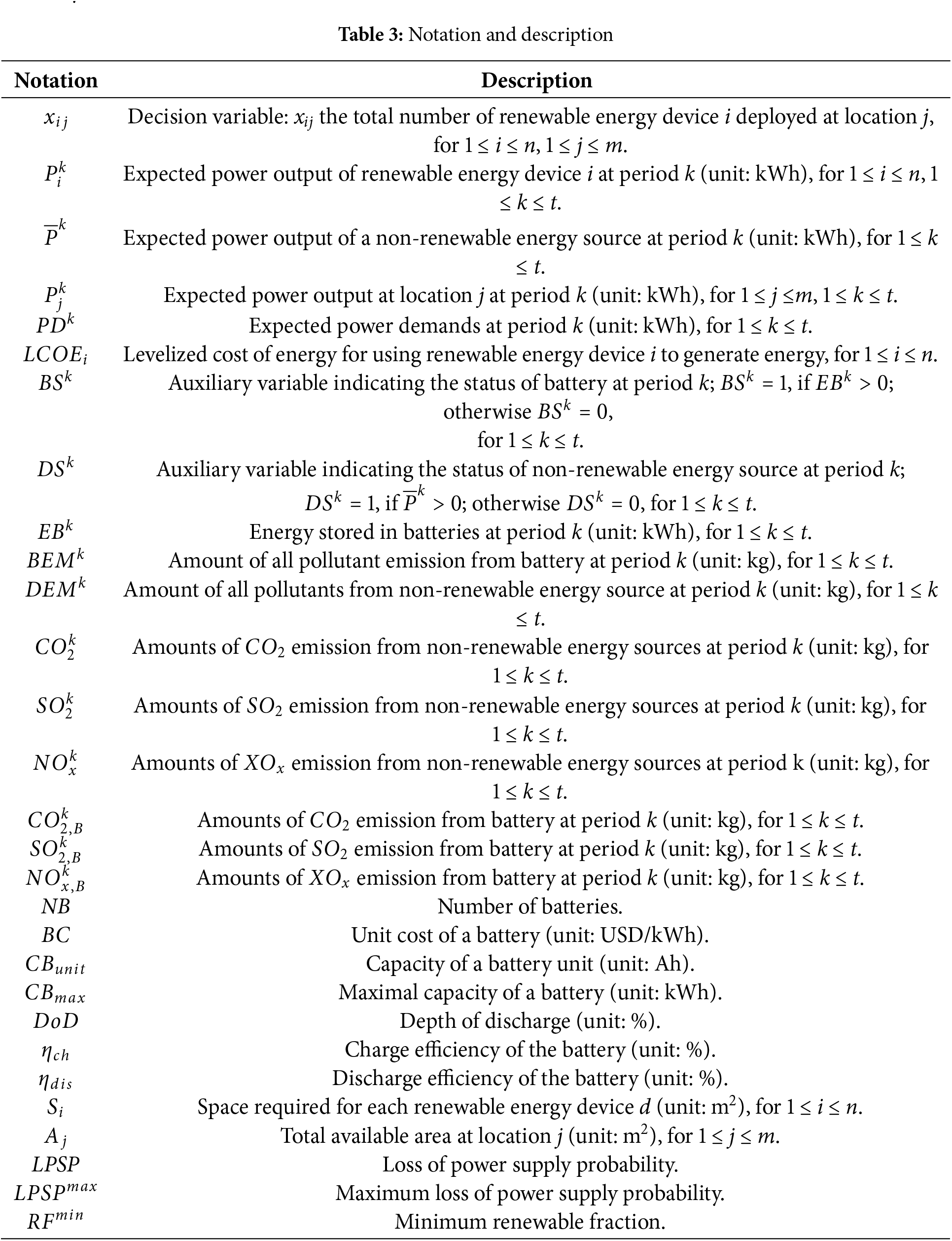
Fig. 1 depicts the three primary energy sources (renewable, non-renewable, and energy storage) that supply electricity to four institutional load types (hotels, factories, universities, and hospitals). Renewable energy sources include solar panels and wind turbines, while diesel generators represent the non-renewable component. Batteries serve as the energy storage mechanism. This integrated system forms the basis for the optimization model described in this study.

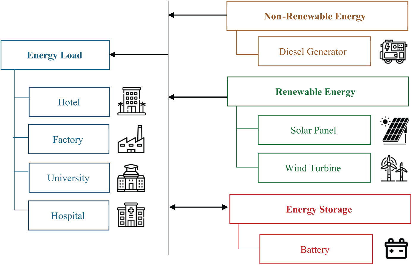
Figure 1: Schematic diagram of the hybrid renewable energy system

2.2 Mathematical Model

We enhance the mathematical model originally formulated by Trihardani et al. [12], which now integrates additional considerations highlighted by various researchers in the field [15–19]. The studied model incorporates several critical considerations, including pollutant emissions and system reliability, with the latter quantified based on the probability of power supply loss as delineated in previous research by Ramli et al. [24] and Kharrich et al. [16]. Our model also defines the renewable energy fraction, a concept that has been extensively explored and validated in the studies by Çetinbaş et al. [19] and Kharrich et al. [16] as the proportion of total energy derived from renewable sources. Additional practical considerations in the HRES focus on the efficiency of battery charging and discharging processes, as well as the minimal capacity required for each battery unit—factors that are essential for optimizing system performance and sustainability. These battery-related aspects have been extensively studied and are influenced by the research of Niknam et al. [22], Shin et al. [23], and Rekioua [21], which provide foundational insights into optimizing battery usage to enhance the efficiency and viability of renewable energy allocations.

The objective is to strategically deploy renewable energy devices across available locations to achieve optimal arrangement within a specific period k. The decision variables xij in the proposed problem are the quantities of renewable energy device i placed at available location j. The objective is to minimize the operation cost and pollutant emission fees by adopting the weighted sum method to convert the multi-objective problem into a single objective function in Eq. (1). The operation cost represented in Eq. (2) includes the cost associated with batteries, as calculated by the number of batteries and the unit cost of the batteries, and the cost of energy generation, as calculated by summing up the levelized cost of energy for all devices across all locations and periods. Eq. (3) defines the total pollutant emission fees from both battery storage and non-renewable energy sources, accounting for whether the batteries or non-renewable energy sources are in use at any given period.

The objective function and its components are formulated as follows:

Minimize wF1+(1−w)F2(1)

where:

•   w is the weighting factor (0 ≤ w ≤ 1) balancing the importance between cost and environmental impact

•   F1 represents the total operational cost

•   F2 represents the environmental impact cost

The operational cost component is defined as:

F1=(NB∗BC)+(∑i=1n∑j=1m∑k=1txij∗Pik∗LCOEi)(2)

where:

•   NB × BC represents the total battery cost

•   xij is the total number of renewable energy device i deployed at location j

•   Pik is the expected power output (in kWh) of renewable energy device i during period k

•   LCOEᵢ is the Levelized cost of energy for using renewable energy device i to generate energy

The environmental impact component is defined as:

F2=(∑k=1tEBk∗BEMk)+(∑k=1tP¯k∗DEMk)(3)

where:

The first term represents battery-related emissions:

•   EBk is the energy stored in batteries at period k

•   BEMk is the amount of all pollutant emission from battery at period k

The second term represents non-renewable energy emissions:

•   P¯k is the expected power output of a non-renewable energy source at period k

•   DEMk is the amount of all pollutants from non-renewable energy source at period k

Constraints governing energy generation are delineated in Eq. (4), which ensures that the total power output at each location j during period k precisely equals the sum of the outputs from all devices deployed therein. Eq. (5) ensures that the power demand at any given period k is met by the combined outputs of renewable, non-renewable, and battery systems. Eq. (6) formalizes the constraint that energy consumption aligns with demand, stipulating that the energy stored in batteries at period k equals the energy accumulated at period k − 1 plus the power output at period k, minus the power demands at that same time. Notably, this equation also accounts for the charging and discharging efficiencies of the batteries, as defined in the studies by Niknam et al. [22] and Shin et al. [23], ensuring a precise adjustment for energy conservation and efficiency in system operations. Eqs. (7) and (8) quantify the pollutant emissions from battery systems and non-renewable energy devices, respectively, by aggregating the emissions of CO2, SO2, and NOx from the battery system at period k and summing the pollutants emitted by non-renewable energy sources. Based on the research by Elattar et al. [15], this formulation provides a comprehensive method for accurately assessing environmental impacts associated with energy production at different stages of the system’s operation. Eqs. (9) and (10) calculate the requisite number of batteries by integrating a formula that considers power requirements and battery capacity. Specifically, Eq. (9) ensures that the energy stored at any time does not surpass the total capacity of the batteries, while Eq. (10) quantifies the number of batteries required based on system demand and individual battery capacities, as delineated in the research from Rekioua [21]. Eq. (11) ensures that the total deployment area remains within each location’s spatial boundaries. Eq. (12) ensures that the Loss of Power Supply Probability (LPSP) remains below a predefined maximum allowable threshold, enhancing system reliability. Concurrently, Eq. (13) has been adopted from the work of Ramli et al. [24]. Eq. (14) derived from the work of Ramli et al. [24], guarantees that the proportion of the system’s energy derived from renewable sources exceeds a designated minimum threshold, thus ensuring the sustainability and effectiveness of the energy system. Eqs. (15) and (16) define the auxiliary variables BSk, which indicate the operational status of the batteries at period k; specifically, these variables denote whether the batteries are active, based on the condition that the energy stored exceeds zero. Eqs. (17) and (18) define the auxiliary variables DSk, which signify the operational status of non-renewable energy devices at period k; these variables specifically indicate whether the devices are active, contingent upon the satisfaction of energy demands. The following is the proposed mixed integer programming (MIP) model:

Pjk=∑i=1nxij∗Pik,∀j,k(4)

PDk≤∑j=1mPjk+P¯k+EBk,∀k(5)

EBk=EBk−1+ηch(∑j=1mPjk+P¯k)Δk−(1ηdis)PDkΔk,∀k(6)

BEMk=(CO2,Bk+SO2,Bk+NOx,Bk)BSk,∀k(7)

DEMk=(CO2k+SO2k+NOxk)DSk,∀k(8)

EBk≤CBmax∗NB,∀k(9)

NB=ENT[∑k=1tPDkV∗DOD∗ηdih∗CBunit](10)

∑i=1nxij∗Si≤Aj,∀j(11)

LPSP≤LPSPmax(12)

LPSP=∑k=1t(PDk−∑j=1mPjk+P¯k+EBk)∑k=1tPDk(13)

∑k=1tP¯k≤(1−RFmin)∑j=1m∑k=1tPjk(14)

EBk−BSkM≤0,∀k(15)

EBk+(1−BSk)M>0,∀k(16)

P¯k−DSkM≤0,∀k(17)

P¯k+(1−DSk)M>0,∀k(18)

xij≥0,∀i,j(19)

A toy example following the input file format based on the language MiniZinc [25] is created and shown in Fig. 2. To better illustrate the problem structure, this example presents the following components:

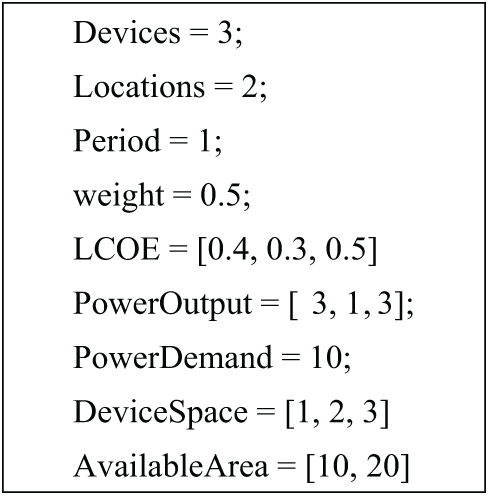
Figure 2: A toy example

•   Problem parameters

This example presents a simplified scenario with three devices (n = 3) that can be placed across two locations (m = 2). The problem is further simplified by considering just a single period and uses an objective weight (w) of 0.5 to balance different optimization goals.

•   Device specification

The three devices each have unique characteristics. Their Levelized Cost of Energy (LCOE) values are 0.4, 0.3, and 0.5, respectively. During the single period, they generate expected power outputs of 3, 1, and 3 kWh. Each device also requires specific space for installation: 1 square meter for device 1, 2 square meters for device 2, and 3 square meters for device 3.

•   Location constraints

The two installation locations have different space availabilities. Location 1 offers 10 square meters of space, while location 2 has 20 square meters available. The system must meet a total power demand of 10 kW.

•   Solution representation

The solution is represented as {(0, 0), (0, 1), (3, 3)}, where each tuple shows how a device type is distributed across the two locations. The first tuple (0, 0) indicates that device type 1 is not installed in either location. The second tuple (0, 1) shows that one device of type 2 is installed in location 2. The third tuple (3, 3) indicates that three devices of type 3 are installed in both locations.

•   Solution evaluation

This configuration generates a total power output of 19 kW. This comes from two sources: the single type 2 device contributes 1 kW (1 × 1 kW), and the six type 3 devices contribute 18 kW ((3 + 3) × 3 kW). The complete solution achieves an objective value of 255.59.

This paper incorporates several fundamental assumptions aligned with current HRES optimization research [26]. These assumptions are essential for creating manageable models while maintaining practical relevance:

•   Uncertainty Management: Following established practices in HRES optimization, discrepancies between predicted and actual weather data are disregarded. This assumption allows us to focus on developing optimization techniques that can handle the general variability in energy production and demand patterns.

•   Economic and Sizing Evaluation: The power generation calculation for solar panels considers primary factors such as hours of sunlight and device efficiency. This simplification aligns with common approaches in economic evaluation and system sizing optimization, while acknowledging that real-world performance may be affected by additional variables.

•   System Performance: Variations between forecasted electricity demand and actual data are streamlined to focus on general trends rather than real-time fluctuations. This approach follows standard practices in system interference management, enabling us to model the seamless integration and operation of system components.

These assumptions are crucial for deriving practical solutions while maintaining computational feasibility. Future research could validate these assumptions through empirical data and testing, particularly in:

•   Incorporating more sophisticated uncertainty modeling for renewable energy sources

•   Developing dynamic approaches to economic and sizing evaluation

•   Enhancing system interference management through real-time data integration

Such extensions would further strengthen the practical implementation of HRES optimization across various institutional settings.

3  IHHO with Multiple Neighborhood

3.1 Improved Harris Hawks Optimization

A review of recent HRES optimization literature reveals several prevalent metaheuristic approaches. Particle Swarm Optimization (PSO) has been applied by Soheyli et al. [17] and Gupta et al. [20], while Elattar et al. [15] implemented the Salp Swarm Algorithm (SSA). Harris Hawks Optimization (HHO) has been employed by Kharrich et al. [16] and Çetinbaş et al. [19], with additional methods like Sailfish Optimization explored by Li et al. [18]. Çetinbaş et al. [19] demonstrated HHO’s superiority over PSO and SSA, prompting our choice of HHO. However, HHO’s tendency for premature convergence necessitates improvement. In 2022, Gezici et al. [27] addressed this limitation with their Improved HHO (IHHO).

IHHO refines random parameter determination, enhances solution generation strategies, and streamlines the decision mechanism from six steps to four. This simplification and modified approach to random parameters aim to boost algorithm performance. We adopt IHHO in our study to tackle the studied optimization problems.

The flowchart in Fig. 3 illustrates the comprehensive structure of the Improved Harris Hawks Optimization (IHHO) algorithm. Harris Hawks Optimization (HHO) is a population-based metaheuristic algorithm that simulates the cooperative hunting and chasing behavior of Harris hawks in nature. IHHO enhances this concept by improving exploration and simplifying exploitation strategies. In Fig. 3, the main processes of IHHO include:

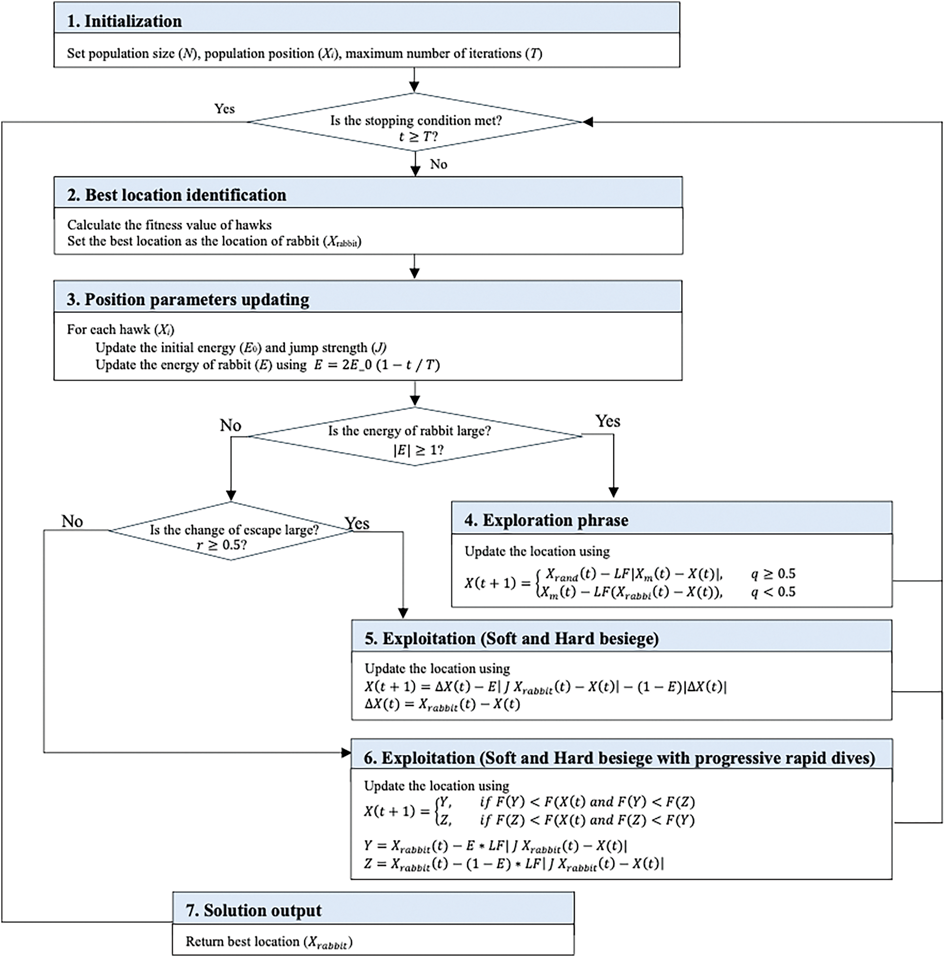
Figure 3: Flowchart of IHHO

1.    Initialization: This step sets the algorithm’s foundation. It defines the population size (N), iteration number (T), and initializes the random population Xi (i = 1, 2, … , N). This diverse initial population ensures a broad search starting point.

2.    Best Location Identification: The algorithm calculates fitness values for all hawks and identifies Xrabbit as the current optimal solution. This serves as a reference for other hawks in subsequent steps.

3.    Position Parameter Updating: For each hawk, the algorithm updates the initial energy E0 and jump strength J. It then updates energy E, determining the transition between exploration and exploitation phases.

4.    Exploration Phase: When |E| ≥ 1, the algorithm explores. IHHO employs Levy flight distributions here, enhancing its ability to discover promising regions that random searches might overlook.

5.    Exploitation Phase (Soft and Hard Besiege): For |E| < 1 and r ≥ 0.5, the algorithm exploits. IHHO combines soft and hard besiege strategies into a single, efficient approach, allowing smooth transition between different local search intensities.

6.    Exploitation (Soft and Hard Besiege with Progressive Rapid Dives): When |E| < 1 and r < 0.5, this aggressive exploitation phase triggers. It combines soft and hard besiege with progressive rapid dives, refining solutions in promising areas.

7.    Solution Output: After meeting termination criteria, the algorithm outputs the best solution (Xrabbit), representing the optimized result.

E=2E0(1−tT)(20)

X(t+1)={Xrand(t)−r1|Xrand(t)−2r2Xt|,q≥0.5Xrabbit(t)−Xm(t)−r3(LB+r4(UB−LB)),q<0.5(21)

X(t+1)=ΔX(t)−E|JXrabbit(t)−X(t)|−(1−E)|ΔX(t)|(22)

ΔX(t)=Xrabbit(t)−X(t)(23)

X(t+1)={Y,ifF(Y)<F(X(t)andF(Y)<F(Z)Z,ifF(Z)<F(X(t)andF(Z)<F(Y)(24)

Y=Xrabbit(t)−E∗LF|JXrabbit(t)−X(t)|(25)

Z=Xrabbit(t)−(1−E)∗LF|JXrabbit(t)−X(t)|(26)

3.2 Multiple-Neighborhood Enhanced Harris Hawks Optimization

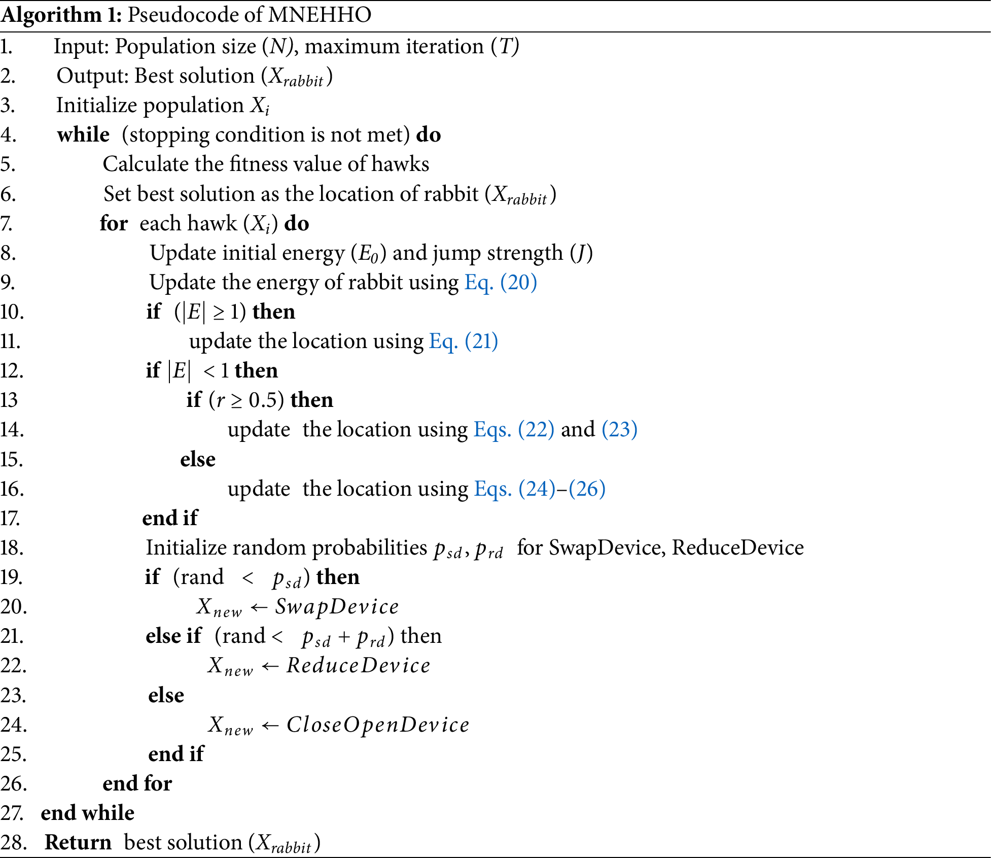
We enhance the Improved Harris Hawks Optimization (IHHO) algorithm [27] by incorporating multiple neighborhood structures, enabling more effective HRES solution space exploration. Algorithm 1 presents the pseudocode of our improved approach. This enhancement maintains IHHO’s core optimization process while adding structured local search through multiple neighborhoods, particularly beneficial for the complex solution space of HRES allocation problems.

3.3 Encoding and Initialization

Considering the simplicity of encoding, we represent each solution as an n×m matrix. Each element in this matrix denotes the quantity of a device i deployed in location j. However, large problem instances generate an expansive search space when based directly on the decision variables xij. To tackle this challenge effectively, we implement strategies to reduce the search space without sacrificing solution quality. These strategies aim to streamline our approach while preserving all potential optimal solutions.

We reduce the quantity of devices in each location by simultaneously considering two key factors: the expected power demand and the available area. We introduce a new parameter (αij) constraints the upper bounds of each decision variable in Eq. (27).

αij=min(⌈PDkpik⌉,⌊AjSi⌋),∀i,j(27)

This parameter combines the expected power demands and space constraints, allowing for a more efficient encoding in our metaheuristic algorithm. By limiting each decision variable xij to its corresponding αij, we significantly shrink the search space while retaining all feasible solutions.

As for the initial solution, we employ two strategies: random and greedy. The random strategy, which quickly produces diverse solutions, operates as follows: For each location, we iteratively select a device at random and increase its quantity by one until the expected power demand is met. We then verify that the total area occupied by devices at each location does not exceed the available space. The greedy strategy follows a similar process but prioritizes cost-effectiveness. It selects devices based on their levelized cost of energy (LCOE) and power output, favoring those with lower LCOE and higher output. This approach aims to satisfy power demands more efficiently while still adhering to spatial constraints.

3.4 Multiple Neighborhoods

The effectiveness of our approach relies heavily on three specialized neighborhood structures, each designed to address specific aspects of the HRES optimization problem. We consider three different atomic neighborhoods, starting with SwapDevice (SD).

3.4.1 SwapDevice (SD) Neighborhood

We introduce the SwapDevice (SD) neighborhood, a specialized structure designed to optimize cost efficiency by strategically exchanging device quantities within a single location. This neighborhood is characterized by three key elements: a location l∈{1,…,m}, and two devices d1 and d2, d1,d2∈{1,…,n}. The SD ⟨l,d1,d2⟩ move swaps the quantities of two devices at location l, where

•   l is selected as the location with the largest available space, addressing potential installation constraints

•   d1 represents the device with non-zero quantity having the highest unit cost (LCOE/power output ratio)

•   d2 identifies the device with non-zero quantity having the lowest unit cost

To illustrate the effectiveness of this neighborhood structure, consider Toy Example (Fig. 2). An initial solution {(0, 0), (0, 1), (3, 3)} with an objective value of 255.59 transforms to {(0, 3), (0, 1), (3, 0)} after applying the SD ⟨l=2,d1=3,d2=1⟩ move, reducing the objective value to 255.14, demonstrating a measurable improvement through strategic device quantity redistribution.

The SwapDevice neighborhood design carefully balances practical consideration with efficiency optimization through three key mechanisms:

•   Prioritizing location with larger available areas to mitigate space limitations

•   Selecting devices based on unit cost differentials to optimize power demand satisfaction

•   Exchanging quantities between high-cost devices to improve overall economic efficiency

This approach enables systematic exploration of the solution space for cost-effective HRES configuration while maintaining all system constraints, particularly power putout requirements and space limitations.

3.4.2 ReduceDevice (RD) Neighborhood

Our second atomic neighborhood, the ReduceDevice (RD), focuses on optimizing space utilization and meeting expected power demand efficiently by reducing device quantities within a single location. Similar to SwapDevice, this neighborhood structure comprises three critical elements: a location l, a device dr to be reduced, and a reduction quantity qr, where l ∈ {1, … , m} and dr ∈ {1, … , n}.

The RD ⟨lr,dr,qr⟩ moves systematically reduces the quantity of device dr at location lr by qr units, with the following selection criteria:

•   lr is identified as the location with the smallest available space to optimize constrained areas

•   dr is selected as the device with non-zero quantity having the highest unit cost

•   qr is calculated as the integer value of the reduction amount determined by dividing the excess total power output over expected demand by the expected power output of device dr

To demonstrate this neighborhood’s effectiveness, consider our Toy Example, {(0, 0), (0, 1), (3, 3)} with an objective value of 255.59 transforms to {(0, 0), (0, 1), (2, 3)} after applying the RD ⟨lr=1,dr=3,qr=1⟩ move, reducing the objective value to 254.8. In this case, location 1 (with an area of 10) is selected, and device 3 (with the highest unit cost) is chosen for reduction.

The constraints and rationale governing this neighborhood design are grounded in practical considerations and efficiency optimization:

•   The prioritization of smaller areas addresses potential space constraints in more limited locations

•   The selection strategy based on the highest unit cost optimizes the balance between power generation and electricity demand

•   The move executes only when power generation exceeds demand, ensuring reduction to the minimum threshold that satisfies electricity requirements

Importantly, this move is not performed if power generation is insufficient or if the reduction would compromise power generation adequacy. Additionally, since increasing device quantities cannot improve the objective value, such actions are excluded from this neighborhood structure. This approach enables targeted exploration of the solution space, focusing on cost-efficient device allocation while maintaining operational feasibility and meeting power demands.

3.4.3 CloseOpenDevice (COD) Neighborhood

Our third atomic neighborhood, CloseOpenDevice (COD), is designed to strategically replace one type of power generation device with another within a single location, optimizing cost efficiency while maintaining power output. This neighborhood is identified by three critical elements: the location lco, the device to be removed dc, and the device to be added do.

The COD ⟨lco,dc,do⟩ move implements a sophisticated transformation where:

•   The quality of device dc at location lco is reduced to zero

•   The quantity of device do at the same location is increased to precisely meet the power output previously provided by device dc

•   lco is assigned to the area with the smallest available space

•   dc is selected as the device with zero quantities at location lco having the lowest unit cost

To illustrate the effectiveness of this. Neighborhood structure, consider our Toy Example with an initial solution of {(0, 0), (0, 1), (2, 3)} and an objective value of 254.8. After applying the COD ⟨lco=1,dc=1,do=3⟩ move, the solution becomes {(2, 0), (0, 1), (0, 3)}, reducing the objective value to 254.5. This demonstrates a measurable improvement through strategic device substitution.

The design principles underlying the COD neighborhood align with those of the ReduceDevice neighborhood, particularly in prioritizing locations with smaller areas to address space constraints in limited locations. Additionally, this neighborhood implements a dual selection strategy:

•   Selecting dc (device to remove) based on the highest unit cost to eliminate less cost-efficient power generation

•   Selecting do (device to add) based on lowest unit cost to introduce more economical apower generation

This targeted approach enables systematic exploration of the solution space focused on economic efficiency while maintaining the required power generation capacity, ensuring operational constraints remain satisfied.

3.5 Overall Time Complexity

Since MNEHHO is built upon IHHO, which has a complexity of O(N×T×D+T×N) per iteration [27] where D represents the problem dimension (m×n in our case, with m locations and n devices), we need to analyze the additional computational cost introduced by the multiple neighborhood structures. Each neighborhood operation (SD, RD, and COD) requires O(m+n) operations.

For T iterations and population size N, the total complexity becomes:

O(N×T×(m×n)+T×N+T×N×(m+n))

Since m×n dominates m+n, the overall time complexity can be simplified to: O(T×N×m×n).

This indicates that MNEHHO maintains the same order of complexity as IHHO while incorporating the additional neighborhood search capabilities. Our experimental results on small-scale instances (Table 4) validate this analysis, showing only modest increases in computational time while achieving significant improvements in solution quality.

4  Experimental Analysis

4.1 Experimental Setting

This study utilizes artificially generated datasets based on real-world energy demand pattern observations. The purpose of these datasets is to evaluate the performance of the proposed optimization model under practical energy demand scenarios.

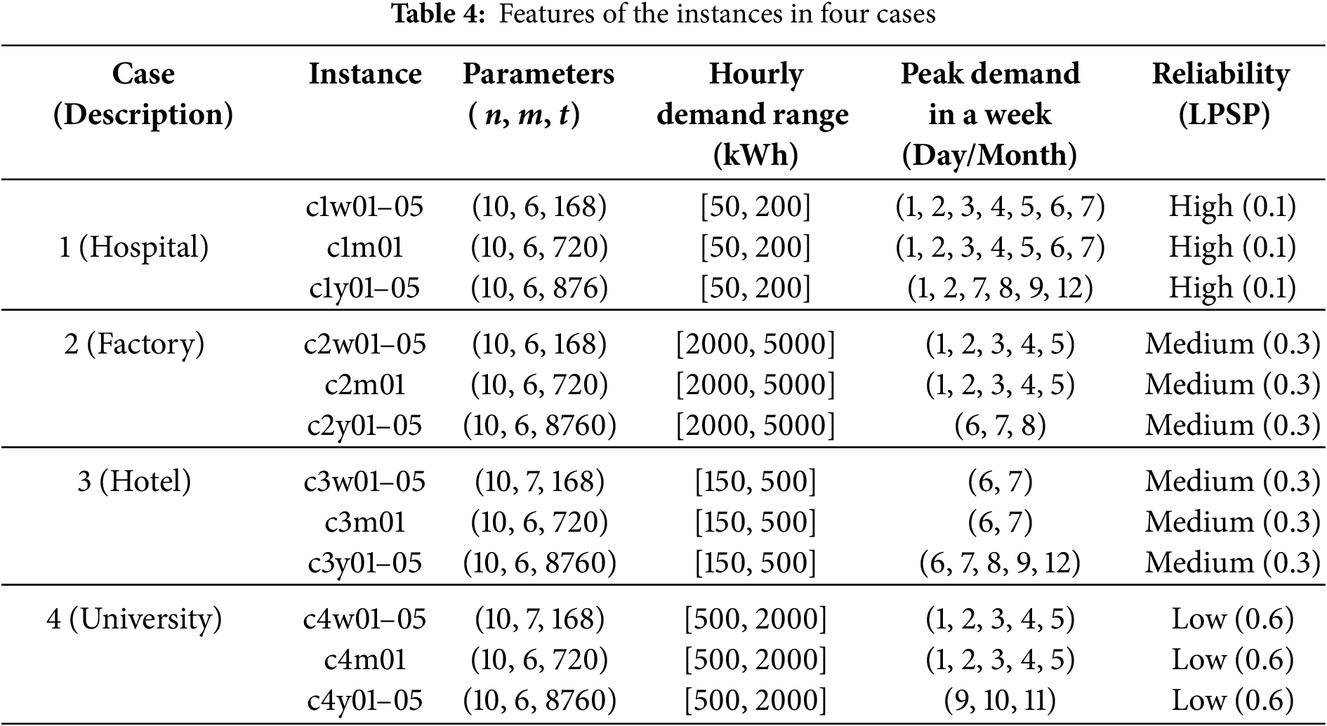
We analyze four cases representing different types of facilities: hospitals, factories, hotels, and universities. Each case includes 11 instances varying in time horizons (5 weekly, 1 monthly, and 5 yearly). The critical parameters for each instance are the number of renewable energy devices (n), available locations (m), time periods (t), hourly demand range (kWh), peak demand days in a week, and reliability requirements (LPSP). Table 1 summarizes the instance features, and Fig. 4 illustrates the hourly demands for each case, providing a visual representation of their unique consumption patterns over time.

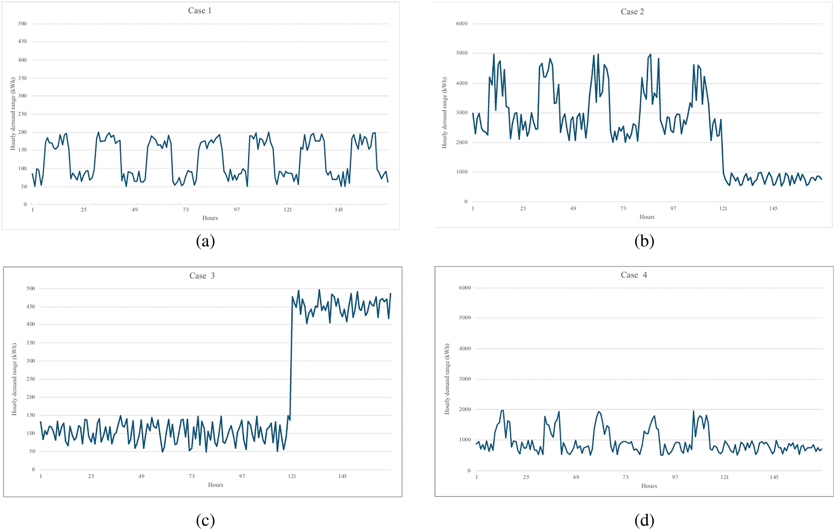
Figure 4: Hourly demand for four cases. (a) hospital (b) factory (c) hotel (d) university

The following paragraphs describe the specific characteristics of each case:

Hospital (Case 1) instances have 10 renewable energy devices and 6 available locations. The hourly demand range is moderate (50~200 kWh), with consistent peak weekly demand. It requires high reliability (LPSP 0.1). As shown in Fig. 4a, the energy demand pattern shows regular daily cycles with slight variations, reflecting the constant operation of medical facilities. Available locations for renewable energy deployment include rooftops, parking structures, open courtyards, facades, green spaces/gardens, and service and maintenance areas.

Factory (Case 2) has the highest hourly demand range (2000~5000 kWh). Peak demands are primarily on weekdays for weekly and monthly instances, shifting to weekends for yearly instances. It has medium reliability requirements (LPSP 0.3). Fig. 4b demonstrates clear distinctions between operational and off-hours, with significantly higher demand during weekday working hours. Available locations for renewable energy deployment include rooftops, parking lots, unused land, facades, green spaces, and adjacent warehouses.

Hotel (Case 3) instances have a moderate demand range (150~500 kWh). Peak demands occur on weekends, with additional peak days in yearly instances. It has medium reliability requirements (LPSP 0.3). As illustrated in Fig. 4c, the energy demand pattern shows daily fluctuations with higher demand in the evenings and nights and notable increases during weekends. Available locations for renewable energy deployment include rooftops, balconies, front porches, outdoor barbecue areas, decks, outdoor fireplaces, and water ponds.

University (Case 4) instances have a broad demand range (500~2000 kWh). The peak demand is on weekdays for weekly and monthly instances, shifting to different months for yearly instances. It has the lowest reliability requirements (LPSP 0.6). Fig. 4d exhibits clear differences between weekdays and weekends, with higher demand during daytime hours on weekdays and lower, more consistent demand on weekends. Available locations for renewable energy deployment include rooftops, parking lots, campus grounds, sports fields, water bodies, green spaces, and building facades.

These diverse energy demand patterns and varied location options across different facility types provide a comprehensive test bed for evaluating the robustness and adaptability of the proposed optimization model in various real-world scenarios.

For all scenarios, the optimization models are solved with IBM ILOG CPLEX Optimization Studio 20.10, using a personal computer powered by Intel Core i7-14700 processor (running at 2.10 GHz) and 32 GB RAM.

4.2 Results and Analysis

Our experimental analysis demonstrates the effectiveness of integrating multiple operational constraints with an enhanced optimization algorithm. The results validate three key aspects of our contribution: (1) the practicality of simultaneously considering multiple operational constraints, (2) the effectiveness of our multiple neighborhood structures in improving solution quality, and (3) the adaptability of our approach across different institutional settings with varying reliability requirements.

We present our results in two parts. Section 4.2.1 validates our approach using small-scale random instances where optimal solutions can be obtained through exact methods, establishing the effectiveness of our algorithmic improvements. Section 4.2.2 demonstrates the practical applicability of our approach through comprehensive testing across four real-world scenarios: hospitals, factories, hotels, and universities. These scenarios represent different operational contexts with varying reliability requirements, energy demand patterns, and operational constraints, providing robust validation of our integrated approach.

The results consistently show that our integrated consideration of multiple operational constraints, combined with the proposed multiple neighborhood structures, leads to significant improvements in both solution quality and practical effectiveness. The improvements range from 36% to 46% across different scenarios, with particularly strong performance in cases with stringent reliability requirements.

4.2.1 Computational Results on Small-Scale Random Instances

Table 5 presents the computational results for small-scale random instances. In this table, LB represents the objective value obtained by the CPLEX solver within a time limit of 3600 s. The Gap indicates the relative difference between the lower bound and the solution found by each metaheuristic algorithm. Time denotes the computational time in seconds required by each algorithm to obtain its solution.

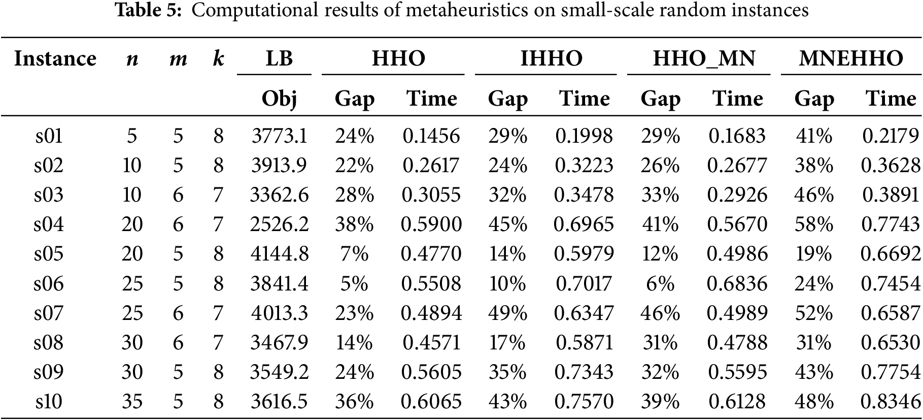
These instances vary in size, with the number of devices (n) ranging from 5 to 35, locations (m) from 5 to 6, and time periods (k) from 7 to 8. Overall, the results demonstrate that all four algorithms can solve these instances efficiently, with computational times consistently under one second.

In terms of solution quality, MNEHHO generally outperforms the other three algorithms across most instances. This superior performance is particularly evident in instances s05 and s06, where MNEHHO achieves gaps of 19% and 24%, respectively, compared to more significant gaps obtained by the basic HHO (7% and 5%). The improvement in solution quality can be attributed to the incorporation of multiple neighborhood structures, which enhances the algorithm’s ability to explore diverse solution spaces.

When examining computational efficiency, we observe that execution times increase with problem size, as expected. For example, instance s01 (n = 5, m = 5) requires approximately 0.15–0.22 s across all algorithms, while instance s10 (n = 35, m = 5) needs 0.61–0.83 s. Notably, while MN-enhanced variants (HHO_MN and MNEHHO) generally require slightly more computational time, the increase is modest—typically 15%–30% longer than their base versions.

The impact of problem size on solution quality shows exciting patterns. For smaller instances (s01–s03), the gap differences among algorithms are relatively modest. However, as the problem size increases, particularly in instances s07–s10, the performance gap between algorithms becomes more pronounced. This suggests that the multiple neighborhood strategy becomes more beneficial as problem complexity increases.

In terms of algorithmic stability, both IHHO and MNEHHO demonstrate more consistent performance across different instances compared to their HHO counterparts. This is evidenced by smaller variations in their gap values, particularly in mid-sized instances (s04–s07). This improved stability can be attributed to the enhanced exploration mechanisms in the improved versions.

To summarize, our analysis reveals that while all algorithms can efficiently handle small-scale instances, MNEHHO emerges as the most effective approach, particularly for larger instances within this category. The multiple neighborhood strategy proves particularly valuable when dealing with increased problem complexity, though it comes with a modest computational overhead. These findings suggest that MNEHHO would be particularly suitable for applications where solution quality is prioritized over minimal computation time.

4.2.2 Computational Results and Practical Implications for Different Facility Types

Tables 6–9 present a comprehensive quantitative analysis comparing the performance of metaheuristic algorithms across different power demands. To ensure robust statistical validation, we conducted 100 independent runs for each algorithm configuration, analyzing results across weekly (w), monthly (m), and yearly (y) time scales. For example, case 1 includes weekly instances c1w01–c1w05, a monthly instance c1m01, and yearly instances c1y01–c1y05.

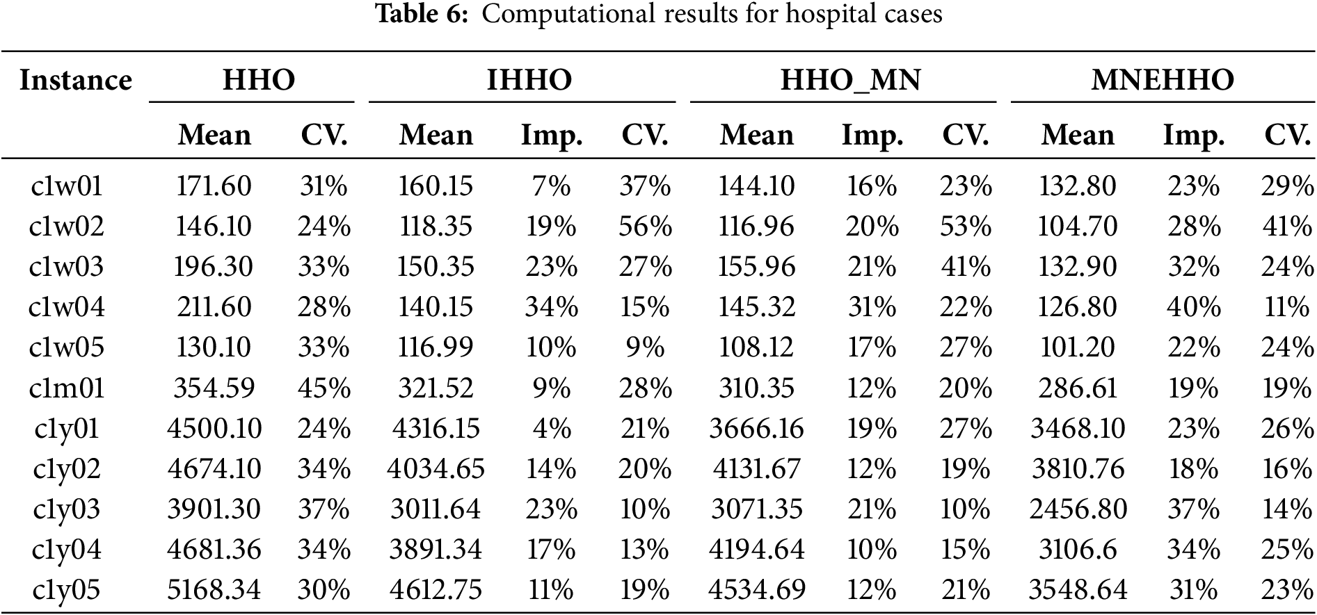
To establish clear quantitative benchmarks, we analyze three key performance metrics: Mean, CV (coefficient of variance), and Imp. (improvement). The Mean represents the average objective value obtained from 100 independent runs—lower values indicate better solutions as our goal is to minimize both the levelized cost of energy (LCOE) and pollutant emissions costs. The CV measures the algorithm’s stability, where a lower value demonstrates more consistent performance across multiple runs. The improvements show the percentage improvement of each algorithm compared to the original HHO. This metric helps quantify the progress made by the IHHO, HHO_MN, and MNEHHO algorithms concerning the baseline HHO performance.

Table 6 presents the computational results for hospital cases, comparing the performance of HHO, IHHO, HHO_MN, and MNEHHO across different time periods. MNEHHO achieves superior results in short-term instances such as c1w01, with a mean objective value of 132.80, representing improvements of 22.6% over HHO (171.60), 17.1% over IHHO (160.15), and 7.8% over HHO_MN (144.10). This improvement can be attributed to the incorporation of multiple neighborhood structures.

MNEHHO demonstrates competitive stability, with CV values ranging from 11% to 41% for short-term instances. In contrast, HHO exhibits stable performance with a CV between 24% and 45%, while IHHO shows greater variability, with a CV reaching up to 56%. The improvement between the algorithms becomes more pronounced as the instance size increases. In the long-term instance c1y05, MNEHHO achieves a mean objective value of 3548.64, which is significantly better than HHO (5168.34), IHHO (4612.75), and HHO_MN (4534.69).

To further analyze the impact of incorporating the multiple neighborhood (MN) strategy, Table 6 demonstrates that HHO_MN outperforms HHO by 10% to 31% (with an average improvement of 17.4%), while MNEHHO surpasses IHHO by 18% to 40% (with an average improvement of 28%). These results underscore the effectiveness of the MN strategy in enhancing the performance of both the HHO and IHHO algorithms.

Detailed statistical analysis across all hospital cases reveals three key performance aspects. First, in terms of solution quality, MNEHHO demonstrates consistent superiority by achieving improvements ranging from 23% to 40% compared to the baseline HHO algorithm. Second, regarding computational stability, the algorithms exhibit distinct patterns in their coefficient of variation (CV). The baseline HHO shows an average CV of 32.1% with a standard deviation of 6.2%, while IHHO achieves better stability with an average CV of 23.1% (σ = 13.4%). The multiple neighborhood variants demonstrate comparable stability, with HHO_MN averaging 24.5% (σ = 10.8%) and MNEHHO showing the most consistent performance with an average CV of 22.7% (σ = 8.5%). Third, examining performance scaling reveals that the improvement margin correlates positively with problem size, with the most substantial enhancements of up to 40% observed in yearly instances, indicating MNEHHO’s effectiveness in handling larger-scale problems.

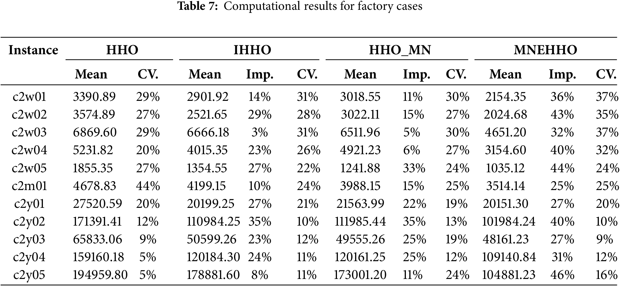
Table 7 analyzes the computational results for hospital cases with medium reliability requirements (LPSP = 0.3), revealing distinct patterns in the effectiveness of the algorithms.

Regarding solution quality, MNEHHO excels in addressing the long-term energy requirements typical of hospital operations. For instance, in case c2w02, MNEHHO achieves a mean objective value of 2024.68, which represents a significant improvement over the HHO. The performance improvement increases to 26.8% in extended period cases such as c2y03, where MNEHHO’s mean value of 48161.23 reflects its superior capability to optimize energy allocation for long-term healthcare facilities.

The stability patterns of algorithms are a notable feature of the results. The HHO and IHHO algorithms exhibit relatively low variability, with CV values averaging 21%. In contrast, HHO_MN (average CV of 23%) and MNEHHO (average CV of 24%) demonstrate comparable stability while managing more complex operational constraints within hospitals. This indicates that the algorithms maintain their reliability even when addressing the increased computational complexity associated with healthcare facility challenges.

The improvement percentages in hospital scenarios are particularly noteworthy; for instance, consider c2y05. HHO_MN achieves an 11% improvement over the HHO algorithm, while MNEHHO achieves a 46% improvement. In contrast, MNEHHO demonstrates a more substantial 46% enhancement, underscoring the effectiveness of integrating the improved HHO mechanism with a multiple-neighborhood strategy for extended planning periods in hospital environments.

These significant gains suggest that the multiple neighborhood strategy is particularly effective in tackling the unique challenges associated with energy optimization in healthcare facilities, especially under medium reliability requirements.

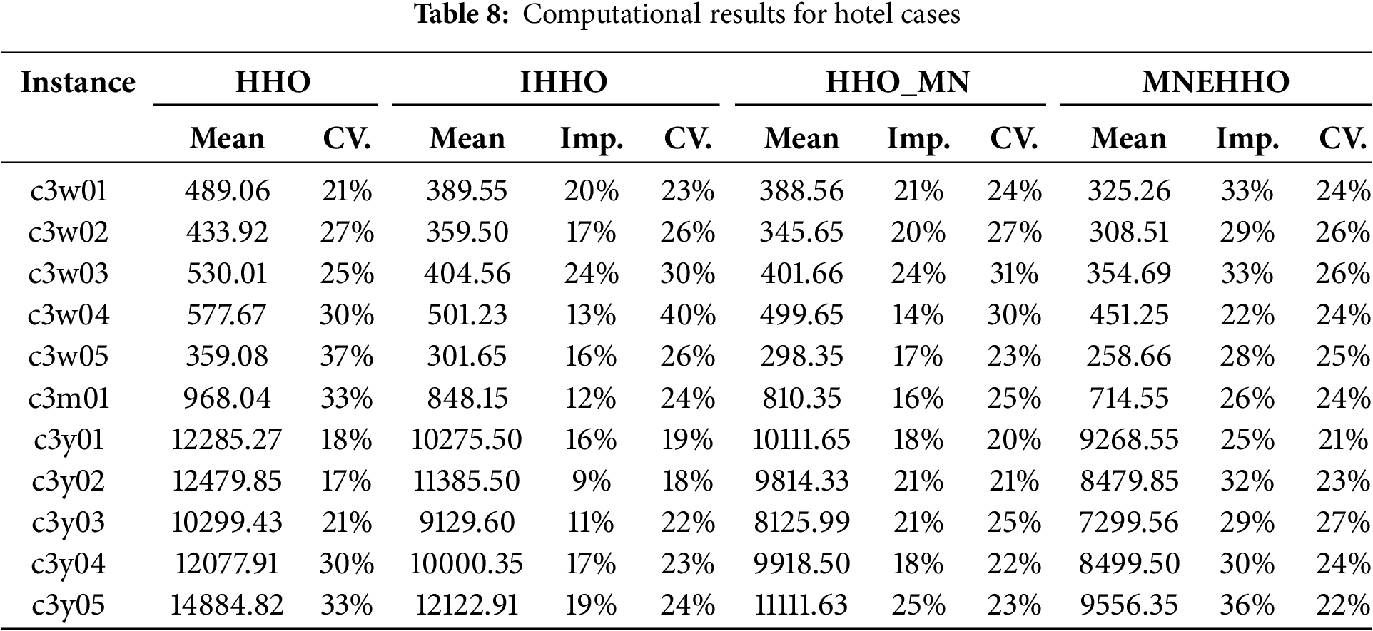
The results presented in Table 8 illustrate the computational performance for hotel cases. It is evident that MNEHHO consistently achieves the highest quality of solutions in managing hotel-specific energy demands. This is particularly noticeable in case c3w02, where MNEHHO attains a mean objective value of 308.51, showing improvements of 28.9% over HHO (433.92), 14.2% over IHHO (359.50), and 10.7% over HHO_MN (345.65). The advantages of MNEHHO become especially pronounced over longer planning horizons, as demonstrated in case c3y03, where its mean value of 7299.56 indicates a superior capability in long-term hotel energy allocation.

Examining the stability metrics reveals intriguing patterns across all algorithms. HHO exhibits relatively higher variability, with CV values ranging from 18% to 33% (averaging 26%). In contrast, the Improved Harris Hawks Optimization (IHHO) and HHO_MN show slightly better consistency, with CV values ranging from 19% to 40% (averaging 25%) and 20% to 31% (averaging 25%), respectively. Meanwhile, MNEHHO maintains steady performance levels, with an average CV value of 24%, indicating reliable optimization across various hotel operational scenarios.

The test cases demonstrate performance enhancements resulting from algorithmic improvements. A notable example is c3y05, where HHO_MN achieves a 26% improvement over the base HHO algorithm, while MNEHHO achieves a 36% enhancement. These results validate the effectiveness of integrating advanced HHO mechanisms with multiple neighborhood strategies for extended planning periods in hotel environments.

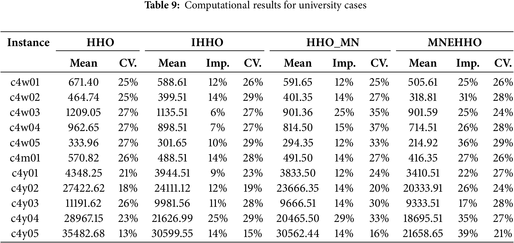
Finally, we report the results for university cases under low-reliability requirements (LPSP = 0.6) in Table 9. The findings indicate that HHO_MN reduces the objective value by an average of 31.4% compared to HHO for managing university-specific energy demands, particularly when relaxed reliability constraints permit more flexible optimization. This advantage is clearly illustrated in case c4w02, where MNEHHO achieves a mean objective value of 318.81, significantly outperforming other algorithms. The superiority of MNEHHO becomes even more evident during extended planning periods, as demonstrated in case c4y03, where its mean value of 9333.51 is considerably lower than those of HHO (11191.62), IHHO (9981.56), and HHO_MN (9666.51). This highlights MNEHHO’s capability to reduce the objective value by 16.6% in long-term university energy allocation under low-reliability requirements.

Analyzing the stability metrics reveals distinct patterns across the algorithms. The HHO algorithm exhibits moderate variability, with coefficient of variation (CV) values ranging from 13% to 27%, averaging 23%. In contrast, the IHHO algorithm demonstrates improved consistency, with CV values between 6% and 25%, averaging 12%. The HHO_MN algorithm maintains similar stability, with CV values ranging from 13% to 29%, averaging 22%. Meanwhile, the MNEHHO algorithm shows comparable stability, with CV values from 17% to 39%, averaging 27%. This indicates reliable performance across various university operational scenarios despite the more relaxed LPSP requirements.

The algorithmic improvements demonstrate significant performance enhancements across various test cases. This is particularly evident in c4y05, where HHO_MN achieves a 14% improvement over the HHO algorithm, while MNEHHO exhibits a 39% enhancement. These results highlight the effectiveness of combining improved HHO mechanisms with multiple neighborhood strategies for extended planning periods in university environments, particularly under lower reliability constraints.

Cross-case analysis demonstrates that MNEHHO’s performance advantages can be quantified across different application scenarios. In factory cases, where energy demands are highest, MNEHHO achieves improvements of up to 46%, with a mean improvement of 31.2% (σ = 8.4%) compared to the baseline HHO. For hospital cases that require high reliability, the algorithm demonstrates improvements of up to 40%, maintaining a mean improvement of 28.7% (σ = 7.2%). In hotel scenarios characterized by variable daily demands, MNEHHO produces improvements of up to 36%, with a mean of 27.9% (σ = 6.1%). Similarly, in university cases with lower reliability requirements, the algorithm achieves improvements of up to 39%, maintaining a mean improvement of 26.8% (σ = 7.8%). These consistent improvement patterns, supported by low standard deviations across all case types, demonstrate MNEHHO’s ability to optimize HRES allocations across diverse institutional settings with varying operational requirements.

Beyond these algorithmic improvements, the real value of our approach lies in its practical implications for facility-specific HRES implementation. The optimization results provide clear guidelines for system sizing, technology selection, and economic planning across different facility types, enabling more effective and efficient renewable energy deployments in real-world settings.

5  Conclusions

This study has addressed critical gaps in the optimal allocation of Hybrid Renewable Energy Systems (HRES) by developing a comprehensive mathematical model and an enhanced metaheuristic solution approach. Our key contributions can be summarized in three main aspects:

First, we have formulated a mathematical programming model that simultaneously considers multiple practical constraints that have been previously overlooked in the literature, including battery quantity calculations, charge-discharge efficiency, system reliability, and the fraction of renewable energy. This model offers a more accurate representation of the challenges associated with deploying HRES in real-world scenarios. Second, we have developed an enhanced version of the Harris Hawks Optimization algorithm that incorporates multiple neighborhood structures (MNEHHO). Our computational experiments demonstrate that MNEHHO consistently outperforms existing methods across various power demands. Specifically, it achieves improvements of up to 46% for factory cases, 40% for hospital cases, 36% for hotel cases, and 39% for university cases when compared to the HHO algorithm. The multiple neighborhood strategy proves particularly effective in handling larger, more complex instances while maintaining computational stability. Third, we have designed and implemented comprehensive test cases that represent four distinct real-world scenarios with varying reliability requirements and operational patterns. Our analysis provides insights into how these different institutional contexts influence optimal HRES configurations:

For future research directions, we propose several promising directions. Extending the model to incorporate weather uncertainty and demand variability will enhance its robustness for real-world applications. Future research should extend beyond algorithmic improvements to generate practical design insights and policy implications through incorporation of more comprehensive real-world data, socio-economic factors, and regulatory considerations. The mathematical framework and algorithmic approach developed in this study can serve as a foundation for broader HRES applications beyond institutional settings, including natural reserves and residential power systems. Our multi-neighborhood approach demonstrates particular adaptability to contexts with varying operational patterns and reliability requirements. Additionally, developing supplementary neighborhood structures could further improve solution quality, especially for long-term planning horizons. Investigating the potential integration of machine learning techniques to dynamically adjust algorithm parameters based on instance characteristics presents another valuable direction. The insights gained from institutional optimization can inform and accelerate HRES implementation across diverse contexts, ultimately supporting the global transition toward sustainable and resilient energy systems.

Acknowledgement: The author would like to thank anonymous reviewers, Associate Editor, and Editor-in-Chief for their constructive comments on earlier versions of the manuscript.

Funding Statement: The author received no specific funding for this study.

Availability of Data and Materials: The data used to support the findings of this study are included within the article.

Ethics Approval: Not applicable.

Conflicts of Interest: The author declares no conflicts of interest to report regarding the present study.

References

1. Adelekan OA, Ilugbusi BS, Adisa O, Obi OC, Awonuga KF, Asuzu OF, et al. Energy transition policies: a global review of shifts towards renewable sources [Internet]. Eng Sci Technol J. 2024 [cited 2025 Jan 1];5(2):272–87. Available from: https://api.semanticscholar.org/CorpusID:267602130. [Google Scholar]

2. Rao MVKS, Nguyen Ha Trang R. Sustainable and renewable energy initiatives across the globe: opportunities and challenges [Internet]. J Manage Res Anal. 2024 [cited 2025 Jan 1];11(1):18–23. Available from: https://api.semanticscholar.org/CorpusID:268312928. [Google Scholar]

3. As’ad S. Why renewable energy gained attention and demand globally? [Internet]. Nat Environ Pollut Technol, 2024;23:467–73. [cited 2025 Jan 1]. Available from: https://api.semanticscholar.org/CorpusID:268233821. doi:10.46488/NEPT.2024.v23i01.042. [Google Scholar] [CrossRef]

4. Das R, Bhattacharjee S, Das U. Importance of hybrid energy system in reducing greenhouse emissions. In: Kumar S, Gupta N, Kumar S, Upadhyay S, editors. Renewable energy systems: modeling, optimization and applications. Hoboken, NJ, USA: John Wiley & Sons, Inc.; 2022. [Google Scholar]

5. Pop CB, Cioara T, Anghel I, Antal M, Chifu VR, Antal C, et al. Review of bio-inspired optimization applications in renewable-powered smart grids: emerging population-based metaheuristics. Energy Rep. 2022;8:11769–98. doi:10.1016/j.egyr.2022.09.025. [Google Scholar] [CrossRef]

6. Agajie TF, Ali A, Fopah-Lele A, Amoussou I, Khan B, Velasco CLR, et al. A comprehensive review on tech-no-economic analysis and optimal sizing of hybrid renewable energy sources with energy storage systems. Energies. 2023;16(2):642. doi:10.3390/en16020642. [Google Scholar] [CrossRef]

7. Nassef AM, Abdelkareem MA, Maghrabie HM, Baroutaji A. Review of metaheuristic optimization algorithms for power systems problems. Sustainability. 2023;15(12):9434. doi:10.3390/su15129434. [Google Scholar] [CrossRef]

8. Corkish R, Lowe R, Largent R, Honsberg C, Shaw N, Constable R, et al. Montague Island Photovoltaic/Diesel Hy-brid system. In: Sixteenth European Photovoltaic Solar Energy Conference; 2020 May 1–5; Glasgow, Scotland. p. 2669–72. [Google Scholar]

9. Sowa S. The implementation of renewable energy systems, as a way to improve energy efficiency in residential buildings. Polityka Energetyczna. 2020;23(2):19–35. doi:10.33223/epj/122354. [Google Scholar] [CrossRef]

10. Haghighi BY, Mohamadian F, Ahmadi MH, Akbarianrad N. Medical and dental applications of renewable energy systems. Int J Low Carbon Technol. 2018;13(4):320–6. doi:10.1093/ijlct/cty040. [Google Scholar] [CrossRef]

11. Nirmal S, Rizvi T. A review of renewable energy systems for industrial applications. Int J Res Appl Sci Eng Technol. 2022;10(9):1740–5. doi:10.22214/ijraset.2022.46903. [Google Scholar] [CrossRef]

12. Trihardani L, Wang CT, Hsieh YJ. Making optimal location-sizing decisions for deploying hybrid renewable energy at B&Bs. Appl Sci. 2022;12(12):6087. doi:10.3390/app12126087. [Google Scholar] [CrossRef]

13. Al-Najjar H, Pfeifer C, Al Afif R, El-Khozondar HJ. Performance evaluation of a hybrid grid-connected photovol-taic biogas-generator power system. Energies. 2022;15(9):3151. doi:10.3390/en15093151. [Google Scholar] [CrossRef]

14. Jani HK, Kachhwaha SS, Nagababu G, Das A, Ehyaei M. Energy, exergy, economic, environmental, advanced ex-ergy and exergoeconomic (extended exergy) analysis of hybrid wind-solar power plant. Energy Environ. 2023;34(7):2668–704. doi:10.1177/0958305X221115095. [Google Scholar] [CrossRef]

15. Elattar EE, ElSayed SK. Probabilistic energy management with emission of renewable micro-grids including stor-age devices based on efficient salp swarm algorithm. Renew Energy. 2020;153:23–35. doi:10.1016/j.renene.2020.01.144. [Google Scholar] [CrossRef]

16. Kharrich M, Mohammed OH, Kamel S, Selim A, Sultan HM, Akherraz M, et al. Development and implementa-tion of a novel optimization algorithm for reliable and economic grid-independent hybrid power system. Appl Sci. 2020;10(18):6604. doi:10.3390/app10186604. [Google Scholar] [CrossRef]

17. Soheyli S, Mayam MHS, Mehrjoo M. Modeling a novel CCHP system including solar and wind renewable energy resources and sizing by a CC-MOPSO algorithm. Appl Energy. 2016;184:375–95. doi:10.1016/j.apenergy.2016.09.110. [Google Scholar] [CrossRef]

18. Li LL, Shen Q, Tseng ML, Luo S. Power system hybrid dynamic economic emission dispatch with wind energy based on improved sailfish algorithm. J Clean Prod. 2021;316:128318. doi:10.1016/j.jclepro.2021.128318. [Google Scholar] [CrossRef]

19. Çetinbaş İ, Tamyürek B, Demirtaş M. Sizing optimization and design of an autonomous AC microgrid for com-mercial loads using Harris Hawks optimization algorithm. Energy Convers Manage. 2021;245:114562. doi:10.1016/j.enconman.2021.114562. [Google Scholar] [CrossRef]

20. Gupta J, Nijhawan P, Ganguli S. Optimal sizing of different configuration of photovoltaic, fuel cell, and bio-mass-based hybrid energy system. Environ Sci Pollut Res. 2022;29(12):17425–40. doi:10.1007/s11356-021-17080-7. [Google Scholar] [PubMed] [CrossRef]

21. Rekioua D. Energy storage systems for photovoltaic and wind systems: a review. Energies. 2023;16(9):3893. doi:10.3390/en16093893. [Google Scholar] [CrossRef]

22. Niknam T, Golestaneh F, Malekpour A. Probabilistic energy and operation management of a microgrid containing wind/photovoltaic/fuel cell generation and energy storage devices based on point estimate method and self-adaptive gravitational search algorithm. Energy. 2012;43(1):427–37. doi:10.1016/j.energy.2012.03.064. [Google Scholar] [CrossRef]

23. Shin Y, Koo WY, Kim TH, Jung S, Kim H. Capacity design and operation planning of a hybrid PV-wind–battery-diesel power generation system in the case of Deokjeok Island. Appl Therm Eng. 2015;89:514–25. doi:10.1016/j.applthermaleng.2015.06.043. [Google Scholar] [CrossRef]

24. Ramli MA, Bouchekara H, Alghamdi AS. Optimal sizing of PV/wind/diesel hybrid microgrid system using mul-ti-objective self-adaptive differential evolution algorithm. Renew Energy. 2018;121:400–11. doi:10.1016/j.renene.2018.01.058. [Google Scholar] [CrossRef]

25. Nethercote N, Stuckey PJ, Becket R, Brand S, Duck GJ, Tack G. MiniZinc: towards a standard CP modelling lan-guage. In: International Conference on Principles and Practice of Constraint Programming; 2007 Sep 23–27; Providence, RI, USA. p. 529–43. [Google Scholar]

26. Thirunavukkarasu M, Sawle Y, Lala H. A comprehensive review on optimization of hybrid renewable energy sys-tems using various optimization techniques. Renew Sustain Energy Rev. 2023;176:113192. doi:10.1016/j.rser.2023.113192. [Google Scholar] [CrossRef]

27. Gezici H, Livatyali H. An improved Harris Hawks optimization algorithm for continuous and discrete optimization problems. Eng Appl Artif Intell. 2022;113:104952. doi:10.1016/j.engappai.2022.104952. [Google Scholar] [CrossRef]