1 Introduction
This part consists of two subsections. In the first section relevant literature is presented while the second part is about the motivation and research gap.
1.1 Literature Review
The real world is full of complex issues. Engineering, social science, management science, and economics are a few of the major real-world fields. Imprecision, vagueness, and uncertainty are the main issues we are dealing with in the aforementioned fields. These problems have a variety of uncertainties, which makes it impossible for us to solve them using traditional methods. The interval mathematics theory, theory of probability, fuzzy set theory, and rough sets theory are just a few of the numerous theories. To improve uncertainty modeling and provide more flexibility, Saeed et al. [1] provide refined fuzzy soft sets that offer a comprehensive approach to analyzing data while addressing the challenges of uncertainty and ambiguity in real-world data. A better representation of ambiguous and parameter-dependent data is possible with this hybrid approach, which combines the best features of both techniques. The concept of the fuzzy soft set was applied to the decision-making problems by different researchers (see, e.g., references [2–4] and the cited works within). To improve decision-making in situations when there is uncertainty among several membership values, Ali et al. [5] expanded the hesitant fuzzy soft set architecture. This method provides a deeper understanding of uncertainty, which offers a full range of information measures for hesitant fuzzy soft sets. It is more adaptable than earlier models and may be used for intricate and unpredictable problems. It develops decision-making scenarios by offering a more precise and flexible framework for dealing with these difficulties. Similarly, fuzzy and hesitant fuzzy concepts [6] manipulate data uncertainty modeling in a descent manner as well as a powerful tool for solving multi-criteria decision-making challenges raised in machine learning problems [7]. Recent developments in fuzzy and hesitant fuzzy sets have greatly enhanced frameworks for making decisions. For instance, an improved hesitant fuzzy model for multi-criteria decision-making was presented by Shen et al. [8]. More recently, Ali et al. [9] suggested a hybrid approach for election prediction scenarios that combine soft expert sets with dual hesitant fuzzy sets. Nevertheless, in spite of these developments, Suzuki-type (μ,ν)-weak contractions have not yet been integrated with hesitant fuzzy soft set-valued mappings, especially for scenarios with substantial ambiguity and hesitation. The purpose of this study is to close this gap.
Now, such scenarios can be manipulated more appropriately by the representation of mappings. So researchers are trying to model real-world complex issues using multi-valued mappings. So for this purpose, fuzzy and soft set valued mappings are employed to manage and arrive at decisions in scenarios including ambiguity, imprecision, or uncertainty. The main aim of the soft set-valued map is to assign items to sets rather than single values to address data uncertainty. Similarly fuzzy soft set valued mappings are used for managing even more complicated uncertainty. So, a family of fuzzy mapping that takes a broad view of the idea of set-valued mappings was introduced in 1981 by Heilpern [10] using the concept of fuzzy sets. During this procedure, he revealed the presence of the fuzzy fixed point theorem, advancing over Nadler’s fixed point theorem [11] and the Banach contraction theorem [12] for multi-valued mapping. Frigon et al. [13] enhanced the Heilpern fixed point theorem for the case in which it should be under observation that 1-level sets are not supposed to be compact and convex beneath a contractive reservation. Later, on metric and quasi-metric spaces, several researchers investigated the presence of fixed and joint fixed points of fuzzy mapping sustaining different kinds of contractive constraints (see, e.g., references [14–17] and the cited works within).
1.2 Motivation
Existing fuzzy set frameworks are inadequate for solving many decision-making problems that involve hesitation and ambiguity. Though their potential in conjunction with sophisticated contraction principles is still unexplored, hesitant fuzzy soft sets provide a novel method for modeling such issues. Finding fixed-point outcomes for hesitant fuzzy soft set-valued mappings using Suzuki-type (μ,ν)-weak contractions is the goal of this work. The goals are to produce theoretical results, show how they might be used, and compare them to current approaches. Suzuki-type weak contractions characterize metric completeness and generalize the Banach contractions [18]. Suzuki-type contractions can handle multi-valued mapping problems adequately [19–21]. For this reason, Suzuki-type weak contraction is chosen for this study. Because it considers the inherent uncertainties and hesitation in real-world data, the Suzuki-type (μ,ν)-weak contraction is especially well-suited for hesitant fuzzy soft set-valued mappings. Through its parameters μ and ν, it provides more flexibility than classical contraction principles, allowing for more precise control over the mapping process. This guarantees convergence to fixed points under more general circumstances and enables a more accurate depiction of intricate interactions. It is the perfect option for applications needing sophisticated decision-making frameworks because of these features [22]. Because it considers the two problems of uncertainty and hesitation that arise in real-world decision-making, the Suzuki-type (μ,ν)-weak contraction is especially well-suited for hesitant fuzzy soft set-valued mappings. The dual-parameter structure of Suzuki-type contractions provides for more precise control over mapping behavior than standard fuzzy set generalizations, which might not be able to capture multi-valued dependencies. Because of this, it is perfect for resolving difficult decision-making issues where conventional approaches are inadequate.
1.3 Research Gaps
The integration of hesitant fuzzy soft sets with sophisticated fixed-point theorems, such as Suzuki-type (μ,ν)-Weak Contractions, has not been discovered, even though they have been thoroughly examined in the context of uncertainty modeling. Current approaches, such as classical contraction principles, can not ensure convergence under more general circumstances and have limitations when dealing with multi-valued membership structures. Furthermore, although hesitant fuzzy sets have a wealth of research on their usage in decision-making, nothing is known about how they might be used with dual-parameter contraction techniques to address practical issues. By creating a thorough framework for hesitant fuzzy soft set-valued mappings and showing its usefulness in real-world scenarios, this work seeks to close these gaps. So, in this work, we study fixed point via Suzuki-type (μ,ν)-weak contraction under a new framework of study which is a hesitant fuzzy soft set-valued mapping. We extend the concept of Suzuki-type (μ,ν)-weak contraction in the context of hesitant fuzzy soft set-valued mapping and explore sufficient conditions for establishing a hesitant fuzzy soft fixed point for the mentioned contractions, inspired by the work of Shagari et al. [23]. In addition to expanding the scope of contraction principles, the suggested method tackles real-world decision-making difficulties, which advances fuzzy mathematics and its purposes. The established work generalizes the related notions of fuzzy sets, soft sets, and multi-valued maps within the framework of metric spaces. Furthermore, a decision-making problem is also addressed using the presented results. With, the help of a hesitant fuzzy soft fixed point we find out an optimal result in the example.
1.4 Proposed Decision-Making Application
A real-world decision-making problem involving multi-criteria group decision-making under uncertainty is used in this study to test the suggested framework. Hesitancy and competing preferences are considered when modeling the situation using hesitant fuzzy soft set-valued mappings. Suzuki-type (μ,ν)-weak contractions permit dual-parameter control, which allows for iterative solution refining and optimal decision-making. This method can be used, for instance, to choose the best option from a range of selections or allocate resources while considering preference hesitancy.
1.5 Overview of the Methodology
Following the definition of hesitant fuzzy soft set-valued mappings, Suzuki-type (μ,ν)-weak contraction principles are applied to construct fixed-point outcomes and conclude the approach. The hesitant fuzzy values are refined by an iterative process that guarantees convergence to a fixed point representing the best course of action. In order to validate the theoretical results and show how resilient the approach is, numerical examples and a real-world application are given. This research manuscript is split into four parts. In the first part, literature review and motivation are given, the second section consists of necessary definitions, the third section consists of our main work, and in the fourth section, applications of the presented results are discussed.
2 Preliminaries
In this part of the paper, we need some results and definitions from the existing literature. Throughout this manuscript, we represent a metric function by “D”, W be a non-empty set and the set of all hesitant fuzzy soft sets by H~(W)E.
Definition 1. [23] Let W be a non-empty set. A mapping Lˇ: W⟶W is known as weak contraction if ∃, a constant ζ∈(0,1) and K≥0 such that
D(Lˇw,Lˇb)≤ζD(w,b)+KD(b,Lˇw);∀,b,w∈W.
Definition 2. [23] Assume that (W, D) be a metric space and Lˇ: W⟶ CB(W) is a multi-valued mapping. Then Lˇ is known as multi-valued weak contraction or multi-valued (ϑ, K)-weak contraction iff ∃, constants ϑ ∈ (0, 1) and K ≥ 0 such that
H(Lˇw,Lˇb)≤ϑD(w,b)+KD(b,Lˇw);∀,w,b∈W.
Definition 3. [22] A couple (G, E) be known as a soft set on (W) iff G is a function from E into the P(W).
Definition 4. [5] Assume that a hesitant fuzzy set B on W be in the form of a mapping over W, gives us a subset of [0, 1], and mathematically be determined by
B={⟨w,hB~(w)⟩∣w∈W}.
In the above set, hB~(w) represents the possible values of membership degrees in [0, 1] of ‘w’ ∈W to B. For simplicity, hB~(w) is called a hesitant fuzzy element. So, all hesitant fuzzy elements are represented by a set H.
Definition 5. [23] Assume that ℏ is a hesitant fuzzy element in B. Then its score function is determined by
Sc(ℏ)=(1N(ℏ))∑ς∈ℏς.
So, N(ℏ) shows number of objects in ℏ and actually Sc(ℏ) represents the average of the objects in ℏ and Sc(ℏ) ∈[0,1].
Definition 6. [23] Given that μ∈(0,1], then ordinary crisp subset of W determined as
ℏμA={t∈W:Sc(ℏA(t))≥μ},
be known as μ-cut of the hesitant fuzzy soft A on W.
Definition 7. [5] Suppose H~(W) is the power set of hesitant fuzzy set in W; a pair (G~,A) is said to be a hesitant fuzzy soft set over W, where G~ is a mapping given by G~:A→H~(W).
3 Hesitant Fuzzy Soft Fixed Points of Suzuki-Type (μ,ν)-Weak Contraction
In this part of our manuscript we present some definitions and the main results. Now motivated by the Definition 6 we can defined μ-cut of the hesitant fuzzy soft set (G~,A) as follows:
Definition 8. Given μ ∈ (0, 1] then the ordinary subset means crisp subset of W can be presented by
ℏμG~e={w∈W:Sc(hG~e(w))≥μ},
is known as the μ-cut of the hesitant fuzzy soft set G~ on W.
Definition 9. The mapping Lˇ:W→ H~(W)E is called hesitant fuzzy soft set valued mapping.
Remark 1. The above definition is the extended version of the hesitant fuzzy set-valued mapping of the paper [22]. Where, note that if Lˇ is a hesitant fuzzy soft set valued mapping on W, then Lˇw: E → H~(W) is a hesitant fuzzy soft set, i.e., for each w ∈W and (Lˇw)(ë) = Lˇ(w;e)∈ H~(W) is a hesitant fuzzy soft, so for each w ∈ W, Lˇ(w;e)(w)⊆[0,1] is a hesitant fuzzy element (HFE).
Definition 10. Assume that Lˇ:W→ H~(W)E is a hesitant fuzzy soft set valued mapping, w ∈W, e ∈ Dom Lˇw and μ∈ (0, 1]. So, the μ-level set of Lˇ is represented by
[Lˇ(w;e)]μ={r∈W:S([Lˇ(w;e)](r)≥μ}.
Remark 2. Definition 10 is an extended form of μ-level set of hesitant fuzzy set valued mapping [22]. Here for w ∈W, Lˇw H~(W)E, that is, Lˇw:E⟶H~(W). This represents that (Lˇw)(e)=Lˇ(w;e)∈H~(W). This implies that Lˇ(w;e):W→P(I), hence Lˇ(w;e)(r) ⊆ I. So that for μ∈I, [Lˇ(w;e)]μ is well-given.
Here I = [0, 1], P(I) represents collection of all subsets of I = [0, 1].
Definition 11. A point w is said to be hesitant fuzzy soft-fixed point of Lˇ:W⟶H~(W)E, if ∃, e ∈ E and μ∈ (0, 1] for which w ∈[Lˇ(w;e)]μ. The point w is known as a common hesitant fuzzy soft-fixed point of Sˇ, Lˇ:W⟶H~(W)E if w ∈[Sˇ(w;e)]μ∩[Lˇ(w;e)]μ.
Remark 3. The Definition 11 is an enhanced form of hesitant fuzzy fixed point of the paper [22].
Definition 12. A mapping Lˇ:W→H~(W)E is said to be a hesitant fuzzy soft set valued mapping. A point w∈W is known as an e-hesitant fuzzy soft-fixed point of Lˇ if w∈[Lˇ(w;e)]μ, for some e∈E and μ∈(0,1]. It can be written as w∈[Lˇw]μ, for short. If Dom(Lˇw)=E, and w∈[Lˇ(u;e)]μ,∀,e∈E, then w is known as an E-hesitant fuzzy soft fixed point of Lˇ.
Here the set of all E-hesitant fuzzy soft fixed points of a hesitant fuzzy soft set valued mapping Lˇ is represented by E−HFSFix(Lˇ).
Definition 13. Assume that W≠⧸0 and E be set of parameters and Lˇ be a hesitant fuzzy soft set on W. Choosing (μ,ν)∈(0,1]×[0,1), the crisp subset of W determined by
(Lˇw;e)(μ,ν)={t∈W:Sc((Lˇw;e)(t))≥μ}∪{t∈W:Sc((Lˇw;e)(t))≤ν},
is known as the (μ,ν)-level set of Lˇ, and here Sc((Lˇw;e)(t)) shows score function of Lˇ. So, a point u^∈W is known hesitant fuzzy soft fixed point of Lˇ if ∃,(μ,ν)∈(0,1]×[0,1) such that u^∈(Lˇu^;e)(μ,ν).
Note that in the whole manuscript, the function r:(0,1)⟶(1/2,1] is defined by
r(μ)={1, if 0<μ<1/2,1−μ, if 1/2≤μ<1.(1)
For w,b∈W and (μ,ν)∈(0,1]×[0,1), defining
∨(w,b)=max{D(w,b),D(w,(Lˇw;e)(μ,ν)),D(b,(Lˇb;e)(μ,ν)),D(w,(Lˇb;e)(μ,ν))+D(b,(Lˇw;e)(μ,ν))2,D(w,(Lˇw;e)(μ,ν))D(b,(Lˇb;e)(μ,ν))1+D(w,b)},∧(w,b)=min{D(w,(Lˇw;e)(μ,ν)),D(b,(Lˇw;e)(μ,ν)),D(w,(Lˇw;e)(μ,ν))D(b,(Lˇb;e)(μ,ν))1+D(w,b)}.
Remark 4. Definition 13 generalizes the Definition [9] of the paper [23].
Definition 14. A hesitant fuzzy soft set valued mapping Lˇ:W⟶H~(W)E is known as Suzuki-type (μ,ν)-weak contraction if ∀,w,b∈W with w≠b and e∈A⊆E,∃, some (μ,ν)∈(0,1]×[0,1) such that
r(μ)D(w,[Lˇ(w;e)](μ,ν))≤D(w,b).
Then we have
H((Lˇw;e)(μ,ν),(Lˇb;e)(μ,ν))≤μ∨(w,b)+ν∧(w,b).
Theorem 1. Assume that (W,D) is a complete metric space and Lˇ:W⟶H~(W)E is a Suzuki-type (μ,ν)-weak contraction. Suppose that ∀,w∈W, and e∈A⊆E,∃,(μ,ν)∈(0,1]×[0,1) such that [Lˇ(w;e)](μ,ν)≠⧸0, closed and bounded subset of W. Then Fix(Lˇ)≠ϕ.
Proof. Assume that (μ,ν)∈(0,1]×[0,1) be such that 0<μ≤μ1<1,w1∈W and ρ=1/μ. Assume that (Lˇw1;e)(μ,ν)≠⧸0. So, we can find w2∈W such that w2∈(Lˇw1;e)(μ,ν). Since ρ>1, choose w3∈(Lˇw2;e)(μ,ν) such that
D(w2,w3)≤ρH((Lˇw1;e)(μ,ν),(Lˇw2;e)(μ,ν)).
If w1=w2, then w1∈(Lˇw1;e)(μ,ν) for some (μ,ν)∈(0,1]×[0,1) and hence theorem is proved. Suppose w1≠w2. Since r(μ)≤1, Further suppose that
r(μ)D(w1,(Lˇw1;e)(μ,ν))≤D(w1,(Lˇw1;e)(μ,ν))≤D(w1,w2)
Then we have
D(w2,w3)≤ρH((Lˇw1;e)(μ,ν),(Lˇw2;e)(μ,ν))≤1μ(μ∨(w,b)+ν∧(w,b))(2)
≤μmax{D(w1,w2),D(w1,(Lˇw1;e)(μ,ν)),D(w2,(Lˇw2;e)(μ,ν)),D(w1,(Lˇw2;e)(μ,ν))+D(w2,(Lˇw1;e)(μ,ν))2,D(w1,(Lˇw1;e)(μ,ν))D(w2,(Lˇw2;e)(μ,ν))1+D(w1,w1)+νμminD(w1,(Lˇw1;e)(μ,ν)),D(w2,(Lˇw1;e)(μ,ν)),D(w1,(Lˇw1)(μ,ν))D(w2,(Lˇw2)(μ,ν))1+D(w1,w2)}≤μmax{D(w1,w2),D(w2,w3),D(w1,w3)+D(w2,w2)2,D(w1,w2)D(w2,w3)1+D(w1,w2)}+νμmin{D(w1,w2),D(w2,w2),D(w1,w2)D(w2,w3)1+D(w1,w2)}≤μmax{D(w1,w2),D(w2,w3),D(w1,w2)+D(w2,w3)2}≤μmax{D(w1,w2),D(w2,w3)}(3)
If D(w1,w2)≤D(w2,w3), then from Eq. (3), we have
D(w2,w3)≤μD(w2,w3)<D(w2,w3),
a contradiction. Hence, D(w1,w2)>D(w2,w3) and Eq. (3) becomes
D(w2,w3)≤μD(w1,w2)≤μ1D(w1,w2).
To continue the above process, we can make a progression {wn}n∈N in W such that
wn+1∈(Lˇwn;e)(μ,ν)
and
D(wn,wn+1)≤μ1D(wn−1,wn).
So we obtain
∑n=1∞D(wn,wn+1)≤∑n=1∞(μ1)n−1D(w1,w2)<∞.
As a result, we came to know that {wn}n∈N be a Cauchy progression in W. So, completeness of W shows that ∃,u^∈W such that wn⟶u^ as n⟶∞. Assume: ∀,u^≠w, then we get
D(u^,(Lˇw;e)(μ,ν))≤μmax{D(u^,w),D(w,(Lˇw;e)(μ,ν))}(4)
Since wn⟶u^ as n⟶∞,∃, a natural number k such that
5D(wn,u^)≤D(u^,w)∀,n≥k.
We are given that wn+1∈(Lˇwn;e)(μ,ν), we obtain
r(μ)D(wn,(Lˇwn;e)(μ,ν))≤D(wn,(Lˇwn;e)(μ,ν))≤D(wn,wn+1)≤D(wn,u^)+D(u^,wn+1)≤25D(u^,w)
Hence, for n≥k, we obtain
r(μ)D(wn,(Lˇwn;e)(μ,ν))≤25D(u^,w)≤D(u^,w)−15D(u^,w)≤D(u^,w)−D(u^,wn)≤D(wn,w).(5)
Hence, applying Eq. (5) we get
D(wn+1,(Lˇw;e)(μ,ν))≤H((Lˇwn;e)(μ,ν),(Lˇw;e)(μ,ν))≤μmax{D(wn,w),D(wn,(Lˇwn;e)(μ,ν)),D(w,(Lˇw;e)(μ,ν)),D(wn,(Lˇw;e)(μ,ν))+D(w,(Lˇwn;e)(μ,ν))2,D(wn,(Lˇwn;e)(μ,ν))D(w,(Lˇw;e)(μ,ν))1+D(wn,w)}+ν min{D(wn,(Lˇwn;e)(μ,ν)),D(w,(Lˇwn;e)(μ,ν)),D(wn,(Lˇwn;e)(μ,ν))D(w,(Lˇw;e)(μ,ν))1+D(wn,w)}.(6)
From Eq. (6), we have
D(wn+1,(Lˇw;e)(μ,ν))≤μmax{D(wn,w),D(wn,wn+1),D(w,(Lˇw;e)(μ,ν)),D(wn,(Lˇw;e)(μ,ν))+D(w,wn+1)2,D(wn,(Lˇwn;e)(μ,ν))D(w,(Lˇw;e)(μ,ν))1+D(wn,w)}+νmin{D(wn,wn+1),D(w,wn+1),D(wn,wn+1)D(w,(Lˇw;e)(μ,ν))1+D(wn,w).}.(7)
Since we know that in (7) as n⟶∞, so we get
D(u^,(Lˇw;e)(μ,ν))≤μmax{D(u^,w),D(w,(Lˇw;e)(μ,ν)),D(u^,(Lˇw;e)(μ,ν))+D(u^,w)2}+νmin{0,D(u^,w)}≤μmax{D(u^,w),D(w,(Lˇw;e)(μ,ν))}.
Next we will show that u^∈(Lˇu^;e)(μ,ν), for this we assume the following two cases.
Case (1). 0 < μ < 1/2.
Assume that ∀,(μ,ν)∈(0,1]×[0,1) with μ<1,u^≠p,u^∉(Lˇu^;e)(μ,ν) and p∈(Lˇu^;e)(μ,ν) such that
D(p,u^)<D(u^,(Lˇu^;e)(μ,ν)).
Setting w=p in Eq. (4), we have
D(u^,(Lˇp;e)(μ,ν))≤μmax{D(u^,p),D(p,(Lˇp;e)(μ,ν))}(8)
Now,
r(μ)D(u^,(Lˇu^;e)(μ,ν))≤D(u^,(Lˇu^;e)(μ,ν))≤D(u^,p).
Then we have
D(p,(Lˇp;e)(μ,ν))≤H((Lˇu^;e)(μ,ν),(Lˇp;e)(μ,ν))≤μmax{D(u^,p),D(u^,(Lˇu^;e)(μ,ν)),D(p,(Lˇp;e)(μ,ν)),D(u^,(Lˇp;e)(μ,ν))+D(p,(Lˇu^;e)(μ,ν))2,D(u^,(Lˇu^;e)(μ,ν))D(p,(Lˇp;e)(μ,ν))1+D(u^,p)}+νmin{D(u^,(Lˇu^;e)(μ,ν)),D(p,(Lˇu^;e)(μ,ν)),D(u^,(Lˇu^;e)(μ,ν))D(p,(Lˇp;e)(μ,ν))1+D(u^,p)}.≤μmax{D(u^,p),D(p,(Lˇp;e)(μ,ν)),D(u^,(Lˇp;e)(μ,ν))2,D(u^,p)D(p,(Lˇp;e)(μ,ν))1+D(u^,p)}+νmin{D(u^,p),0,D(u^,p)D(p,(Lˇp;e)(μ,ν))1+D(u^,p)}≤max{D(u^,p),D(p,(Lˇp;e)(μ,ν)),D(u^,p)+D(p,(Lˇp;e)(μ,ν))2}≤μmax{D(u^,p),D(p,(Lˇp;e)(μ,ν))}.
Suppose that D(u^,p)≤D(p,(Lˇp;e)(μ,ν)), so we get from the above inequalities as below:
D(p,(Lˇp;e)(μ,ν))≤μD(p,(Lˇp;e)(μ,ν))<D(p,(Lˇp;e)(μ,ν)),
which shows a contradiction. So,
D(u^,p)>D(p,(Lˇp;e)(μ,ν)),
and
D(p,(Lˇp;e)(μ,ν))≤μD(u^,p)<D(u^,p).
So Eq. (8) will be
D(u^,(Lˇp;e)(μ,ν))≤μD(u^,p).
Consequently,
D(u^,(Lˇu^;e)(μ,ν))≤D(u^,(Lˇp;e)(μ,ν))+H((Lˇp;e)(μ,ν),(Lˇu^;e)(μ,ν))≤D(u^,(Lˇp;e)(μ,ν))+μmax{D(u^,p),D(p,(Lˇp;e)(μ,ν))}≤μD(u^,p)+μD(u^,p)=2μD(u^,p)<D(u^,p)<D(u^,(Lˇu^;e)(μ,ν)).
So, our supposition gives a contradiction. Therefore, u^∈(Lˇu^;e)(μ,ν). Case (2). 1/2 ≤ μ < 1. Now, we will prove that
H((Lˇw;e)(μ,ν),(Lˇu^;e)(μ,ν))≤μmax{D(,w),D(w,(Lˇw;e)(μ,ν)),D(u^,(Lˇu^;e)(μ,ν)),D(w,(Lˇu^;e)(μ,ν))+D(u^,(Lˇw;e)(μ,ν))2,D(w,(Lˇw;e)(μ,ν))D(u^,(Lˇu^;e)(μ,ν))1+D(u^,w)}+νmin{D(w,(Lˇw;e)(μ,ν)),D(u^,(Lˇw;e)(μ,ν)),D(u^,(Lˇu^;e)(μ,ν))D(w,(Lˇw;e)(μ,ν))1+D(u^,w)}.(9)
satisfied ∀,w∈W with w≠u^. Now, ∀,m∈N,∃,vm∈(Lˇw;e)(μ,ν) such that
D(u^,vm)≤D(u^,(Lˇw;e)(μ,ν))+15mD(u^,w).
Thus, we have
D(w,(Lˇw;e)(μ,ν))≤D(w,vm)≤D(w,u^)+D(u^,vm)≤D(w,u^)+D(u^,(Lˇw;e)(μ,ν))+15mD(w,u^).
Using Eq. (4), we have
D(w,(Lˇw;e)(μ,ν))≤D(u^,w)+μmax{D(u^,w),D(w,(Lˇw;e)(μ,ν))}+15m.(10)
If D(w,u^)>D(w,(Lˇw;e)(μ,ν)), then from Eq. (10), we get
D(w,(Lˇw;e)(μ,ν))≤D(u^,w)+μD(u^,w)+15mD(u^,w)=[(1+μ)+15m]D(u^,w).
from which we have
[11+μ]D(w,(Lˇw;e)(μ,ν))≤[1+15(1+μ)m]D(u^,w).
Using r(μ) = 1 − μ, we get
r(μ)D(w,(Lˇw;e)(μ,ν))=(1−μ)D(w,(Lˇw;e)(μ,ν))≤(11+μ)D(w,(Lˇw;e)(μ,ν))≤[1+15(1+μ)m]D(u^,w)
From the above inequalities as m⟶∞, we get
r(μ)D(w,(Lˇw;e)(μ,ν))≤D(u^,w).
From the other side, if
D(u^,w)<D(w,(Lˇw;e)(μ,ν)),
then Eq. (10) gives
D(w,(Lˇw;e)(μ,ν))≤D(u^,w)+μD(w,(Lˇw;e)(μ,ν))+15mD(u^,w)
Which yields
(1−μ)D(w,(Lˇw;e)(μ,ν))≤(1+15m)D(u^,w).
So, in the above inequality when m⟶∞, we get
(1−μ)D(w,(Lˇw;e)(μ,ν))≤D(u^,w).
It means that
r(μ)D(w,(Lˇw;e)(μ,ν))≤D(u^,w).
Which is an output of the Definitions 13 and 14 collectively. Furthermore, since
wn+1≠wn∀,n∈N,thenu^≠wn+1.
Therefore, keeping wn = w in Eq. (9), we obtain
D(wn+1,(Lˇu^;e)(μ,ν))≤H((Lˇwn;e)(μ,ν),(Lˇu^;e)(μ,ν))≤μmax{D(wn,u^),D(wn,(Lˇwn;e)(μ,ν)),D(u^,(Lˇu^;e)(μ,ν)),D(wn,(Lˇu^;e)(μ,ν))+D(u^,(Lˇwn;e)(μ,ν))2,D(wn,(Lˇwn;e)(μ,ν))D(u^,(Lˇu^;e)(μ,ν))1+D(wn,u^)}+kmin{D(wn,(Lˇwn;e)(μ,ν)),D(u^,(Lˇwn;e)(μ,ν)),D(wn,(Lˇwn;e)(μ,ν))D(u^,(Lˇu^;e)(μ,ν))1+D(wn,u^)}≤μmax{(D(wn,u^),D(wn,wn+1),D(u^,(Lˇu^;e)(μ,ν)),D(wn,(Lˇu^;e)(μ,ν))+D(u^,wn+1)2,D(wn,wn+1)D(u^,(Lˇu^;e)(μ,ν))1+D(wn,u^)}+νmin{D(wn,wn+1),D(u^,wn+1),D(wn,wn+1)D(u^,(Lˇu^;e)(μ,ν))1+D(wn,u^)}
In the above inequalities as n⟶∞, we get
D(u^,(Lˇu^;e)(μ,ν))≤μmax{D(u^,(Lˇu^;e)(μ,ν)),D(u^,(Lˇu^;e)(μ,ν))2,0}≤μD(u^,(Lˇu^;e)(μ,ν)).(11)
Since 1 − μ> 0, therefore, using Eq. (11), we get
D(u^,(Lˇu^;e)(μ,ν))=0,
and as a result, u^∈(Lˇu^;e)(μ,ν).□
Corollary 1. Assume that (W, D) be a complete metric space and Lˇ:W→H(W)E be a hesitant fuzzy soft mapping. Assume that for w,b∈W with w≠b,∃,(μ,ν)∈(0,1]×[0,1) such that (Lˇw;e)(μ,ν)≠⧸0, bounded and closed subset of W. If r(μ)D(w,(Lˇw;e)(μ,ν))≤D(w,b) implies H((Lˇw;e)(μ,ν),(Lˇb;e)(μ,ν))≤μ∨(w,b), then Fix(Lˇ)≠ϕ.
Further, we provide a local hesitant fuzzy fixed point theorem for Suzuki-type (μ,ν)−WC. First of all, we remember the definition of the open ball having radius r^> 0, centered at w0 in a metric space W, is represented by
Br^(w0)={w∈W:D(w,w0)<r^}.
Theorem 2. Assume that (W, D) be a complete metric space, Lˇ:Br^(w0)⟶H(W)E be a Suzuki-type (μ,ν)-WC. Suppose that ∀,w∈W,∃,(μ,ν)∈(0,1]×[0,1) such that (Lˇw;e)(μ,ν)≠ϕ, closed and bounded subset of W, and D(w0,(Lˇw0;e)(μ,ν))<(1−μ)r^. Then Fix(Lˇ)≠ϕ.
Proof. Assume that 0<γ<r^ is chosen in such a way that
0<(1−μ)(1+μ)≤1/(1+γ),Bγ∗(w0)⊂Br(w0)andD(w0,(Lˇw0;e)(μ,ν))<(1−μ)γ.
Therefore,
(1−μ)γ−D(w0,(Lˇw0;e)(μ,ν))>0.
Choose γ=(1−μ)γ−D(w0,(Lˇw0;e)(μ,ν))>0; then ∃,w1∈(Lˇw0;e)(μ,ν) such that
D(w0,w1)<D(w0,(Lˇw0;e)(μ,ν))+γ.
Thus, D(w0,w1)<(1−μ)γ. Now, for ρμ=1 and
w1∈(Lˇw0;e)(μ,ν),∃,w2∈(Lˇw1;e)(μ,ν)
such that
D(w1,w2)≤ρH((Lˇw0;e)(μ,ν),(Lˇw1;e)(μ,ν)).
Noting that r(μ)D(w0,(Lˇw0;e)(μ,ν))≤r(μ)D(w0,w1)≤D(w0,w1).
We have
D(w1,w2)≤ρH((Lˇw0;e)(μ,ν),(Lˇw1;e)(μ,ν))=1μH((Lˇw0;e)(μ,ν),(Lˇw1;e)(μ,ν))≤μ∨(w0,w1)+νμ∧(w0,w1)≤μmax{D(w0,w1),D(w0,(Lˇw0;e)(μ,ν)),D(w1,(Lˇw1;e)(μ,ν)),D(w0,(Lˇw1;e)(μ,ν))+D(w1,(Lˇw0;e)(μ,ν))2,D(w0,(Lˇw0;e)(μ,ν))D(w1,(Lˇw1;e)(μ,ν))1+D(w0,w1)}+νμmin{D(w0,(Lˇw0;e)(μ,ν)),D(w1,(Lˇw0;e)(μ,ν)),D(w0,(Lˇw0;e)(μ,ν))D(w1,(Lˇw1;e)(μ,ν))1+D(w0,w1)}≤μmax{D(w0,w1),D(w0,w1),D(w1,w2),D(w0,w2)+D(w1,w1)2,D(w0,w1)D(w1,w2)1+D(w0,w1)}+νμmin{D(w0,w1),D(w1,w1),D(w0,w1)D(w1,w2)1+D(w0,w2)}≤μmax{D(w0,w1),D(w1,w2),D(w0,w1)+D(w1,w2)2}+νμmin{D(w0,w1),0,D(w1,w2)}≤μmax{D(w0,w1),D(w1,w2)}
If D(w0,w1)≤D(w1,w2), then the above gives
D(w1,w2)≤μD(w1,w2)<D(w1,w2),
a contradiction. Hence,
D(w0,w1)>D(w1,w2)
and
D(w1,w2)<μD(w0,w1)μ(1−μ)γ.
So by our supposition and the triangle inequality, we have
D(w0,w2)≤D(w0,w1)+D(w1,w2)<(1−μ)γ+μ(1−μ)γ≤γ1+γ<γ
Hence, w2∈Bγ(w0). So by recursive process we make a progression {wn}n∈N such that
1. wn∈Bγ(w0);∀,n∈N;
2. wn∈(Lˇwn;e)(μ,ν);∀,n∈N;
3. D(wn,wn+1)≤(μ)n(1−μ)γ;∀,n∈N.
From (3), it is clearly known that {wn}n∈N is a Cauchy progression and shrinks to some u^∈Br(w0). Furthermore, after this step, we can follow the steps of the Theorem 1, as a result, we get that
Fix(Lˇ)≠ϕ.◻
Corollary 2. Assume that (W,D) be a complete metric space and Λ:W⟶CB(W) be a multi-valued mapping. Suppose that ∀,w,b∈W,∃,(μ,ν)∈I+×[0,1) such that r(μ)D(w,Λw)≤D(w,b) implies H(Λw,Λb)≤μ∨(w,b)+ν∧(w,b), and the mapping r:(0,1)⟶I+1 is determined by
r(μ)={1,if0≤μ<1/21−μ,if1/2≤μ<1.(12)
Then Fix(Λ)≠ϕ.
Proof. Assume that I+=(0,1] and P(I+) be the power set of I+. Suppose we have a map Ψ:W⟶P(I+) and a hesitant fuzzy soft map Lˇ:W⟶H~(W)E defined by
(Lˇw;e)(t¨)={Ψ(w)∖{1},ift¨∈Λw,{1},ift¨∉Λw.(13)
Assume that, μ=inf{s((Lˇw;e)(t¨)):t¨∈W} and ν=0. Then,
(Lˇw;e)(μ,ν)={t¨∈W:s((Lˇw;e)(t¨))≥μ}∪{t¨∈W:Sc((Lˇw;e)(t¨))≤ν}=Λw.
Therefore,
D(w,b)≥r(μ)D(w,Λw)=r(μ)D(w,(Lˇw;e)(μ,ν)).
Hence, now we can use Theorem 1 to search out u^∈W such that u^∈Λu^. □
4 Applications
This part of our manuscript consists of examples: In the consequence of Theorem 1 the following example is provided.
Example 1. Assume that W={4,5,6},{4},{5},{6} be crisp sets and E={e1¨,e2¨} is the set of attributes. Define D:W×W⟶R as follows:
D(w,b)={0,ifw=b,7/20, if w≠b and w,b∈W ∖{5},1,if w≠b and w,b∈W ∖{6},9/20,if w≠b and w,b∈W ∖{4}.
Define a hesitant fuzzy soft mapping Lˇ:W⟶H~(W)E as follows:
(Lˇw;e1)t¨={{0.6,0.8,1},if t¨=4,{0.2,0.5,0.7},if t¨=5,{0,0.3,0.4}, if t¨=6,
(Lˇw;e2)t¨={{0.1,0.4,0.5}, if t¨=4,{0.3,0.6,0.8}, if t¨=5,{0.5,0.7,0.9},if t¨=6.
For w∈W and e1∈E, the score values of Lˇ with respect to t¨=4,5 and t¨=6, are respectively evaluated by Sc((Lˇw;e1)(t¨))=(0.6+0.8+1)3=0.8,Sc((Lˇw;e1)(t¨))=(0.2+0.5+0.7)3=0.47,Sc((Lˇw;e1)(t¨))=(0+0.3+0.4)3=0.23; and for w∈W, and e2∈E the score functions of Lˇ corresponding to t¨=4,5 and t¨=6, are respectively evaluated by Sc((Lˇw;e2)(t¨))=(0.1+0.4+0.5)3=0.33,Sc((Lˇw;e2)(t¨))=(0.3+0.6+0.8)3=0.57,Sc((Lˇw;e2)(t¨))=(0.5+0.7+0.9)3=0.7. Then, for μ=0.7 and ν=0.16, we get
(Lˇw;e)(μ,ν)={t¨∈W:Sc((Lˇw;e)(t¨))≥μ}∪{t¨∈W:Sc((Lˇw;e)(t¨))≤ν}={{4},if e=e1{6},if e=e2.
Case I.
For w∈W and for e∈E,
D(w,(Lˇw;e)(μ,ν))=inf{D(w,b):b∈(Lˇw;e)(μ,ν)}=0.
Hence, for w = b, we have
r(μ)D(w,(Lˇw;e)(μ,ν))≤D(w,b).
Case II.
For w∈W∖{4} and for e1∈E,
D(w,(Lˇw:e1)(μ,ν))=inf{D(w,b):b∈(Lˇw:e1)(μ,ν)}={1 ifw=57/20 ifw=6.
Therefore, for w=5,6 and w≠b, we get
r(μ)D(w,(Lˇw:e1)(μ,ν))=3/10≤D(w,b) and
r(μ)D(w,(Lˇw:e1)(μ,ν))=21/200≤D(w,b), respectively.
Now for w∈W∖{6} and for e2∈E,
D(w,(Lˇw:e2)(μ,ν))=inf{D(w,b):b∈(Lˇw:e2)(μ,ν)}={7/20ifw=49/20ifw=5.
Therefore, for w=4,5 and w≠b, we get
r(μ)D(w,(Lˇw:e2)(μ,ν))=21/200≤D(w,b)
r(μ)D(w,(Lˇw:e2)(μ,ν))=27/200≤D(w,b), respectively. Hence, we concluded from the above two possibilities, it follows that ∃,(μ,ν)=(0.7,0.16)∈(0,1]×[0,1) such that
r(μ)D(w,(Lˇw;e)(μ,ν))≤D(w,b)
we get
H((Lˇw;e)(μ,ν),(Lˇb;e)(μ,ν))≤μ∨(w,b)+ν∧(w,b).
In short, we can say that all the assumptions of Theorem 15 are satisfied to get 4∈(Lˇ4;e1)(0.7,0.16) and 6∈(Lˇ6;e2)(0.7,0.16).
For the supporting and generality of the Corollary 2 we present an example as follows:
Example 2. Assume that W={x,y,z,m,n} and D:W×W⟶[0,∞) be defined by D(x,y)=D(x,z)=7,D(y,n)=D(z,m)=D(z,n)=D(y,z)=12,D(x,m)=D(x,n)=16,D(y,m)=14,D(m,n)=8,D(t¨,t¨)=0 and D(t¨,s)=D(s,t¨);∀,t¨,s∈W.
Define Λ:W⟶CB(W) by
Λt¨={{z},if t¨∈W ∖{x,y,z,m},{x,y},if t¨∈W ∖{x,y,z,n},{x},if t¨∈W ∖{m,n}.
Next, we can easily testify that the assumptions of the second Corollary are mollified with μ=1016 and ν=0.5. Indeed, r(μ)D(m,Λm)=5.25≤D(m,n). We get
H(∧m,∧n)=H({x,y},{z})=12≤μ∨(m,n)+ν∧(m,n)≤1016max{8,14,12,12,18.6}+0.5min{12,12,16}≤17.625.
Next, we see that ∃,t¨=x∈W such that t¨∈Λt¨. From the other side, we observe that if we set t¨=m and s=n, then
∨(m,n)=max{D(m,n),D(m,Λm),D(n,Λn),D(m,Λn)+D(n,Λm)2,D(m,Λm)D(n,Λn)1+D(m,n)}=max{8,14,12,12,18.6}=18.6,
and H(Λm,Λn)=12>11.625=μ∨(m,n). Therefore, [[24], Theorem 2.1] and [[25], Theorem 3] can not be used at this movement to search out t¨∈Λt¨.
4.1 Algorithm: Decision-Making Using Suzuki-Type (μ,ν)-Weak Contraction
Input
(i) A set of alternatives W={w1,w2,...,wn}
(ii) A set of criteria E={e1,e2,...,ek}
(iii) Hesitant fuzzy soft sets G(e), where G(e) maps each criterion e∈E to hesitant fuzzy membership values for alternatives in W
(iv) Parameters (μ,ν), where μ∈(0,1] and ν∈[0,1)
Output
(v) Optimal alternative(s) w∗∈W.
We provide a comprehensive decision-making case to illustrate the usefulness of the suggested Suzuki-type (μ,ν)-Weak Contraction framework. The effectiveness of hesitant fuzzy soft set-valued mappings in managing uncertainty and reluctance in practical situations is demonstrated by this example. Utilizing the flexibility offered by the dual-parameter structure (μ,ν), we seek to find optimal solutions through the use of the iterative contraction process. The following example demonstrates how well our method works when dealing with challenging multi-criteria decision-making issues.
Example 3. Based on three evaluation criteria, a commuter selects one of three routes W={A,B,C}.
E={TrafficCondition(TC),Safety(S),Time(T)}. In the following Table 1, each route’s hesitant fuzzy values represent hesitancy and doubt in the decision-making process.

Step 1: Initial Hesitant Fuzzy Membership Values
Step 2: Compute the Score Function Sc
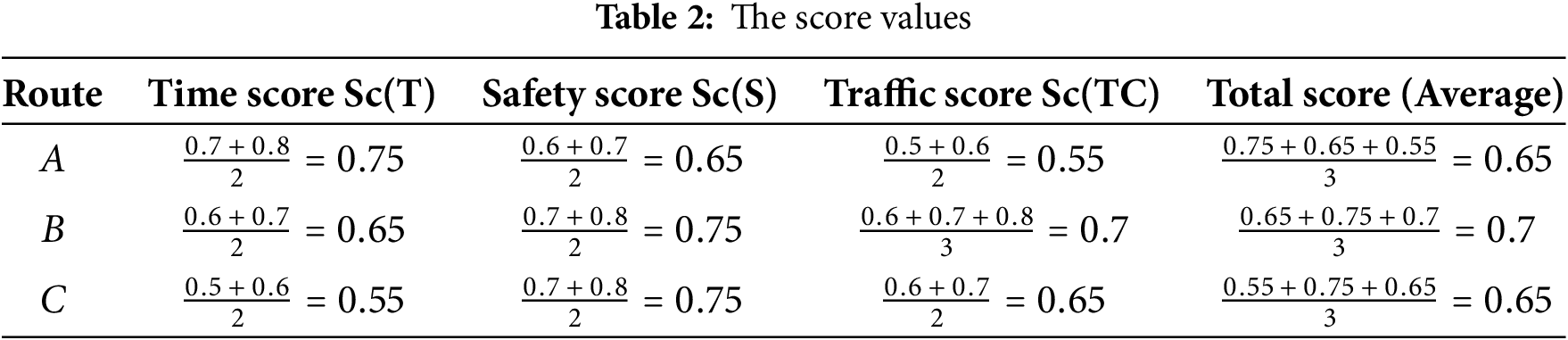
For each hesitant fuzzy set h={v1,v2,...,vn}, we calculate the score function in the following Table 2:
Sc(h)=(1N(h))∑vi∈hvi(14)

Thus the Route B has the highest total score “0.7”.
Step 3: Define the (μ,ν)-Level Set
Choosing (μ,ν) Parameters
let us suppose μ = 0.6 and ν = 0.3.
Definition 12 states that the (μ,ν)-level set of Lˇ is
(Lˇw;e)(μ,ν)={t∈W:Sc((Lˇw;e)(t))≥μ}∪{t∈W:Sc((Lˇw;e)(t))≤ν}
It means that the route satisfying either Sc((Lˇw;e)(t))≥μ or Sc((Lˇw;e)(t))≤ν belongs to the (μ,ν) level set.
Step 4: Identify Routes in the (μ,ν)-Level Set
Routes with Sc((Lˇw;e)(t))≥μ=0.6 are
{A, B, C} and routes with Sc((Lˇw;e)(t))≤ν=0.3 are {}
Thus, the (μ,ν)-level set contains:
(Lˇw;e)(μ,ν)={A,B,C}
Step 5: Identify Hesitant Fuzzy Soft Fixed Points
A hesitant fuzzy soft fixed point u^ is a route such that:
u^∈(Lˇw;e)(μ,ν)
From the (μ,ν)-level set, we see that all routes satisfy the fixed-point condition, meaning: A, B, C are hesitant fuzzy soft fixed points. However, since B has the highest score (0.7), it is the most optimal choice.
Step 6: Decision Making
i) The (μ,ν)-level set contains all three routes.
ii) Since route B has the highest hesitant fuzzy score (0.7), it is the best choice for the selection.
iii) Thus, B is selected as the final route.
Final Conclusion
i) Definition 12 ensures that the best route is within the (μ,ν)-level set.
ii) Hesitant fuzzy soft fixed points guarantee decision stability.
iii) B is the best route, as it has the highest hesitant fuzzy score and belongs to the level set.
The following example shows real world problem solved by Definitions 10 and 11.
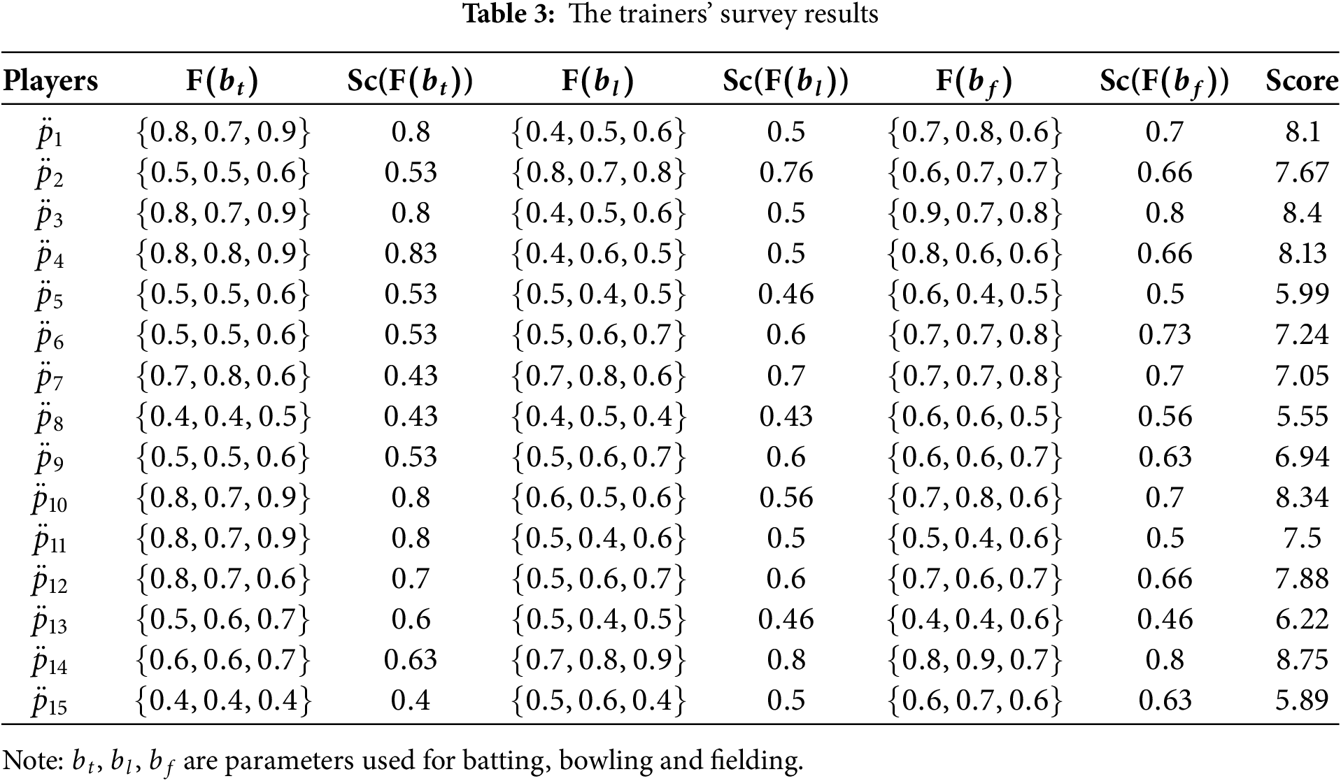
Example 4. Let’s say that a cricket organisation t ravels the nation doing trials to find local talent. Three well-known Test and first-class cricket players, who are also among the top instructors in the sport, have led the tryouts. After 15 players have been chosen, it is agreed to hold a camp for training to choose the top 11 players before the cricket team is finalised. First of all, these three trainers have scheduled a coaching event. After the final trials, these trainers and instructors are asked to serve as assessors by offering their unbiased thoughts. With the use of the hesitant fuzzy soft set theory, let’s examine this event mathematically as follows: W={p¨1,p¨2,p¨3,p¨4,p¨5,p¨6,p¨7,p¨8,p¨9,p¨10,p¨11,p¨12,p¨13,p¨14,p¨15} (set of players) and M⊂E be given by M={bt,bl,bf}, where bt,bl, and bf represents batting, bowling, and fielding, respectively. The three trainers’ opinions, F1,F2, and F3, are represented by the following hesitant fuzzy soft set F:
F(bt)={p¨1/{0.8,0.7,0.9},p¨2/{0.5,0.5,0.6},p¨3/{0.8,0.7,0.9},p¨4/{0.8,0.8,0.9},p¨5/{0.5,0.5,0.6},p¨6/{0.5,0.5,0.6},p¨7/{0.4,0.4,0.5},p¨8/{0.4,0.4,0.5},p¨9/{0.5,0.5,0.6},p¨10/{0.8,0.7,0.9},p¨11/{0.8,0.7,0.9},p¨12/{0.8,0.7,0.6},p¨13/{0.5,0.6,0.7},p¨14/{0.6,0.6,0.7},p¨15/{0.4,0.4,0.4}}.F(bl)={p¨1/{0.4,0.5,0.6},p¨2/{0.8,0.7,0.8},p¨3/{0.4,0.5,0.6},p¨4/{0.4,0.6,0.5},p¨5/{0.5,0.4,0.5},p¨6/{0.5,0.6,0.7},p¨7/{0.7,0.8,0.6},p¨8/{0.4,0.5,0.4},p¨9/{0.5,0.6,0.7},p¨10/{0.6,0.5,0.6},p¨11/{0.5,0.4,0.6},p¨12/{0.5,0.6,0.7},p¨13/{0.5,0.4,0.5},p¨14/{0.7,0.8,0.9},p¨15/{0.5,0.6,0.4}}.F(bf)={p¨1/{0.7,0.8,0.6},p¨2/{0.6,0.7,0.7},p¨3/{0.9,0.7,0.8},p¨4/{0.8,0.6,0.6},p¨5/{0.6,0.4,0.5},p¨6/{0.7,0.7,0.8},p¨7/{0.6,0.7,0.8},p¨8/{0.6,0.6,0.5},p¨9/{0.6,0.6,0.7},p¨10/{0.7,0.8,0.6},p¨11/{0.5,0.4,0.6},p¨12/{0.7,0.6,0.7},p¨13/{0.4,0.4,0.6},p¨14/{0.8,0.9,0.7},p¨15/{0.6,0.7,0.6}}.
Presume that the weights assigned to batting, bowling, and fielding are 5:4:3. In this manner, a player’s ultimate score is determined using the following formula. Score=5Sc(F(bt))+4Sc(F(bl))+3Sc(F(bf)).
This data is presented in Table 3.

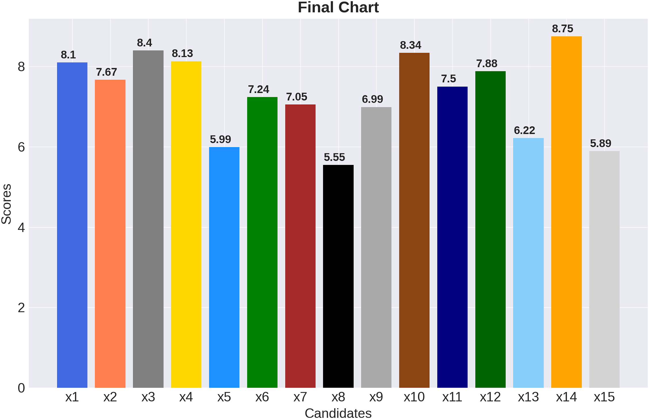
A selection of this data is displayed in the following charts. Each player individual score is represented by Fig. 1. A cursory examination of these charts reveals that p¨1,p¨3,p¨4,p¨10,p¨11 are the best five batsman; p¨2,p¨7,p¨9,p¨12,p¨14 are the best five bowlers; and p¨3,p¨6,p¨14 are the best fielders.

Figure 1: Score for each individual
The following Fig. 2 represents the final score of each player.

Figure 2: Last tally
Here the mid-level decision rule and the mid-level threshold fuzzy set of ΔF is as mid
ΔF={(bt,0.62),(bl,0.5),(bf,0.65)}.
Furthering, we can get the mid-level soft set ΔF={(bt,{p1,p3,p4,p10,p11,p12,p14}),(bl,{p2,p6,p7,p9,p10,p12,p14}) (bf,{p1,p2,p3,p4,p6,p7,p10,p12,p14})}.
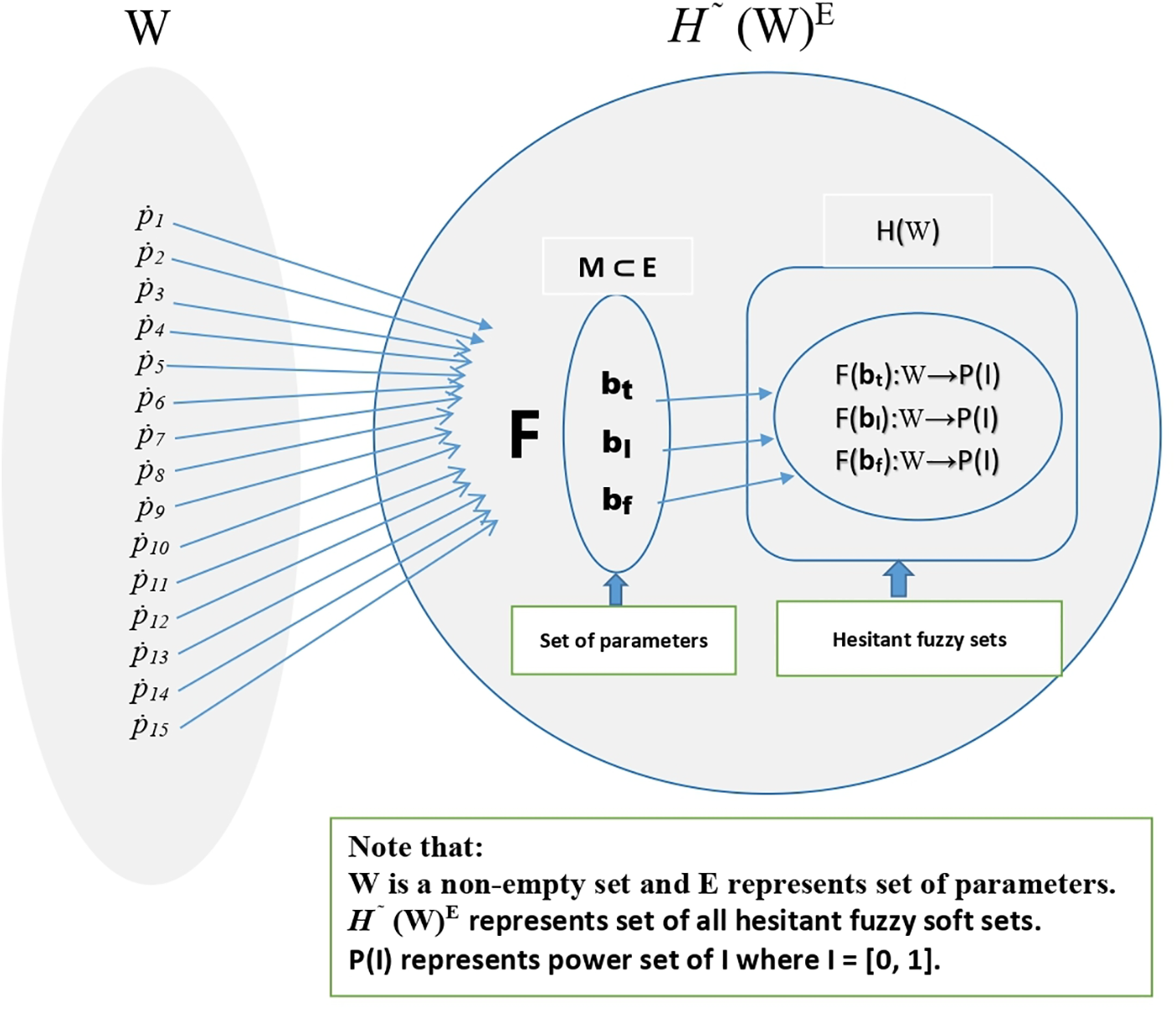
Now let us define hesitant fuzzy soft set valued mapping Lˇ:W→H~(W)E by Lˇ(p)=F;∀,p∈W. For μ=0.62∈(0,1] we note that p14∈Lˇ[p14]0.62 be E-hesitant fuzzy soft fixed point of Lˇ, which is the best player of the team. The above mechanism of the problem is represented by the Fig. 3.
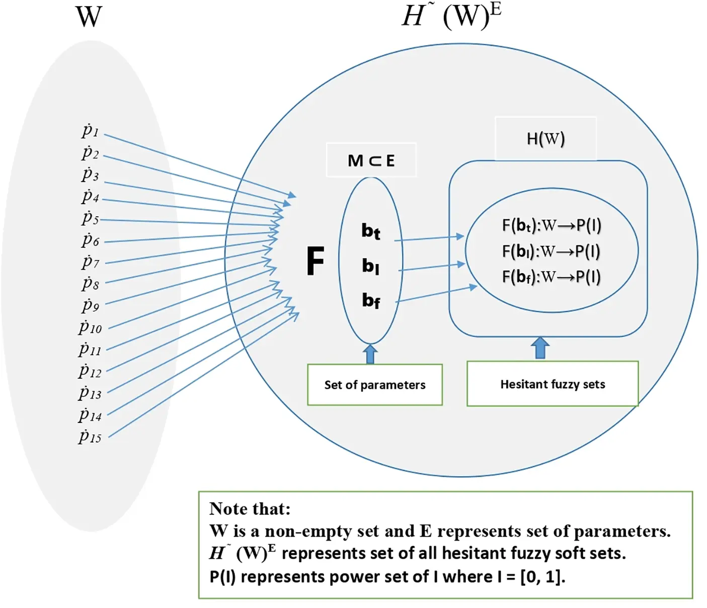
Figure 3: An illustrative representation of a hesitant fuzzy soft set-valued mapping F, where a universal set W is mapped into hesitant fuzzy soft set within H~(W)E. The parameters M⊆E influence the mapping, defining hesitant fuzzy decision components bt, bl, bf, each associated with a power set transformation into P(I)
The above methodology can be summarised in the following Fig. 4. It is clearly shown from the results that hesitant fuzzy soft set mechanism gives us more prominent results as compared to the other mechanisms.
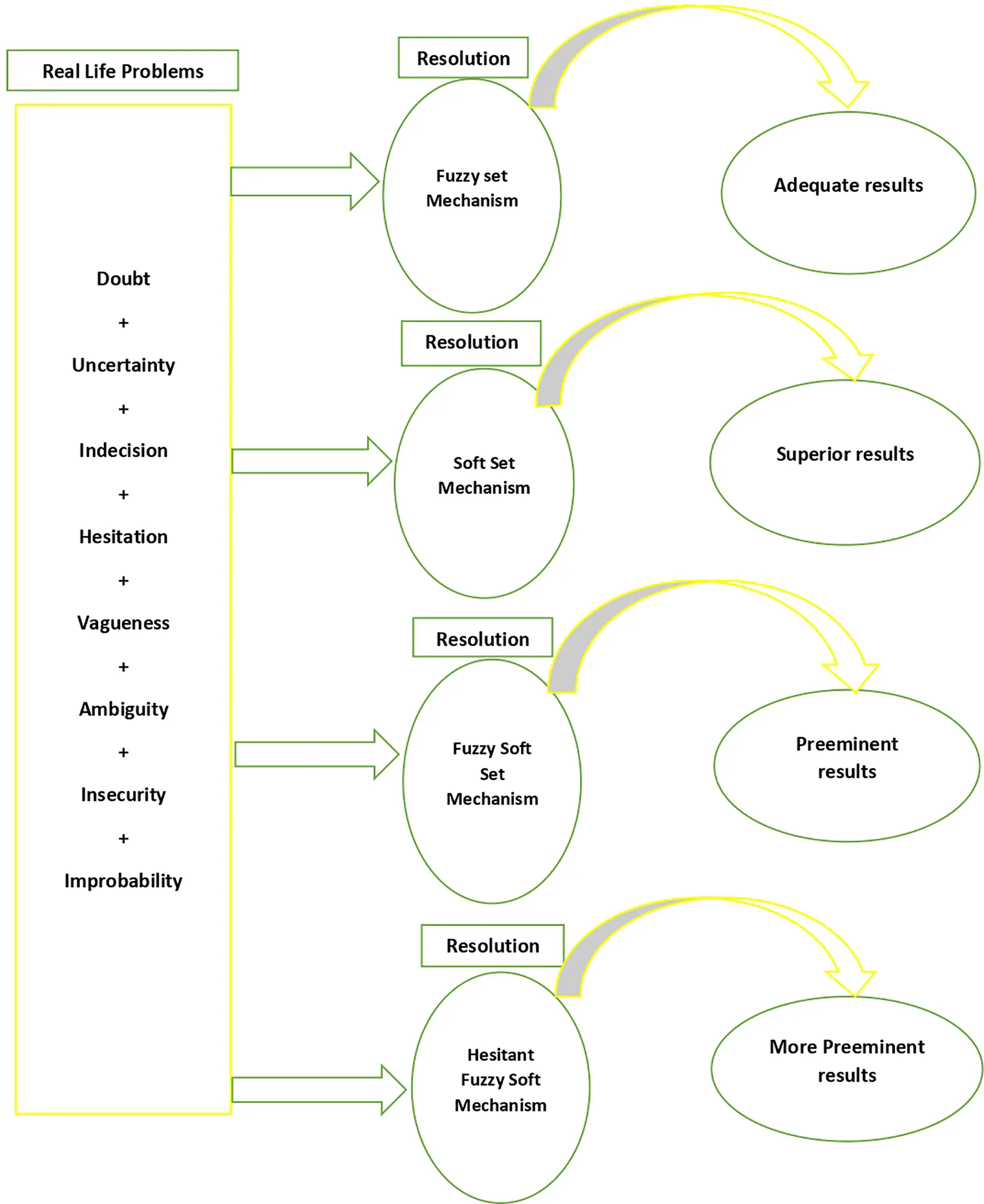
Figure 4: Decision-making methodology
5 Conclusion
Fixed points theory plays a significant role in decision-making problems, particularly in economics, game theory, and optimization. In the context of decision-making problems, fixed points are often used to identify stable solutions. Applications in decision-making issues like risk management and resource allocation show how helpful and reliable the suggested method is. We introduced the Suzuki-type (μ,ν)-weak contraction and hesitant fuzzy soft set valued-mapping. Further, using these concepts, we established some fixed point theorems in the framework of metric spaces. We also solved some decision-making problems based on the presented work. Moreover, these theorems only show the existence of the “hesitant fuzzy soft fixed point.”
The suggested approach assumes the completeness of the metric space and uses Suzuki-Type (μ,ν)-Weak Contraction for hesitant fuzzy soft set-valued mappings. In some real-world applications, especially those involving substantially non-convex or fragmented datasets, this assumption might not hold. To increase the method’s usefulness, future research could examine expansions to quasi-metric spaces or loosen the completeness assumption.
Acknowledgement: The authors Muhammad Sarwar and Kamaleldin Abodayeh are thankful to Prince Sultan University for the support of this manuscript through TAS research lab.
Funding Statement: This research was funded by National Science, Research and Innovation Fund (NSRF), and King Mongkut’s University of Technology North Bangkok with Contract No. KMUTNB-FF-68-B-46.
Author Contributions: Conceptualization, writing—review and editing, Muhammad Sarwar and Rafiq Alam; Supervision, project administration, formal analysis, Muhammad Sarwar and Kamaleldin Abodayeh; Visualization, investigation, funding acquisition, Saowaluck Chasreechai and Thanin Sitthiwirattham; Writing—original draft preparation, data curation, Rafiq Alam. All authors reviewed the results and approved the final version of the manuscript.
Availability of Data and Materials: Not applicable.
Ethics Approval: Not applicable.
Conflicts of Interest: The authors declare no conflicts of interest to report regarding the present study.
References
1. Saeed M, Saif Ud Din I, Tariq I, Garg H. Refined fuzzy soft sets: properties, set-theoretic operations and axiomatic results. J Comput Cogn Eng. 2023;3(1):24–33. doi:10.47852/bonviewJCCE3202847. [Google Scholar] [CrossRef]
2. Liu X. Fuzzy soft expert matrix theory and its application in decision-making. Open J Appl Sci. 2023;13:1403–17. doi:10.4236/ojapps.2023.138111. [Google Scholar] [CrossRef]
3. Bhardwaj N, Sharma P. An advanced uncertainty measure using fuzzy soft sets: application to decision-making problems. Big Data Min Anal. 2021;4(2):94–103. doi:10.26599/BDMA.2020.9020020. [Google Scholar] [CrossRef]
4. Kirisci M. New type pythagorean fuzzy soft set and decision-making application. arXiv:1904.04064. 2019. [Google Scholar]
5. Ali MS, Ghorbani A, Ozyer T. A series of information measures of hesitant fuzzy soft sets and their application in decision making. Soft Comput. 2020;24(10):7107–20. doi:10.1007/s00500-020-05485-4. [Google Scholar] [CrossRef]
6. Xu Z, Cai X. Hesitant fuzzy set: theory and extension. Springer; 2021. doi:10.1007/978-981-16-7301-6. [Google Scholar] [CrossRef]
7. Eftekhari M, Mehrpooya A, Saberi-Movahed F, Torra V. How fuzzy concepts contribute to machine learning. Cham, Switzerland: Springer; 2022. [Google Scholar]
8. Shen Q, Lou J, Liu Y, Jian Y. Hesitant fuzzy multi-attribute decision making based on binary connection number of set pair analysis. Soft Comput. 2021;25(23):14797–807. doi:10.1007/s00500-021-06215-0. [Google Scholar] [PubMed] [CrossRef]
9. Ali G, Afzal A, Sheikh U, Nabeel M. Multi-criteria group decision-making based on the combination of dual hesitant fuzzy sets with soft expert sets for the prediction of a local election scenario. Granul Comput. 2023;8(6):2039–66. doi:10.1007/s41066-023-00414-w. [Google Scholar] [CrossRef]
10. Heilpern S. Fuzzy mappings and fixed point theorem. J Math Anal Appl. 1981;83(2):566–9. doi:10.1016/0022-247X(81)90141-4. [Google Scholar] [CrossRef]
11. Nadler SB. Multi-valued contraction mappings. Pac J Math. 1969;30(2):475–88. doi:10.2140/pjm.1969.30.475. [Google Scholar] [CrossRef]
12. Banach S. Sur les operations dans les ensembles abstraits et leur application aux equations intexgrales. Fund Math. 1922;3(1):133–81. doi:10.4064/fm-3-1-133-181. [Google Scholar] [CrossRef]
13. Frigon M, O’Regan D. Fuzzy contractive maps and fuzzy fixed points. Fuzzy Sets Syst. 2002;129(1):39–45. doi:10.1016/S0165-0114(01)00171-3. [Google Scholar] [CrossRef]
14. Adhya S, Deb Ray A. Common fixed point theorems on complete and weak G-Complete fuzzy metric spaces. arXiv:2111.08938. 2021. [Google Scholar]
15. Mohammed SS. On Bilateral fuzzy contractions. Funct Anal Approx Comput. 2020;12(1):1–13. [Google Scholar]
16. Mohammed SS, Awam A. Fixed points of soft-set valued and fuzzy set-valued maps with applications. J Intell Fuzzy Syst. 2019;37(3):3865–77. doi:10.3233/JIFS-190126. [Google Scholar] [CrossRef]
17. Ahmad J, Aydi H, Mlaiki N. Fuzzy fixed points of fuzzy mappings via F-contractions and an application. J Intell Fuzzy Syst. 2019;37(4):5487–93. doi:10.3233/JIFS-190580. [Google Scholar] [CrossRef]
18. Ali B, Ali H, Nazir T, Ali Z. Existence of fixed points of suzuki-type contractions of quasi-metric spaces. Mathematics. 2023;11(21):4445. doi:10.3390/math11214445. [Google Scholar] [CrossRef]
19. Doric D, Lawovic R. Some Suzuki-type fixed point theorems for generalized multivalued mappings and applications. Fixed Point Theory Appl. 2011;40(1):1861. doi:10.1186/1687-1812-2011-40. [Google Scholar] [CrossRef]
20. Qawaqneh HA, Noorani MS, Shatanawi W. Fixed point results for geraghty type generalized F-contraction for weak alpha-admissible mapping in metric-like spaces. Eur J Pure Appl Math. 2018;11(3):702–16. doi:10.29020/nybg.ejpam.v11i3.3294. [Google Scholar] [CrossRef]
21. Qawaqneh HA, Noorani MS, Shatanawi W. Fixed point theorem for (α, k, υ)-contractive multi-valued mapping in b-metric space and applications. Int J Math Comput Sci. 2019;14(1):263–83. [Google Scholar]
22. Shagari MS, Noorwali M, Awam A. Hybrid fixed point theorems of fuzzy soft set-valued maps with applications in integral inclusions and decision making. Mathematics. 2023;11(6):1393. doi:10.3390/math11061393. [Google Scholar] [CrossRef]
23. Shagari MS, Awam A. Fixed points of hesitant fuzzy set-valued maps with applications. Carpathian Math Publ. 2021;13(3):711–26. doi:10.15330/cmp.13.3.711-726. [Google Scholar] [CrossRef]
24. Driguew RM, Martinew L, Torra V, Xu ZS, Herrera F. Hesitant fuzzy sets: state of the art and future directions. Int J Intell Syst. 2014;29(6):495–524. doi:10.1002/int.21654. [Google Scholar] [CrossRef]
25. Ciric LB. Fixed points for generalized multi-valued contractions. Mat Vesnik. 1972;9(24):265–72. [Google Scholar]

 Submit a Paper
 Propose a Special lssue
 Open Access
 View Full Text
 Download PDF
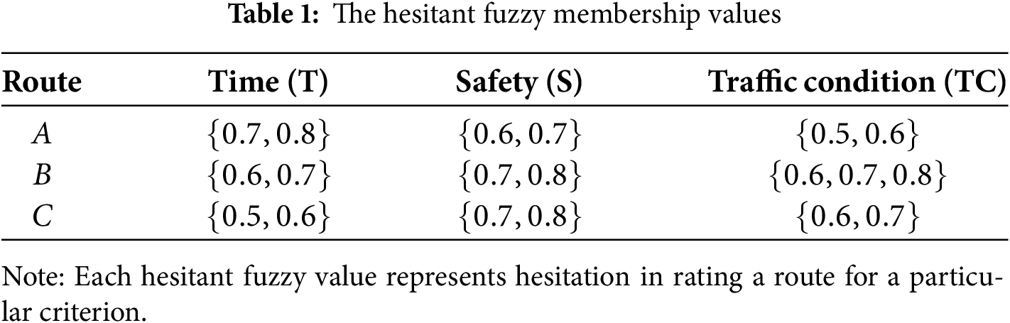


 Copyright © 2025 The Author(s). Published by Tech Science Press.
 Downloads
 Citation Tools