Analytical Solutions for 1-Dimensional Peridynamic Systems by Considering the Effect of Damping

1  Introduction

As a new continuum mechanics formulation, peridynamics [1–4] has been developed by considering the limitations of classical continuum mechanics, which is formulated in the form of partial differential equations. Along the discontinuities, such as cracks, spatial derivatives are not defined as part of the partial differential equations. The peridynamics equation of motion is given in integro-differential equation form, which does not contain any spatial derivatives and is valid with or without discontinuities. In addition, classical continuum mechanics does not have a length scale parameter, which can be necessary when analyzing advanced material systems with microstructural details. On the other hand, peridynamics has an important parameter named the horizon, which is the length scale parameter. With the horizon approaching zero, peridynamics equations can converge to classical continuum mechanics equations.

During the last ten years, there has been rapid progress in peridynamics research. For instance, peridynamics has been successfully utilized for the analysis of many different material systems. Liu et al. [5] introduced a modified rate-dependent peridynamic model to investigate the dynamic mechanical behavior of ceramic materials. Chen et al. [6] introduced a refined thermo-mechanical fully coupled peridynamic model and investigated fracture in concrete. By performing peridynamic simulations, Shi et al. [7] examined damage evolution in reinforced concrete subjected to radial blasting. Ma et al. [8] proposed an improved peridynamic model for the quasi-static and dynamic fracture of reinforced concrete. Wang and Wu [9] presented a bond-level energy-based peridynamic model for mixed-mode fracture in rocks. Wu et al. [10] performed peridynamic failure analysis in a Ni/Ni3Al bi-material structure. Chunyu et al. [11] developed a numerical model to simulate a dynamic ice-milling process by using state-based peridynamics. Yang et al. [12] presented a peridynamic formulation suitable for out-of-plane damage analysis of composite laminates. Oterkus and Madenci [13] showed the application of peridynamics for failure prediction in composites. In another study, Oterkus et al. [14] predicted damage growth from loaded composite fastener holes by using peridynamics. To investigate fracture behavior in nuclear fuel pellets, Liu et al. [15] developed a thermomechanical peridynamic model. By using element-based peridynamics, Jiang et al. [16] analyzed functionally graded materials. Diana et al. [17] used peridynamics to determine homogenized properties for microstructured materials. Yin et al. [18] developed a peridynamic model for large deformation and fracture analysis of hyperelastic materials.

Peridynamic formulations for simplified structures are also available in the literature. O’Grady and Foster [19] developed a peridynamic beam formulation within a non-ordinary state-based peridynamic framework. Three-dimensional Euler-Bernoulli beam structures were studied by Liu et al. [20] using an element-based peridynamic model. Chen et al. [21] performed a peridynamic fatigue crack growth analysis of hydrogels. To predict the initiation and propagation of cracks in brittle solids Wang et al. [22] presented a 3-D conjugated bond-pair-based peridynamic formulation.

Peridynamics can also be utilized to analyze different types of material responses, including elastic, plastic, viscoelastic, and viscoplastic material behavior. Zu et al. [23] presented an elastoplastic fracture model in a bond-based peridynamic framework. Liu et al. [24] proposed a time-discontinuous state-based peridynamic formulation for elastoplastic dynamic fracture problems. A viscoelastic model of non-ordinary state-based peridynamics was developed by Tian and Zhou [25]. Zhang et al. [26] introduced a peridynamic approach to model elasto-viscoplastic ductile fracture. A new ordinary state-based peridynamic framework was proposed by Zhang et al. [27], including the Drucker-Prager plasticity model and shear deformation.

The meshless approach is usually used for the solution of peridynamic equations of motion instead of utilizing semi-analytical [28] or mesh-based approaches. There are also some analytical solutions available in the literature. Amongst these, Mikata presented analytical solutions for peristatic and peridynamic problems for a 1-dimensional infinite rod [29] and 3-dimensional isotropic materials [30]. Yang et al. demonstrated an analytical solution of 1-dimensional [31] and 2-dimensional [32] peridynamic equations of motion.

This study introduces a novel analytical solution for 1-dimensional peridynamic systems by considering the effect of damping, which can occur due to internal losses in the material, friction in joints, and others. After demonstrating the details of the analytical solution, various demonstration problems are considered. Peridynamic analytical results and results obtained from the classical theory are compared against each other. In addition, the effect of the horizon as the length scale parameter is demonstrated.

2  Analytical Solution of 1-Dimensional Peristaltic Governing Equation

For a 1-dimensional bar, the peristatic governing equation is described as follows:

c∫−δδu(x+ξ)−u(x)|ξ|dξ=−b(x)c=2EAδ2(1)

where c is the bond constant, u(x) is the displacement of the material point located at x, b(x) is the body load, ξ is the bond length, E is the Elastic Modulus, and A is the cross-sectional area, and δ is the size of the horizon.

With the introduction of fictitious regions outside the boundary, clamped and free boundary conditions can be written as follows (Appendix A):

clamped:u(x∗−ξ)=−u(x∗+ξ)free:u(x∗−ξ)=u(x∗+ξ)∀ξ∈[0,δ](2)

where x* is the location of the boundary condition.

2.1 Clamped-Clamped Condition

For a clamped-clamped bar subjected to some arbitrary loading, the boundary conditions are given as

u(−ξ)=−u(ξ)  and  u(L+ξ)=−u(L−ξ)∀ξ∈[0,δ](3)

where L is the length of the bar.

Selecting the trial function as follows:

u(x)=∑n=1∞ansin⁡nπxL(4)

where an is an unknown coefficient and substituting Eq. (4) into Eq. (1) gives

c∑n=1∞an∫−δδ1|ξ|(1−cos⁡nπξL)dξsin⁡nπxL=b(x)(5)

Unknown coefficients in Eq. (5) can be determined using the orthogonality condition as follows:

an=2cL∫0Lb(x)sin⁡nπxLdx∫−δδ1|ξ|(1−cos⁡nπξL)dξ(6)

Substituting Eq. (6) back into Eq. (4) results in the peristatic analytical solution for a clamped-clamped bar as follows:

u(x)=2cL∑n=1∞∫0Lb(x)sin⁡nπxLdx∫−δδ1|ξ|(1−cos⁡nπξL)dξsin⁡nπxL(7)

2.2 Clamped-Free Condition

For a bar that is only clamped at the left end, the boundary conditions can be described as follows:

u(−ξ)=−u(ξ)and u(L+ξ)=u(L−ξ)∀ξ∈[0,δ](8)

In this case, the trial function can be chosen as follows:

u(x)=∑n=1∞bnsin⁡(2n−1)πx2L(9)

where bn is an unknown coefficient. Substituting Eq. (9) into Eq. (1) and after simplification yields

c∑n=1∞bn∫−δδ1|ξ|[1−cos⁡(2n−1)πξ2L]dξsin⁡(2n−1)πx2L=b(x)(10)

Coefficients in Eq. (10) can be obtained using the orthogonality condition as follows:

bn=2cL∫0Lb(x)sin⁡(2n−1)πx2Ldx∫−δδ1|ξ|[1−cos⁡(2n−1)πξ2L]dξ(11)

Therefore, the peristatic analytical solution for this case can be written as:

u(x)=2cL∑n=1∞∫0Lb(x)sin⁡(2n−1)πx2Ldx∫−δδ1|ξ|[1−cos⁡(2n−1)πξ2L]dξsin⁡(2n−1)πx2L(12)

3  Analytical Solution of 1-Dimensional Peridynamic Equation of Motion by Considering the Effect of Damping

In general, the peridynamic (PD) equation of motion for a 1-dimensional bar can be written as follows:

ρu¨(x,t)+du˙(x,t)=c∫−δδu(x+ξ,t)−u(x,t)|ξ|dξ+b(x,t)(13)

where ρ is density, d is the damping factor, t represents time, “.” is the derivative of a function for time, and “..” is the second derivative of a function with respect to time.

Suppose the initial conditions are known as follows:

u(x,0)=u0(x)and u˙(x,0)=v0(x)(14)

And if the Laplace transform for the time variable t:

L[u(x,t)]=U(x,s)  and  L[b(x,t)]=B(x,s)(15)

Thus, applying the Laplace transform to both sides of Eq. (13) in t results in

ρ[s2U(x,s)−su0(x)−v0(x)]+d[sU(x,s)−u0(x)]=c∫−δδU(x+ξ,s)−U(x,s)|ξ|dξ+B(x,s)(16)

Rearranging Eq. (16) gives

c∫−δδU(x+ξ,s)−U(x,s)|ξ|dξ=s2ρU(x,s)+s[dU(x,s)−ρu0(x)]−ρv0(x)−du0(x)−B(x,s)(17)

3.1 Clamped-Free Condition

For the clamped-free case, comparing Eq. (17) with Eq. (1) yields:

c∫−δδU(x+ξ,s)−U(x,s)|ξ|dξ=−{ρv0(x)+du0(x)+B(x,s)−s2ρU(x,s)−s[dU(x,s)−ρu0(x)]}c∫−δδu(x+ξ)−u(x)|ξ|dξ=−b(x)(18)

Considering U(x,s) as an analogue to u(x) leads to:

U(x,s)=∑n=1∞An(s)sin⁡n^x   n^=(2n−1)π2L(19)

Referring to Eq. (10), substituting Eq. (19) into Eq. (18a) yields:

∑n=1∞An(s)[c∫−δδ1|ξ|(1−cos⁡n^ξ)dξ+s2ρ+sd]sin⁡n^x=ρv0(x)+du0(x)+B(x,s)+sρu0(x)(20)

Coefficients in Eq. (20) can be determined using the orthogonality condition as follows:

An(s)=2L1ρρv^0(n)+du^0(n)+∫0LB(x,s)sin⁡n^xdx+sρu^0(n)(s−α1(n))(s−α2(n))(21)

where

u^0(n)=∫0Lu0(x)sin⁡n^xdx  and  v^0(n)(x)=∫0Lv0sin⁡n^xdx

with

α1(n)=−d+d2−4ρc∫−δδ1|ξ|(1−cos⁡n^ξ)dξ2ρ=−ηnωn+ωn(ηn)2−1α2(n)=−d−d2−4ρc∫−δδ1|ξ|(1−cos⁡n^ξ)dξ2ρ=−ηnωn−ωn(ηn)2−1(22)

ωn=cρ∫−δδ1|ξ|(1−cos⁡n^ξ)dξ  and  ηn=d2ρωn

It can be rewritten using partial fractions in Eq. (21) as

An(s)=2L1ρ{ρv^0(n)+du^0(n)α1(n)−α2(n)(1s−α1(n)−1s−α2(n))+ρu^0(n)α1−α2(α1(n)s−α1(n)−α2(n)s−α2(n))+∫0LB(x,s)sin⁡n^xdx(s−α1(n))(s−α2(n))}(23)

Recalling the following and applying the inverse Laplace transform to Eq. (23) yields Eq. (25).

L−1(1s−α)=eαt  and  L−1[F(s)G(s)]=(f∗g)(t)=∫0tf(u)g(t−u)du(24)

an(t)=2L1ρ1α1(n)−α2(n){(ρv^0(n)+du^0(n))(eα1(n)t−eα2(n)t)+ρu^0(n)(α1eα1(n)t−α2eα2(n)t)+∫0t(eα1(n)u−eα2(n)u)[∫0Lb(x,t−u)sin⁡n^xdx]du}(25)

where the following is the solution to this case:

u(x,t)=L−1[U(x,s)]=∑n=1∞an(t)sin⁡n^x(26)

Substituting Eq. (25) into Eq. (26) yields:

u(x,t)=2L∑n=1∞1α1(n)−α2(n){[(v^0(n)+dρu^0(n))+u^0α1]eα1(n)t−[(v^0(n)+dρu^0(n))+u^0α2]eα2(n)t+1ρ∫0t(eα1(n)u−eα2(n)u)[∫0Lb(x,t−u)sin⁡(n^x)dx]du}sin⁡(n^x)(27)

where

u^0(n)=∫0Lu0(x)sin⁡(n^x)dxv^0(n)(x)=∫0Lv0sin⁡(n^x)dxα1(n)=−ηnωn+ωn(ηn)2−1α2(n)=−ηnωn−ωn(ηn)2−1ωn(δ)=cρ∫−δδ1|ξ|[1−cos⁡(n^ξ)]dξηn=d2ρωnn^=(2n−1)π2Lc=2EAδ2(28)

In particular, for a damped free system, i.e., d=0 and Eqs. (27) and (28) reduce to

u(x,t)=2L∑n=1∞1ωn{v^0(n)sin⁡ωnt+u^0(n)ωncos⁡ωnt+1ρ∫0tsin⁡ωnu[∫0Lb(x,t−u)sin⁡(n^x)dx]du}sin⁡(n^x)(29)

in which

u^0(n)=∫0Lu0(x)sin⁡(n^x)dxv^0(n)(x)=∫0Lv0sin⁡(n^x)dxωn(δ)=cρ∫−δδ1|ξ|[1−cos⁡(n^ξ)]dξn^=(2n−1)π2Lc=2EAδ2(30)

For a bar with clamped-free boundary conditions, the analytical solution has the same form except n^=nπL other than n^=(2n−1)π2L for Eqs. (27) to (29). Particular to the resonance condition, consider a damped-free bar subjected to some harmonic load at an arbitrary point x0, as shown in Fig. 1.

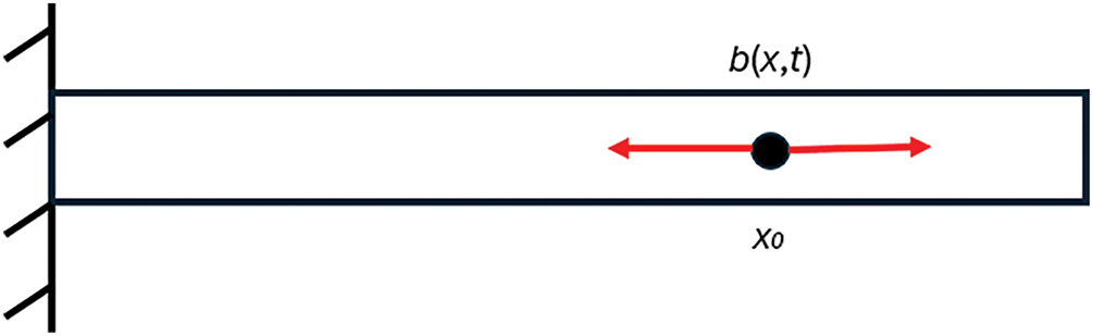
Figure 1: A damped-free bar subjected to some harmonic load at an arbitrary point x0

If the loading frequency coincides with some natural frequencies of the bar, such that

b(x,t)=b0δ(x−xo)sin⁡ωmtm=1,2,3,…(31)

Substituting Eq. (31) into Eq. (27) results in the following:

u(x,t)=2L∑n=1∞1ωn{v^0(n)sin⁡ωnt+u^0(n)ωncos⁡ωnt+1ρ∫0tsin⁡ωnu[∫0Lb0δ(x−xo)sin⁡ωm(t−u)sin⁡(n^x)dx]du}sin⁡(n^x)=2L∑n=1∞1ωn{v^0(n)sin⁡ωnt+u^0(n)ωncos⁡ωnt+1ρb0sin⁡(n^x0)∫0tsin⁡(ωnu)sin⁡[ωm(t−u)]du}sin⁡(n^x)=2L{∑n=1n≠m∞1ωn[v^0(n)sin⁡ωnt+u^0(n)ωncos⁡ωnt+b0ρsin⁡(n^x0)ωmsin⁡ωnt−ωnsin⁡ωmtωm2−ωn2]sin⁡n^x+1ωm[v^0(m)sin⁡ωmt+u^0(m)ωmcos⁡ωmt+b0ρsin⁡(m^x0)sin⁡ωmt−ωmtcos⁡ωmt2ωm]sin⁡m^x}(32)

As t→∞, Eq. (32) diverges.

4  Numerical Cases

To demonstrate the capability of the proposed approach, various scenarios are considered. Peridynamics results and the corresponding classical solutions are compared against each other for validation purposes. A clamped-free bar with Young’s modulus of E=200 GPa, density of ρ=0.785 kg/m, length of L=1m, cross-sectional area of A=0.01×0.01m2, and PD horizon of δ=0.001m are selected for the cases given below.

4.1 Free Vibration of a Damped System

First, the free vibration behavior of a damped system is investigated. Suppose the initial conditions are given as follows:

u0(x)=0.01xv0(x)=10x(x−1)(33)

4.1.1 Case 1: Under Damped

A damping factor of d=1000 Ns/m2 is considered in the first case. Fig. 2 depicts the variation of the displacement at the center of the bar, i.e., x = 0.5 m, with respect to time. It indicates that oscillatory behavior is observed where the amplitude of the displacements decreases due to the effect of damping. Peridynamic results agree very well with the classical solution.

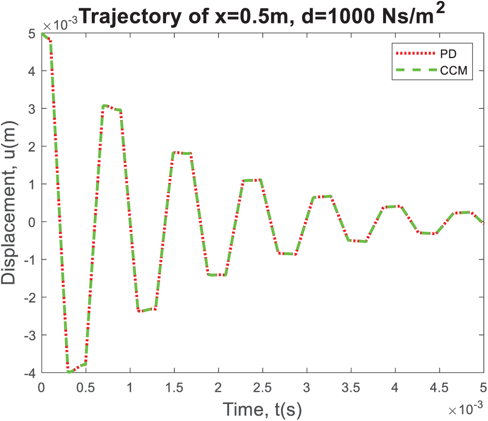
Figure 2: The displacement variation at the center of the bar, i.e., x = 0.5 m, as the time progresses

4.1.2 Case 2: Critically Damped

The damping factor is specified as d=2ρω1=1.2448×104 Ns/m2 in the second case. Concerning the first case, the damping factor is relatively high. Fig. 3 indicates that the system is damped quickly rather than showing an oscillatory behavior, and peridynamic results agree very well with the classical solution.

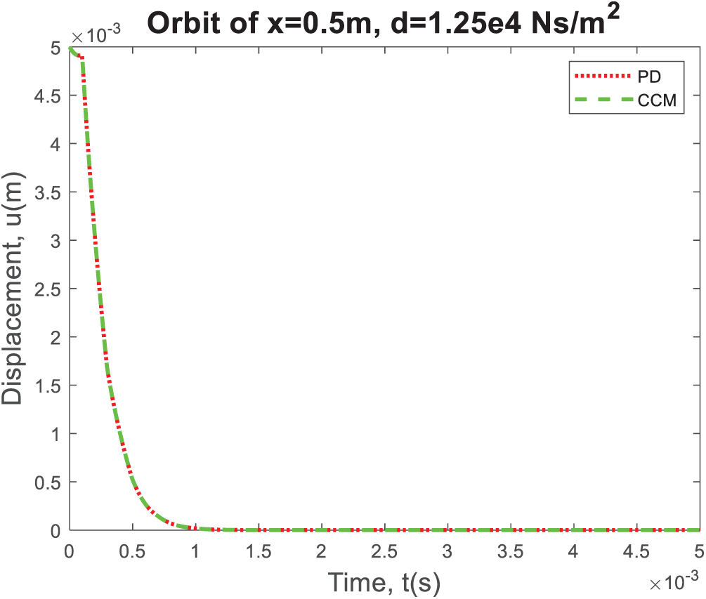
Figure 3: The displacement variation at the center of the bar, i.e., x = 0.5 m, as time progresses

4.2 Forced Oscillation of Undamped System (Non-Resonant)

In this case, a bar that is initially at rest is subjected to a harmonic loading condition exerted at the free end (Fig. 4):

b(x,t)=b0δ(x−L)sin⁡ω¯tω¯=ω12  b0=1000(34)

Figure 4: A bar that is initially at rest is subjected to a harmonic loading condition at the free end

For this particular loading condition, an oscillatory behavior is observed, as shown in Fig. 5, since there is damping in the system, and there is a very good agreement between peridynamic and classical results.

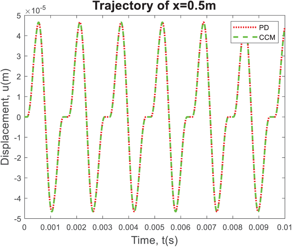
Figure 5: The displacement variation at the center of the bar, i.e., x = 0.5 m, as time progresses

4.3 Forced Vibration of a Damped System

This case is similar to the previous case by including damping in the system, as shown in Fig. 6.

b(x,t)=b0δ(x−L)sin⁡ω¯tω¯=ω12b0=1000  and  d=1000 Ns/m2(35)

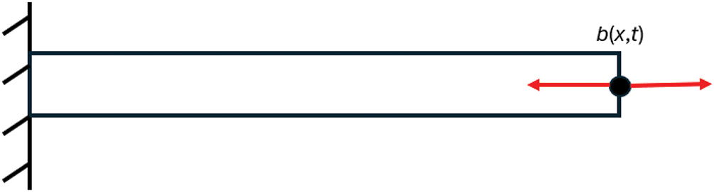
Figure 6: A damped system subjected to forced vibration

Variation of the displacement at the center of the bar, i.e., x = 0.5 m, as time progresses, as shown in Fig. 7. Different from the previous case, the amplitude of oscillations decreases due to damping. There is a very good agreement between peridynamic and classical results.

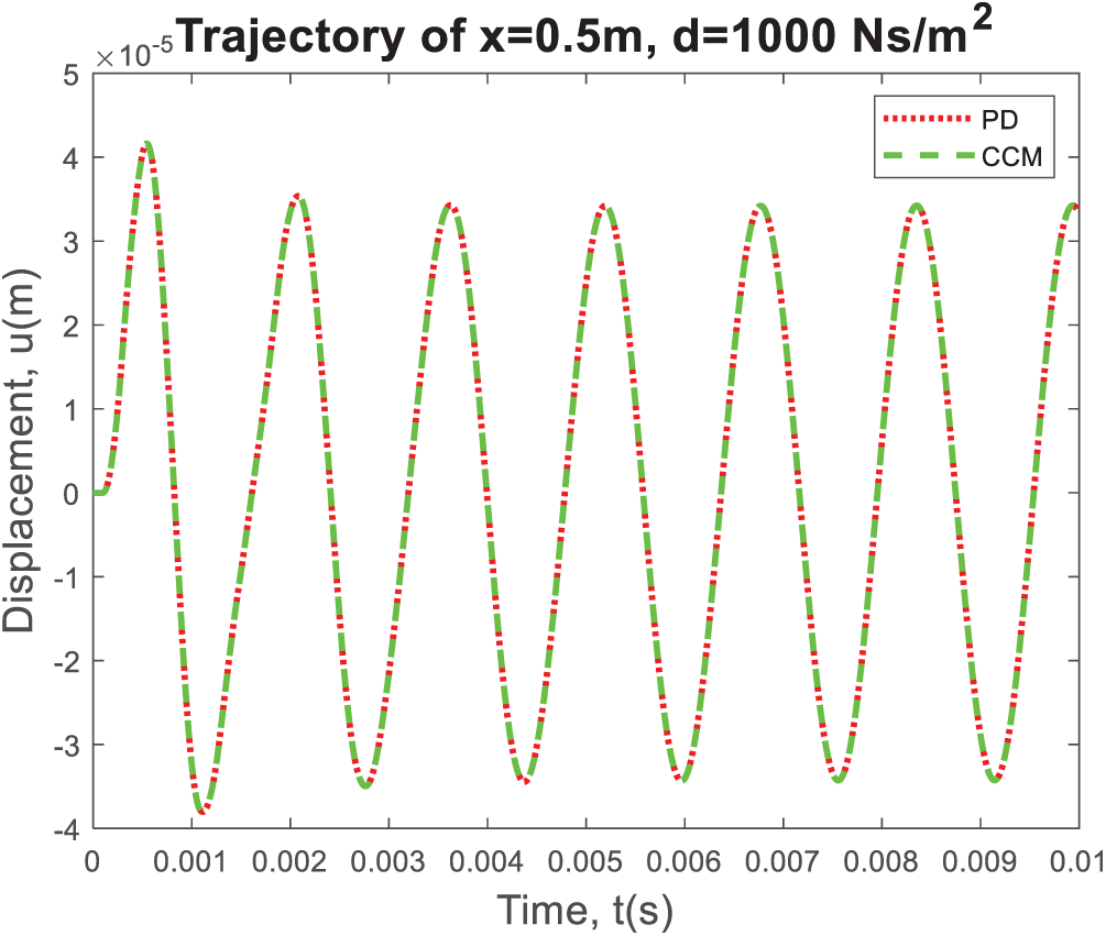
Figure 7: The displacement variation at the center of the bar, i.e., x = 0.5 m, as the time progresses

4.4 Horizon Size Analysis (Natural Frequencies)

The above results indicate that PD agrees with classical theory in oscillation behaviors. However, those solutions are obtained for a small horizon size (δ≪L) so that the nonlocal character does not play a significant role. It can compare the natural frequencies between peridynamics and classical theory by considering different horizon sizes to investigate the subtlety of the nonlocal effect. The natural frequencies from peridynamics are obtained from Eq. (30).

In this case, the horizon size, δ, is varied from 0.0001 to 0.1m. The natural frequencies of the first four modes (n = 1, 2, 3, 4) are shown in Fig. 8. Each mode corresponds to an independent motion of the structure.

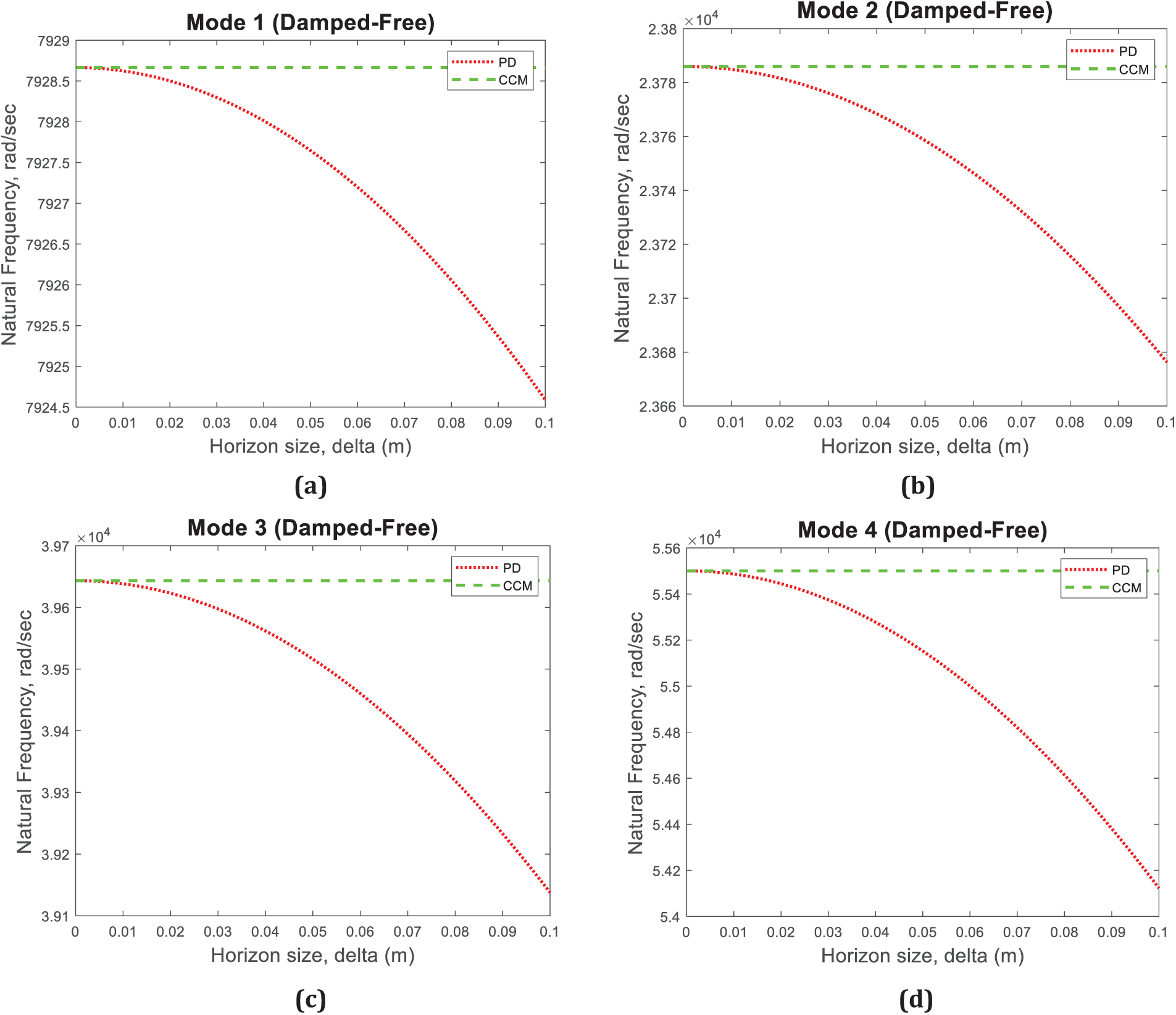
Figure 8: Variation of the natural frequencies as the horizon size changes for (a) Mode 1, (b) Mode 2, (c) Mode 3, and (d) Mode 4

Wang et al. [33] reported that as the horizon size converges to 0 the peridynamic solution should converge to the classical continuum mechanics solution for the condition without the existence of damage in the structure, and nonlocal effects are insignificant. In addition, as indicated in [34], peridynamics can also represent wave dispersion, especially at short wavelengths, which is a phenomenon observed in real materials. For such conditions, the horizon can be determined by comparing the peridynamic wave dispersion curves against those obtained from lattice dynamics. As expected, peridynamic results converge to classical results as the horizon size approaches zero and diverge as the horizon size increases, which can represent non-classical nonlocal behavior that can occur, especially at small scales (see Fig. 8).

4.5 Resonance Analysis

In the last numerical case, a bar subjected to a harmonic load at the free end is considered without the damping effect (Fig. 9). If the loading frequency coincides with the first natural frequency, such as

b(x,t)=b0δ(x−L)sin⁡ω1tb0=100

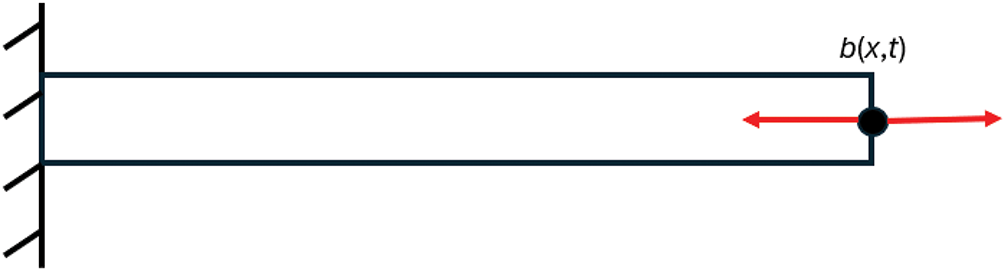
Figure 9: A rod subjected to a harmonic load at the free end without a damping effect

And the bar is initially at rest, i.e.,

u(x,0)=0v˙(x,0)=0

The natural frequencies in PD are functions of the horizon size δ. In this study, two different scenarios for external loading are chosen as follows:

ω1(δ=0.001m)=cρ∫−0.0010.0011|ξ|[1−cos⁡(π2Lξ)]dξω1(δ=0.5m)=cρ∫−0.50.51|ξ|[1−cos⁡(π2Lξ)]dξ

The displacement variation at the right edge of the bar, i.e., x = 1 m, for two different horizon sizes, 0.001 and 0.5 m, as the time progresses obtained by PD and classical theory are shown in Fig. 10. It can observe that both PD and classical theory results show resonant oscillation condition as the amplitude of oscillations increases as the time increases. In particular, for a loading frequency corresponding to a smaller horizon size, the resonance behavior obtained from the PD model and that of Classical Continuum Mechanics (CCM) is similar. In contrast, for a larger horizon size, the resonance of classical theory behaves more weakly than PD. This is expected since natural frequencies of PD converge to classical results for small horizon sizes and deviate from classical results as the horizon size increases, as indicated in Section 4.4.

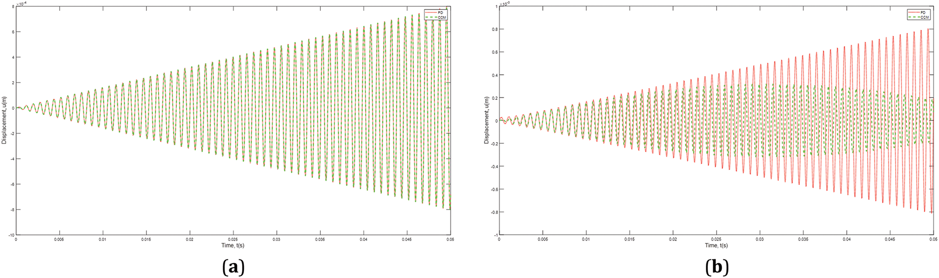
Figure 10: The displacement variation at the right edge of the bar, i.e., x = 1 m, as the progresses for two different horizon sizes (a) 0.001 m, (b) 0.5 m

4.6 Convergence Analysis of the PD Series Solution

This section presents the convergence analysis of the PD series solution for the free vibration of a fixed-free rod by considering the following initial conditions:

u0(x)=0.01xv0(x)=0

The corresponding CCM solution truncated at the first 100 terms is chosen as the base reference:

uCCM(x,t)=∑n=1100[2L∫0L0.01αsin⁡(2n−12Lπα)dα]cos⁡(2n−12LEρπt)sin⁡(2n−12Lπx)

A small horizon of δ=10−4m is selected for the peridynamic solution. The variation of the displacement of the material point at the right edge of the bar with respect to the number of terms in the PD series solution at different times, 0.01, 0.015, 0.02, and 0.025 s, is shown in Fig. 11.

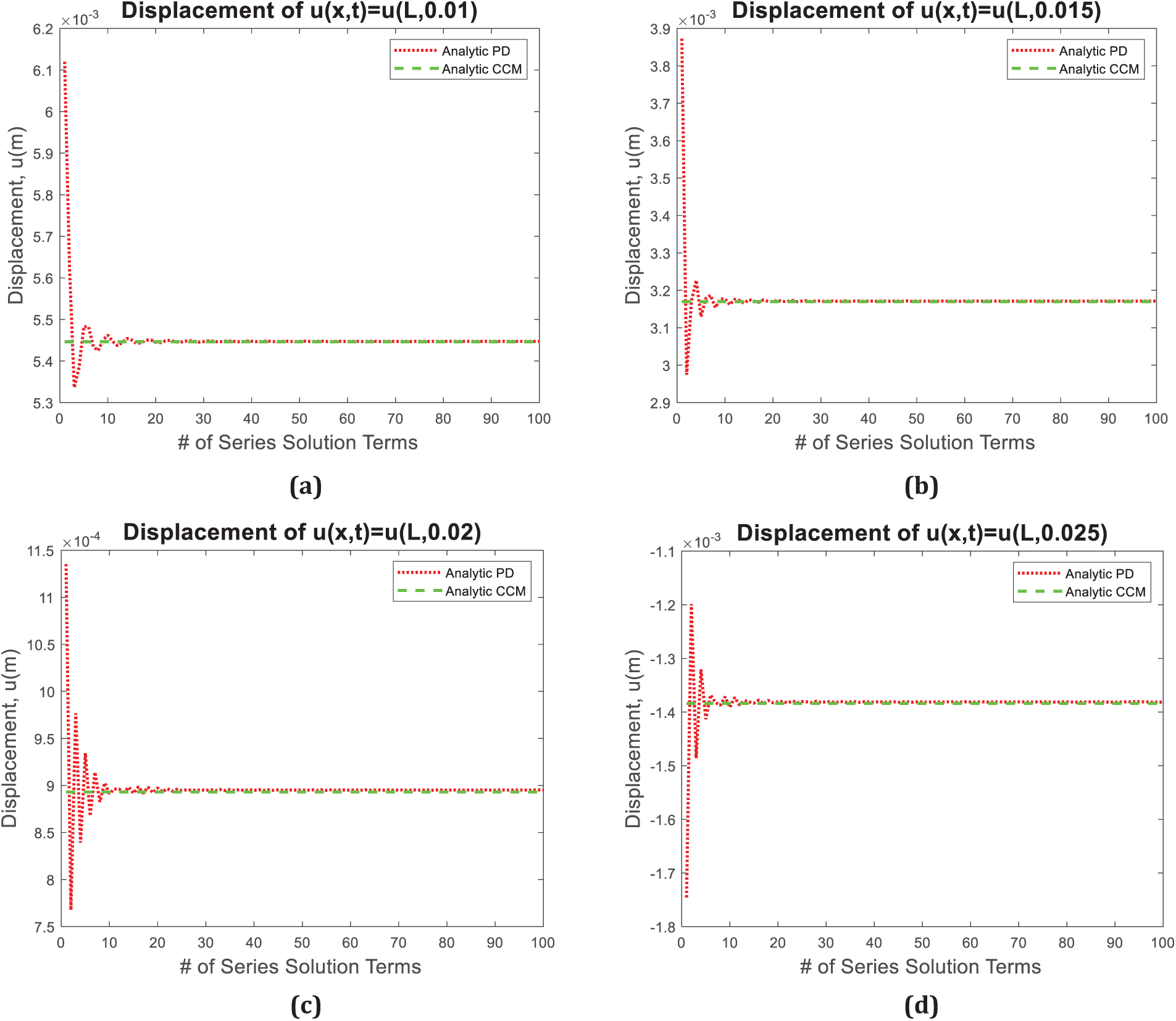
Figure 11: The displacement variation at the right edge of the bar, i.e., x = 1 m, with respect to the number of terms in PD series solution at difference times (a) 0.01 s, (b) 0.015 s, (c), 0.02 s, and (d) 0.025 s

Fig. 11 indicates that the PD solution converges to the CCM solution by using more than 10 terms in the PD series solution.

5  Conclusions

This study presents a novel analytical solution for 1-Dimensional peridynamic systems by considering the effect of damping. After demonstrating the details of the analytical solution, various demonstration problems are given. First, the free vibration of a damped system is considered for under-damped and critically damped conditions. Peridynamic solutions and results from the classical theory are compared against each other, and an excellent agreement is observed between the two approaches. Next, forced vibration analyses of undamped and damped conditions are performed. In addition, the effect of horizon size is investigated. For smaller horizon sizes, peridynamic results agree well with classical results, whereas results from these two approaches deviate from each other as the horizon size increases. In addition, it was presented that using more than 10 terms in the PD series solution, a good convergence is obtained by comparing it against the CCM solution.

Finally, the proposed analytical solution can be utilized for optimization studies as a quick solution without relying on numerical solutions. In addition, the proposed approach can be extended to 2-dimensional and 3-dimensional configurations.

Acknowledgement: None.

Funding Statement: The authors received no specific funding for this study.

Author Contributions: The authors confirm their contribution to the paper as follows: Conceptualization, Zhenghao Yang, Erkan Oterkus, Selda Oterkus, and Konstantin Naumenko; methodology, Zhenghao Yang, Erkan Oterkus, Selda Oterkus, and Konstantin Naumenko; software, Zhenghao Yang; validation, Zhenghao Yang; formal analysis, Zhenghao Yang; investigation, Zhenghao Yang, Erkan Oterkus, Selda Oterkus, and Konstantin Naumenko; data curation, Zhenghao Yang; writing—original draft preparation, Zhenghao Yang; writing—review and editing, Erkan Oterkus, Selda Oterkus, and Konstantin Naumenko; visualization, Zhenghao Yang; supervision, Erkan Oterkus, Selda Oterkus, and Konstantin Naumenko. All authors reviewed the results and approved the final version of the manuscript.

Availability of Data and Materials: The data that support the findings of this study are available from the corresponding author, Erkan Oterkus, upon reasonable request.

Ethics Approval: Not applicable.

Conflicts of Interest: The authors declare no conflicts of interest to report regarding the present study.

Appendix A

Clamped Boundary

For a rod subjected to clamped boundary conditions at the left end (Fig. A1), a fictitious region can be introduced outside the boundary with a width equal to the horizon size δ to ensure that each material point of the real body is completely embedded within the horizon.

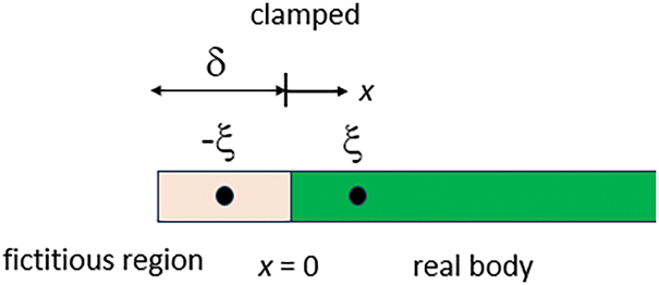
Figure A1: Introduction of the fictitious region for the clamped boundary condition

The PD governing equation for the boundary material point can be written as:

c∫−δδu(0+ξ)−u(0)|ξ|dξ=0(A1)

which can also be written as:

c∫0δu(0+ξ)−2u(0)+u(0−ξ)ξdξ=0⇒∫0δu(0+ξ)+u(0−ξ)ξdξ(A2)

(A2) is true for all horizon sizes, δ, and all deformation fields, u(x). Therefore, the following conditions must be satisfied:

u(−ξ)=−u(ξ)∀ξ∈[0,δ](A3)

Free Boundary

For a rod subjected to a free boundary at the right end (Fig. A2), a fictitious region can be introduced outside the free boundary with a width equal to the horizon size δ.

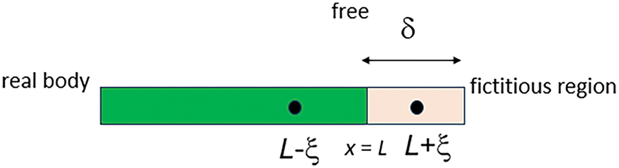
Figure A2: Introduction of the fictitious region for the free boundary condition

As a consequence of free boundary, it should be ensured that the resultant force acting on the real body from a fictitious region is zero. Let us denote f(x+η,x−ξ) as the bond force exerting on the material point located x−ξ from the material point located at x+η and it can be expressed as follows:

f(x+η,x−ξ):=cu(x+η)−u(x−ξ)|ξ+η|(A4)

Then, the following condition should hold:

∫0δ∫0δ−ξu(x+η)−u(x−ξ)|ξ+η|dηdξ=0  ⇔  ∫0δ∫0δ−ξf(x+η,x−ξ)dηdξ=0(A5a)

Alternatively, if the integral order is changed, the following expression can be obtained:

0=∫0δ∫0δ−ηu(x+η)−u(x−ξ)|ξ+η|dξdη=∫0δ∫0δ−ξu(x+ξ)−u(x−η)|η+ξ|dηdξ⇔0=∫0δ∫0δ−ηf(x+η,x−ξ)dξdη=∫0δ∫0δ−ξf(x+ξ,x−η)dηdξ(A5b)

By summing Eqs. (A5a) and (A5b) yields:

0=∫0δ∫0δ−ξf(x+ξ,x−η)dηdξ+∫0δ∫0δ−ξf(x+η,x−ξ)dηdξ=∫0δ∫0δ−ξ[f(x+ξ,x−η)+f(x+η,x−ξ)]dηdξ(A6)

Utilizing the mean value theorem:

∫0δ−ξ[f(x+ξ,x−η)+f(x+η,x−ξ)]dη=(δ−ξ)[f(x+ξ,x−α)+f(x+α,x−ξ)](A7)

For some α∈[0,δ−ξ], substituting Eq. (A7) into Eq. (A6) results in:

∫0δ(δ−ξ)[f(x+ξ,x−α)+f(x+α,x−ξ)]dξ=0(A8)

Again, if the mean value theorem is applied to Eq. (A8) yields:

∫0δ(δ−ξ)[f(x+ξ,x−α)+f(x+α,x−ξ)]dξ=δ(δ−β)[f(x+β,x−α)+f(x+α,x−β)]for some β∈[0,δ]=0(A9)

Eq. (A9) must be true for any arbitrary function f, which implies

f(x+β,x−α)+f(x+α,x−β)=0(A10)

and can be written as follows:

c[u(x+β)−u(x−α)|α+β|+u(x+α)−u(x−β)|α+β|]=[u(x+β)−u(x−β)]+[u(x+α)−u(x−α)]=0∀u(x)(A11)

Hence, it can be concluded that the following must hold for a free boundary condition:

u(L+ξ)=u(L−ξ)∀ ξ ε [0,δ](A12)

By assuming that the free boundary is located at x = L.

References

1. Silling SA. Reformulation of elasticity theory for discontinuities and long-range forces. J Mech Phys Solids. 2000;48(1):175–209. doi:10.1016/S0022-5096(99)00029-0. [Google Scholar] [CrossRef]

2. Silling SA, Epton M, Weckner O, Xu J, Askari E. Peridynamic states and constitutive modeling. J Elast. 2007;88(2):151–84. doi:10.1007/s10659-007-9125-1. [Google Scholar] [CrossRef]

3. Silling SA. Linearized theory of peridynamic states. J Elast. 2010;99(1):85–111. doi:10.1007/s10659-009-9234-0. [Google Scholar] [CrossRef]

4. Silling SA, Askari E. A meshfree method based on the peridynamic model of solid mechanics. Comput Struct. 2005;83(17–18):1526–35. doi:10.1016/j.compstruc.2004.11.026. [Google Scholar] [CrossRef]

5. Liu Y, Liu L, Mei H, Liu Q, Lai X. A modified rate-dependent peridynamic model with rotation effect for dynamic mechanical behavior of ceramic materials. Comput Meth Appl Mech Eng. 2022;388(24):114246. doi:10.1016/j.cma.2021.114246. [Google Scholar] [CrossRef]

6. Chen W, Gu X, Zhang Q, Xia X. A refined thermo-mechanical fully coupled peridynamics with application to concrete cracking. Eng Fract Mech. 2021;242(8):107463. doi:10.1016/j.engfracmech.2020.107463. [Google Scholar] [CrossRef]

7. Shi C, Zhang S, Zhang X, Li S. Peridynamics simulations of the damage of reinforced concrete structures under radial blasting. Int J Damage Mech. 2024;21(5):516. doi:10.1177/10567895241292745. [Google Scholar] [CrossRef]

8. Ma Q, Huang D, Wu L, Chen D. An improved peridynamic model for quasi-static and dynamic fracture and failure of reinforced concrete. Eng Fract Mech. 2023;289(2):109459. doi:10.1016/j.engfracmech.2023.109459. [Google Scholar] [CrossRef]

9. Wang Y, Wu W. A bond-level energy-based peridynamics for mixed-mode fracture in rocks. Comput Meth Appl Mech Eng. 2023;414(1):116169. doi:10.1016/j.cma.2023.116169. [Google Scholar] [CrossRef]

10. Wu WP, Li ZZ, Chu X. Peridynamics study on crack propagation and failure behavior in Ni/Ni3Al bi-material structure. Compos Struct. 2023;323:117453. doi:10.1016/j.compstruct.2023.117453. [Google Scholar] [CrossRef]

11. Chunyu GUO, Kang HAN, Chao WANG, Liyu YE, Zeping WANG. Numerical modelling of the dynamic ice-milling process and structural response of a propeller blade profile with state-based peridynamics. Ocean Eng. 2022;264(4):112457. doi:10.1016/j.oceaneng.2022.112457. [Google Scholar] [CrossRef]

12. Yang X, Gao W, Liu W, Li X, Li F. Peridynamics for out-of-plane damage analysis of composite laminates. Eng Comput. 2024;40(4):2101–25. doi:10.1007/s00366-023-01903-x. [Google Scholar] [CrossRef]

13. Oterkus E, Madenci E. Peridynamics for failure prediction in composites. In: 53rd AIAA/ASME/ASCE/AHS/ASC Structures, Structural Dynamics and Materials Conference 20th AIAA/ASME/AHS Adaptive Structures Conference; 2012 Apr 23–26; Honolulu, HI, USA. doi:10.2514/6.2012-1692. [Google Scholar] [CrossRef]

14. Oterkus E, Barut A, Madenci E. Damage growth prediction from loaded composite fastener holes by using peridynamic theory. In: 51st AIAA/ASME/ASCE/AHS/ASC Structures, Structural Dynamics, and Materials Conference; 2010 Apr 12–15; Orlando, FL, USA. doi:10.2514/6.2010-3026. [Google Scholar] [CrossRef]

15. Liu QQ, Wu D, Madenci E, Yu Y, Hu YL. State-Based peridynamics for thermomechanical modeling of fracture mechanisms in nuclear fuel pellets. Eng Fract Mech. 2022;276(16):108917. doi:10.1016/j.engfracmech.2022.108917. [Google Scholar] [CrossRef]

16. Jiang X, Fang G, Liu S, Wang B, Meng S. Fracture analysis of orthotropic functionally graded materials using element-based peridynamics. Eng Fract Mech. 2024;297(14–16):109886. doi:10.1016/j.engfracmech.2024.109886. [Google Scholar] [CrossRef]

17. Diana V, Bacigalupo A, Lepidi M, Gambarotta L. Anisotropic peridynamics for homogenized microstructured materials. Comput Meth Appl Mech Eng. 2022;392(1):114704. doi:10.1016/j.cma.2022.114704. [Google Scholar] [CrossRef]

18. Yin BB, Sun WK, Zhang Y, Liew KM. Modeling via peridynamics for large deformation and progressive fracture of hyperelastic materials. Comput Meth Appl Mech Eng. 2023;403:115739. doi:10.1016/j.cma.2022.115739. [Google Scholar] [CrossRef]

19. O’Grady J, Foster J. Peridynamic beams: a non-ordinary, state-based model. Int J Solids Struct. 2014;51(18):3177–83. doi:10.1016/j.ijsolstr.2014.05.014. [Google Scholar] [CrossRef]

20. Liu S, Fang G, Liang J, Fu M, Wang B, Yan X. Study of three-dimensional Euler-Bernoulli beam structures using element-based peridynamic model. Eur J Mech A/solids. 2021;86(9):104186. doi:10.1016/j.euromechsol.2020.104186. [Google Scholar] [CrossRef]

21. Chen Y, Yang Y, Liu Y. Fatigue crack growth analysis of hydrogel by using peridynamics. Int J Fract. 2023;244(1):113–23. doi:10.1007/s10704-023-00722-x. [Google Scholar] [CrossRef]

22. Wang Y, Zhou X, Wang Y, Shou Y. A 3-D conjugated bond-pair-based peridynamic formulation for initiation and propagation of cracks in brittle solids. Int J Solids Struct. 2018;134(1-2):89–115. doi:10.1016/j.ijsolstr.2017.10.022. [Google Scholar] [CrossRef]

23. Zu L, Liu Y, Zhang H, Liu L, Lai X, Mei H. An elastoplastic fracture model based on bond-based peridynamics. Comput Model Eng Sci. 2024;140(3):2349–71. doi:10.32604/cmes.2024.050488. [Google Scholar] [CrossRef]

24. Liu Z, Zhang J, Zhang H, Ye H, Zhang H, Zheng Y. Time-discontinuous state-based peridynamics for elasto-plastic dynamic fracture problems. Eng Fract Mech. 2022;266(3):108392. doi:10.1016/j.engfracmech.2022.108392. [Google Scholar] [CrossRef]

25. Tian DL, Zhou XP. A viscoelastic model of geometry-constraint-based non-ordinary state-based peridynamics with progressive damage. Comput Mech. 2022;69(6):1413–41. doi:10.1007/s00466-022-02148-z. [Google Scholar] [CrossRef]

26. Zhang J, Yang QS, Liu X. Peridynamics methodology for elasto-viscoplastic ductile fracture. Eng Fract Mech. 2023;277(5):108939. doi:10.1016/j.engfracmech.2022.108939. [Google Scholar] [CrossRef]

27. Zhang T, Zhou XP, Qian QH. Drucker-Prager plasticity model in the framework of OSB-PD theory with shear deformation. Eng Comput. 2023;39(2):1395–414. doi:10.1007/s00366-021-01527-z. [Google Scholar] [CrossRef]

28. Oterkus E, Madenci E, Nemeth M. Stress analysis of composite cylindrical shells with an elliptical cutout. J Mech Mater Struct. 2007;2(4):695–727. doi:10.2140/jomms.2007.2.695. [Google Scholar] [CrossRef]

29. Mikata Y. Analytical solutions of peristatic and peridynamic problems for a 1D infinite rod. Int J Solids Struct. 2012;49(21):2887–97. doi:10.1016/j.ijsolstr.2012.02.012. [Google Scholar] [CrossRef]

30. Mikata Y. Analytical solutions of peristatics and peridynamics for 3D isotropic materials. Eur J Mech A/solids. 2023;101(6):104978. doi:10.1016/j.euromechsol.2023.104978. [Google Scholar] [CrossRef]

31. Yang Z, Ma CC, Oterkus E, Oterkus S, Naumenko K. Analytical solution of 1-dimensional peridynamic equation of motion. J Peridyn Nonlocal Model. 2023;5(3):356–74. doi:10.1007/s42102-022-00086-1. [Google Scholar] [CrossRef]

32. Yang Z, Ma CC, Oterkus E, Oterkus S, Naumenko K, Vazic B. Analytical solution of the peridynamic equation of motion for a 2-dimensional rectangular membrane. J Peridyn Nonlocal Model. 2023;5(3):375–91. doi:10.1007/s42102-022-00090-5. [Google Scholar] [CrossRef]

33. Wang B, Oterkus S, Oterkus E. Determination of horizon size in state-based peridynamics. Continuum Mech Thermodyn. 2023;35(3):705–28. doi:10.1007/s00161-020-00896-y. [Google Scholar] [CrossRef]

34. Oterkus S, Oterkus E. Comparison of peridynamics and lattice dynamics wave dispersion relationships. J Peridyn Nonlocal Model. 2023;5(4):461–71. doi:10.1007/s42102-022-00087-0. [Google Scholar] [CrossRef]