Developed Time-Optimal Model Predictive Static Programming Method with Fish Swarm Optimization for Near-Space Vehicle

1  Introduction

Research on near-space vehicles has recently become a hot topic in the aerospace field [1], with the success of such missions heavily relying on their effective guidance, navigation, and control systems [2]. The performance of these systems is critical to the success of the entire flight [3], as failures can result in catastrophic consequences. Consequently, developing an effective guidance method is essential for near-space vehicles. Current guidance methods can meet terminal angle [4] and position [5] constraints; however, the feedback-based methods fail to address other important requirements, such as constraints on terminal velocity and the need for minimal fuel consumption. During the glide phase, it is important to design an optimal trajectory that satisfies every constraint. Some scholars proposed various tracking methods [6] to control terminal states by optimal reference trajectory [7,8]. The reference trajectory is open-loop, with a closed-loop tracking controller employed to follow it. This paper focuses on designing an optimal reference trajectory [9] that can be rapidly and accurately generated for the near-space vehicle. Recently, many scholars have conducted in-depth research on trajectory optimization problems [10,11]. In the aerospace field, Chai et al. [12] reviewed outstanding developments in numerical multi-objective trajectory programming methods. Malyuta et al. [3] provided an overview of recent advances and successes in optimization-based space vehicle control problems, offering promising directions for future research. Li et al. [13] systematically summarized and reviewed various optimization methods from both global and Chinese competitions, proposing development trends and promising solutions for trajectory programming challenges. Shirazi et al. [14] outlined the steps involved in spacecraft trajectory optimization problems. The current trajectory optimization methods are primarily classified into direct methods and indirect methods [15]. On the one hand, the indirect method using Lagrange multipliers transforms the optimal control problem into a two-point boundary value problem, and solves it via minimum principle [16,17]. To explore the impact of electrical power constraints on the gradients in trajectory programming, Wang et al. [18] employed a high-efficiency indirect method. Under the condition of free terminal time, Nakano et al. [19] proposed an indirect method to address the asteroid landing trajectory programming problem with the objective of minimizing fuel consumption. In addressing the trajectory optimization problem for an Unmanned Aerial Vehicle (UAV), Coupechoux et al. [20] using Lagrangian mechanics and Hamilton-Jacobi equations established a closed-form optimal trajectory. In summary, while the indirect method ensures high accuracy and optimality for trajectory optimization through the first-order necessary condition, problems such as a small convergence radius and sensitivity to initial values limit its applicability for real-time trajectory optimization in aerospace applications. On the other hand, the direct method solves the optimal control problem by discrete nonlinear dynamic equations and nonlinear programming (NLP). For direct trajectory programming of a free-floating space manipulator, Shao et al. [21] enhanced the current nonlinear programming method by an adaptive Radau Pseudospectrum technique. Methods that do not require costate calculation can be classified as direct methods. For high-precision trajectory optimization of the Dreyfus rocket and inverted pendulum, Sun et al. [22] proposed two novel differential dynamic programming methods. Ma et al. [23] developed a sequential convex programming method for the launch vehicles in the ascent stage, employing an enhanced Chebyshev-Picard iteration. To reduce the computational burden of real-time trajectory programming for UAV, Xu et al. [24] proposed a trust-region-constrained sequential convex programming method. Chapnevis et al. [25] utilized integer linear programming to solve the multi-target UAV trajectory optimization problem. In summary, the direct method offers three advantages over the indirect method: 1) low computational complexity; 2) high computational efficiency; and 3) large convergence radius. Motivated by the advantages of the direct method, some scholars proposed model predictive static programming (MPSP) to achieve fast and high-precision trajectory optimization. Padhi et al. [26] first proposed the MPSP method by combining approximate dynamic programming and model predictive control. To design the missile’s optimal trajectory, Fu et al. [27] introduced slack variables for state inequality constraints and enhanced the current MPSP method. For the optimal trajectory design of satellites, Wang et al. [28] using a two-loop MPSP guidance scheme established fuel-optimal trajectories as nominal solutions. For interceptors targeting incoming ballistic missiles, Dwivedi et al. [29] using MPSP proposed two nonlinear suboptimal midcourse guidance methods. Zhou et al. [30] using Gaussian quadrature collocation proposed a novel generalized quasi-spectral MPSP method. Pan et al. [31] demonstrated that the MPSP method is an improved Newton-type trajectory optimization method. Although the above methods have relatively good simulation effects, there is still some room for improvement in two aspects: 1) the improvement of optimization accuracy and speed. The above methods do not pay much attention on how to improve the accuracy and speed of the current model predictive static programming method. In general, accuracy and speed are very important for online trajectory optimization. Thus, it is essential to study how to speed up the method’s solving accuracy and speed. 2) the trajectory optimization problem under free terminal time. In typical aerospace missions, the final flight time is not a primary concern. Compared to the fixed time trajectory optimization problem, the performance index (fitness function) of the generated trajectory is lower when the time is flexible. Consequently, it is necessary to study the problem under free terminal time to gain an optimal performance index. Linearization theory is employed in the current method to obtain optimal flight time in MPSP [32]. The Taylor expansion may lead to lower solving accuracy which will sacrifice performance index and degrade flight performance. To improve the accuracy, some scholars employed intelligent methods: Zamfirache et al. [33] developed a Grey Wolf Optimizer (GWO) method to train Neural Networks in the reinforcement learning-based control method. To enhance the conventional GWO method’s accuracy, Zamfirache et al. [34] further proposed a gravitational search method to initialize the Q-function’s parameter which has better results in reinforcement learning. Additionally, some scholars developed the fish swarm optimization method for high-precision, complex trajectory optimization problems. For example, Tsai et al. [35] proposed a particle swarm optimization framework to improve the existing fish swarm optimization method. Sivakumar et al. [36] developed the current fish swarm optimization method to minimize the sensor node position errors. To more effectively address the drone path programming problem, Zhang et al. [37] developed the current artificial fish swarm optimization method. To address the problem of Unmanned Helicopter formations, Ma et al. [38] proposed a path planning method based on the developed artificial fish swarm optimization method, considering both neighborhood learning and method characteristics. The above intelligent methods have the following problems: 1) it is easy to fall into the local optimal solution (sub-optimal solution); 2) The fixed step will affect the solving speed for complex optimization problems. Motivated by the preceding discussions, a developed time-optimal model predictive static programming (D-MPSP) method is proposed for near-space vehicle with adaptive fish swarm optimization and momentum gradient descent (AFSO-MGD). Note that this method is also applicable to a wide range of aerospace problems that require trajectory optimization. In this method, the D-MPSP method with a neighboring term and trust region is proposed to determine the optimal flight trajectory that satisfies the terminal state constraints under fixed terminal time. Additionally, when the terminal time is free, the AFSO-MGD method is employed to optimize terminal time to minimize performance index (fitness function). In this method, the fish swarm optimization is employed to explore the sub-optimal solution, while the momentum gradient descent focuses on finding the global optimal solution. Compared to previous research on trajectory optimization, the primary contributions of this paper can be summarized as follows: 1) Compared to the current method, a developed model predictive static programming method with neighboring term and trust region is proposed to enhance both the speed and accuracy of trajectory optimization. The trust region guarantees the solution’s accuracy and efficiency, while the neighboring term guarantees that the updated solution remains within the neighborhood of the reference trajectory, thus ensuring that the solution process stays within in the convergence radius. 2) Compared to the conventional method under free terminal time, the adaptive fish swarm optimization method with momentum gradient descent significantly improves the solution accuracy, while avoiding the current method’s linearization errors caused by analytical derivations. Then the adaptive theory facilitates rapid convergence. Meanwhile, the momentum gradient descent method prevents the solution from being trapped in a local optimum.

The rest of this paper is organized as follows. In Section 2, the dynamic model is established for near-space vehicle, then Euler method is employed for discretization. In Section 3, the main contributions of this paper are presented, the detailed theory about time-optimal model predictive static programming method is proposed with adaptive fish swarm optimization. In Section 4, a numerical example for near-space vehicle is implemented to verify the proposed method’s feasibility. In Section 5, the compared methods are implemented to demonstrate the proposed method’s accuracy. Finally, some conclusions are drawn in Section 6.

2  Dynamic Model for Near-Space Vehicle

The near-space vehicle’s dynamic equation [39] is obtained in Eq. (1):

{x˙=υcos⁡γcos⁡ψy˙=υsin⁡γz˙=−υcos⁡γsin⁡ψv˙=g(nx−sin⁡γ)θ˙=gv(ny−cos⁡γ)ψ˙=−gnzυcos⁡γ(1)

where, state quantities are downrange, altitude, lateral position, flight-path angle and heading angle, respectively; nx, ny and nz are three-shaft overloads, respectively; ny and nz are optimized variables; nx is given by:

nx=−ρυ2CDS2mg(2)

in which, S is reference area (S=0.5 m2); g is gravitational acceleration (g=9.81 m/s2); ρ is density:

ρ=1.225exp⁡(−y7110)(3)

Euler method is employed to discrete Eq. (1):

{xk+1=xk+[υkcos⁡γkcos⁡ψk]dtyk+1=yk+[υksin⁡γk]dtzk+1=zk+[−υkcos⁡γksin⁡ψk]dtυk+1=υk+[g(nxk−sin⁡γk)]dtθk+1=θk+[gυk(nyk−cos⁡γk)]dtψk+1=ψk+[−gnzkυkcos⁡γk]dt(4)

in which, dt is the step.

3  Developed Time-Optimal Model Predictive Static Programming Method

In this section, the time-optimal model predictive static programming method is proposed with neighboring term and trust region for rapid and precise trajectory optimization. In addition, the adaptive fish swarm optimization is developed for model predictive static programming method under free terminal time.

3.1 Model Predictive Static Programming with Neighboring Term and Trust Region

The model predictive static programming method is to establish the optimal trajectory satisfying terminal state constraints. Eq. (4) can be simplified as:

Xk+1=Gk(Xk,Uk)(5)

where, k is the iterative number; state vector is Xk=[xkykzkυkγkψk]T and control vector is Uk=[nyknzk]T. The output equation is:

Zk=Xk(6)

in which, Zk is output state vector (observed state vector). Linearizing Eq. (5) in the neighboring area of reference trajectory, one has:

δXk+1=∂Gk∂XkδXk+∂Gk∂UkδUk(7)

where, δXk is the deviation of Xk, ∂Gk∂Uk and ∂Gk∂Xk are partial derivatives with respect to U and X, respectively.

According to Eq. (7), one has:

δZf=δXf=∂Gf−1∂Xf−1δXf−1+∂Gf−1∂Uf−1δUf−1(8)

By Eqs. (7), (8) is changed as:

δZf=∂Gf−1∂Xf−1(∂Gf−2∂Xf−2δXf−2+∂Gf−2∂Uf−2δUf−2)+∂Gf−1∂Uf−1δUf−1(9)

By induction from Xf to X1, one has:

δZf=AδX1+∑i=1f−1BiδUi(10)

in which, i is discrete time step (i = 1, 2, … , f-1); matrices A and Bi are given by:

A=[∂Gf−1∂Xf−1][∂Gf−2∂Xf−2]⋯[∂G2∂X2][∂G1∂X1](11)

Bi=[∂Gf−1∂Xf−1][∂Gf−2∂Xf−2]⋯[∂Gi+2∂Xi+2][∂Gi+1∂Xi+1][∂Gi∂Ui](12)

It is not necessary to consider the initial state perturbations for near-space vehicle in trajectory optimization problem, thus Eq. (10) is reduced to:

δZf=∑i=1f−1BiδUi(13)

The control curves’ design needs to ensure the smoothness as much as possible, given the limitations of near-space vehicle’s control capability. Therefore, the continuous system’s performance index Jc is designed as:

Jc=12∫t0tf(UTRU)dt(14)

where, R is the user-designed control weight matrix; t0 and tf are initial and terminal times, respectively. The performance index designed in Eq. (14) guarantees the smooth control curves which have two advantages: 1) The smooth reference trajectory guarantees that the subsequent attitude control system has a large control margin; 2) The smooth curves significantly reduce the demands on both the steering mechanism and the structure of near-space vehicle.

Discretize Eq. (14):

Jd=12∑i=1f−1UiTRUi(15)

To improve terminal state control accuracy and guarantee optimal performance index, multiple iterations are implemented. The performance index Jd is changed as J:

J=12∑i=1f−1(Uir−δUir)TR(Uir−δUir)+(−δUir)TKδu(−δUir)(16)

where, Uir is the control history calculated by reference trajectory; δUir is the deviation control history; Kδu is the penalty coefficient of error term. Note that, U and δU should have different signs in Eq. (16). If they have different signs:

∂J∂U>0,∂J∂δU<0→{1) J↘,U↘,δU↗2) J↗,U↗,δU↘ ⇒trajectory convergence(17)

In condition 1), with J decreasing, control U decreases while δU increases; In condition 2), with J increasing, control U increases while δU decreases. The above analysis ensures the trajectory convergence through multiple iterations.

The quadratic error term designed in Eq. (16) is regarded as a trust region. Its advantages are shown as follows: 1) It improves the optimization accuracy, and subsequent simulations demonstrate a significant improvement in accuracy; 2) It ensures the proximity of the trajectories in two iterations, guaranteeing that the final solution converges within the feasible region; 3) It reduces the iterative number and enhances efficiency, which is important for real-time trajectory optimization of near-space vehicle. Now the optimal MPSP problem is established. To address this problem, the optimal control theory is employed through the Lagrange multiplier method [40]. The augmented performance index J¯ is given by:

J¯=12∑i=1f−1(Uir−δUir)TR(Uir−δUir)+(−δUir)TKδu(−δUir)+λT(δZf−∑i=1f−1BirδUir)(18)

where, λ is the Lagrange multiplier vector.

Assuming no control constraint, the optimal necessary condition is given by:

∂J¯∂δUir=−R(Uir−δUir)−Kδu(−δUir)+BirTλi=0(19)

Control perturbation δUir is obtained by Eq. (20):

δUir=(R+Kδu)−1(RUir−BirTλi)(20)

Now the essential problem is to solve Lagrange multiplier vector in Eq. (20):

δZf=∑i=1f−1Bir(R+Kδu)−1(RUir−BirTλi)=∑i=1f−1Bir(R+Kδu)−1RUir−Bir(R+Kffiu)−1BirTλi(21)

By Eq. (21), Lagrange multiplier vector is obtained by a simple inversion:

λi=−(∑i=1f−1Bir(R+Kδu)−1BirT)−1(δZf−∑i=1f−1Bir(R+Kδu)−1RUir)(22)

Combining Eqs. (20) and (22):

δUir=(R+Kδu)−1{RUir+BirT[∑i=1f−1Bir(R+Kffiu)−1BirT]−1[δZf−∑i=1f−1Bir(R+Kδu)−1RUir]}(23)

Then the updated control law is obtained in Eq. (24):

Ui=Uir−δUir(24)

where, Ui is the updated control history. Eq. (24) is the iterative equation of model predictive static programming method with trust region.

Then the neighboring term is implemented to ensure that the proposed method is solved in the feasible region, given that the control constraint is not considered in Eq. (19). With the updated control history, the state deviations are calculated by integrating the dynamic equations:

δXi=∑i=1f−1Xi−Xir(25)

where, Xi, Xir and δXi represents updated state vector, reference state vector, and state deviation vector, respectively.

Then the performance index F based on state deviations is established in Eq. (26):

F=δx^Kδxδx^+δy^Kδyδy^+δz^Kδzδz^+δv^Kδvδv^+δγ^Kδγδγ^+δψ^Kδψδψ^(26)

in which, K represents the normalized penalty coefficient for corresponding state deviations; then one has:

x^=xxmax,y^=yymax,z^=zzmax,v^=vvmax,γ^=γγmax,ψ^=ψψmax(27)

in which, “max” represents the maximum value of state in reference trajectory.

A neighboring term based on state deviations in Eq. (26) is established as:

F<Fmax(28)

where, Fmax represents the maximum value of objective function. In Eq. (28), if this condition is satisfied, the proposed method continues to execute; otherwise, the following method is applied to ensure that the solution remains within the feasible region:

δUir=(Ktrust)mδUir(29)

in which, Ktrust is a positive number and less than 1, m is the iterative number of neighboring term.

The pseudocode is shown in Table 1:

3.2 Adaptive Fish Swarm Optimization Method with MGD under Free Terminal Time

Most trajectory optimization problems are more sensitive to performance index rather than to terminal time, making it essential to study the problem under free terminal time. The current fish swarm optimization method suffers from slow convergence and a tendency to get trapped in local optimum. To solve this problem, the adaptive theory [41,42] and momentum gradient descent method with learning rate decay are employed. Before optimization, the fish swarm size, the maximum number of tries (try number), crowding parameter (delta), the maximum iterative number (maxgenf), and the visual distance (visual) should be set. Through sensitivity analysis and multiple simulation verifications, it was found that the fish swarm size and the maximum iterative number have significant impacts on computational complexity. To balance computational complexity and optimization accuracy, the fish swarm size and maximum iterative number are both determined to be 3 by using the additional optimization method. To further improve the iterative efficiency, the adaptive step is employed. In this method, the initial larger step ensures the convergence of the proposed method, and the later smaller step ensures sub-optimal results. The adaptive step is obtained as:

stepi+1=Kstepgen|bestJ|(30)

where, gen is the current iterative number; bestJ is the global optimal solution for current iteration; Kstep is the parameter to set. The adaptive fish swarm optimization method consists of four main parts. In the foraging part, the flow is:

In Fig. 1, subscript m represents the random individual in sight line, the subscript i represents different individual fish; ti is the current time of individual fish; rand is the random number range from −1 to 1; k is the current try number; J is the fitness function (performance index) to be optimized, the same as that in Eq. (15). For the minimization optimization problem, if Ji > Jm, enter foraging behavior; otherwise, determine whether to enter random mode or iterate again.

Figure 1: Foraging behavior flowchart

In the gathering and following part, the flow is:

In Fig. 2, dij is the second norm of distance between individual fishes, δ is the crowding parameter to set, nf is the number of partners in the neighborhood, c represents the central location of the partners. If (Jc/nf) < δJi, enter gather behavior; else, enter foraging behavior; if (Jj/nf) < δJi, enter follow behavior; else, enter foraging behavior.

Figure 2: Gather and follow behavior flowchart

In random part, individual fish randomly select a state within its visible range:

ti−update=ti+rand⋅visual(31)

The above four parts are the core of the adaptive fish swarm optimization method. In this method, strategies to prevent overfitting can be implemented from the following seven aspects: 1) Enhancing population diversity: by periodically introducing random perturbations to some individuals or adding new random individuals, population diversity is maintained to avoid premature convergence to local optima; 2) Adaptive parameter adjustment: dynamically adjust parameters (step or search range) based on the iterative number, gradually narrowing the search space or optimizing step to prevent the proposed method from getting stuck in local optima; 3) Regularization methods: incorporate penalty terms related to solution complexity into the fitness function to suppress overly complex solutions, thereby reducing the risk of overfitting; 4) Cross validation: divide the dataset into training and validation sets, run multiple times, and select the best solution on the validation set to ensure the model’s generalization capability; 5) Early stopping strategy: continuously monitor the fitness function on the validation set. If no improvement is observed after several iterations, terminate the method early to avoid overfitting the training data; 6) Ensemble methods: run the fish swarm optimization method multiple times and integrate the results (voting or weighted averaging) to reduce the risk of overfitting by combining the outputs of multiple models; 7) Constraining the search space: impose reasonable constraints on the solution space based on the problem’s practical context, preventing the method from searching in overly complex or irrelevant regions. By implementing the above strategies, the risk of overfitting in adaptive fish swarm optimization methods can be effectively mitigated, significantly enhancing the method’s generalization ability and robustness. However, the problem of the current method will converge at suboptimal solutions rather than optimal solutions for nonlinear and coupled problems. To resolve this problem, the momentum gradient descent method is employed. Gradient descent is developed based on exponential weighted average, and its equation for k iteration is:

vk=βvk−1+(1−β)∇f(tk)(32)

where, ∇f represents the gradient value, β represents weight coefficient, vk−1 is updated weighted gradient value. Due to the exponential weighted average, the direction of parameter update is not only affected by the current gradient, but also by the previous gradient, making the parameter update path smoother. To address the problem of poor convergence in the above method due to large learning rate, a learning rate decay method is employed as:

hupdate=h+∇f(tk)⋅∇f(tk)(33)

in which, h represents the sum of squared gradient values. Combining the above two methods, the final iteration update rule is given by:

xk+1=xk−Kmvk−η1h∇f(tk)(34)

where, Km is the parameter to set, and η is the learning rate. Note that the learning rate itself is dynamically adjusted by updated weight coefficient h.

This proposed method consists of two parts: fish swarm optimal method for sub-optimal solution and momentum gradient descent method for global optimal solution.

3.3 Method Flow

Fig. 3 shows the design flowchart for the whole method in detail.

Figure 3: Method flow

Fig. 3 shows that the model predictive static programming method is employed to generate an optimal reference trajectory that satisfies the initial and terminal state constraints under fixed terminal time. The adaptive fish swarm optimization method is aimed at looking for the sub-optimal solution, while the gradient descent method is implemented to generate a global optimal solution. Note that, the proposed method is used not only to the near-space vehicle, but also to all kinds of aerospace problems that require trajectory optimization. Additionally, the computational complexity of this proposed method is discussed. 1) For the model predictive static programming method with trust region and neighboring term, a symbolic recursive solution to directly update control history makes it suitable for trajectory optimization in online guidance systems. Therefore, the key factor influencing its solving speed lies in the number of discrete points and the quality of the initial values (initial control history guess). 2) For the adaptive fish swarm optimization and momentum gradient descent methods, their computational complexity primarily depends on the fish swarm size and the maximum iterative number. For time-sensitive trajectory optimization problems, these parameters need to be carefully set to ensure the online trajectory optimization capability for computational guidance. Finally, the hardware implementation is discussed. The hardware requirements for this real-time guidance system depend on factors such as the application’s complexity, speed, and operating environment. It is important to note that the proposed method does not require high computational resources. Consequently, it is not necessary to use expensive, high-performance hardware. Given the cost constraints for large-scale deployment, the proposed method proves to be highly practical. Additionally, this method does not rely on complex toolboxes and can be easily converted into a C++ program for deployment on a near-space vehicle’s micro-controller. As a result, the implementation of the proposed method is relatively straightforward from software to hardware.

4  Case Study: Time-Optimal Model Predictive Static Programming Method for Near-Space Vehicle

In this section, the simulation of the near-space vehicle example is implemented. First, the simulation results of the proposed model predictive static programming method with neighboring terms and trust region are presented. Next, the proposed adaptive fish swarm optimization method is validated under free terminal time. Finally, the tracking accuracy of terminal controllers is demonstrated with an optimal reference trajectory. The initial and terminal state constraints are set in Table 2.

4.1 Model Predictive Static Programming with Neighboring Term and Trust Region

This section uses neighboring term and trust region for current model predictive static programming method. Other parameters are set as: terminal time (tf): 44.5 s, R = [1 0; 0 1], and Kδu = diag (10, 10). Shown in Figs. 4–10 are the simulation results in 8 iterations.

Figure 4: Iterations of three-dimensional trajectories

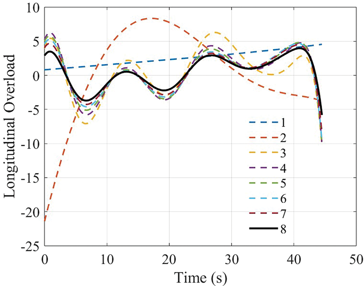
Figure 5: Iterations of longitudinal overload profiles

Figure 6: Iterations of lateral overload profiles

Figure 7: Iterations of flight-path angle profiles

Figure 8: Iterations of heading angle profiles

Figure 9: Iterations of velocity profiles

Figure 10: Iterations of performance index profiles

Figs. 4–10 show that every state achieves good convergence through 8 iterations. In particular, good convergence is achieved for the relatively sensitive terminal velocity. Given the influence of nonlinearity and coupling in dynamic equations, the proposed model predictive static programming method with a neighboring term and trust region has high convergence efficiency and good convergence accuracy. These results will be further explained later in Section 5.2. Then the 500 Monte Carlo simulations are presented in Figs. 11 and 12. In this simulation, based on the initial states’ reference values in Table 2, the perturbation ranges of the initial downrange, altitude, and lateral position are [–500 500] m, while the perturbation ranges of the initial flight-path and heading angles are [−1 1] deg.

Figure 11: Monte Carlo of 3D trajectory profiles

Figure 12: Monte Carlo of velocity profiles

Under the different initial state perturbations, Fig. 11 demonstrates that each trajectory achieves high-precision convergence, especially sensitive terminal velocity in Fig. 12. Consequently, it proves the proposed method’s robustness.

Next, the convex optimization method and GPOPS (a matlab software for solving multiple-phase optimal control problems) trajectory optimization method is compared to verify the effectiveness and accuracy of the proposed method. Convex optimization is a widely used trajectory optimization method. It has advantages such as a well-defined convergence criterion and relatively high solution efficiency. However, the constraints in trajectory optimization problems are typically non-convex, requiring the original problem to be transformed into a convex one by sequential convexification or lossless convexification. The sequential convex optimization method requires converting the original problem into a standard form required by specific toolboxes and solving large-scale nonlinear programming problems, which increases the computational complexity of engineering implementation. In contrast, the proposed method updates the deviation control history through a Lagrange multiplier with a symbolic recursive solution, and then combines it with the reference control history to indirectly update the control history. This method achieves higher computational efficiency and lower computational complexity. Then the GPOPS trajectory optimization method is generally considered an offline trajectory optimization method, as its nonlinear programming method consumes substantial computational resources. Using MATLAB numerical simulation software, the simulation results show that the trajectory optimization time (CPU time) for GPOPS is 4 s, for convex optimization is 1.8 s, and for the proposed model predictive static programming method is less than 1 s. This demonstrates that the proposed method offers higher optimization efficiency.

4.2 Model Predictive Static Programming under Free Terminal Time

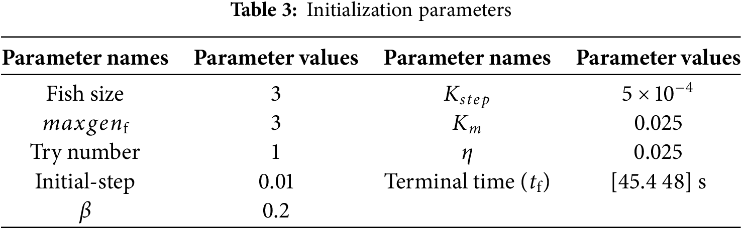
In this section, the model predictive static programming method is implemented under free terminal time. The initial flight time is set to 44.3 s. Parameters are initialed in Table 3.

The fitness function curve is presented in Fig. 13.

Figure 13: Curve of performance index (fitness function) with iterative number

With the increase of iteration times, the fitness function gradually decreases in Fig. 13. Note that, the fitness function does not converge completely, because the proposed adaptive fish swarm optimization method guarantees global convergence over a large range to obtain the suboptimal solution rather than the optimal one. To obtain the optimal solution, the momentum gradient descent method is employed. In Fig. 13, the sub-optimal performance index J = 196.6544 while tf = 45.50 s. After the adaptive fish swarm optimization method, the momentum gradient descent method is employed. The best solution (global optimal solution) is J = 196.6514 while tf = 45.51 s. The reduction in performance index ensures smooth control curves, which is beneficial for the attitude tracking system.

4.3 Terminal Controllers for Tracking Guidance Based on Reference Trajectory

Given that the trajectory designed above is open-loop, a closed-loop guidance method is employed to track it. A current terminal controller is presented to track reference trajectory due to their general applications treated and relation to this paper. The detailed theory and equation derivation can be seen in [6]. The optimal terminal controller can be given in Eqs. (35)–(37):

X=XREFERENCE+δX(35)

δU=−R−1DTSδX(36)

U=UREFERENCE+δU(37)

in which, R is the control weight matrix; D is the control partial derivative matrix; S is the feedback matrix by backward integration; “REFERENCE” represents reference trajectory.

In this simulation, “TRACK1” denotes the tracking trajectory without any perturbation in wind speed and gravitational acceleration; “TRACK2” indicates the tracking trajectory affected by gravitational acceleration perturbation, with a range of −1 to 1; “TRACK3” indicates the tracking trajectory with wind speed perturbation, with a range of −5 to 5; “TRACK4” presents the tracking trajectory impacted by both gravitational acceleration and wind speed perturbations, with perturbation ranges matching those of “TRACK3” and “TRACK4”. The initial state perturbations are provided in Table 4 for simulations “TRACK1” to “TRACK4”. And the simulation results are presented in Table 4 and Figs. 14–18.

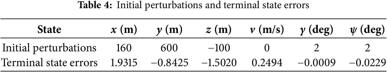
Figure 14: Trajectory tracking curves

Figure 15: Longitudinal overload tracking curves

Figure 16: Lateral overload tracking curves

Figure 17: Flight-path angle tracking curves

Figure 18: Heading angle tracking curves

Under larger initial state perturbations, Table 4 and Figs. 14–18 demonstrate the terminal position, velocity and angle errors remain small compared to the reference trajectory. All state and control curves quickly converge to the reference values, indicating that the controller exhibits strong tracking performance and precision. It is important to emphasize that various disturbances in actual flight, such as initial perturbations and model uncertainties, may lead to deviations of near-space vehicles from their reference trajectory. The closed-loop control strategy employed in this study ensures high-precision convergence of terminal states.

5  Method Comparison

In this section, two method comparisons are presented. First, the proposed adaptive fish swarm optimization method is compared with the current analysis method for solving free-time trajectory optimization problems. Secondly, a comparative evaluation is conducted between the proposed methods with and without the neighboring term and trust-region.

5.1 Method Comparison between Proposed and Current Methods under Free Terminal Time

To verify the simulation results of trajectory optimization methods under free terminal time, proposed and current methods are compared. The current methods are briefly presented as follows and the detailed theory can be seen in [32].

Different from the performance index in current model predictive static programming method, the developed performance index Jfree in time-free problem is given by:

Jfree=12cf(dtf)2+12∑i=1f−1(Uir−dUir)TR(Uir−dUir)(38)

where, R is the control weight matrix; cf is the weight term for terminal time deviation (dtf).

The terminal state deviation is given by:

dZf=∑i=1f−1BidUi+∂Zf∂Xff(Xf,Uf)dtf(39)

in which, matrices f and Bi are the same as those in Eqs. (1) and (10), respectively.

The first-order optimal necessary conditions are changed as:

∂J¯free∂dUir=−R(Uir−dUir)−BirTλi=0(40)

∂J¯free∂dtf=cf(dtf)−{[∂Zf∂Xf]f(Xf,Uf)}Tλ=0(41)

Then the control history and terminal time are updated as:

uk−update=Rk−1{[BkT(Aλ+Cλ)−1(−dZf+bλ)]}(42)

tf−update=tfref+cf−1{[∂Zf∂Xf]f(Xf,Uf)}T(Aλ+Cλ)−1(−dZf+bλ)(43)

where, Aλ, bλ and Cλ are the parameter matrices; uk-update and tf-update represent the updated u and tf, respectively.

Given that the current method does not impose constraints on the neighboring term and trust region, this comparison only focuses on the time-free trajectory optimization problem. In the simulation, “Proposed” represents the proposed method, while “Analysis” denotes the current analytic terminal time estimation method. The parameter cf is set to 106. Figs. 19–24 demonstrate the comparison results.

Figure 19: Three-dimensional trajectory profiles

Figure 20: Performance index profiles

Figure 21: Longitudinal overload profiles

Figure 22: Lateral overload profiles

Figure 23: Flight-path angle profiles

Figure 24: Heading angle profiles

Figs. 19–24 show both methods achieve fast convergence of trajectories. It is obvious that the proposed method has smoother curves and better simulation results. Additionally, the smooth trajectories are beneficial for the subsequent attitude control system. The data statistics for terminal time estimation are presented and compared in Table 5.

The comparative results presented in Table 5 indicate that the proposed method achieves a substantially lower performance index than that in the analytic method, confirming the proposed method’s effectiveness.

5.2 Method Comparison between Whether Implementing Trust Region

In this subsection, the iterative number is set to 7; the terminal flight time is set to 44.5 s; and Kδu = diag(10,10). These simulation results comparing the method with and without the neighboring term are presented in Table 6. The method “With constraint” presents the proposed model predictive static programming method with trust region in Section 3, while the method “Without constraint” represents the current model predictive static programming method.

Table 6 presents the error terms, which represent the differences between the desired and actual terminal states. Compared to the current method, which does not incorporate trust region, the proposed method significantly reduces terminal state errors. The improved precision offers several advantages: 1) It further enhances the trajectory optimization capability of near-space vehicle during the glide phase; 2) It reduces the number of discrete points required to complete the trajectory optimization task, thereby significantly decreasing optimization time; 3) It ensures smooth state and control curves between two adjacent iterations; 4) A key advantage of the model predictive static programming method with trust region is that this constraint ensures iterative smoothness and minimize terminal state errors.

6  Conclusion

In this paper, firstly, the model predictive static programming method is proposed with a neighboring term and trust region. Secondly, to address the free terminal time problem, an adaptive fish swarm optimization method is developed to optimize terminal flight time to obtain a sub-optimal solution, while the momentum gradient descent method with a decaying learning rate is employed to achieve the global optimal solution. The final conclusions are drawn as: 1) The designed neighboring term and trust region for the current model predictive static programming method significantly improve solution accuracy, reduce solving time to some extent, and guarantee smooth optimal solutions; 2) The adaptive fish swarm optimization and momentum gradient descent methods ensure the global optimal solution in model predictive static programming method under free terminal time. The global optimal solution reduces energy consumption and ensures a smooth trajectory for near-space vehicles, which greatly benefits their structural and rudder surface design. Although the proposed method demonstrates good trajectory optimization capabilities, it may encounter a common problem of Newton-type methods: with poor initial values, a large step in the early iterations may cause the trajectory to diverge directly. Therefore, it is necessary to design an adaptive law to balance robustness and convergence during the trajectory iteration process.

Acknowledgement: Not applicable.

Funding Statement: This work was supported by the National Science Foundation for Distinguished Young Scholars of China (No. 52425212), National Key Research and Development Program of China (No. 2021YFA0717100), and National Natural Science Foundation of China (Nos. 12072270, U2013206, and 52442214).

Author Contributions: The authors confirm contribution to the paper as follows: Conceptualization, Yuanzhuo Wang and Honghua Dai; methodology, Yuanzhuo Wang and Honghua Dai; software, Yuanzhuo Wang; validation, Yuanzhuo Wang and Honghua Dai; resources, Honghua Dai; writing—original draft preparation, Yuanzhuo Wang; writing—review and editing, Yuanzhuo Wang and Honghua Dai; funding acquisition, Honghua Dai. All authors reviewed the results and approved the final version of the manuscript.

Availability of Data and Materials: This article does not involve data availability, and this section is not applicable.

Ethics Approval: Not applicable.

Conflicts of Interest: The authors declare no conflicts of interest to report regarding the present study.

References

1. Sziroczak D, Smith H. A review of design issues specific to hypersonic flight vehicles. Prog Aerosp Sci. 2016;84(3):1–28. doi:10.1016/j.paerosci.2016.04.001. [Google Scholar] [CrossRef]

2. Ding Y, Yue X, Chen G, J. SI. Review of control and guidance technology on hypersonic vehicle. Chin J Aeronaut. 2022;35(7):1–18. doi:10.1016/j.cja.2021.10.037. [Google Scholar] [CrossRef]

3. Malyuta D, Yu Y, Elango P, Açıkmeşe B. Advances in trajectory optimization for space vehicle control. Annu Rev Control. 2021;52(2):282–315. doi:10.1016/j.arcontrol.2021.04.013. [Google Scholar] [CrossRef]

4. Lu P, Doman D, Schierman J. Adaptive terminal guidance for hypervelocity impact in specified direction. J Guid Control Dynam. 2006;29(2):269–78. doi:10.2514/1.14367. [Google Scholar] [CrossRef]

5. Ding Y, Yue X, Li W, Huang P, Li N. Novel finite-time controller with improved auxiliary adaptive law for hypersonic vehicle subject to actuator constraints. IEEE Trans Intell Transp Syst. 2025;1(3):1–15. doi:10.1109/TITS.2024.3522567. [Google Scholar] [CrossRef]

6. Bryson A, Ho Y. Applied optimal control. New York: Taylor & Francis Group; 1975. p. 148–76. [Google Scholar]

7. Gardi A, Sabatini R, Ramasamy S. Multi-objective optimisation of aircraft flight trajectories in the ATM and avionics context. Prog Aerosp Sci. 2016;83:1–36. doi:10.1016/j.paerosci.2015.11.006. [Google Scholar] [CrossRef]

8. Tordesillas J, Lopez B, How J. Faster: fast and safe trajectory planner for flights in unknown environments. In: 2019 IEEE/RSJ International Conference on Intelligent Robots and Systems (IROS); 2019; New York: IEEE. p. 1934–40. [Google Scholar]

9. Kwon D, Jung Y, Cheon Y, Bang H. Sequential convex programming approach for real-time guidance during the powered descent phase of mars landing missions. Adv Space Res. 2021;68(11):4398–417. doi:10.1016/j.asr.2021.08.033. [Google Scholar] [CrossRef]

10. Betts J. Survey of numerical methods for trajectory optimization. J Guid Control Dynam. 1998;21(2):193–207. doi:10.2514/2.4231. [Google Scholar] [CrossRef]

11. Zhang J, Yu H, Dai H. Overview of earth-moon transfer trajectory modeling and design. Comput Model Eng Sci. 2022;135(1):5–43. doi:10.32604/cmes.2022.022585. [Google Scholar] [CrossRef]

12. Chai R, Savvaris A, Tsourdos A, Chai S, Xia Y. A review of optimization techniques in spacecraft flight trajectory design. Prog Aerosp Sci. 2019;109(2):100543. doi:10.1016/j.paerosci.2019.05.003. [Google Scholar] [CrossRef]

13. Li S, Huang X, Yang B. Review of optimization methodologies in global and China trajectory optimization competitions. Prog Aerosp Sci. 2018;102(9):60–75. doi:10.1016/j.paerosci.2018.07.004. [Google Scholar] [CrossRef]

14. Shirazi A, Ceberio J, Lozano J. Spacecraft trajectory optimization: a review of models, objectives, approaches and solutions. Prog Aerosp Sci. 2018;102(2):76–98. doi:10.1016/j.paerosci.2018.07.007. [Google Scholar] [CrossRef]

15. Von Stryk O, Bulirsch R. Direct and indirect methods for trajectory optimization. Ann Oper Res. 1992;37(1):357–73. doi:10.1007/BF02071065. [Google Scholar] [CrossRef]

16. Antony T. Large scale constrained trajectory optimization using indirect methods [dissertation’s thesis]. West Lafayette, IN, USA: Purdue University; 2018. 72 p. [Google Scholar]

17. Nolan S, Smith C, Wood J. Real-time onboard trajectory optimization using indirect methods. In: AIAA Scitech 2021 Forum, American Institute of Aeronautics and Astronautics; Virtual Event; 2021. doi 10.2514/6.2021-0106. [Google Scholar] [CrossRef]

18. Wang Y, Topputo F. Indirect optimization of power-limited asteroid rendezvous trajectories. J Guid Control Dynam. 2022;45(5):962–71. doi:10.2514/1.G006179. [Google Scholar] [CrossRef]

19. Nakano R, Taheri E, Hirabayashi M. Time-optimal and fuel-optimal trajectories for asteroid landing via in-direct optimization. In: AIAA SCITECH, 2022 Forum 1128; 2022. [Google Scholar]

20. Coupechoux M, Darbon J, Kélif J, Sigelle M. Optimal trajectories of a UAV base station using Hamilton-Jacobi equations. IEEE Trans on Mobile Comput. 2023;22(8):4837–49. doi:10.1109/TMC.2022.3156822. [Google Scholar] [CrossRef]

21. Shao X, Yao W, Li X, Sun G, Wu L. Direct trajectory optimization of free-floating space manipulator for reducing spacecraft variation. IEEE Robot Autom Lett. 2022;7(2):2795–802. doi:10.1109/LRA.2022.3143586. [Google Scholar] [CrossRef]

22. Sun W, Theodorou E, Tsiotras P. Continuous-time differential dynamic programming with terminal constraints. In: 2014 IEEE Symposium on Adaptive Dynamic Programming and Reinforcement Learning (ADPRL); 2014; Orlando, FL, USA: IEEE. p. 1–6. doi:10.1109/ADPRL.2014.7010647. [Google Scholar] [CrossRef]

23. Ma Y, Pan B, Hao C, Tang S. Improved sequential convex programming using modified Chebyshev-Picard iteration for ascent trajectory optimization. Aerosp Sci Technol. 2022;120(6):107234. doi:10.1016/j.ast.2021.107234. [Google Scholar] [CrossRef]

24. Xu G, Long T, Wang Z, Sun J. Trust-region filtered sequential convex programming for multi-UAV trajectory planning and collision avoidance. ISA Trans. 2022;128(4):664–76. doi:10.1016/j.isatra.2021.11.043. [Google Scholar] [PubMed] [CrossRef]

25. Chapnevis A, Bulut E. Time-efficient approximate trajectory planning for AoI-centered multi-UAV IoT networks[J]. Internet of Things. 2025;29(12):101461. doi:10.1016/j.iot.2024.101461. [Google Scholar] [CrossRef]

26. Padhi R, Banerjee A, Mathavaraj S, Srianish V. Computational guidance using model predictive static programming for challenging space missions: an introductory tutorial with example scenarios. IEEE Control Syst Mag. 2024;44(2):55–80. doi:10.1109/MCS.2024.3358624. [Google Scholar] [CrossRef]

27. Fu B, Guo H, Chen K, Fu WX, Wu XY, Yan J. Aero-thermal heating constrained midcourse guidance using state-constrained model predictive static programming method. J Syst Eng Electron. 2018;29(6):1263–70. doi:10.21629/JSEE.2018.06.13. [Google Scholar] [CrossRef]

28. Wang Y, Topputo F. Robust bang-off-bang low-thrust guidance using model predictive static programming. Acta Astronaut. 2020;176(8):357–70. doi:10.1016/j.actaastro.2020.06.037. [Google Scholar] [CrossRef]

29. Dwivedi P, Bhattacharya A, Padhi R. Suboptimal midcourse guidance of interceptors for high-speed targets with alignment angle constraint. J Guid Control Dynam. 2011;34(3):860–77. doi:10.2514/1.50821. [Google Scholar] [CrossRef]

30. Zhou C, Yan X, Tang S. Generalized quasi-spectral model predictive static programming method using gaussian quadrature collocation. Aerosp Sci Technol. 2020;106(11):106134. doi:10.1016/j.ast.2020.106134. [Google Scholar] [CrossRef]

31. Pan B, Ma Y, Yan R. Newton-type methods in computational guidance. J Guid Control Dynam. 2019;42(2):377–83. doi:10.2514/1.G003931. [Google Scholar] [CrossRef]

32. Zha Y, Jie G, Hong H, Tang S. Guidance law design based on the flexible final time model predictive static programming. Flight Dyn. 2019;37:61–5. (In Chinese). [Google Scholar]

33. Zamfirache I, Precup R, Roman R, Petriu EM. Policy iteration reinforcement learning-based control using a grey wolf optimizer algorithm. Inf Sci. 2022;585(2):162–75. doi:10.1016/j.ins.2021.11.051. [Google Scholar] [CrossRef]

34. Zamfirache I, Precup R, Roman R, Petriu E. Reinforcement learning-based control using Q-learning and gravitational search algorithm with experimental validation on a nonlinear servo system. Inf Sci. 2022;583(2):99–120. doi:10.1016/j.ins.2021.10.070. [Google Scholar] [CrossRef]

35. Tsai H, Lin Y. Modification of the fish swarm algorithm with particle swarm optimization formulation and communication behavior. Appl Soft Comput. 2011;11(8):5367–74. doi:10.1016/j.asoc.2011.05.022. [Google Scholar] [CrossRef]

36. Sivakumar S, Venkatesan R. Error minimization in localization of wireless sensor networks using fish swarm optimization algorithm. Int J Comput Appl. 2017;159(7):39–45. doi:10.5120/ijca2017913000. [Google Scholar] [CrossRef]

37. Zhang T, Yu L, Li S, Wu F, Song Q, Zhang X. Unmanned aerial vehicle 3D path planning based on an improved artificial fish swarm algorithm. Drones. 2023;7(10):636. doi:10.3390/drones7100636. [Google Scholar] [CrossRef]

38. Ma Z, Gong H, Wang X. Trajectory planning of unmanned helicopter formation based on improved artificial fish swarm algorithm. J Beijing Univ Aeronaut Astronaut. 2021;47:406–12. [Google Scholar]

39. Wang Y, Dai H. Secure model predictive static programming with initial value generator for online computational guidance of near-space vehicles. Aerosp Sci Technol. 2025;156:109768. doi:10.1016/j.ast.2024.109768. [Google Scholar] [CrossRef]

40. Sabuj S, Cho Y, Elsharief M, Jo HS. Trajectory design of UAV-aided energy-harvesting relay networks in the terahertz band. Comput Commun. 2025;230(4):108007. doi:10.1016/j.comcom.2024.108007. [Google Scholar] [CrossRef]

41. Ding Y, Yue X, Liu C, Dai H, Chen GS. Finite-time controller design with adaptive fixed-time anti-saturation compensator for hypersonic vehicle. ISA Trans. 2022;122(2):96–113. doi:10.1016/j.isatra.2021.04.038. [Google Scholar] [PubMed] [CrossRef]

42. Guo R, Ding Y, Yue X. Active adaptive continuous nonsingular terminal sliding mode controller for hypersonic vehicle. Aerosp Sci Technol. 2023;137(7):108279. doi:10.1016/j.ast.2023.108279. [Google Scholar] [CrossRef]