
 Submit a Paper
 Propose a Special lssue
 Open Access
ARTICLE

Confidence Intervals for the Reliability of Dependent Systems: Integrating Frailty Models and Copula-Based Methods
1 Dirección Académica, Universidad Nacional de Colombia, Sede De La Paz, La Paz, Cesar, 202010, Colombia
2 Centre of Mathematics, Universidade do Minho, Braga, 4710-057, Portugal
3 Escuela de Ingeniería Industrial, Pontificia Universidad Católica de Valparaíso, Valparaíso, 2362807, Chile
4 Departamento de Estadística, Universidad Nacional de Colombia, Sede Medellín, Medellín, 050023, Colombia
* Corresponding Author: Víctor Leiva. Email:
Computer Modeling in Engineering & Sciences 2025, 143(2), 1401-1431. https://doi.org/10.32604/cmes.2025.064487
Received 17 February 2025; Accepted 06 May 2025; Issue published 30 May 2025
 View Full Text
 Download PDF
Abstract
Most reliability studies assume large samples or independence among components, but these assumptions often fail in practice, leading to imprecise inference. We address this issue by constructing confidence intervals (CIs) for the reliability of two-component systems with Weibull distributed failure times under a copula-frailty framework. Our construction integrates gamma-distributed frailties to capture unobserved heterogeneity and a copula-based dependence structure for correlated failures. The main contribution of this work is to derive adjusted CIs that explicitly incorporate the copula parameter in the variance-covariance matrix, achieving near-nominal coverage probabilities even in small samples or highly dependent settings. Through simulation studies, we show that, although traditional methods may suffice with moderate dependence and large samples, the proposed CIs offer notable benefits when dependence is strong or data are sparse. We further illustrate our construction with a synthetic example illustrating how penalized estimation can mitigate the issue of a degenerate Hessian matrix under high dependence and limited observations, so enabling uncertainty quantification despite deviations from nominal assumptions. Overall, our results fill a gap in reliability modeling for systems prone to correlated failures, and contribute to more robust inference in engineering, industrial, and biomedical applications.Keywords
Reliability is essential for the continuous operation of modern engineering and technological systems, particularly in sectors where uninterrupted service is vital to safety and efficiency [1–3]. Critical infrastructures, such as power grids, transportation networks, and healthcare systems, depend on uninterrupted functionality to mitigate severe consequences such as power outages, transportation disruptions, and failures of medical devices, which can lead to loss of life, economic damage, or environmental harm. Recent advances in areas such as blockchain technology [4] and robust statistical methods for geostatistical data [5] have contributed to improving the reliability of these essential systems. A key challenge in reliability analysis is to capture the interdependence of system components, often referred to as common mode failures [6].
Although the assumption of independence is commonly made for mathematical convenience, it can produce an issue of imprecise inference when components share factors or conditions that increase the probability of simultaneous or correlated failures. To address this issue, researchers have proposed various models that move beyond strict independence. For instance, composable modeling techniques have been used to describe complex systems [7], and methods like Monte Carlo simulation [8] help to manage structural dependence [9].
Advances on the topic have been proposed. Functional links between components—represented, for example, in failure-tree or block-diagram models—underscore the complexity of accurate reliability estimation with dependence [7,10]. Although redundancy is used to improve reliability, it may exacerbate underestimation when components share covariates [11–14]. Copula methods are suited to modeling correlated structures in competing risks [1,15] and positive dependence among components, which is critical for realistic analysis [16–20].
Despite these advances, there remains a gap in constructing accurate confidence intervals (CIs) for small-scale series systems with strong dependence, as many existing studies focus on larger systems or making simplifying assumptions [21]. In a two-component series system, the overall failure occurs at whichever component fails first. When the two components are positively correlated, one typically observes low reliability because an early failure in one component is more likely to coincide with an early failure in the other, resulting in a shorter overall system failure time. Although copula-based methods and frailty models have been extensively examined [22–26], recent work proposes further generalizations to multivariate or cured-fraction settings [27,28], highlighting the broader potential of combining copula-based methods and frailty models. However, their integration in small-sample series systems remains relatively unexplored.
Building on the likelihood-based frailty-copula framework for competing risks proposed in [24], we extend that framework by incorporating a gamma distributed frailty term [29] into a two-component system, where the failure time of each component follows a Weibull distribution [30,31]. Our key innovation lies in capturing both unobserved heterogeneity and conditional association via a Gumbel copula. By examining varying dependence levels and sample sizes, we show how these two sources of correlation—frailty variance and copula-based tail dependence—affect the accuracy of inference under challenging yet practically relevant conditions. Also, we present a penalized-estimation case study designed to mimic a real-world scenario where unexpectedly high dependence or sparse data can cause the Hessian matrix to degenerate under the maximum likelihood (ML) method. This case study is an illustrative example that underscores how our framework can still yield interval estimates (albeit with potential bias) when real data are not available and small-sample issues are severe.
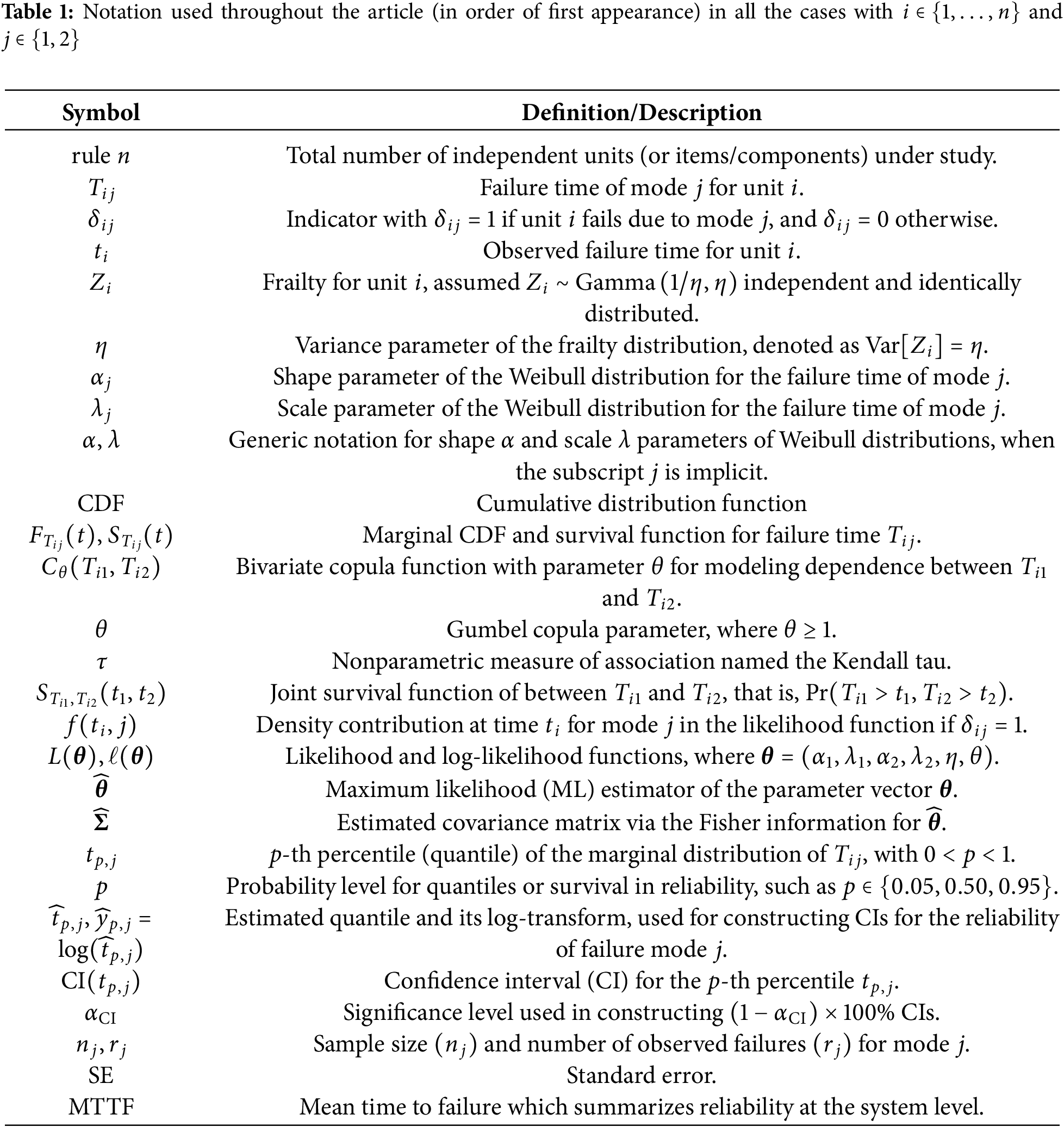
Throughout the article, we use a consistent set of symbols and acronyms, which are listed in Table 1 in the order of first appearance. Sections are arranged as follows. Section 2 provides background of copula-based methods and frailty models for reliability analysis. In Section 3, we describe the methodology for modeling competing risks data. In Section 4, CIs are constructed for dependent systems under ML estimation and delta-method. Section 5 conducts simulations, showing the roles of dependence and censoring in coverage probabilities (CPs) for Weibull-distributed failure times. In Section 6, we offer a synthetic example illustrating how penalized estimation can handle degenerate Hessian matrices under strong dependence and small samples. Section 7 concludes with findings and ideas for future research.
In this section, we present two main approaches in reliability analysis: copula-based methods for capturing dependence and frailty models for handling unobserved heterogeneity. These approaches form the basis for our proposed competing risks model with dependent failure times.
2.1 Copula-Based Methods for Dependency Structures
Copula-based methods are especially helpful for modeling the system reliability when component failures are dependent. These methods allow analysts to separate the marginal failure-time behavior from the joint dependence structure. Such methods are essential in real-world applications, where the assumption of independence among components is often unrealistic.
In essence, a copula is a bivariate cumulative distribution function (CDF) defined on the unit square
Definition 1: A bivariate copula is a function
(i) Boundary conditions–For all
(ii) Two-increasing property–For all
Definition 1 ensures that the copula encodes the dependence between two random variables.
Because a copula has uniform marginals on
Theorem 1 (Sklar): Let
The Sklar result presented in Theorem 1 underpins much of copula theory by separating marginal distributions from the dependence structure. This remains true in bivariate and multivariate contexts [18].
Corollary 1: Let F be a joint CDF of
An immediate implication of the Sklar theorem is that the product copula
2.2 Frailty Models for Failure Times in Competing Risks
Traditional reliability analysis often assumes that failure times are mutually independent. However, this assumption is frequently violated in systems where dependence exists. Correlated frailty models, as discussed in [33], offer a convenient framework for incorporating such dependence.
Parametric and semiparametric Bayesian frailty models [34] also handle shared risks effectively. Moreover, various estimation and extension approaches (such as the expectation-maximization algorithm for semiparametric hazards [35], and the developments presented in [36,37]) further enhance the modeling of correlated failure times under frailty frameworks.
A typical frailty model consists of three main parts as follows [38]:
• A frailty term representing latent or unobserved heterogeneity.
• A baseline risk function, which can be either parametric or nonparametric.
• An optional fixed-effects term to incorporate observed covariates.
Based on [24], we adopt a gamma distributed frailty to account for unobserved heterogeneity when modeling the failure times of two components using the Weibull distribution under competing risks. This adoption captures additional dependence arising from latent factors that affect both modes of failure in a single unit. In addition, we adapt the CI construction proposed in [39] to incorporate both the covariance structure of our frailty model and the dependence parameter of the copula. This provides a robust framework for inference on the system reliability when failure times are dependent.
In many real scenarios involving multiple competing risks, accurately capturing the interplay between shared risks (through a frailty) and direct dependence (through a copula) is critical. Therefore, we propose a framework merging both frailty and copula components to achieve a comprehensive characterization of the system reliability with dependent competing failure modes.
2.3 Advantages of the Proposed Framework
By combining a gamma-distributed frailty with a specific copula (here, the Gumbel family), our frailty-copula approach offers the following advantages:
• It captures unobserved heterogeneity through the latent variable
• It enables conditional tail dependence beyond what a simple frailty model can account for—an effect introduced through the Gumbel copula structure. This is especially valuable in high-risk scenarios where correlated early failures can occur more often than basic models suggest.
These two sources of dependence –the gamma distributed frailty
3 Modeling Competing Risks with Dependent Failure Times
In this section, we first present and adapt the frailty-copula framework introduced in [24], focusing on a two-component system with Weibull distributed failure times under competing risks. Then, we go beyond [24] by deriving CIs for marginal quantiles via a log-transformed delta method, fully incorporating both the frailty parameter
3.1 Competing Risks Model with Gamma Distributed Frailty and Gumbel Copula
In reliability terms, two failure time variables,
We adopt the Weibull distribution for each failure time, due to its well-established versatility in reliability contexts. It is capable of modeling various hazard shapes, such as increasing, constant, or decreasing failure rates. Nevertheless, our frailty-copula construction is not intrinsically limited to the Weibull model. In principle, other parametric forms—such as a generalized linear exponential distribution—could be used if prior knowledge or data analyses suggest a hazard structure not adequately captured by the Weibull model. In practice, implementing such alternatives often requires re-deriving the likelihood contributions for the copula-frailty model, which may lead to integrals without closed-form solutions and additional numerical complexity.
Moreover, with small sample sizes or strong dependence, identifiability of the extra parameters can pose further challenges. Given the broad applicability and familiarity of the Weibull model in engineering, we focus on that baseline here, noting that extensions to other parametric families remain viable future avenues under the same modeling framework. Hence, within this formulation based on the Weibull distribution, each failure time
The proposed model accounts for two distinct sources of dependence: (i) unobserved heterogeneity, captured by a gamma distributed frailty
In this study, we mainly adopt the viewpoint of two failure modes competing for the same item, but our formulas also apply to a two-component series arrangement with minimal modifications.
The Weibull distributed baseline and other options are considered next. Following [24] and usual practice in reliability studies, we adopt a Weibull distribution for each failure time. This adoption is motivated by the flexibility of the Weibull model in describing a range of hazard shapes and its common usage in engineering contexts. Although we focus on the Weibull distribution here, the framework can accommodate other parametric baselines (for example, exponential, gamma, generalized linear hazard distributions), or even semiparametric models, if domain knowledge or data characteristics suggest a different modeling strategy. In particular, a generalized linear exponential distribution could also be utilized within the same frailty-copula structure, albeit with different hazard formulations and potentially more challenging estimation details.
Next, we describe the gamma-distributed frailty. We introduce a gamma distributed frailty variable
Given
To induce dependence between
Hence, the joint conditional survival function of
Remark [Model identifiability]: Including both the gamma-frailty variance
Some implications and special cases are the following. Our frailty-copula method captures two complementary types of dependence: (i) extra-multiplier risk factors via
Even though this independence assumption given
3.2 Marginal Survival and Quantiles
Regardless of the specific copula, the marginal survival function for mode
Hence, the marginal
Thus, although the joint distribution may be complex, the marginal survival functions and quantiles emerge in closed form. This feature proves convenient for constructing reliability-based CIs and for evaluating system-level performance measures.
3.3 Mean and Variance of Marginal Failure Times
In the simpler gamma-Weibull mixture model setting, where each unit experiences a single failure mode and no additional copula structure is introduced, closed-form expressions for the mean and variance of the marginal failure times can be obtained.
Consider the shape and scale parameters
Then, the variance follows immediately, for
Note that, as
3.4 Dependence Structure and Identifiability in Competing Risks
Introducing a Gumbel copula
where
generally lacks a closed-form expression. Consequently, joint reliability metrics must be evaluated via numerical quadrature or other approximation methods. This copula-frailty structure is especially valuable for capturing potential tail dependence that goes beyond what is explained by shared frailty alone.
A natural way to measure and interpret the strength of such dependence in reliability studies is through the Kendall tau, denoted by
However, an important practical challenge arises because only the earliest failure time and its cause are typically observed in competing risks. This partial information can make it difficult to disentangle the roles of shared frailty (governed by
4 Maximum Likelihood Inference
In this section, we estimate the model parameters using the ML method and construct CIs for the reliability of dependent systems based on the ML estimation and delta methods.
We outline parameter estimation via the ML method. Consider
The likelihood function for observed data
where
Under the frailty-copula model, the joint survival function
Since
In practice, several considerations are essential to achieve robust inference. First, to avoid numerical instability or overflow, one can optimize
4.2 Confidence Intervals for Marginal Quantiles
We now focus on constructing CIs for the marginal quantiles
Specifically, if
In terms of practical implementation, evaluating
4.3 Asymptotic Validity and Coverage
Under usual regularity conditions, ensuring that
By applying a log-transformation and the delta method, we obtain a theoretically justified procedure for constructing CIs for
Specifically, let
as
(i) Consistency and asymptotic normality of the ML estimator distribution
(ii) Smoothness of the mapping from
(iii) Sufficient effective sample size for each mode
When conditions (i), (ii), and (iii) above are met, traditional asymptotic theory [33,38] implies that
as
Thus, exponentiating the bounds restores a suitable CP level on the original time scale. In practice, one can further corroborate these asymptotic results via simulation studies or bootstrap resampling to assess finite-sample performance.
4.4 Implicit Differentiation and Partial Derivatives
Because
where
where
Under usual regularity assumptions, including the consistency and asymptotic normality of
4.5 Taylor Expansions and Coverage Probability
To further elucidate why the proposed CIs converge to the nominal level, we use a Taylor expansion of the estimated marginal survival function
By expanding
where
An analogous argument applies to the lower bound
4.6 Asymptotic Normality and Slutsky Theorem
Under regularity conditions ensuring that
In summary, the asymptotic validity of our interval estimators for
This section describes a simulation study aimed at evaluating our proposed CIs for the reliability of a two-component series system, where component lifetimes follow Weibull distributions with a gamma-distributed frailty and are linked by a Gumbel copula. We assess the CPs of these CIs under different dependence levels (quantified by Kendall’s tau,
5.1 Setup and Frailty-Dependence Modeling
We adopt a gamma-distributed frailtyZ to capture unobserved heterogeneity among units, governed by the variance parameter
5.2 Implementation and Comparison of Interval Methods
For each generated dataset of size
• We use integrate() (the base R adaptive quadrature routine) or simple Monte Carlo methods to evaluate the integrals over the gamma frailty distribution.
• We employ numDeriv for finite-difference approximations of partial derivatives, which are needed to compute
• We call optim() (BFGS or L-BFGS-B) for quasi-Newton optimization, facilitating parameter constraints (such as positivity of
Following the expression stated in (2), each observation
We adopt the procedure outlined in Algorithm 1 to obtain empirical CPs for the proposed CI methods. In each simulation replicate, we generate a latent gamma distributed frailty
After generating

Following the steps in Algorithm 1, we evaluate the CP for each triple
5.4 Dependence Levels and Scenarios without Censoring
We examine three levels of dependence for Weibull-distributed failure times: weak, moderate, and strong. These are measured via the conditional Kendall’s tau, denoted by
5.5 Simulations with Complete Data (No Censoring)
To first isolate the effect of dependence on coverage, we consider the no-censoring case (0%). Tables 2–4 show the estimated 95% CPs for various sample sizes and quantiles
•
•
•

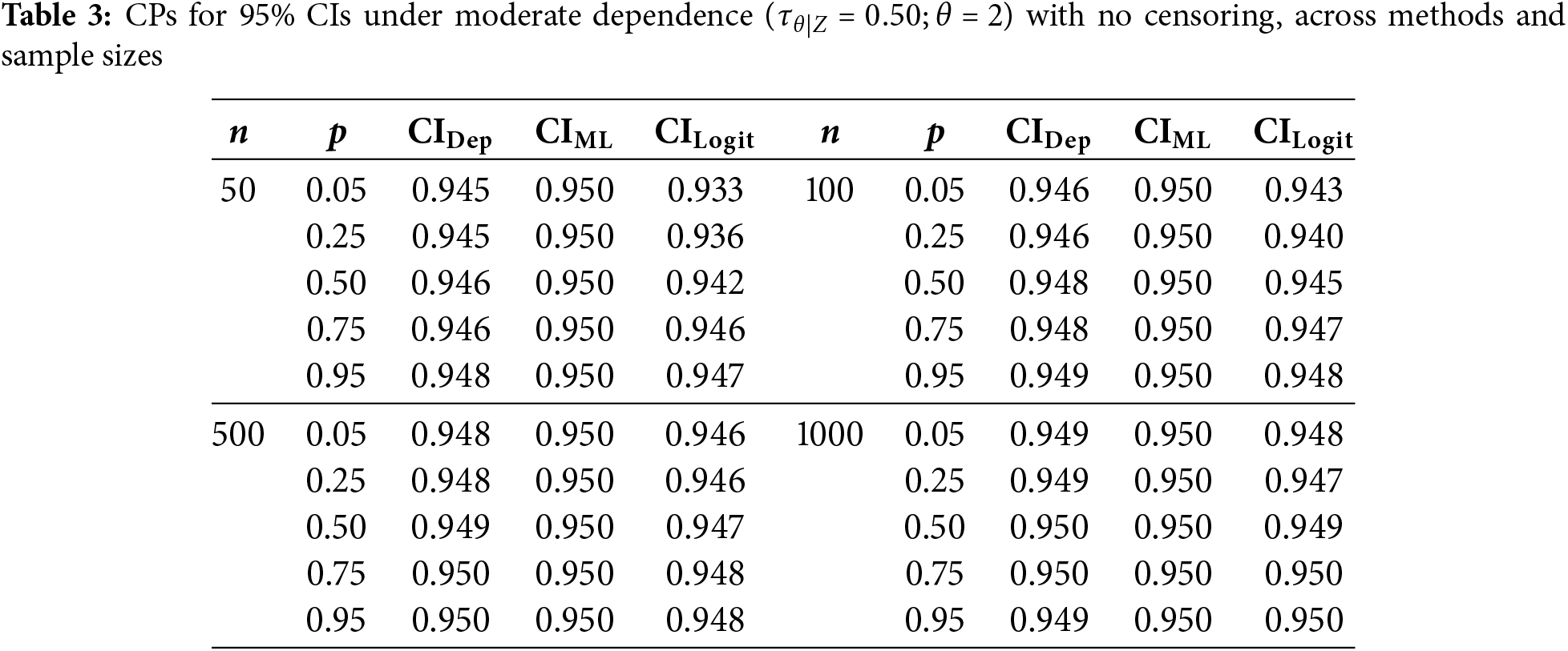
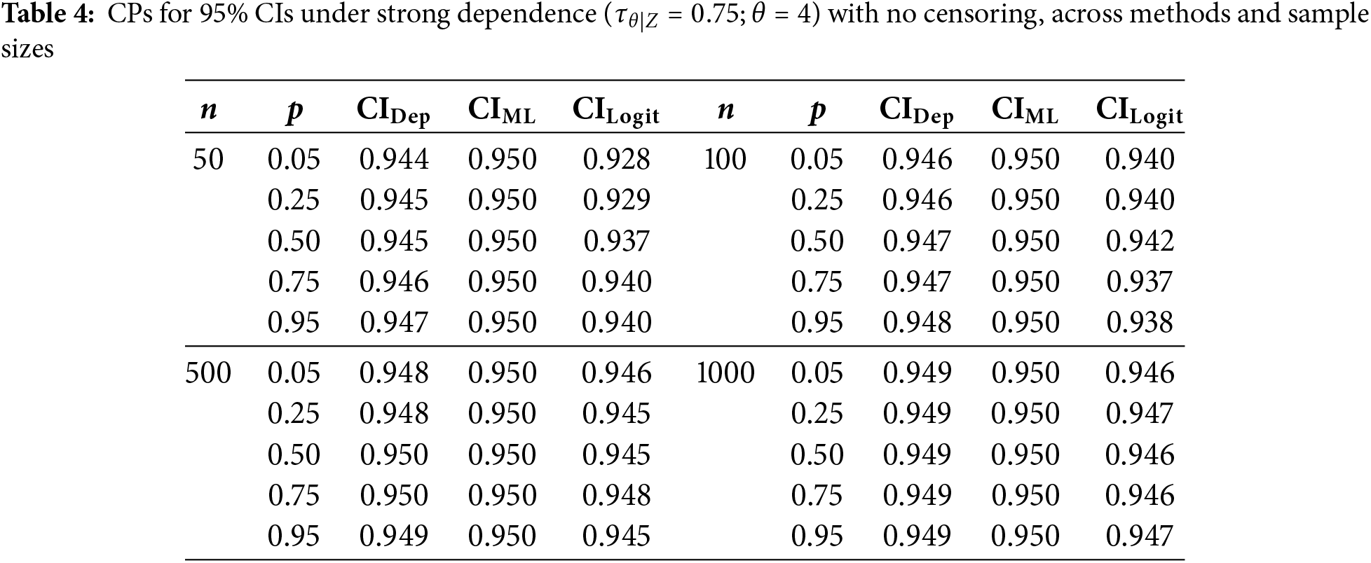
Fig. 1 summarizes the simulation design. Subsequent sections present analogous CP results under 10% and 25% censoring to represent more realistic scenarios with partially observed lifetimes.
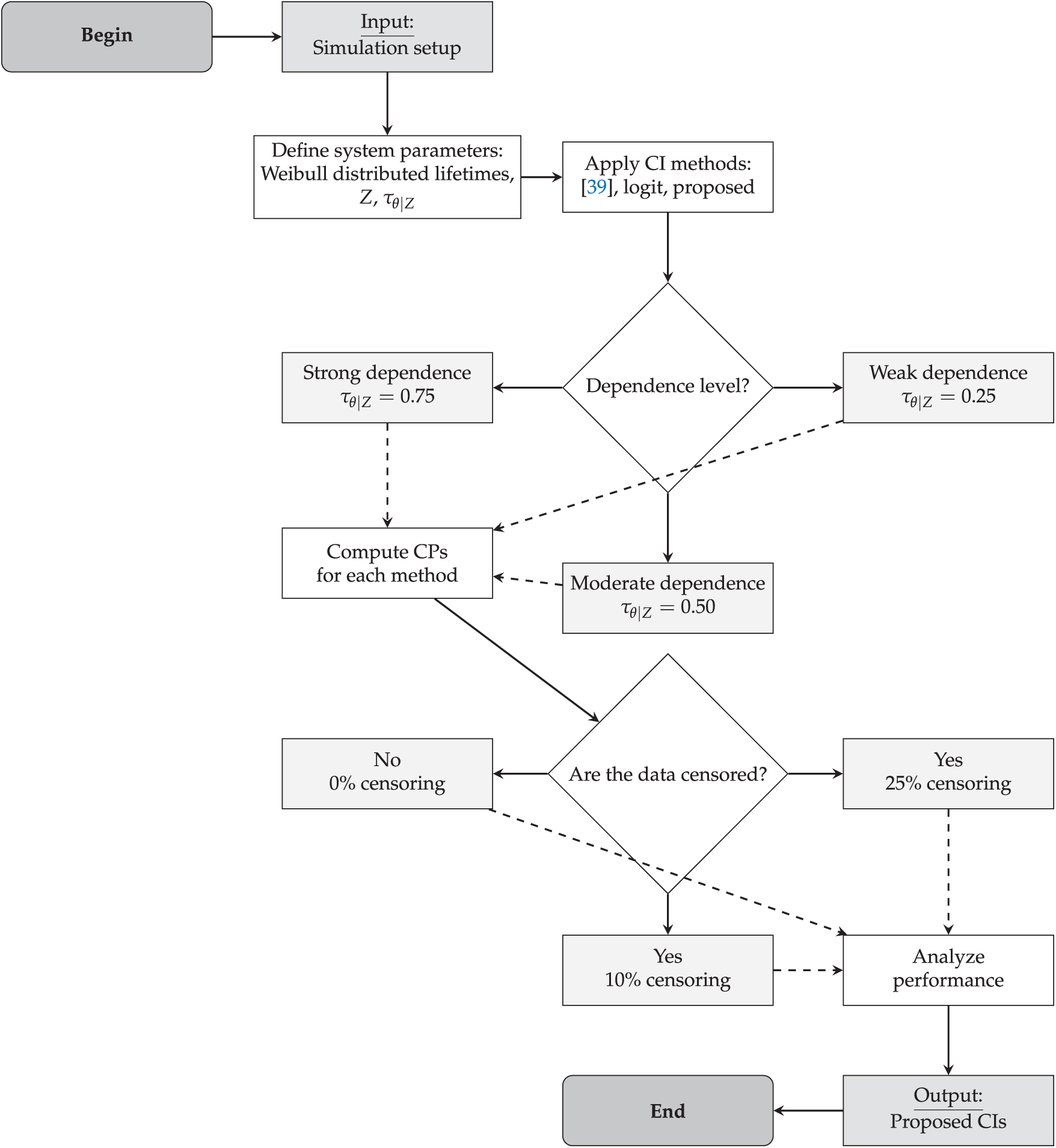
Figure 1: Flowchart of the simulation process for evaluating the impact of frailty on system reliability [39]
For the case of weak dependence,
In the case of moderate dependence,
Under strong dependence,
Overall, sample size still plays a role in CP performance, with all methods converging toward the nominal 95% as
5.6 Effect of Censoring on Confidence Interval Coverage
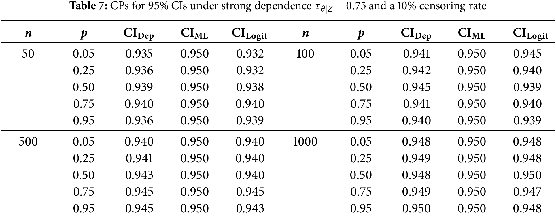
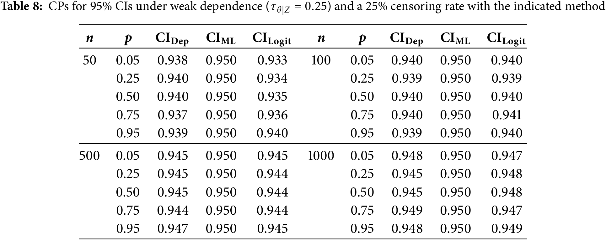
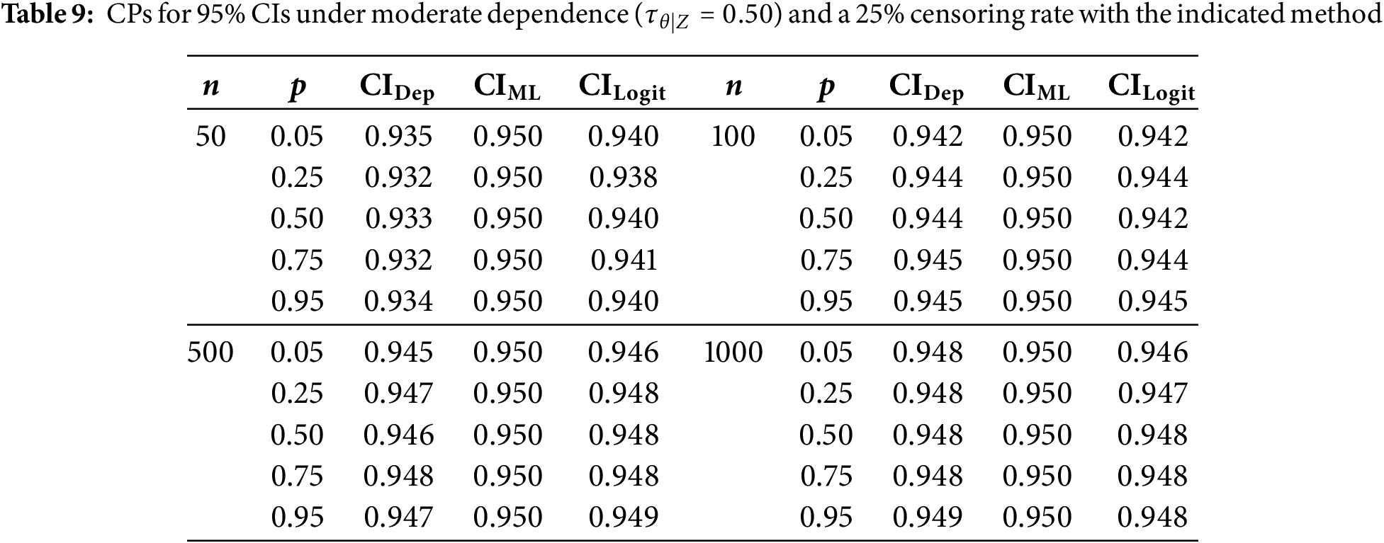
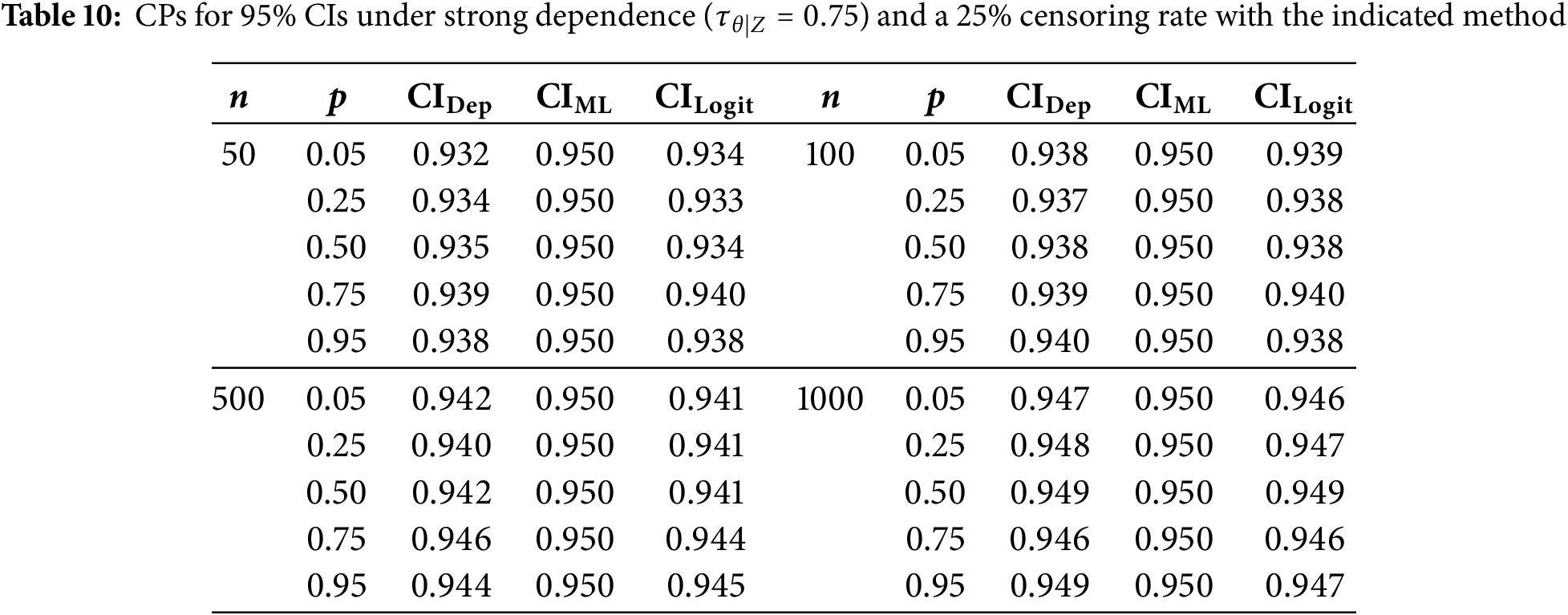
We now evaluate how additional right-censoring affects CPs under the same configurations stated in Section 5.4. Specifically, we apply 10% and 25% censoring and report results in Tables 5–7 (for 10%) and Tables 8–10 (for 25%).
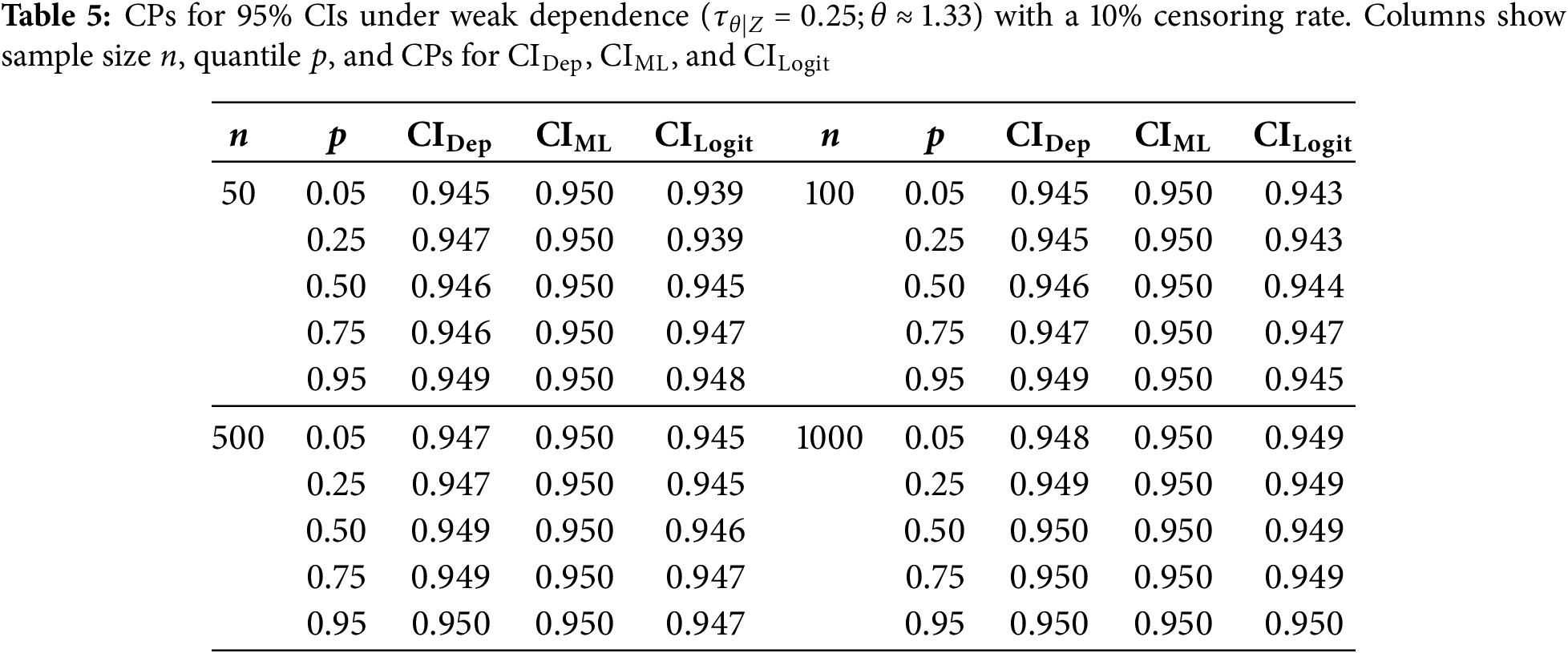
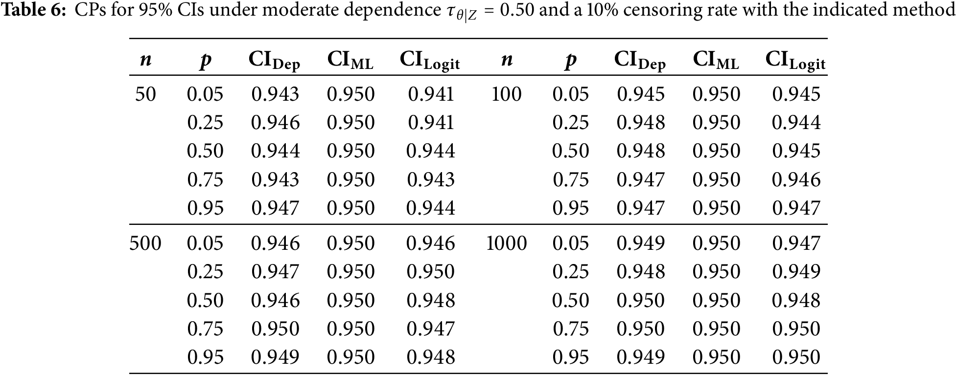
Under 10% censoring, CPs for smaller samples (
Moving to 25% censoring amplifies these differences somewhat, especially with strong dependence (
In summary, whether censoring is present or not, the adjusted CIs consistently provide CPs near the nominal level, especially in higher-dependence regimes and smaller sample sizes, where even slight improvements can be valuable. Hence, incorporating both the copula parameter
5.7 Impact of Dependence and Heterogeneity on System Reliability
Next, we investigate how varying the dependence among Weibull-distributed failure times affects both the system reliability and the mean time to failure (MTTF) in a two-component series system. Specifically, we adopt a Gumbel copula parameterized by
Table 11 summarizes our main results for reliability and MTTF, together with their bootstrap CIs. As expected for a series configuration, increasing dependence leads to lower reliability. Indeed, when
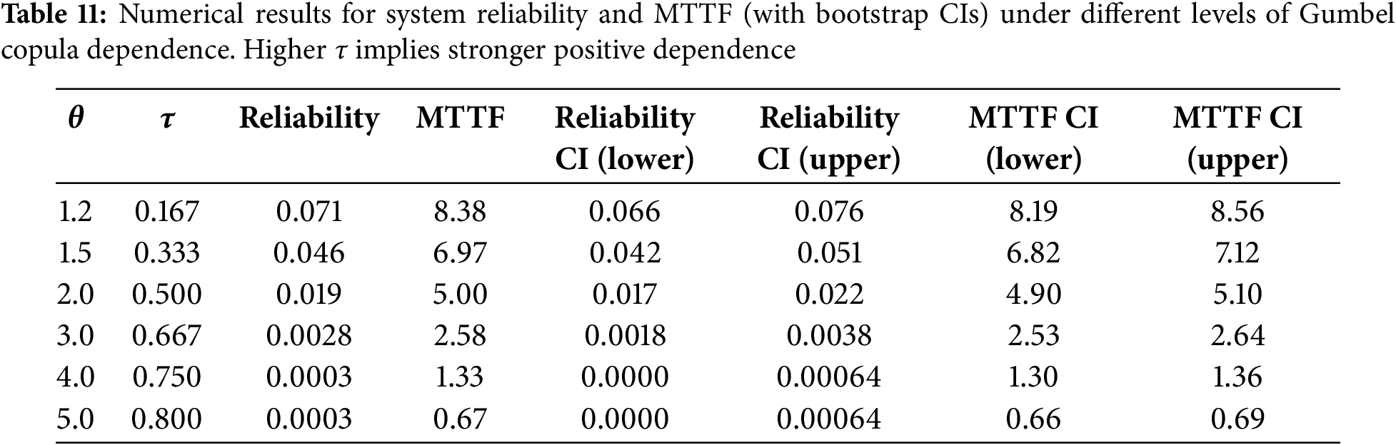
As
Overall, these findings highlight the importance of accurately modeling dependence in series systems. Greater positive dependence (higher
Future research may consider more complex or higher-dimensional dependence structures (such as multi-component series systems), as well as various censoring schemes, to further assess the stability of reliability estimation in strongly interdependent environments.
6 Illustrative Example with Penalized Estimation
In this section, we illustrate the practical implications of our method by conducting a synthetic case study designed to mimic a challenging real-world scenario. Specifically, we show how strong dependence, small samples, and estimation under a penalized likelihood framework can lead to non-trivial outcomes in practice. Here, we complement our previous discussion (see Section 5.7) on how dependence affects the system reliability and MTTF.
6.1 Rationale and Study Design
We consider a system of two-components connected in series for which each component time-to-failure follows a Weibull distribution (here taken as an exponential for simplicity), conditional on a gamma distributed frailty
6.2 Penalized Likelihood Function
As discussed in Section 4.1, ML estimation may suffer a degenerate Hessian matrix if the data exhibit strong dependence or the sample contains insufficient information to separate the copula and frailty parameters. To mitigate this degeneracy, we adopt a ridge-type penalization approach [39], adding a term
Fig. 2 sketches the simulation and estimation process. In one representative synthetic dataset, consider the following:
• We nominally set
• The data, however, had a far larger proportion of early failures than expected, with a definitive cause distribution of roughly
• Fitting via the ML estimate without penalization yielded a nearly singular Hessian matrix, preventing computation SEs and CIs.
• After imposing a moderate ridge penalty (
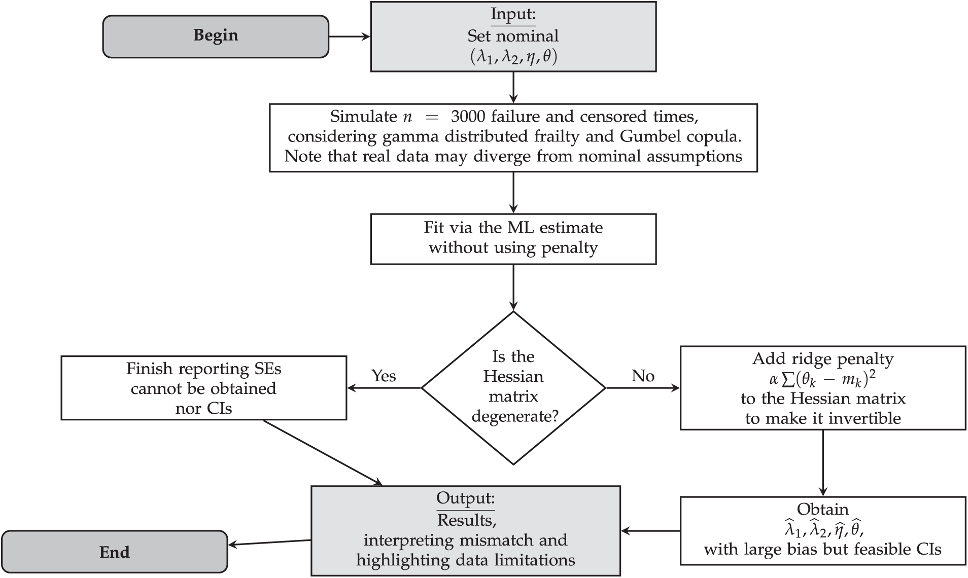
Figure 2: Flowchart illustrating penalized estimation in the challenging-data scenario. Without a penalty, the Hessian matrix may degenerate preventing SE computation. Adding a ridge penalty
6.4 Interpretation, Relevance, and Role of
Although the definitive estimates deviate sharply from
• Large values of
• Small values of
In a genuine industrial or engineering scenario, such results might appear if a system nominally expected to exhibit few failures (large
• Finite SEs to gauge how severely the data deviate from the nominal scenario.
• A strong signal that model assumptions may be misaligned (as evidenced by substantial parameter shifts and wide CIs).
Hence, from a reliability engineering viewpoint, even sophisticated models can become unstable if the data are insufficient or unrepresentative. Thus, incorporating penalization or prior knowledge helps to ensure a basic level of inferential robustness.
Although we do not present a real industrial dataset, this synthetic, real-like example is crafted to reflect high dependence and limited effective sample information. Practitioners commonly face similarly uncooperative data (sparse, heavily censored, or dominated by unanticipated early failures). Our penalized estimation strategy (frailty + copula + ridge) maintains a non-degenerate Hessian matrix, yielding SEs and CIs at the cost of potential bias. In realistic contexts, engineers may combine these estimates with domain expertise, covariate adjustments, or additional reliability testing to ease identifiability concerns. Overall, this synthetic, real-like study underlines the importance of robust or penalized approaches under strong dependence and sparse data. They avert numerical degeneracies and elucidate the degree of uncertainty, even if the ultimate parameter estimates deviate profoundly from nominal values.
In this article, we developed confidence intervals for dependent failure times in a two-component system, using Weibull distributed failure times combined with gamma distributed frailty and copula-based dependence. By explicitly including the copula parameter in the variance-covariance structure, our adjusted confidence intervals provide robust coverage probability under small samples and strong dependence—conditions where traditional methods can deviate from the nominal level.
Numerical experiments revealed that, while the traditional confidence intervals often remain close to their nominal coverage probability under moderate dependence or larger samples, they may underestimate variability in more challenging scenarios. In contrast, we found the proposed confidence intervals consistently maintain near-nominal coverage probability, even with up to 25% censoring. These findings underscore the practical gains from fully modeling both observed and unobserved heterogeneity, especially in high-dependence or data-sparse applications.
We further illustrated our analysis in a penalized estimation study with a synthetic real-like example, where we simulated data under nominal parameters
Although our study focused on two-component systems connected in series, extending this study to higher-dimensional settings is feasible but will face additional identifiability and computational complexities. Likewise, while we employed the Weibull distribution for its flexibility and frequent use in reliability contexts, alternative baselines (such as the exponential, gamma, or Birnbaum-Saunders distributions [43]) could be explored if data or expert knowledge suggests different hazard shapes. Moreover, although we illustrated the Gumbel and Clayton copulas for positive dependence, our framework accommodates other families, especially those capturing distinct tail behaviors, to match real-world failure patterns more closely.
Despite the strengths identified in our study, certain limitations remain. Greater systems may require stronger identifiability constraints or Bayesian/regularization strategies to separate frailty from copula effects reliably.
Further research could also examine semiparametric baselines and alternative censoring schemes [44,45]. Nonetheless, we believe that the proposed adjusted confidence intervals, by integrating both frailty and direct copula dependence, constitute a valuable tool for practical reliability analyses where correlated failures and small samples pose challenges, and that penalized variants of our estimation strategy offer a pragmatic fallback in highly demanding scenarios.
Acknowledgement: The authors thank the editors and anonymous reviewers for their insightful and constructive feedback. Their detailed comments and thoughtful suggestions improved the clarity, completeness, and theoretical foundation of this article. We sincerely appreciate the time and effort they dedicated to reviewing our work.
Funding Statement: The research of O. E. Bru-Cordero was supported by the Colombian government through COLCIENCIA scholarships, National Doctoral Program, Call 727 of 2015. C. Castro gratefully acknowledges partial financial support from the Centro de Matemática da Universidade do Minho (CMAT/UM), through UID/00013. V. Leiva acknowledges funding from the Agencia Nacional de Investigación y Desarrollo (ANID) of the Chilean Ministry of Science, Technology, Knowledge and Innovation, through FONDECYT project grant 1200525.
Author Contributions: All authors contributed to the conceptualization, methodology, and investigation of this research. Osnamir E. Bru-Cordero focused on the theoretical framework for frailty models and copula-based dependence structures, under the scientific supervision of Mario C. Jaramillo-Elorza and Víctor Leiva. Cecilia Castro led the overarching review and editing process, performed additional analyses, restructured the manuscript, and coordinated revisions in response to feedback. Víctor Leiva led the writing of the initial draft and subsequent revisions until the final submission. Mario C. Jaramillo-Elorza and Víctor Leiva supervised the overall study design, including the simulation scenarios and the critical review of the manuscript. All authors reviewed the results and approved the final version of the manuscript.
Availability of Data and Materials: The codes and data are available under request from the authors.
Ethics Approval: Not applicable. The research does not involve human or animal subjects.
Conflicts of Interest: The authors declare no conflicts of interest to report regarding the present study.
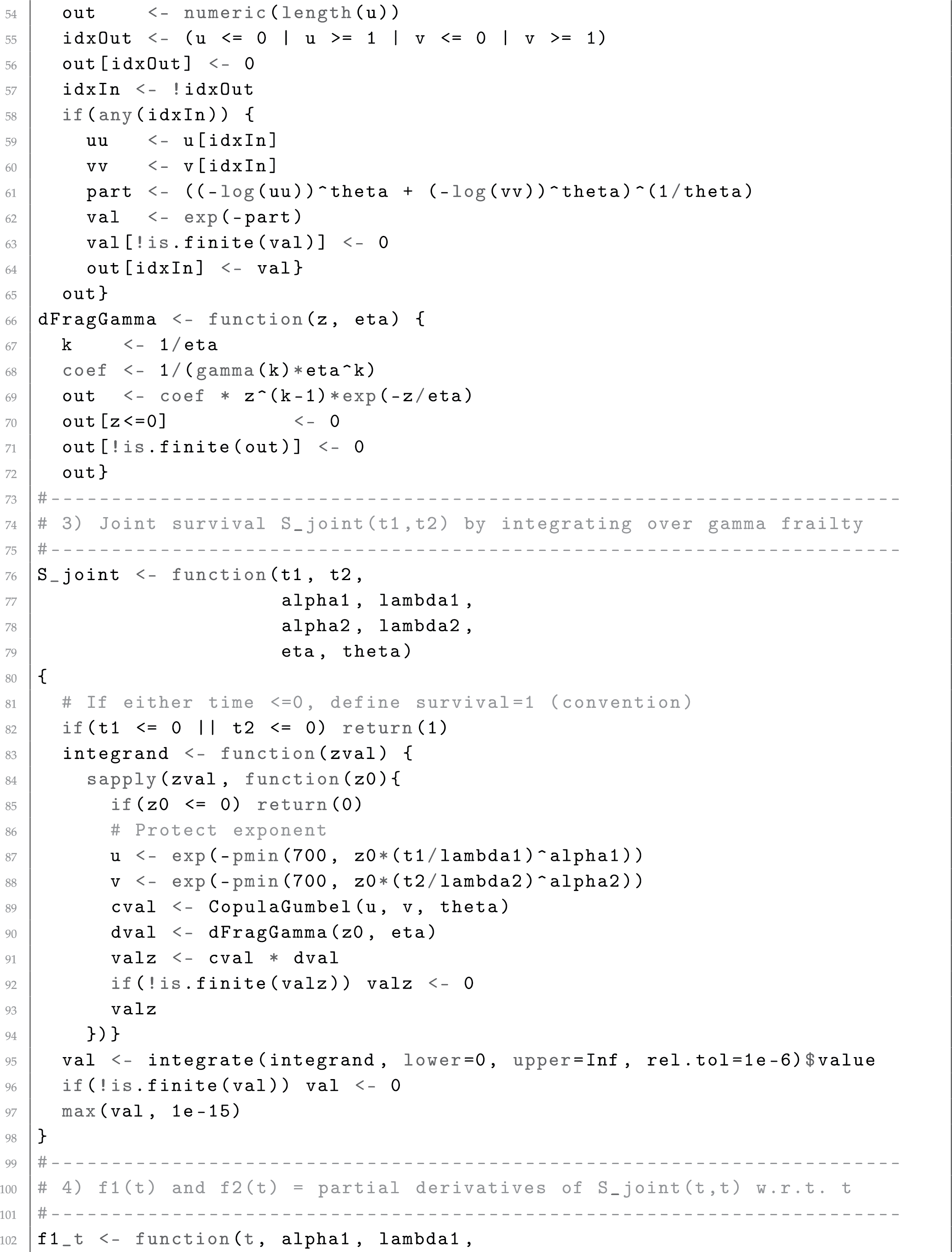
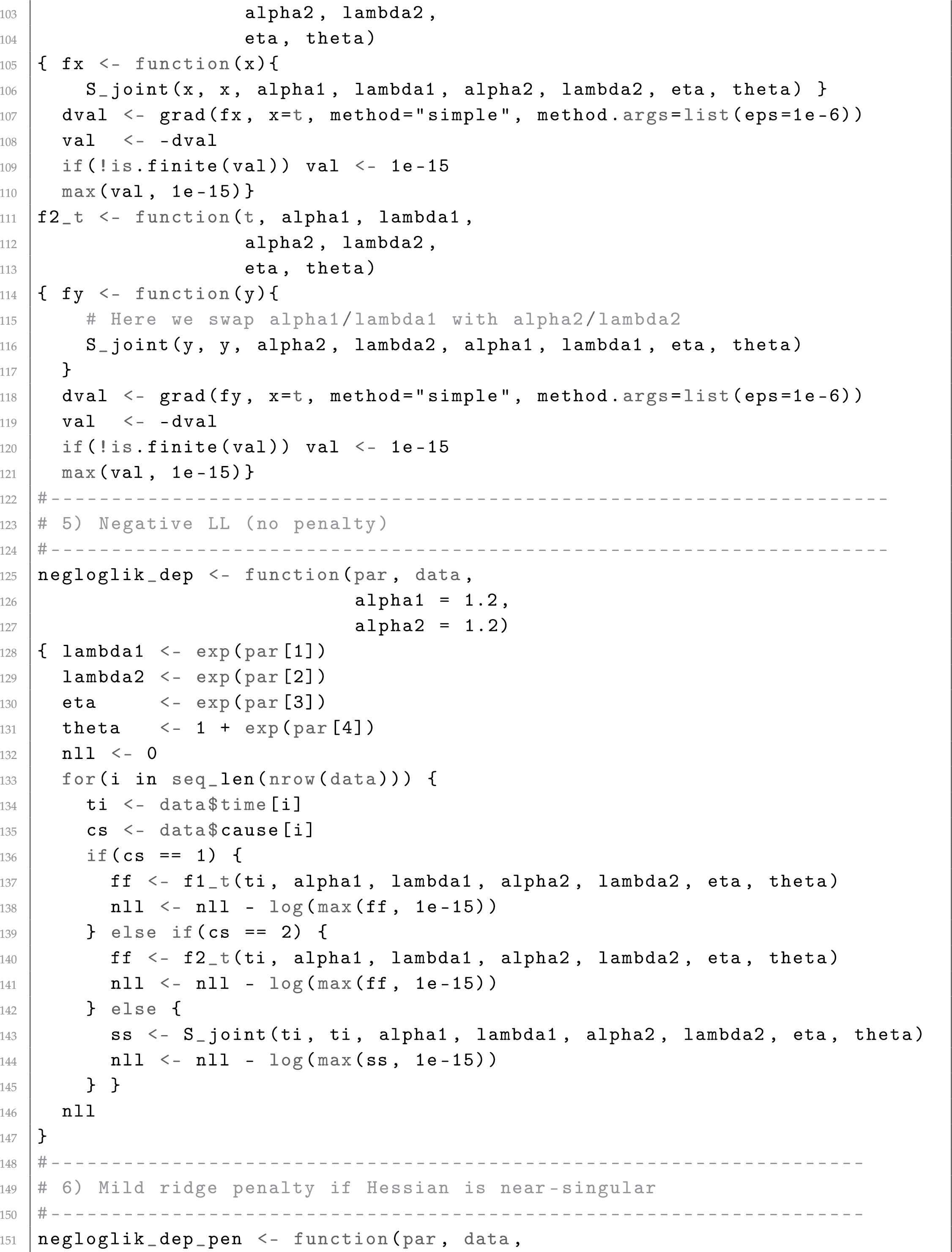
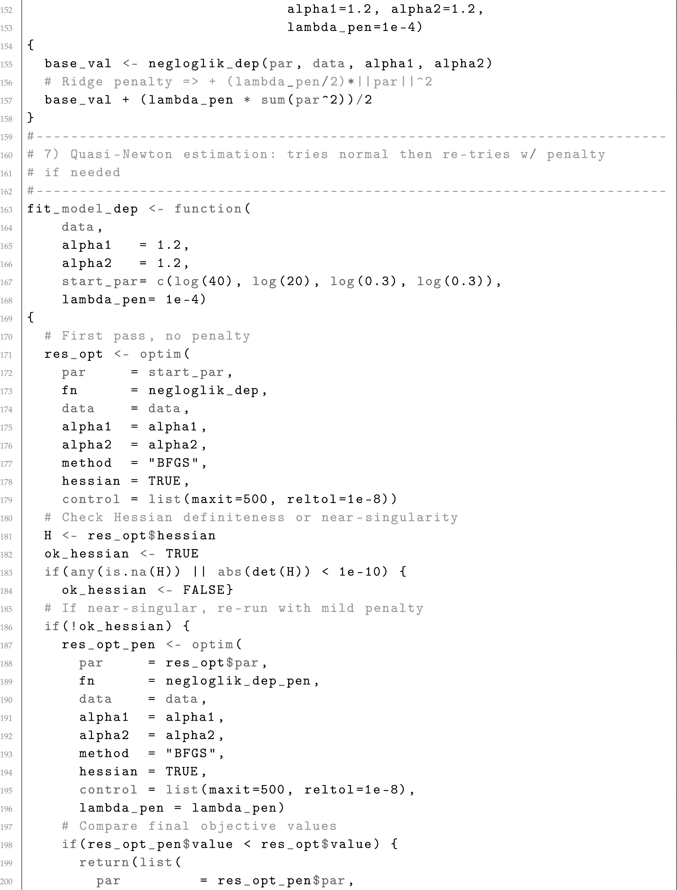
Appendix A R Script for Penalized Estimation and
This appendix provides an illustrative R script implementing data generation via a gamma-frailty Gumbel-copula model, quasi-Newton parameter estimation with a mild ridge penalty when the Hessian is nearly singular, and the construction of


References
1. Li H, Peng W, Adumene S, Yazdi M. Cutting edge research topics on system safety, reliability, maintainability, and resilience of energy-critical infrastructures. In: Intelligent reliability and maintainability of energy infrastructure assets. Cham, Switzerland: Springer; 2023. p. 25–38 doi:10.1007/978-3-031-29962-9_2. [Google Scholar] [CrossRef]
2. Osei-Kyei R, Almeida LM, Ampratwum G, Tam V. Systematic review of critical infrastructure resilience indicators. Constr Innov. 2023;23(5):1210–31. doi:10.1108/ci-03-2021-0047. [Google Scholar] [CrossRef]
3. Li Y, Bai X, Shi S, Wang S. Dynamic fatigue reliability analysis of transmission gear considering failure dependence. Comput Model Eng Sci. 2022;130(2):1077–92. doi:10.32604/cmes.2022.018181. [Google Scholar] [CrossRef]
4. Livingston D, Sivaram V, Freeman M, Fiege M. Applying blockchain technology to electric power systems. New York, NY, USA: Council on Foreign Relations; 2022. [Google Scholar]
5. Giraldo R, Leiva V, Christakos G. Leverage and Cook distance in regression with geostatistical data: methodology, simulation, and applications related to geographical information. Int J Geogr Inf Sci. 2023;37(3):607–33. doi:10.1080/13658816.2022.2131790. [Google Scholar] [CrossRef]
6. Aven T, Jensen U. Stochastic failure models. In: Stochastic models in reliability. New York, NY, USA: Springer; 2013. p. 57–103. [Google Scholar]
7. Wagner N. Comparing the complexity and efficiency of composable modeling techniques for multi-scale and multi-domain complex system modeling and simulation applications: a probabilistic analysis. Systems. 2024;12(3):96. doi:10.3390/systems12030096. [Google Scholar] [CrossRef]
8. Qiu J, Sun H, Wang S. Research progress of reverse Monte Carlo and its application in Josephson junction barrier layer. Comput Model Eng Sci. 2023;137(3):2077–109. doi:10.32604/cmes.2023.027353. [Google Scholar] [CrossRef]
9. Wang C. Structural reliability and time-dependent reliability. Cham, Switzerland: Springer; 2021. [Google Scholar]
10. Guiraud P, Leiva V, Fierro R. A non-central version of the Birnbaum-Saunders distribution for reliability analysis. IEEE Trans Reliab. 2009;58(1):152–60. doi:10.1109/tr.2008.2011869. [Google Scholar] [CrossRef]
11. Netes V, Sharov V. Common cause failures in communication networks. In: Proceedings of the 2024 Conference on Systems of Signals Generating and Processing in the Field of on Board Communications; 2024 Mar 12–14; Moscow, Russian Federation. p. 1–7. [Google Scholar]
12. Meeker WQ, Escobar LA, Pascual FG. Statistical methods for reliability data. New York, NY, USA: Wiley; 2022. [Google Scholar]
13. Octavina S, Lin SW, Yeh RH. Copula-based Bayesian reliability assessment for series systems. Qual Reliab Eng Int. 2024;40(5):2444–55. doi:10.1002/qre.3514. [Google Scholar] [CrossRef]
14. Abuelamayem O. Reliability estimation of a multicomponent stress-strength model based on copula function under progressive first failure censoring. Stat Optim Inf Comput. 2024;12(6):1601–11. doi:10.19139/soic-2310-5070-1894. [Google Scholar] [CrossRef]
15. Zheng M, Klein JP. Estimates of marginal survival for dependent competing risks based on an assumed copula. Biometrika. 1995;82(1):127–38. doi:10.1093/biomet/82.1.127. [Google Scholar] [CrossRef]
16. Barlow R, Proschan F. Statistical theory of reliability and life testing: probability models. New York, NY, USA: Wiley; 1975. [Google Scholar]
17. Navarro J, Durante F. Copula-based representations for the reliability of the residual lifetimes of coherent systems with dependent components. J Multivar Anal. 2017;158:87–102. doi:10.1016/j.jmva.2017.04.003. [Google Scholar] [CrossRef]
18. Nelsen RB. An introduction to copulas. New York, NY, USA: Springer; 2006. [Google Scholar]
19. Leiva V, dos Santos RA, Saulo H, Marchant C, Lio Y. Bootstrap control charts for quantiles based on log-symmetric distributions with applications to the monitoring of reliability data. Qual Reliab Eng Int. 2023;39(1):1–24. doi:10.1002/qre.3072. [Google Scholar] [CrossRef]
20. Aalen O, Borgan O, Gjessing H. Survival and event history analysis: a process point of view. New York, NY, USA: Springer; 2008. [Google Scholar]
21. Mokkink LB, de Vet H, Diemeer S, Eekhout I. Sample size recommendations for studies on reliability and measurement error: an online application based on simulation studies. Health Serv Outcomes Res Methodol. 2023;23(3):241–65. doi:10.1007/s10742-022-00293-9. [Google Scholar] [CrossRef]
22. Brown B, Liu B, McIntyre S, Revie M. Reliability evaluation of repairable systems considering component heterogeneity using frailty model. Proc Inst Mech Eng O J Risk Reliab. 2023;237(4):654–70. doi:10.1177/1748006x221109341. [Google Scholar] [CrossRef]
23. Gorfine M, Zucker DM. Shared frailty methods for complex survival data: a review of recent advances. Annu Rev Stat Appl. 2023;10(1):51–73. doi:10.1146/annurev-statistics-032921-021310. [Google Scholar] [CrossRef]
24. Wang YC, Emura T, Fan TH, Lo SM, Wilke RA. Likelihood-based inference for a frailty-copula model based on competing risks failure time data. Qual Reliab Eng Int. 2020;36(5):1622–38. doi:10.1002/qre.2650. [Google Scholar] [CrossRef]
25. Leao J, Leiva V, Saulo H, Tomazella V. Incorporation of frailties into a cure rate regression model and its diagnostics and application to melanoma data. Stat Med. 2018;37(29):4421–40. doi:10.1002/sim.7929. [Google Scholar] [PubMed] [CrossRef]
26. Calsavara VF, Tomazella V, Fogo JC. The effect of frailty term in the standard mixture model. Chil J Stat. 2013;4(2):95–109. [Google Scholar]
27. Wang YC, Emura T. Multivariate failure time distributions derived from shared frailty and copulas. Jpn J Stat Data Sci. 2021;4(2):1105–31. doi:10.1007/s42081-021-00123-1. [Google Scholar] [CrossRef]
28. Rouzbahani M, Akhoond MR, Chinipardaz R. A new bivariate survival model with a cured fraction: a mixed Poisson frailty-copula approach. Jpn J Stat Data Sci. 2025;11(4):261. doi:10.1007/s42081-023-00240-z. [Google Scholar] [CrossRef]
29. Liu X. Planning of accelerated life tests with dependent failure modes based on a gamma frailty model. Technometrics. 2012;54(4):398–409. doi:10.1080/00401706.2012.707579. [Google Scholar] [CrossRef]
30. Lu JC, Bhattacharyya GK. Some new constructions of bivariate Weibull models. Ann Inst Stat Math. 1990;42(3):543–59. doi:10.1007/bf00049307. [Google Scholar] [CrossRef]
31. Murthy DP, Xie M, Jiang R. Weibull models. New York, NY, USA: Wiley; 2004. [Google Scholar]
32. Escarela G, Carriere J. Fitting competing risks with an assumed copula. Stat Methods Med Res. 2003;12(4):333–49. doi:10.1191/0962280203sm335ra. [Google Scholar] [PubMed] [CrossRef]
33. Duchateau L, Janssen P. The frailty model. New York, NY, USA: Springer; 2007. [Google Scholar]
34. Ibrahim JG, Chen MH, Sinha D. Bayesian survival analysis. Hoboken, NJ, USA: Wiley; 2014. [Google Scholar]
35. Tableman M, Kim JS. Survival analysis using S: analysis of time-to-event data. Boca Raton (FLCRC Press; 2003. [Google Scholar]
36. Hougaard P. Analysis of multivariate survival data. New York, NY, USA: Springer; 2012. [Google Scholar]
37. Lin H, Zelterman D. Modeling survival data: extending the cox model. New York, NY, USA: Taylor and Francis; 2002. [Google Scholar]
38. Wienke A. Frailty models in survival analysis. Boca Raton, FL, USA: Chapman & Hall/CRC; 2010. [Google Scholar]
39. Hong Y, Meeker WQ. Confidence intervals for system reliability and applications to competing risks models. Lifetime Data Anal. 2014;20(2):161–84. doi:10.1007/s10985-013-9245-9. [Google Scholar] [PubMed] [CrossRef]
40. Vallejos CA, Steel MF. Incorporating unobserved heterogeneity in Weibull survival models: a Bayesian approach. Econom Stat. 2017;3(2):73–88. doi:10.1016/j.ecosta.2017.01.005. [Google Scholar] [CrossRef]
41. Emura T, Nakatochi M, Murotani K, Rondeau V. A joint frailty-copula model between tumour progression and death for meta-analysis. Stat Methods Med Res. 2017;26(6):2649–66. doi:10.1177/0962280215604510. [Google Scholar] [PubMed] [CrossRef]
42. Tsiatis A. A nonidentifiability aspect of the problem of competing risks. Proc Natl Acad Sci USA. 1975;72(1):20–2. doi:10.1073/pnas.72.1.20. [Google Scholar] [PubMed] [CrossRef]
43. Leiva V, Castro C, Vila R, Saulo H. Unveiling patterns and trends in research on cumulative damage models for statistical and reliability analyses: bibliometric and thematic explorations with data analytics. Chil J Stat. 2024;15:81–109. [Google Scholar]
44. Barros M, Leiva V, Ospina R, Tsuyuguchi A. Goodness-of-fit tests for the Birnbaum-Saunders distribution with censored reliability data. IEEE Trans Reliab. 2014;63(2):543–54. doi:10.1109/tr.2014.2313707. [Google Scholar] [CrossRef]
45. Cárcamo E, Marchant C, Ibacache-Pulgar G, Leiva V. Birnbaum-Saunders semi-parametric additive modeling: estimation, smoothing, diagnostics and application. REVSTAT Stat J. 2024;22:211–37. doi:10.57805/revstat.v22i2.483. [Google Scholar] [CrossRef]
Cite This Article
 Copyright © 2025 The Author(s). Published by Tech Science Press.
This work is licensed under a Creative Commons Attribution 4.0 International License , which permits unrestricted use, distribution, and reproduction in any medium, provided the original work is properly cited.
 Downloads
 Citation Tools