Feasibility of Using Optimal Control Theory and Training-Performance Model to Design Optimal Training Programs for Athletes

1  Introduction

The main goal of athletic training planning is to help athletes achieve the best performances in competitions [1]. One of the most important responsibilities of coaches and trainers is to design optimal training programs to help athletes reach this goal. Though this goal is clear and straightforward, its execution in practice is often far from optimal. Traditionally, coaches and trainers primarily rely on their subjective opinions, experiences, as well as trials and errors, but rely relatively little on scientific evidence and analyses for designing training programs [2,3]. It is conceivable that this traditional philosophy of designing training programs could not guarantee to help athletes reach their most important goal, i.e., having optimal physical fitness and achieving the best performance on the competition day. In order to help athletes optimize their performances in competitions while prevent overtraining and the risk of overuse injuries, it is important to develop science-based strategies for optimally designing training programs.

The relationship between training and athletic performance is multi-factorial, and therefore is a complex problem [4]. For the sake of better understanding the relationship between training and performance with the goal of helping athletes optimize their performances, scientists have developed mathematical models of training and performance (termed “training-performance models” in the following content) [1,3–6]. Training-performance models provide a science-based, quantitative method for understanding the effects of training on performance and the relationship between training and performance, as well as predicting an athlete’s performance over time during the training course and on the competition day. Since the introduction of the Banister impulse-response (IR) model (the earliest proposed training-performance model) [7,8], a number of training-performance models modified from the Banister IR model have been subsequently proposed [9–13]. One of the main advantages of training-performance models is that they can be applied to design training programs for an individual, since the model input is the data collected from an individual and therefore the model output is specific to that individual [3]. Given a hypothetical training program (i.e., daily training loads during the training course) and the model parameters determined from an individual as the inputs of the model, a training-performance model could quantitatively describe and predict an athlete’s performance over time during the training course and on the competition day based on this hypothetical training program, and thereby evaluate the optimality and efficacy of this hypothetical training program for this individual.

Traditionally, in the applications of using training-performance models to design optimal training programs, researchers resort to successive simulations based on a trial-and-error procedure [3,4]. Successive simulations are conducted by designing many different hypothetical training programs and inputting them into the model one by one. For each hypothetical training program, the performance on the competition day is predicted by solving the model. Then, among the designed hypothetical training programs, the one that generates the highest performance can be found. However, it can be understood that the theoretical optimal training program that generates the best performance for an individual could not be easily found by using this trial-and-error simulation procedure. Nowadays, data science and data-driven techniques have advanced rapidly, and these kinds of methods could allow more accurate and efficient assessment, and thereby more successful optimization of athletic performance. For example, Imbach et al. proposed that the combined use of machine learning techniques and training-performance models could improve and broaden the applications of training-performance models for athletic performance modeling [4]. Couceiro et al. proposed an ecological dynamics framework capable of merging a large amount of data into a smaller set of variables that results in a deeper and easier analysis, in order to allow sports scientists and practitioners to interpret data of athletes’ behaviors during training and competition in real-time for helping improve athletic performance [14]. Den Hartigh et al. proposed a multidisciplinary, dynamic and personalized approach applying knowledge and techniques of data science to improve the resilience of athletes [15].

Optimal control theory [16–20] is a powerful mathematical framework that aims to determine the optimal strategy to optimize a given objective functional for a dynamical system [21–23]. Optimal control theory has been applied in numerous fields, including agriculture [24–27], biology and medicine [28–31], economics and management [32–35] and engineering [36–39], to name a few. To the best of our knowledge, optimal control theory has not been applied to the fields of sports sciences and athletic training, and we believe that the combined use of optimal control theory and training-performance models could be a promising method for designing optimal training programs for helping athletes achieve the best performances in competitions more efficiently.

The purpose of the present study is to develop a novel method by the combined use of optimal control theory and a training-performance model for designing optimal training programs, in order to help athletes achieve the best performance exactly on the competition day while properly manage training load during the training course for preventing overtraining.

2  Materials and Methods

2.1 Background of the Training-Performance Model Used in the Proposed Optimal Control Framework

The purpose of this subsection is to introduce how the training-performance model used in the proposed optimal control framework is conceptually formulated. Since the training-performance model used in the proposed optimal control framework is a conceptual extension of the Banister IR model as will be explained below, the Banister IR model and some relevant background knowledge will be introduced in advance to lay the foundation for better understanding the essence of the training-performance model used in the proposed optimal control framework and how it is conceptually formulated.

In 1975, Banister and colleagues [7] posited that the response of athletic performance to training follows a first-order dynamical model of the form

p′(t)=−1τp(t)+kw(t),(1)

where t is time, p(t) and w(t) are performance and training load over time, respectively. τ and k are the time constant and gain term for p(t), respectively, and they are parameters relevant to the physiological characteristics of an athlete; these two parameters are positive real constants. Eq. (1) is the earliest and most fundamental training-performance model that has been served as a foundational framework for years in the fields of sports science and athletic training for quantitatively understanding the relationship between training and performance. It describes how performance decays over time naturally, and how training can either slow the decay of performance or improve performance; in other words, this model intends to describe the effects of training on performance. In the paper in which the Banister IR model was first proposed [7,8], this model was used to describe the relationship between training and performance of a competitive swimmer. Since then, the Banister IR model and the subsequent models modified based on it have been applied to numerous kinds of sports and have started to attract more interest in recent years owing to their important roles in commercially available portable devices for real-time exercise monitoring [3].

During the training course, performance can increase or decrease due to the effects of a number of factors (including regulation of training load). Hence, performance can be assumed to be the difference between the overall positive effects on performance (termed “fitness”) and the overall negative effects on performance (termed “fatigue”) plus the performance on the initial day [8], i.e., p(t)=p(0)+f(t)−u(t), where f(t) and u(t) are fitness and fatigue over time, respectively, and p(0) is the performance on the initial day.

If each of fitness and fatigue is assumed to follow the dynamical model of the form as Eq. (1), i.e., p′(t)=−1τp(t)+kw(t), a modified Banister IR model can be obtained as [13]

f′(t)=−1τ1f(t)+k1w(t),

u′(t)=−1τ2u(t)+k2w(t),

and

p(t)=p(0)+f(t)−u(t),(2)

where τ1, τ2 are two time constants and k1, k2 are two gain terms for f(t) and u(t), respectively, and they are parameters relevant to the physiological characteristics of an athlete; these four parameters are positive real constants. The first and second equations of Eq. (2) describe the dynamics of fitness and fatigue respectively, including the effects of training on these two variables. It can be observed that training load is the forcing term of the first-order differential equation governing the dynamics of fitness or fatigue, therefore, an increase in training load causes the change in fitness or fatigue to increase over time. Since fitness and fatigue represent positive and negative effects on performance, respectively, the equation for p(t) in Eq. (2) describes that performance is the sum of fitness minus fatigue plus the performance on the initial day. In the proposed optimal control framework, we use Eq. (2) as the training-performance model to describe the dynamics of performance, fitness, fatigue, and training load. The units of the variables and parameters in Eq. (2) in the proposed optimal control framework will be described below. Please see Section 1 of the supplementary material for a brief introduction regarding how fitness, fatigue, and training load are typically measured in experiments.

2.2 Formulation and Solution Methods of the Proposed Optimal Control Framework

In this subsection, we introduce the proposed optimal control framework and its solution methods. In the proposed optimal control framework, we use Eq. (2) as the training-performance model to describe the dynamics of performance, fitness, fatigue, and training load. The goal of the proposed optimal control framework is to maximize the fitness and minimize the fatigue on the competition day in order to maximize the performance on the competition day while minimize the cumulative training load during the training course. In the context of maintaining or even improving performance, minimize the cumulative training load during the training course can help an athlete prevent excessive training and fatigue that could lead to the reduction of performance and the increased risk of sports injuries. Hence, the proper management of the training load can help an athlete maintain the optimal physical and psychological conditions and minimize the likelihood of sports injuries. In addition, if an athlete can achieve the same (or even higher) performance with less training load, the athlete can have more time and energy for resting and activities other than training, therefore can have a better quality of life.

Hence, the objective functional of the proposed optimal control framework is

maxw[f(tp)−u(tp)−A∫0tpw2(t)dt],(3)

where tp is the number of days between the initial day of training and the competition day, and A is a parameter associated with the characteristics of an optimal training program, determining the value of the maximum daily training load and the number of days that an athlete trains with the maximum daily training load during the training course. These two parameters are prescribed constants in the simulation. The effects and practical implication of A will be further discussed in the Results and Discussion section.

Combining Eqs. (2) and (3), the proposed optimal control framework is formulated as

maxw[f(tp)−u(tp)−A∫0tpw2(t)dt](4)

subject to

f′(t)=−1τ1f(t)+k1w(t),f(0)=0,(5)

u′(t)=−1τ2u(t)+k2w(t),u(0)=0,(6)

M1≤w(t)≤M2,(7)

p(t)=p(0)+f(t)−u(t),p(0)=0,(8)

where w(t) is the control variable (which is a piecewise continuous function), while p(t), f(t) and u(t) are the state variables (which are continuous functions). M1 and M2 are the lower and upper bounds of w(t), respectively. Though the parameters and variables in the proposed optimal control framework can be in any suitable units according to the context, their units in the present study are set as: τ1 and τ2 are in days while k1 and k2 are dimensionless; w(t) is in percentage since it is interpreted as the percentage of the maximum daily training load that an athlete can tolerate (therefore, the range of w(t) is set between 0 and 100, i.e., the minimum of M1 is 0 and the maximum of M2 is 100); p(t), f(t) and u(t) are in arbitrary units. Please see Section 2 of the supplementary material for a proof of the existence and uniqueness of solutions of the proposed optimal control framework.

It is important to note that, although training load is mathematically treated as a piecewise continuous function of time in the proposed optimal control framework, a bar plot is used to plot training load [3] in the figures for emphasizing that in reality an athlete performs training of a finite amount of training load per day; the training during the training course in the real world is not continuous or piecewise continuous, since an athlete would not train non-stop all day/week/month/year long.

To solve the proposed optimal control framework, we begin by forming the Hamiltonian

H=−Aw2+λ1(−1τ1f+k1w)+λ2(−1τ2u+k2w).(9)

From the Hamiltonian, the necessary conditions can be obtained as

0=∂H∂w=−2Aw+k1λ1+k2λ2 at w∗(t),(10)

λ1′=−∂H∂f=λ1τ1,λ1(tp)=1,(11)

λ2′=−∂H∂u=λ2τ2,λ2(tp)=−1,(12)

where w∗(t) is the optimal training program intended to be obtained.

Solving Eqs. (5), (6) and (10)–(12) simultaneously, the optimal w∗(t), f∗(t) and u∗(t) can be obtained. Then, the optimal p∗(t) can be obtained by substituting f(t)=f∗(t) and u(t)=u∗(t) into Eq. (8).

The Forward-Backward Sweep Method [40–43] is used to solve Eqs. (5), (6) and (10)–(12) simultaneously. The details of the Forward-Backward Sweep Method can be found in the book [44], and the steps of this algorithm is outlined below. First, making an initial guess for the control variable w over the time interval of interest. Second, solving the state variables f and u forward in time from the initial conditions f(0)=u(0)=0 using the current value of w. Third, solving the adjoint variables λ1 and λ2 backward in time from the transversality conditions λ1(tp)=1 and λ2(tp)=−1 using the current values of w, f and u. Fourth, updating the control variable w by substituting the new values of f, u, λ1, and λ2 into Eq. (10). Finally, checking the convergence by comparing the current value to the value of the previous iteration for each variable: if the current value is sufficiently close to the previous value for each variable (convergence criterion: |current value−previous value|<10−6), the solution is said to be obtained; otherwise, repeating the process starting from the second step until the convergence criterion is satisfied for each variable.

2.3 Simulation Setting

In all simulations, the initial conditions of performance, fitness and fatigue are all set as zero, i.e., p(0)=0, f(0)=0 and u(0)=0. The physical meaning of an initial condition of zero for a variable means that the state of this variable on the initial day of training is served as the reference baseline for evaluating the subsequent change of this variable; therefore, the value of the optimal performance, fitness or fatigue at a day solved by the proposed optimal control framework should be interpreted as the change relative to the state on the initial day, therefore can be positive or negative. The simulation time (i.e., the period of the training course, from the initial day to the competition day) is set as 128 days. The parameters τ1, τ2, k1 and k2 are set as (τ1,τ2,k1,k2)=(25,10,1,2), representing the physiological characteristics of an athlete. The simulation results using another set of parameters (τ1,τ2,k1,k2)=(30,5,1,2) that represents the physiological characteristics of another athlete (Figs. S1–S4 and Table S1) are presented in Section 3 of the supplementary material. The above two sets of simulation parameters are referred to a classical reference in the field of athletic training-performance modeling that is important from both educational and practical perspectives [3]. The goal of this classical reference is to encourage and teach educators of exercise physiology practitioners and researchers how to incorporate training-performance modeling into their teaching and practice. In this reference, the authors demonstrate the usefulness of applying the Banister IR model to computationally simulate and predict performance based on hypothetical training programs; in their simulation example, the authors use the above two sets of parameters (representing the physiological characteristics of two different athletes) as their simulation parameters to demonstrate the effects of parameter values (i.e., the effects of individuality) on the simulated performance in order to emphasize the importance of considering the individuality of the responses to training when using training-performance modeling to design training programs. The parameter set (τ1,τ2,k1,k2)=(25,10,1,2) with a lower τ1 and a higher τ2 represents an athlete who has a higher tendency to accumulate fatigue, while the parameter set (τ1,τ2,k1,k2)=(30,5,1,2) with a higher τ1 and a lower τ2 represents an athlete who has a better recovery ability. These two sets of parameters represent the physiological characteristics of two common types of athletes, therefore the simulation findings derived from them are highly representative.

In the simulation experiment without using optimal control theory, w(t) is designed according to a reference [3] such that the training load in each day is 100 over the initial 120 days and then linearly decreases to 30 over the next 8 days (Fig. 1). Then, this w(t) is substituted into Eq. (2) for solving the fitness, fatigue and performance over time from the initial day to the competition day. Two metrics, the performance on the competition day and the cumulative training load during the training course, are specifically recorded. In Section 4 of the supplementary material, we present the results of four additional simulation experiments without using optimal control theory (Figs. S5–S8) and the comparison between them to the results of a simulation experiment with using optimal control theory (Table S2).

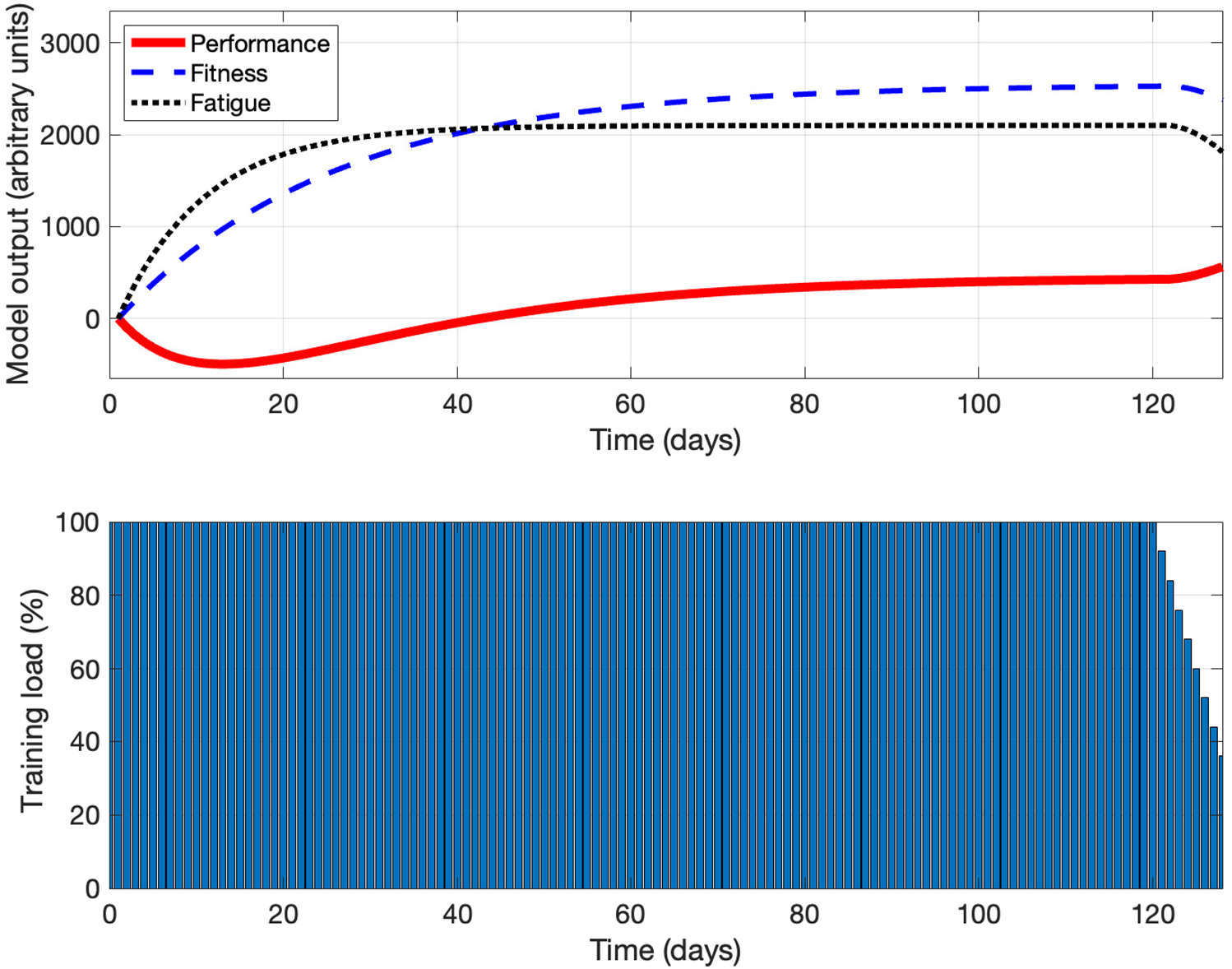
Figure 1: The simulation results without using optimal control theory

In the three simulation experiments with using optimal control theory, tp and A in Eq. (4) are set as tp=128 days and A=0.0003. In order to understand the effects of limiting the lower bound of w(t) during solving the proposed optimal control framework, M1 is set as 0, 20 and 40, respectively, while M2 is set as a constant 100; in other words, in these three simulation experiments, the range of w(t) is set as 0≤w(t)≤100, 20≤w(t)≤100 and 40≤w(t)≤100, respectively. Each simulation experiment with using optimal control theory is performed using the solution methods described in the Section 2.2 to obtain the optimal performance, fitness, fatigue and training load over time from the initial day to the competition day. Two metrics, the performance on the competition day and the cumulative training load during the training course, are specifically recorded.

To understand whether the proposed optimal control framework can design an optimal training program that can maximize the performance on the competition day and minimize the cumulative training load during the training course, we descriptively compare these two metrics generated by training programs with and without using optimal control theory.

3  Results and Discussion

Fig. 1 shows the simulation results without using optimal control theory. From this figure, we can understand how performance, fitness, fatigue and training load change over time during the training course until the competition day, and understand the relationship between these variables. It can be observed that, in the early stages of training, performance decreases since fatigue outweighs fitness; it is probably because the athlete just begins to adapt to training, therefore fatigue increases significantly. As training progresses, fitness continues to increase significantly while fatigue just increases slightly, leading to improved performance. Most notably, as the training load starts to decrease after the 120th day, performance starts to improve significantly, suggesting that reducing the training load at a certain time during the training course before the competition day could be beneficial for improving performance.

Fig. 2 shows the simulation results with using optimal control theory with 0≤w(t)≤100. It can be observed that both fatigue and fitness increase synchronously as training load increases; however, fatigue outweighs fitness slightly, causing performance to decrease slightly. As the training load reaches the highest value, fatigue starts to decrease and fitness starts to outweigh fatigue; as a result, performance starts to improve. This pattern is similar to that in Fig. 1. As the training load starts to decrease after the 114th day, performance starts to improve significantly and then reaches the highest value exactly on the competition day.

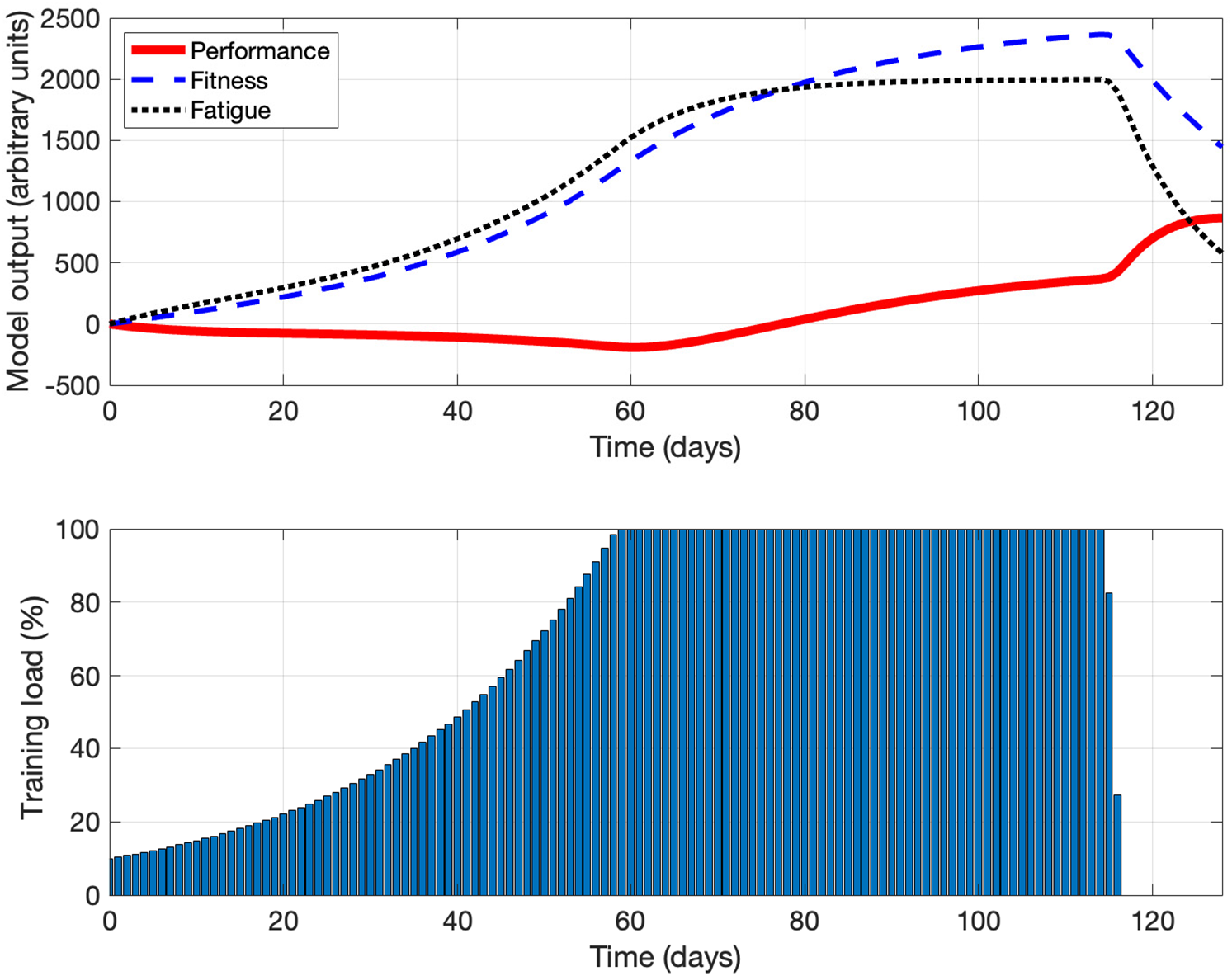
Figure 2: The simulation results using optimal control theory with 0≤w(t)≤100

The results of Figs. 1 and 2 provide an important clue that strategically reducing the training load at a certain time during the training course could be beneficial to improve performance significantly. It suggests that, the focus of an optimal training program should not always be on pushing an athlete to train more and harder, but should be on helping an athlete seek an optimal balance between training and recovery; an optimal training program should carefully consider both the intensity of training and an athlete’s ability and need for recovery to optimize performance effectively.

Figs. 3 and 4 show the results of the simulation experiments using optimal control theory with 20≤w(t)≤100 and 40≤w(t)≤100, respectively. By comparing the results of Figs. 2–4, we can understand how setting the lower bound of w(t) (i.e., the minimum daily training load during the training course) could affect the performance on the competition day. It can be observed that, the patterns of performance, fitness, fatigue, as well as the values of the performance on the competition day and the cumulative training load during the training course, are completely different between the experiments without (Fig. 2) and with (Figs. 3 and 4) setting the lower bound of w(t). In each of these experiments, performance reaches the highest value exactly on the competition day; however, the lower the lower bound of w(t), the higher the highest performance.

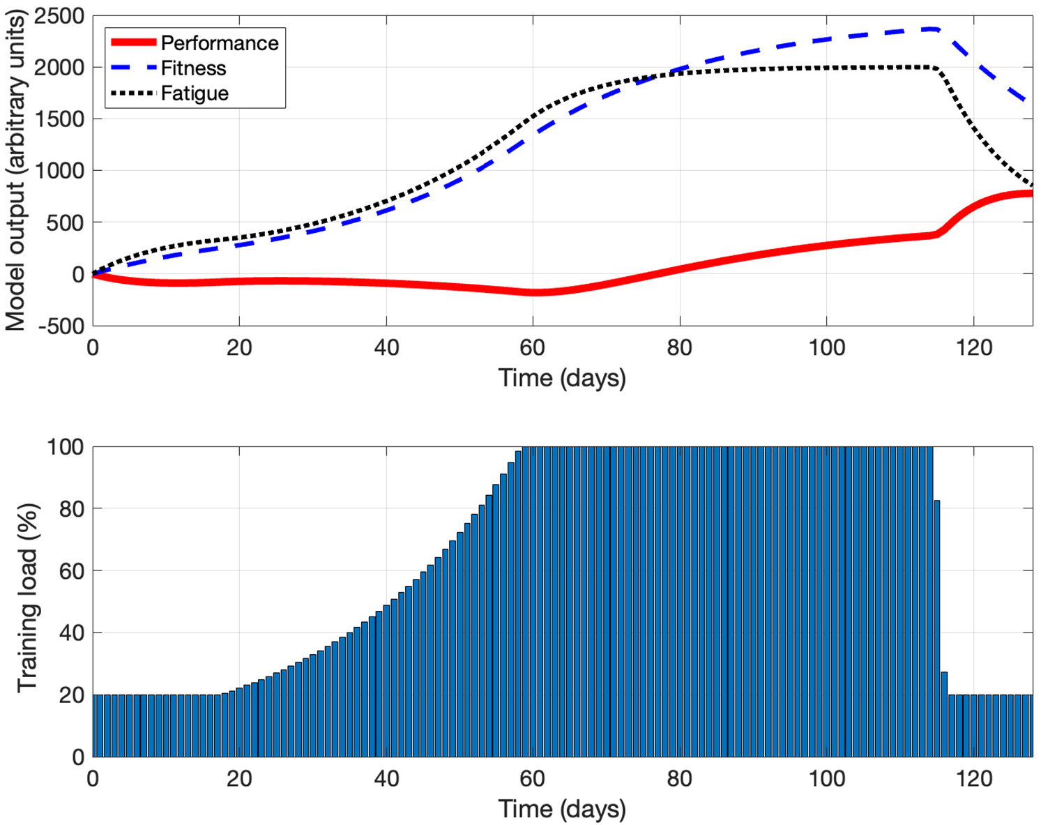
Figure 3: The simulation results using optimal control theory with 20≤w(t)≤100

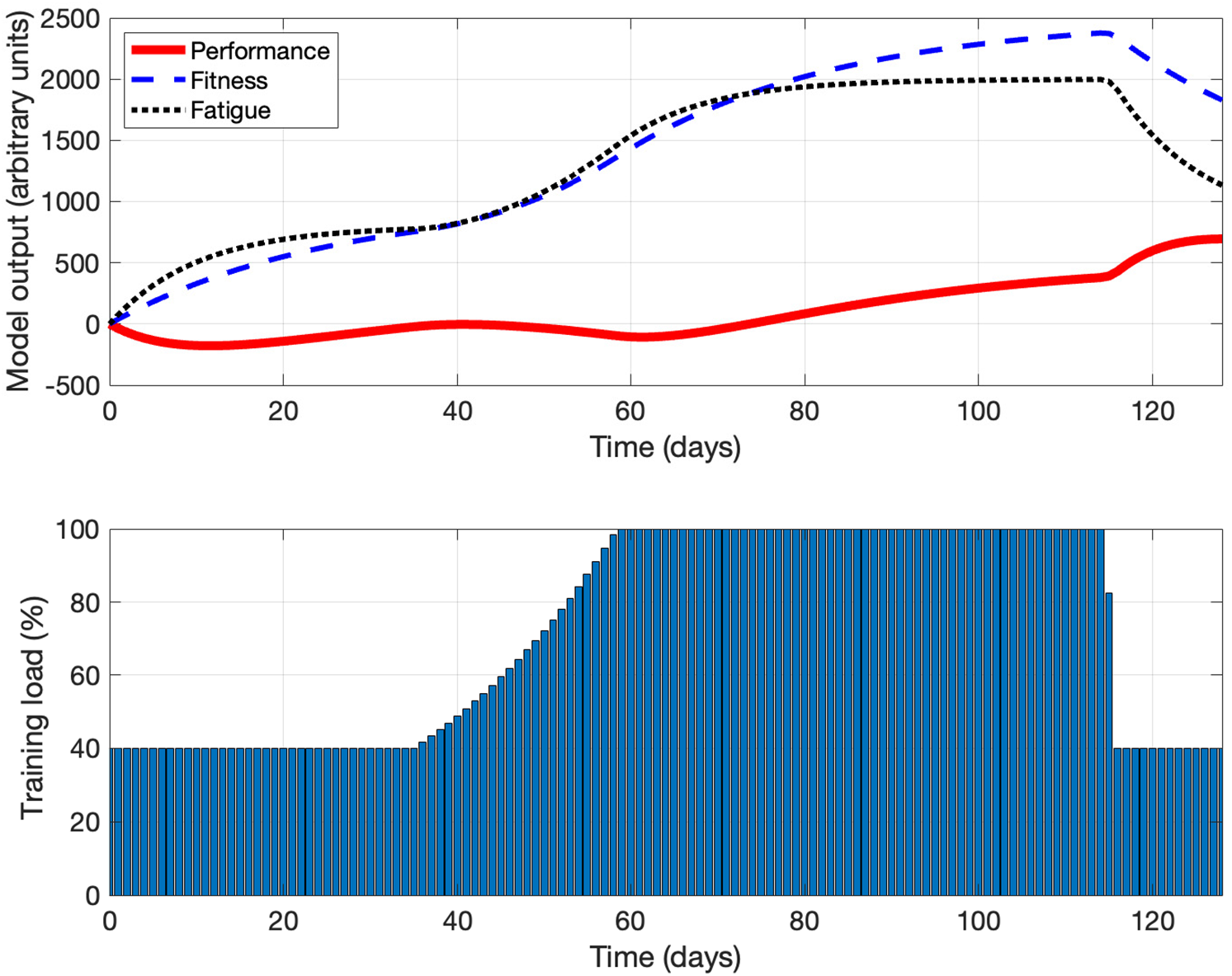
Figure 4: The simulation results using optimal control theory with 40≤w(t)≤100

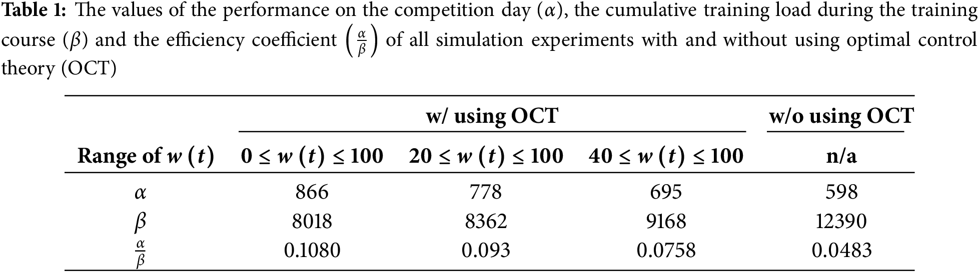
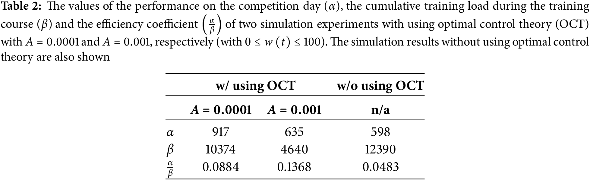
The values of the performance on the competition day and the cumulative training load during the training course of all simulation experiments are summarized in Table 1. It can be observed that, in each experiment with using optimal control theory, the performance on the competition day is higher while the cumulative training load during the training course is lower than those in the experiment without using optimal control theory, showing the feasibility and benefits of using the proposed optimal control framework to design optimal training programs for helping athletes achieve the best performance exactly on the competition day while properly manage training load during the training course for preventing overtraining. If the efficiency coefficient is defined as the performance on the competition day over the cumulative training load during the training course as shown in Table 1, it can be observed that the experiment with using optimal control theory with 0≤w(t)≤100 has the highest efficiency while the experiment without using optimal control theory has the lowest efficiency. In the three experiments with using optimal control theory, the lower the lower bound of w(t), the higher the efficiency, and this finding suggests that the proposed optimal control framework without limiting the lower bound of w(t) can design the best and most efficient optimal training program that maximizes the performance on the competition day while minimizes the cumulative training load during the training course.

The simulation results show that the performance on the competition day with using optimal control theory (with 0≤w(t)≤100) is 44.82% higher than that without. However, it is important to note that these simulation results are derived from the parameters of an individual athlete. Since the efficacy of an optimal training program designed using the proposed optimal control framework should be dependent on the physiological characteristics of an athlete, it may not always be that high for all athletes. For example, for the simulation results derived from another set of parameters that represents another athlete shown in Section 3 of the supplementary material, the performance on the competition day with using optimal control theory (with 0≤w(t)≤100) is only 3.38% higher than that without. However, it is important to note that, in competitive sports especially at the elite level, even a small change in performance can have substantial effects on an athlete’s chance of winning or medaling [45–48], and this small but significant change that can have drastic effects on the outcome of a sporting event is often less than 1% or 2% [49,50]. Hence, the proposed optimal control framework is flexible, could work well for different athletes with different physiological characteristics and personal goals.

It is important to discuss the effects and practical implications of the parameter A in Eq. (4). To understand the effects and practical implications of the parameter A, it is first necessary to note that if w(t) has no upper bound, the profile of an optimal w(t) (denoted as w∗(t) below) solved by the proposed optimal control framework looks as shown in Fig. 5. The effects of A is on determining the range and maximum of w∗(t); the lower the value of A, the larger the maximum of w∗(t). For example, Fig. 5 is a w∗(t) designed using A=1, and it can be observed that the maximum of this w∗(t) is around 0.1026. Figs. 6 and 7 show two w∗(t) designed using A=0.1 and A=0.01, respectively, and it can be observed that the maximums of these two w∗(t) are higher than the maximum of w∗(t) designed using A=1. Hence, since the range of w(t) is defined between 0 and 100 in the proposed optimal control framework as Eq. (7) shows, it is necessary to properly set the value of A before solving the proposed optimal control framework such that the range of a w∗(t) is between 0 and 100. Since the upper bound of w(t) is set as 100 during the solving process of the proposed optimal control framework, the maximum of a w∗(t) must be limited to 100 or under; as a result, the profile of a w∗(t) could look like the one designed using A=0.0001 as shown in Fig. 8. Since the physical meaning of w∗(t) is an optimal training program (that indicates the optimal magnitude of training load in each day during the training course) designed by the proposed optimal control framework, it can be interpreted that the practical implication of A is a parameter associated with the characteristics of an optimal training program, determining the value of the maximum daily training load and the number of days that an athlete trains with the maximum daily training load during the training course. In addition, since the characteristics of w∗(t) determines the performance on the competition day and the cumulative training load during the training course, the parameter that determines the characteristics of w∗(t), i.e., A, determines these effects of training. In using the proposed optimal control framework to design optimal training programs in real applications, one can freely set the value of A according to the purposes and expected results. For example, if the purpose is to achieve higher performance on the competition day, regardless of the cumulative training load during the training course, then one can design an optimal training program using A=0.0001 as shown in Fig. 8. On the other hand, if the purpose is to seek a balance between these two metrics, then one can design an optimal training program using A=0.001 as shown in Fig. 9. The simulation results of these two cases are shown in Table 2. It can be observed that the performance on the competition day with A=0.0001 is higher than that with A=0.001, but the cumulative training load of the former is higher than that of the latter.

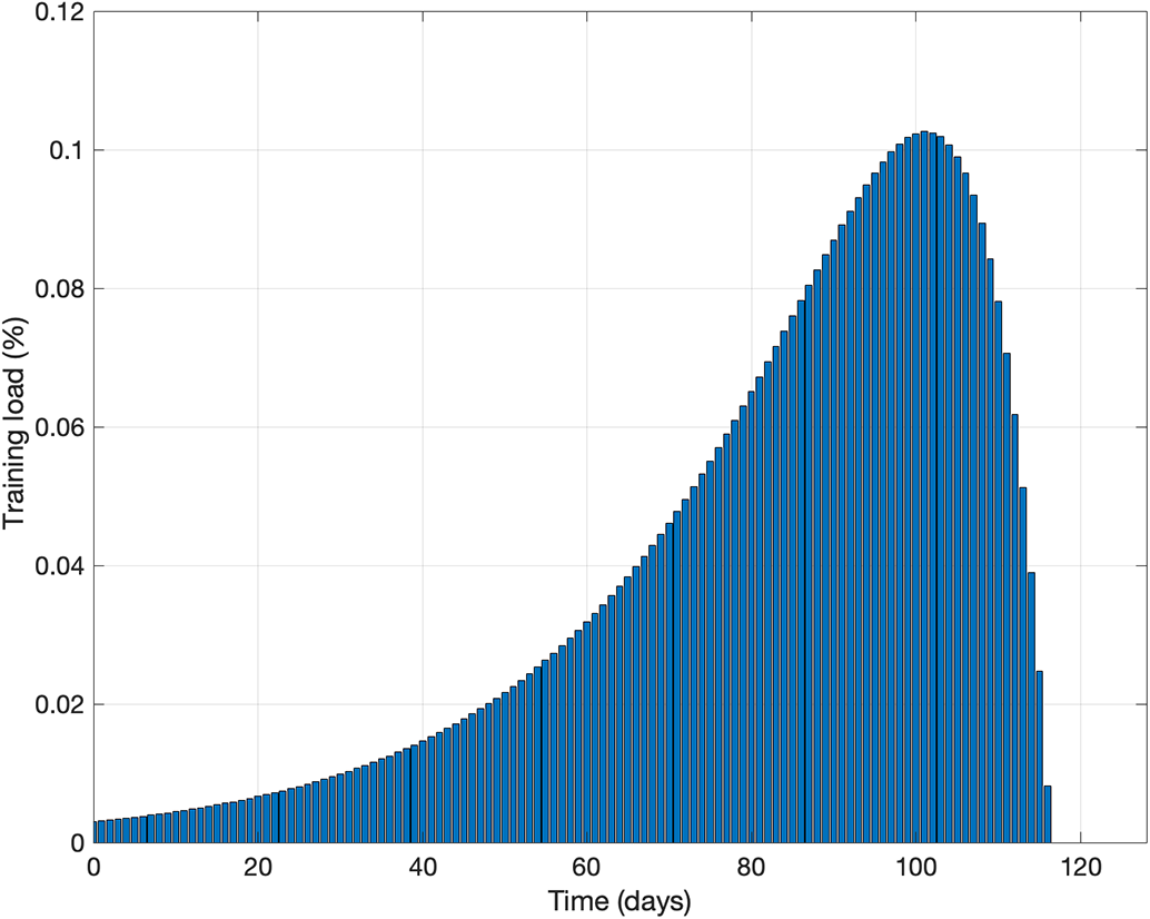
Figure 5: Illustration of a w∗(t) designed using A=1

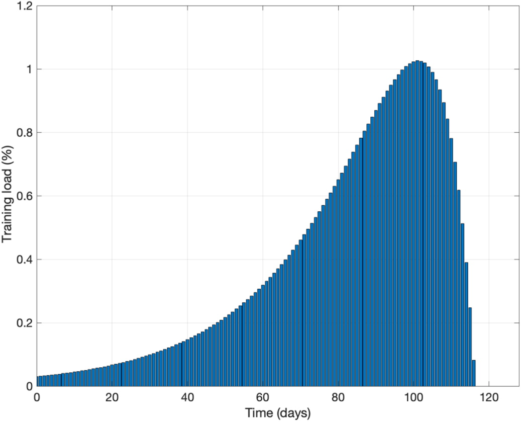
Figure 6: Illustration of a w∗(t) designed using A=0.1

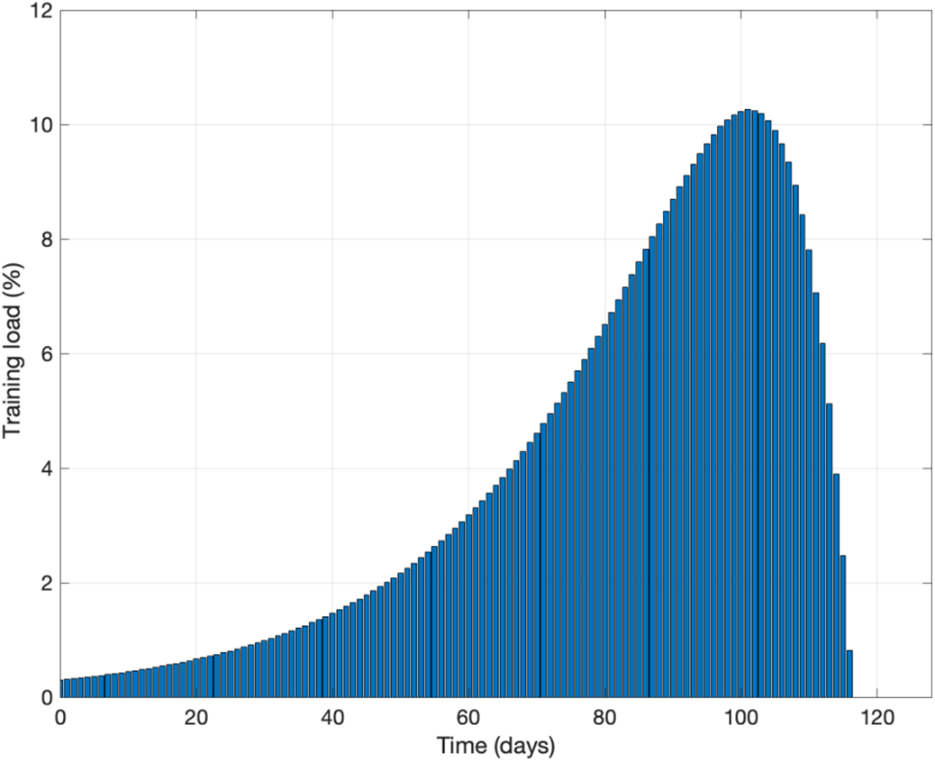
Figure 7: Illustration of a w∗(t) designed using A=0.01

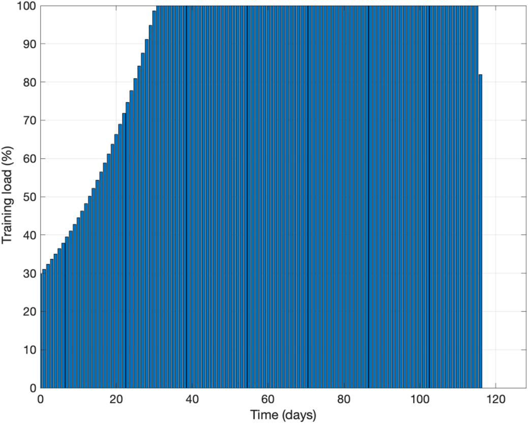
Figure 8: Illustration of a w∗(t) designed using A=0.0001

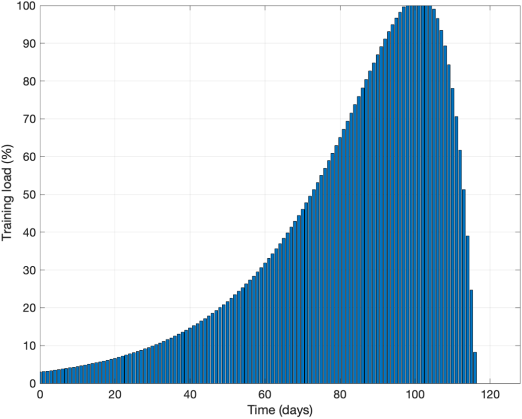
Figure 9: Illustration of a w∗(t) designed using A=0.001

The main limitations of the present study are related to the assumptions of the training-performance model, i.e., Eq. (2), used in the proposed optimal control framework. First, this model is an empirical (or say phenomenological) model formulated based on empirical concepts and observations, but not a mechanistic model that takes underlying mechanisms into account; in other words, this model only considers the overall positive and negative effects on performance (i.e., fitness and fatigue in the model, respectively), but does not consider the individual effect of every possible factor that could affect performance. Second, in this model, the dynamical response of fitness or fatigue that contributes to the change of performance is assumed to be a first-order linear differential equation, but this mathematical form could be too simple to accurately describe the complicated relationship between training and performance; to address this issue, several modified models based on the original Banister IR model with more elaborate mathematical forms have subsequently been proposed to improve the descriptive and predictive abilities of the models [9–13]. Third, this model does not consider physiological adaptions to training; that is, the coefficients (i.e., τ1, τ2, k1 and k2) in Eq. (2) that represent the physiological characteristics of an athlete are assumed to be time-invariant constants; however, in reality, the physiological characteristics of an athlete could adapt to training and change over time, therefore it could be more reasonable to model these coefficients as functions of time [1,3,4]. In summary, as a pilot study that intends to develop a novel method by the combined use of optimal control theory and a training-performance model for designing optimal training programs, we choose to adopt a model with a simpler mathematical form to formulate the proposed optimal control framework, such that the proposed optimal control framework can be easier to formulate and solve, facilitating us to assess the feasibility of this innovative idea as well as to demonstrate the existence and uniqueness of the optimal solutions. In the future, it is necessary to adopt a more advanced training-performance model (rather than the earliest and simplest Banister IR model) to formulate the optimal control framework. Furthermore, in the future, experiments are needed to justify whether a designed optimal training program using the proposed optimal control framework is indeed optimal, and whether it can help athletes achieve the best performance exactly on the competition day while properly manage training load during the training course to prevent overtraining.

4  Conclusions

To the best of our knowledge, it is the first study that intends to develop a novel method by the combined use of optimal control theory and a training-performance model for designing optimal training programs that can be served as references for coaches, trainers and athletes to design training programs, to help athletes achieve the best performance exactly on the competition day while properly manage training load during the training course for preventing overtraining. Specifically speaking, the function of the proposed optimal control framework is to, based on the physiological characteristics of an athlete and the personal goals, design an optimal training program that indicates the ideal magnitude of training load on each day during the training course until the competition day. Coaches, trainers, and the athlete can then refer to this optimal suggestion to design the daily training load of a training program to help the athlete achieve the best performance exactly on the competition day while properly manage training load during the training course to prevent overtraining. The simulation results show that the performance on the competition day is higher while the cumulative training load during the training course is lower with using optimal control theory than those without, successfully showing the feasibility and benefits of using the proposed optimal control framework to design optimal training programs for helping athletes achieve the best performance exactly on the competition day while properly manage training load during the training course for preventing overtraining. In addition, an optimal training program designed by the proposed optimal control framework can be personalized to match the physiological characteristics and personal goals of an athlete; therefore, the proposed optimal control framework is flexible, could work well for different athletes with different physiological characteristics and personal goals. The present feasibility study lays the foundation of the combined use of optimal control theory and training-performance models to design personalized optimal training programs in real applications in athletic training and sports science for helping athletes achieve the best performances in competitions while prevent overtraining and the risk of overuse injuries. The main limitation of the present study is that the training-performance model adopted to formulate the optimal control framework could be too simple to accurately and realistically describe the dynamics of performance and training load. In the future, it is necessary to adopt a more advanced training-performance model (rather than the earliest and simplest Banister IR model) to formulate the optimal control framework.

Acknowledgement: Not applicable.

Funding Statement: This research was funded by the National Science and Technology Council, grant number NSTC 113-2221-E-002-136-.

Author Contributions: Conceptualization, Yi Yang and Che-Yu Lin; methodology, Yi Yang and Che-Yu Lin; software, Yi Yang; validation, Yi Yang; formal analysis, Yi Yang and Che-Yu Lin; investigation, Yi Yang and Che-Yu Lin; resources, Che-Yu Lin; writing—original draft preparation, Yi Yang and Che-Yu Lin; writing—review and editing, Yi Yang and Che-Yu Lin; visualization, Yi Yang and Che-Yu Lin; supervision, Che-Yu Lin; project administration, Che-Yu Lin; funding acquisition, Che-Yu Lin. All authors reviewed the results and approved the final version of the manuscript.

Availability of Data and Materials: Please find the supplementary data for all of the raw data used for producing all of the results, figures and tables relevant to this study.

Ethics Approval: Not applicable.

Conflicts of Interest: The authors declare no conflicts of interest to report regarding the present study.

Supplementary Materials: The supplementary material is available online at https://www.techscience.com/doi/10.32604/cmes.2025.064459/s1.

References

1. Borresen J, Lambert MI. The quantification of training load, the training response and the effect on performance. Sports Med. 2009;39:779–95. doi:10.2165/11317780-000000000-00000. [Google Scholar] [PubMed] [CrossRef]

2. Durell DL, Pujol TJ, Arnes JT. A survey of the scientific data and training methods utilized by collegiate strength and conditioning coaches. J Strength Cond Res. 2003;17(2):368–73. doi:10.1519/00124278-200305000-00026. [Google Scholar] [CrossRef]

3. Clarke DC, Skiba PF. Rationale and resources for teaching the mathematical modeling of athletic training and performance. Adv Physiol Educ. 2013;37(2):134–52. doi:10.1152/advan.00078.2011. [Google Scholar] [PubMed] [CrossRef]

4. Imbach F, Sutton-Charani N, Montmain J, Candau R, Perrey S. The use of fitness-fatigue models for sport performance modelling: conceptual issues and contributions from machine-learning. Sports Med-Open. 2022;8(1):29. doi:10.1186/s40798-022-00426-x. [Google Scholar] [PubMed] [CrossRef]

5. Taha T, Thomas SG. Systems modelling of the relationship between training and performance. Sports Med. 2003;33:1061–73. doi:10.2165/00007256-200333140-00003. [Google Scholar] [PubMed] [CrossRef]

6. Busso T, Thomas L. Using mathematical modeling in training planning. Int J Sports Physiol Perform. 2006;1(4):400–5. doi:10.1123/ijspp.1.4.400. [Google Scholar] [PubMed] [CrossRef]

7. Banister EW, Calvert TW, Savage MV, Bach T. A systems model of training for athletic performance. Aust J Sports Med. 1975;7(3):57–61. [Google Scholar]

8. Calvert TW, Banister EW, Savage MV, Bach T. A systems model of the effects of training on physical performance. IEEE Trans Syst Man Cybern Syst. 1976;2:94–102. doi:10.1109/TSMC.1976.5409179. [Google Scholar] [CrossRef]

9. Busso T. Variable dose-response relationship between exercise training and performance. Med Sci Sports Exerc. 2003;35(7):1188–95. doi:10.1249/01.MSS.0000074465.13621.37. [Google Scholar] [PubMed] [CrossRef]

10. Hellard P, Avalos M, Millet G, Lacoste L, Barale F, Chatard JC. Modeling the residual effects and threshold saturation of training: a case study of olympic swimmers. J Strength Cond Res. 2005;19(1):67–75. doi:10.1519/00124278-200502000-00012. [Google Scholar] [CrossRef]

11. Busso T. From an indirect response pharmacodynamic model towards a secondary signal model of dose-response relationship between exercise training and physical performance. Sci Rep. 2017;7(1):40422. doi:10.1038/srep40422. [Google Scholar] [PubMed] [CrossRef]

12. Kolossa D, Azhar B, Rasche C, Endler S, Hanakam F, Ferrauti A, et al. Performance estimation using the fitness-fatigue model with Kalman filter feedback. Int J Comput Sci Sport. 2017;16(2):117–29. doi:10.1515/ijcss-2017-0010. [Google Scholar] [CrossRef]

13. Turner JD, Mazzoleni MJ, Little JA, Sequeira D, Mann BP. A nonlinear model for the characterization and optimization of athletic training and performance. Biomed Hum Kinet. 2017;9(1):82–93. doi:10.1515/bhk-2017-0013. [Google Scholar] [CrossRef]

14. Couceiro MS, Dias G, Araújo D, Davids K. The ARCANE project: how an ecological dynamics framework can enhance performance assessment and prediction in football. Sports Med. 2016;46(12):1781–6. doi:10.1007/s40279-016-0549-2. [Google Scholar] [PubMed] [CrossRef]

15. Den Hartigh RJ, Meerhoff LRA, Van Yperen NW, Brauers JJ, Frencken WG, Emerencia A, et al. Resilience in sports: a multidisciplinary, dynamic, and personalized perspective. Int Rev Sport Exerc Psychol. 2024;17(1):564–86. doi:10.1080/1750984X.2022.2039749. [Google Scholar] [PubMed] [CrossRef]

16. Kirk DE. Optimal control theory: an introduction. Chelmsford, MA, USA: Courier Corporation; 2012. [Google Scholar]

17. Macki J, Strauss A. Introduction to optimal control theory. New York, NY, USA: Springer; 2012. [Google Scholar]

18. Hull DG. Optimal control theory for applications. New York, NY, USA: Springer; 2013. [Google Scholar]

19. Ma Z, Zou S. Optimal control theory. Singapore: Springer; 2021. [Google Scholar]

20. Sethi SP. Optimal control theory: applications to management science and economics. New York, NY, USA: Springer; 2021. [Google Scholar]

21. Razavi SE, Moradi MA, Shamaghdari S, Menhaj MB. Adaptive optimal control of unknown discrete-time linear systems with guaranteed prescribed degree of stability using reinforcement learning. Int J Dyn Control. 2022;10(3):870–8. doi:10.1007/s40435-021-00836-x. [Google Scholar] [CrossRef]

22. Chen X, Jin T. Optimal control for a multistage uncertain random system. IEEE Access. 2023;11:2105–17. doi:10.1109/ACCESS.2023.3234068. [Google Scholar] [CrossRef]

23. Hou LF, Li L, Chang L, Wang Z, Sun GQ. Pattern dynamics of vegetation based on optimal control theory. Nonlinear Dyn. 2025;113(1):1–23. doi:10.1007/s11071-024-10241-6. [Google Scholar] [CrossRef]

24. Jin C, Mao H, Chen Y, Shi Q, Wang Q, Ma G, et al. Engineering-oriented dynamic optimal control of a greenhouse environment using an improved genetic algorithm with engineering constraint rules. Comput Electron Agric. 2020;177:105698. doi:10.1016/j.compag.2020.105698. [Google Scholar] [CrossRef]

25. Hamelin FM, Bowen B, Bernhard P, Bokil VA. Optimal control of plant disease epidemics with clean seed usage. Bull Math Biol. 2021;83:1–24. doi:10.1007/s11538-021-00872-w. [Google Scholar] [PubMed] [CrossRef]

26. Luiz MHR, Takahashi LT, Bassanezi RC. Optimal control in citrus diseases. Comput Appl Math. 2021;40(6):191. doi:10.1007/s40314-021-01581-9. [Google Scholar] [CrossRef]

27. Ali HM, Ameen IG. Stability and optimal control analysis for studying the transmission dynamics of a fractional-order MSV epidemic model. J Comput Appl Math. 2023;434(3):115352. doi:10.1016/j.cam.2023.115352. [Google Scholar] [CrossRef]

28. Kadakia N. Optimal control methods for nonlinear parameter estimation in biophysical neuron models. PLoS Comput Biol. 2022;18(9):e1010479. doi:10.1371/journal.pcbi.1010479. [Google Scholar] [PubMed] [CrossRef]

29. Libotte GB, Lobato FS, Platt GM, Neto AJS. Determination of an optimal control strategy for vaccine administration in COVID-19 pandemic treatment. Comput Methods Programs Biomed. 2020;196:105664. doi:10.1016/j.cmpb.2020.105664. [Google Scholar] [PubMed] [CrossRef]

30. Nana-Kyere S, Boateng FA, Jonathan P, Donkor A, Hoggar GK, Titus BD, et al. Global analysis and optimal control Model of COVID-19. Comput Math Methods Med. 2022;2022(1):9491847. doi:10.1155/2022/9491847. [Google Scholar] [PubMed] [CrossRef]

31. Shindi O, Kanesan J, Kendall G, Ramanathan A. The combined effect of optimal control and swarm intelligence on optimization of cancer chemotherapy. Comput Methods Programs Biomed. 2020;189:105327. doi:10.1016/j.cmpb.2020.105327. [Google Scholar] [PubMed] [CrossRef]

32. Blueschke D, Savin I, Blueschke-Nikolaeva V. An evolutionary approach to passive learning in optimal control problems. Comput Econ. 2020;56(3):659–73. doi:10.1007/s10614-019-09961-4. [Google Scholar] [PubMed] [CrossRef]

33. Liang Y, Zhang WH, Lu Y, Wang ZS. Optimal control and Simulation for enterprise financial risk in Industry environment. Math Probl Eng. 2020;2020(1):6040597. doi:10.1155/2020/6040597. [Google Scholar] [CrossRef]

34. Shekhar C, Varshney S, Kumar A. Optimal control of a service system with emergency vacation using bat algorithm. J Comput Appl Math. 2020;364:112332. doi:10.1016/j.cam.2019.06.048. [Google Scholar] [CrossRef]

35. Rarità L, Stamova I, Tomasiello S. Numerical schemes and genetic algorithms for the optimal control of a continuous model of supply chains. Appl Math Comput. 2021;388:125464. doi:10.1016/j.amc.2020.125464. [Google Scholar] [CrossRef]

36. Luo W, Yuan D, Jin D, Lu P, Chen J. Optimal control of slurry pressure during shield tunnelling based on random forest and particle swarm optimization. Comput Model Eng Sci. 2021;128(1):109–27. doi:10.32604/cmes.2021.015683. [Google Scholar] [CrossRef]

37. Yoo H, Kim B, Kim JW, Lee JH. Reinforcement learning based optimal control of batch processes using Monte-Carlo deep deterministic policy gradient with phase segmentation. Comput Chem Eng. 2021;144(4):107133. doi:10.1016/j.compchemeng.2020.107133. [Google Scholar] [CrossRef]

38. Zhao L, Huang Z, Fu Q, Fang N, Xing B, Chen J. HVAC optimal control based on the sensitivity analysis: an improved SA combination method based on a neural network. Comput Model Eng Sci. 2023;136(3):2741–58. doi:10.32604/cmes.2023.025500. [Google Scholar] [CrossRef]

39. Imran M, McKinney B, Butt AIK. SEIR mathematical model for Influenza-Corona co-infection with treatment and hospitalization compartments and optimal control strategies. Comput Model Eng Sci. 2025;142(2):1899–1931. doi:10.32604/cmes.2024.059552. [Google Scholar] [CrossRef]

40. Abidemi A, Aziz NAB. Optimal control strategies for dengue fever spread in Johor. Malaysia Comput Methods Programs Biomed. 2020;196:105585. doi:10.1016/j.cmpb.2020.105585. [Google Scholar] [PubMed] [CrossRef]

41. Zouhri S, El Baroudi M, Saadi S. Optimal control with isoperimetric constraint for chemotherapy of tumors. Int J Appl Comput Math. 2022;8(4):215. doi:10.1007/s40819-022-01425-y. [Google Scholar] [CrossRef]

42. El Baroudi M, Laarabi H, Zouhri S, Rachik M, Abta A. Stochastic optimal control model for COVID-19: mask wearing and active screening/testing. J Appl Math Comput. 2024;70:6411–41. doi:10.1007/s12190-024-02220-2. [Google Scholar] [CrossRef]

43. Tassé AJO, Kubalasa VB, Tsanou B. Nonstandard finite difference schemes for some epidemic optimal control problems. Math Comput Simul. 2025;228:1–22. doi:10.1016/j.matcom.2024.08.028. [Google Scholar] [CrossRef]

44. Lenhart S, Workman JT. Optimal control applied to biological models. Boca Raton, FL, USA: Chapman and Hall/CRC; 2007. [Google Scholar]

45. Pyne DB, Hopkins WG, Batterham AM, Gleeson M, Fricker PA. Characterising the individual performance responses to mild illness in international swimmers. Br J Sports Med. 2005;39(10):752–6. doi:10.1136/bjsm.2004.017475. [Google Scholar] [PubMed] [CrossRef]

46. Bradshaw EJ, Hume PA, Aisbett B. Performance score variation between days at Australian national and Olympic women’s artistic gymnastics competition. J Sports Sci. 2012;30(2):191–9. doi:10.1080/02640414.2011.633927. [Google Scholar] [PubMed] [CrossRef]

47. Lim JJ, Kong PW. Effects of isometric and dynamic postactivation potentiation protocols on maximal sprint performance. J Strength Cond Res. 2013;27(10):2730–6. doi:10.1519/jsc.0b013e3182815995. [Google Scholar] [PubMed] [CrossRef]

48. Park JL, Fairweather MM, Donaldson DI. Making the case for mobile cognition: eEG and sports performance. Neurosci Biobehav Rev. 2015;52:117–30. doi:10.1016/j.neubiorev.2015.02.014. [Google Scholar] [PubMed] [CrossRef]

49. Currell K, Jeukendrup AE. Validity, reliability and sensitivity of measures of sporting performance. Sports Med. 2008;38:297–316. doi:10.2165/00007256-200838040-00003. [Google Scholar] [PubMed] [CrossRef]

50. Bellar D, LeBlanc NR, Campbell B. The effect of 6 days of alpha glycerylphosphorylcholine on isometric strength. J Int Soc Sports Nutr. 2015;12(1):1–6. doi:10.1186/s12970-015-0103-x. [Google Scholar] [PubMed] [CrossRef]