Fusion Prototypical Network for 3D Scene Graph Prediction

1  Introduction

The concept of scene graphs, initially introduced for 2D images [1–4], has been adapted for 3D environments to enhance scene understanding in various applications such as virtual reality [5–8], augmented reality [9–11], and autonomous navigation [12–14]. The shift from 2D to 3D involves additional challenges, such as needing to interpret accurately the spatial relationships and volumetric properties of objects, which are more complex in a three-dimenmsional context.

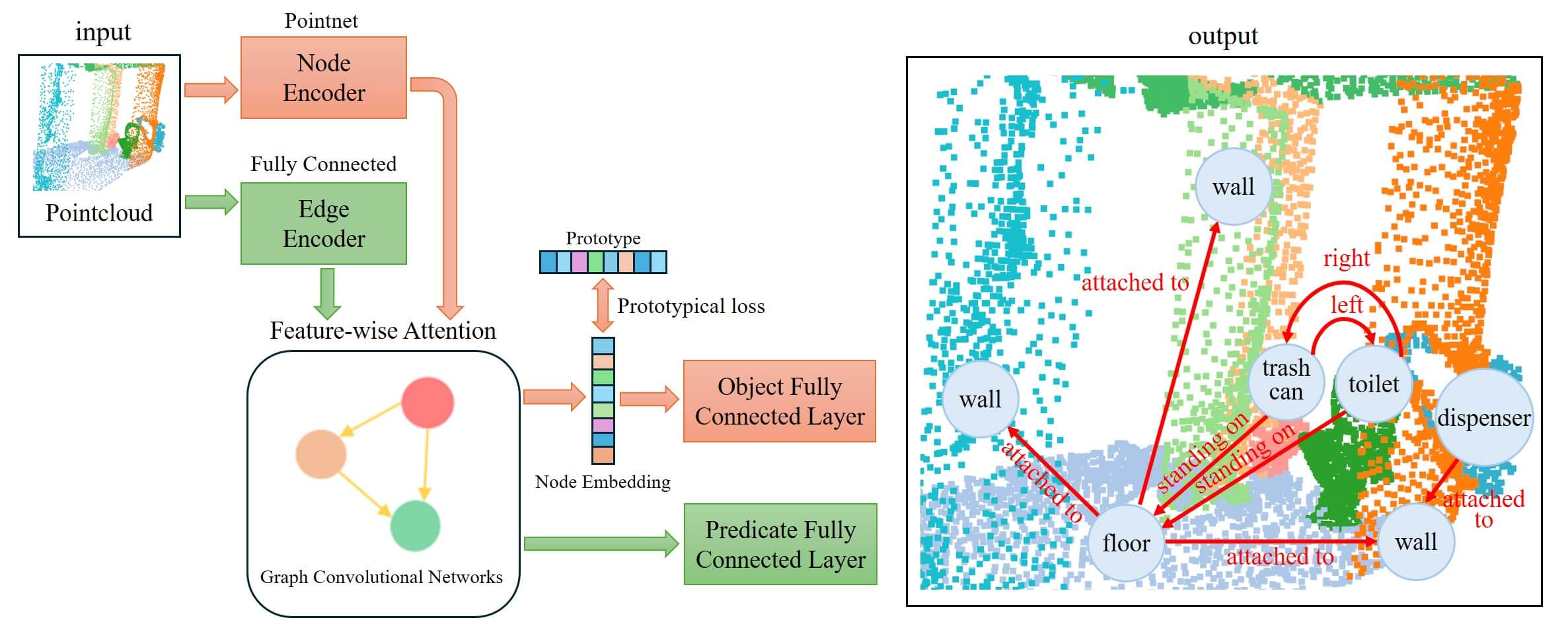
3D semantic scene graph (3DSSG) [15] has made significant contributions to the problem of scene graph prediction in 3D indoor environments. 3DSSG proposed a 3D semantic scene graph dataset based on the 3RScan dataset [16] and utilized it to demonstrate remarkable performance through a scene graph prediction network (SGPN) [15]. Since then, most researchers have proposed scene-graph prediction models based on SGPN. Fig. 1 shows the structure of a typical scene-graph prediction model. After 3DSSG, most researchers improved the model’s performance by changing each module, such as the encoder, feature input, and graph reasoning using various method. Most studies employed Pointnet as the encoder [15,17], and some used either a dynamic graph convolutional neural network [18,19] or point transformers [20,21]. Feature input initially uses a masked point cloud per instance [15,22], and later adds geometric information or statistical metrics such as mean, variance [23,24]. Graph reasoning initially used graph convolutional networks (GCN) [15,25], and later used various GCN-based attention [26] models, such as EdgeGCN, feature wise attention (FAT), to better capture features [19,23]. Recent studies have mainly improved performance by adding visual and linguistic information to existing models. They integrated 3D point clouds with 2D images [24,27] and language-based models like contrastive language-image pretraining (CLIP) or a large language model (LLM) [24,27–30].

Figure 1: Typical 3D scene graph prediction structure

In the 3DSSG dataset, both objects and predicates exhibited extremely long-tail distribution. In particular, objects had 160 classes,of which approximately 50 had 10 or fewer data points. Despite these distributions for objects, most studies have focused on the long-tailed problem for predicates. Also, classes with 10 or fewer data elements occur more frequently in few-shot learning than general deep learning tests. In this paper, we present a fusion prototypical network (FPN) that approaches sparse classes in data as few-shot learning and rich data as general deep learning. To achieve this, the embedding space of the graph reasoning output is altered by utilizing prototypical loss with the intention of optimally inducing the classifier to capture sparse classes. We quantitatively and qualitatively evaluated the proposed method on the 3DSSG dataset and found that it improved the performance of sparse classes.

2  Related Work

2.1 Scene Graph Prediction: The Point Cloud Approach

Image-based scene graph prediction is an extensively researched field, with notable advancements in modeling semantic relationships between objects within images. However, there has also been a recent surge in research on 3D-based scene graph prediction using point clouds. Table 1 shows a comparative analysis of the 3D scene graph prediction models. The pioneering work in 3D scene graph prediction is from the 3DSSG framework [15], which introduced the 3DSSG generation dataset leveraging the 3RScan dataset and a neural network named SGPN, which combines Graph Convolution Networks (GCNs) and PointNet [16]. The SGPN model utilizes GCNs to generate 3D graphs efficiently, but its performance is limited in environments with long-tail distributions. The SGGpoint model [19], developed by Zhang et al., employed an EdgeGCN to capture edge-based relationships within point clouds. Further improving the reasoning capabilities, Wu et al. [23] introduced the Scene Graph Fusion Network (SGFN), which sequentially generates 3D graphs from RGB-D sequences and integrates them through a Graph Fusion Attention (FAT) mechanism.

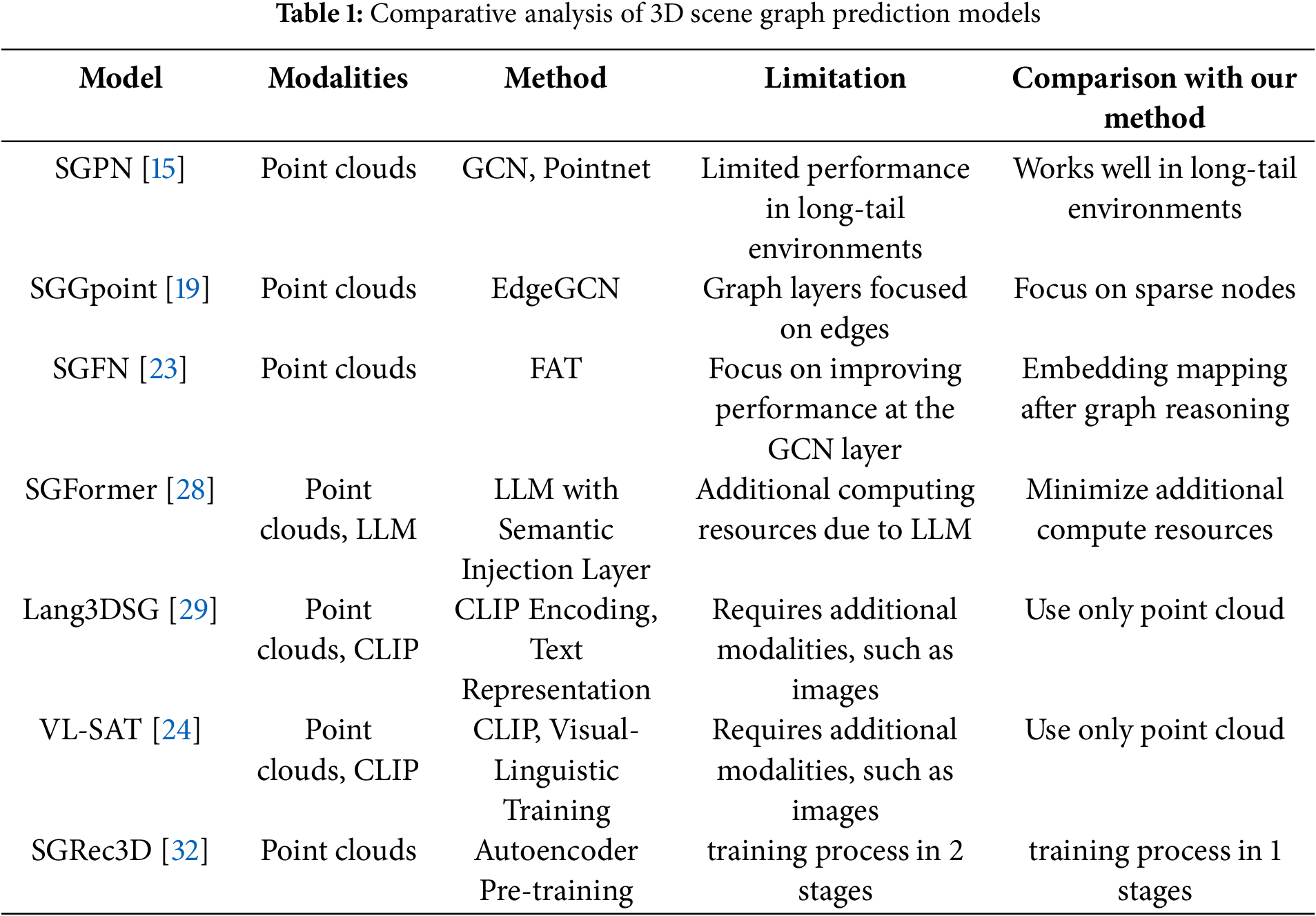
Knowledge-based research has also been conducted by scholars such as Zhang et al. [22] who proposed a knowledge-inspired network for embedding labels via meta-embedding and intervening features in scene graph prediction models. Feng et al. [31] used hierarchical symbolic knowledge to leverage external knowledge to improve the model’s classification performance for ambiguous relationships. The SGFormer [28] model employs an LLM to enhance the visual features of objects by leveraging knowledge from the semantic injection layer. Lang3DSG [29] inserted natural language information into the model by encoding objects and relationships as text using CLIP [30]. Similarly, visual-linguistic semantics-assisted training (VL-SAT) [24] overcomes the limitations of the existing point clouds by inserting natural language information through CLIP and using additional image data to provide visual information. These models require both point cloud and additional image modalities to improve performance, but their reliance on extra input data can be a limitation in real-world applications where only point cloud data may be available.

Meanwhile, SGRec3D [32] proposed a method for effectively training limited point-cloud data by using an autoencoder for pre-training.

2.2 Few-Shot Learning

Few-shot learning has recently garnered significant attention for training models with limited labeled data. One of the pioneering works in this domain is Matching Networks proposed by Vinyals et al. [33], which employs an attention mechanism to compare a small number of labeled examples with the query set, leveraging the concept of support and query samples to perform classification. Another notable approach is Prototypical Networks proposed by Snell et al. [34], which represents each class with a prototype, typically the mean of its support set, and classifies queries based on their proximity to these prototypes in the embedding space. Further advancements include model-agnostic meta-learning (MAML) by Finn et al. [35], which trains models to enable rapid adaptation to new tasks with few gradient steps. Sung et al. [36] improved the performance of relation networks in few-shot scenarios using a learnable deep distance metric to compute the similarities between samples. Recent work has also integrated transformer architectures, as seen in the few-Shot Transformer by Ye et al. [37], which captures long-range dependency and context. MetaOptNet by Lee et al. [38] combined optimization-based meta-learning with support set regularization to enhance the performance on standard benchmarks. Meanwhile, there is also a study that addresses the Few-Shot Class-Incremental Learning (FSCIL) problem by proposing a Filter Bank Network (FBN) [39], which augments learnable convolution filters instead of data, thereby effectively integrating new classes.

3  Proposed Method

Fig. 2 shows an overview of the proposed system which is similar to a typical scene-graph prediction model. However, we improve the model’s performance by changing the embedding space after applying graph reasoning. Section 3.1 presents a scene-graph prediction problem using the 3DSSG dataset. Section 3.2 describes the encoders for the nodes and edges and the GNN-based graph-reasoning method is explained in Section 3.3. Finally, the new, fusion prototypical loss learning method is detailed in Section 3.4.

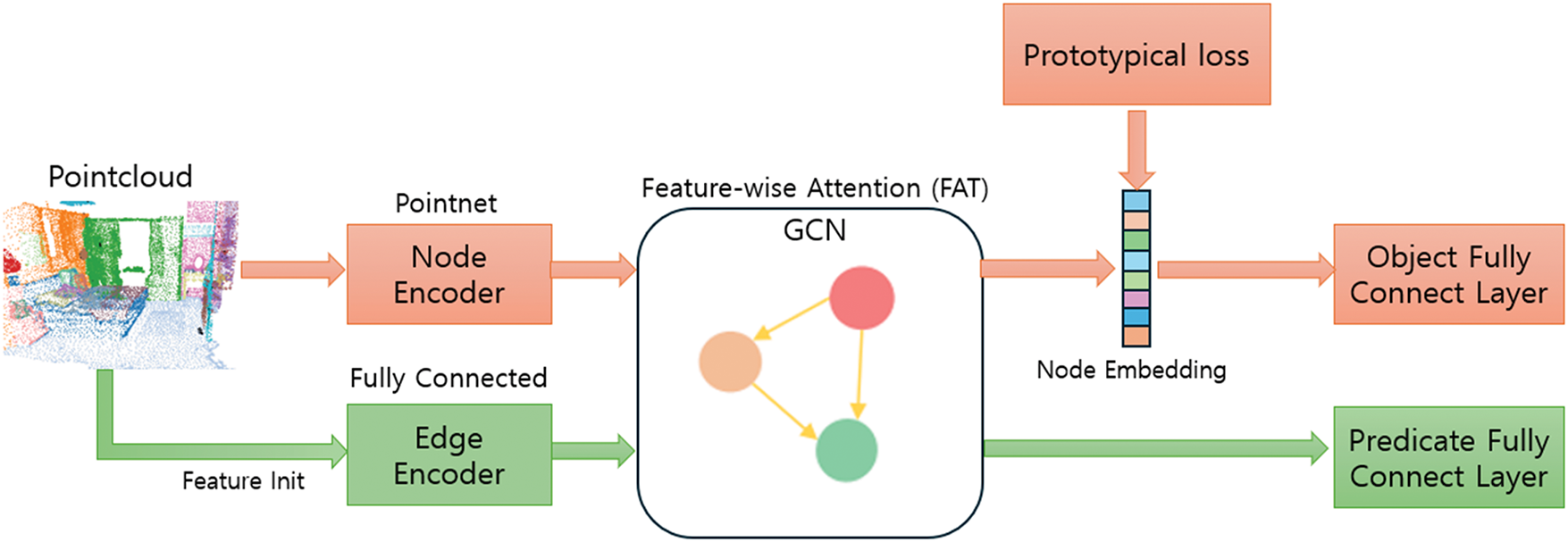
Figure 2: Overview of the proposed model

3.1 Problem Formulation

As input, we take a point cloud P∈RN×3 with N 3D points and with a set M∈{M1,M2,...,Mk} of k semantic instance masks described in 3DSSG [15]. We aim to generate a 3d semantic scene graph G={O,R}. The set of objects O={oi}i=1K represents the classification result of a point cloud P separated by a mask M. The set of relations R={rij}i,j represents the classification of predicates in a relational triple ⟨subject,predicate,object⟩ whose subject is oi and whose object is oj.

3.2 Encoder

The encoder comprises a Node Encoder for objects and an Edge Encoder for relations. Node Encoder extracts the initial node ϕo∈Rk×c and the Edge Encoder extracts the initial edge ϕr∈Rk×c. As input, the node encoder takes a semantic instance Pi∈RN×3 extracted using the mask mi∈M. We apply this to PointNet [17] to extract the features the point cloud, in the process extracting a c-dimensional representation of the object’s initial features ϕn.

The edge encoder uses the same approach as the SGFN [23]. It extracts various features between the semantic instance pi of subject and the semantic instance pj of object in the relational triple ⟨subject,predicate,object⟩ and passes them through the fully connected layer. Eq. (1) calculates the edge-encoding process. μ and σ are the mean and standard deviation of 3D points in each instance, respectively, b=(bx,by,bz) is the size, ν=bxbybz is the volumn, and l=max(bx,by,bz) is the maximum side length. cat(⋅) is concatenate and MLP(⋅) is fully connect layer. The initial edge feature, ϕr,ij, is the edge encoder’s output.

ϕr,ij=MLP(cat(μi−μj,σi−σj,bi−bj,lnlilj,lnνiνj))(1)

3.3 Graph Reasoning

For message propagation between the initial nodes ϕn and edges ϕr, we applied GNN-based structures such as VL-SAT [24] and SGFN [23]. We enhanced the information of neighboring features through two message-passing layers. Eqs. (2) and (3) respectively show the nodes’ and edges’ message-passing processes. ℓ denotes the message parsing layer, go(⋅),gr(⋅) denote fully connected layers. FAN(⋅) is the feature-wise attention network (FAN) proposed by SGFN [23].

oiℓ+1=go([oiℓ,max(FAN(oiℓ,rijℓ,ojℓ))])(2)

eijℓ+1=gr([oiℓ,rijℓ,ojℓ])(3)

The FAN applies FAT as a multi-head approach [40]. Eq. (4) shows the FAT, which takes a query Q and a target T as inputs, where ga(⋅) is a fully connected layers and ⊙ is an elementwise multiplication. Q is passed through ga(⋅) and normalized using softmax. It then performs element-wise multiplication with T. Input features Q and T are divided into h heads, and an attention function is applied, as shown in Eq. (5). Each head is then concatenated. Finally, multi-head feature-wise attention (MFAT) was applied to define FAN, as shown in Eq. (6). g^q(⋅), g^e(⋅), g^t(⋅) is a single fully connected layer.

FAT(Q,T)=softmax(ga(Q))⊙T(4)

MFAT(Q,T)=[FAT(qi,ti)]i=1h(5)

FAN(oi,rij,oj)=MFAT([g^q(oi),g^e(eij)],g^t(oj))(6)

3.4 Fusion Prototypical Loss

Fusion prototypical loss is designed by combining traditional classification loss and prototypical loss. The traditional classification loss is effective for classifying many labels, whereas the prototypical loss is better suited for sparse labels. In Section 3.4.1, we introduce prototypical loss, and in Section 3.4.2, we describe the fused loss.

3.4.1 Prototypical Loss

As shown in Fig. 2, the embedding space is transformed using the prototypical loss derived from the updated node features after graph reasoning. This transformation helps improve the classification performance for classes with fewer labels. The prototypical loss is similar to the loss used in prototype networks [34]. To calculate the prototypical loss, we must first compute the prototype for each class. Eq. (7) represents the formula used to compute the prototype. Here, k denotes the class index, and oi represents the updated node feature obtained by graph reasoning. The prototype Ck for class k is obtained by summing the node features oi belonging to class k and dividing by the number of nodes in that class. The prototype for each class is then used to calculate the prototypical loss. Eq. (8) shows the formula for prototypical loss. In this formula, d(⋅) represents the Euclidean distance between two vectors. We calculate the distance between the updated node features and the class prototype, convert it into a negative value, and apply log softmax. During this process, the node features are trained to move closer to the class prototype. By transforming the embedding space in this way, we enable the fully connected layer classifier to make better class distinctions.

Ck=1|Sk|∑(xi,yi)∈Skoi(7)

ℒProto=1N∑i=1Nlog⁡(exp⁡(−d(oi,Ci))∑k=1Kexp⁡(−d(oi,Ck)))(8)

3.4.2 Fusion Loss

As shown in Fig. 2, the updated node and edge features resulting from graph reasoning are classified through their respective fully connected layers. The fused loss function is created by linearly combining the commonly used classification loss with the prototypical loss. Eq. (9) represents the fused loss function. ℒProto is the prototypical loss described earlier, ℒobj is the object classification loss (cross-entropy loss), and ℒrel is the predicate classification loss, which uses class-specific binary cross-entropy loss since the predicates are multilabel. λProto, λobj, and λrel are hyperparameters that control the balance between the learning of each loss function. The prototype losses added to these existing classification losses do not require additional computing resources during validation.

ℒ=λProtoℒProto+λobjℒobj+λrelℒrel(9)

4  Experiments

We evaluated the performance of the proposed Fusion Prototypical Network (FPN). Respectively, Sections 4.1–4.3 describe a) the 3DSSG dataset used in our experiments and problems with its use, b) the evaluation metrics for the experiments, and c) the detailed implementation. Sections 4.4 and 4.5 compare our performance with state-of-the-art methods and detail how the prototypical loss was applied to various existing scene graph prediction models to compare their performance under different data distributions. Section 4.6 presents the qualitative evaluation of the data.

4.1 Dataset

We experimented with the 3DSSG data [15]. This dataset was based on the 3RScan dataset [16], which contains 3D scene data annotated using 3d semantic scene graphs. The dataset contained 1553 indoor 3D scenes with masks per instance, 160 object classes, and 26 predicate classes as labels. We used the same training/validation split as 3DSSG [15]. The 3DSSG dataset has a extremely long-tailed distribution for both objects and predicates. Fig. 3 shows a graph of the number of data points per class for objects and Predictates in the training data, sorted in descending order. In the objects class shown in Fig. 3a, approximately half of the classes had 50 or fewer data items. The predicates in Fig. 3b also exhibits a pronouncedly long-tailed distribution. These distributions skew the model, which is why it is critical to design a model that performs equally well across all classes.

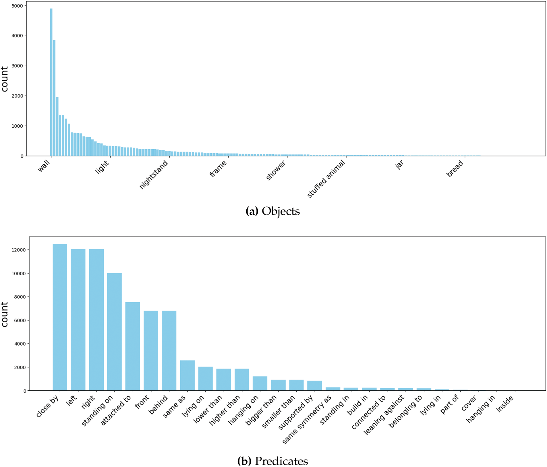
Figure 3: Class-wise distribution of objects and predicates in 3DSSG, (a) is the distribution of data counts by class for objects, and (b) is the distribution of data counts by class for predicates

4.2 Metrics

In conformance with the experimental setup detailed in 3DSSG [15], the 3D scenes were consistently placed within the same coordinate system during both the training and testing phases. To assess the accuracy of object and predicate predictions, we employed the top-k accuracy (A@k) metric [24]. To evaluate the triplets, we calculate triplet scores by multiplying the scores of the subject, predicate, and object, and subsequently determined A@k as the evaluation criterion. A triplet is deemed accurate only if all its components–subject, predicate, and object–are correctly identified. To provide a balanced assessment of performance with a long-tailed distribution, we computed the average top-k accuracy, named the average top-k accuracy (mA@k), over all predicate and object classes [24].

4.3 Implementation Details

Our network had a batch size of eight, and used the AdamW optimizer [41,42]. We trained for 100 epochs on an NVIDIA A100 GPU. This took approximately 48 hours. The learning rate was 0.0001 and we followed a cosine annealing learning rate strategy. The Pytorch platform was used [43] with the parameters set as follows: λobj=λproto=0.1, λrel=1. We referenced the object (λobj) and predicate (λrel) learning weights used in our previous work (VL-SAT) [24]. The newly added prototype loss ℒProto is used to improve object performance, which plays a similar role to ℒobjoracle in vl-sat [24]. Therefore, we set λproto to equal the hyperparameter weights of ℒobjoracle. The point cloud was sampled using 128 points, and all embedding vectors inside the model including the prototype dimension, were set to 512 dimensions.

4.4 Comparison with State-of-the-Art Methods

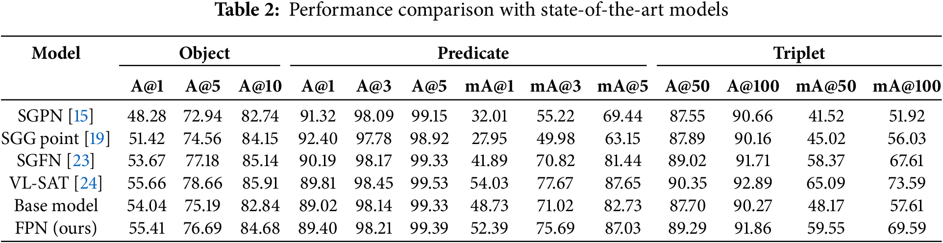
Table 2 shows the performance of our model compared to state-of-the-art models. The VL-SAT model is multimodal, and the rest are single models, such as ours. The base model is similarly to the SGFN [23] and non-VL-SAT [24] models. The FPN was trained by applying a prototypical loss in to the base model. Overall, the base model appeared to perform similarly to the SGFN model. Object performs somewhat worse than the SGFN model, and predicate performs somewhat worse, but slightly better regarding average top-k accuracy. This suggests that the base model performs slightly worse than SGFN but is more robust to long-tailed distributions. Triplet performed poorly overall compared to SGFN. Comparing the base model to our FPN, we observed a substantial performance increase across objects, predicates, and triplets. Object exhibited performance improvement of A@1 1.37, A@5 1.5, and A@10 1.84. Predicate performed similarly for A@K, but shows a substantial improvement in average top-k accuracy with mA@1 3.66, mA@3 4.67, and mA@5 4.3. The triplet also shows an overall performance improvement, especially in the average top-k accuracy, with mA@50 of 11.38 and mA@100 of 11.98. This indicates that embedding the node features resulting from graph reasoning into the prototype space improves the overall performance of the model. The improvement in average top-k accuracy across the different parts also shows that our FPN can train well on data with long-tailed distributions. This trend is similar for VL-SAT multimodal model, showing that embedding in a prototype space allows a single model to extract as much information as a multimodal models.

4.5 Comparison by Data Distribution for Different Backbone Models

In this section, the experimental reports are divided into three categories based on the number of objects and predicates per class: Head, Body, and Tail, respectively. In addition, we applied the proposed fusion-loss method to the SGFN [23] and VL-SAT [24] models. For experimental fairness, only 3D models were used for the VL-SAT multimodal model.

Table 3 shows that for objects, applying fusion loss improves the overall performance. Except for the mA@1 metric of the body part in SGFN and the mA@5 metric of the head part in VL-SAT, the performance improved. In particular, the model with FPN in the tail part shows a substantial performance improvement, with mA@1 of 0.46, mA@5 of +4.78, and mA@10 of +2.16 for SGFN, and mA@1 of +1.86, mA@5 of +6.79, and mA@10 of +16.89 for VL-SAT. These substantial performance improvements in the tail part demonstrate that FPN can capture the features of sparsely labeled objects in a general scene graph prediction model.

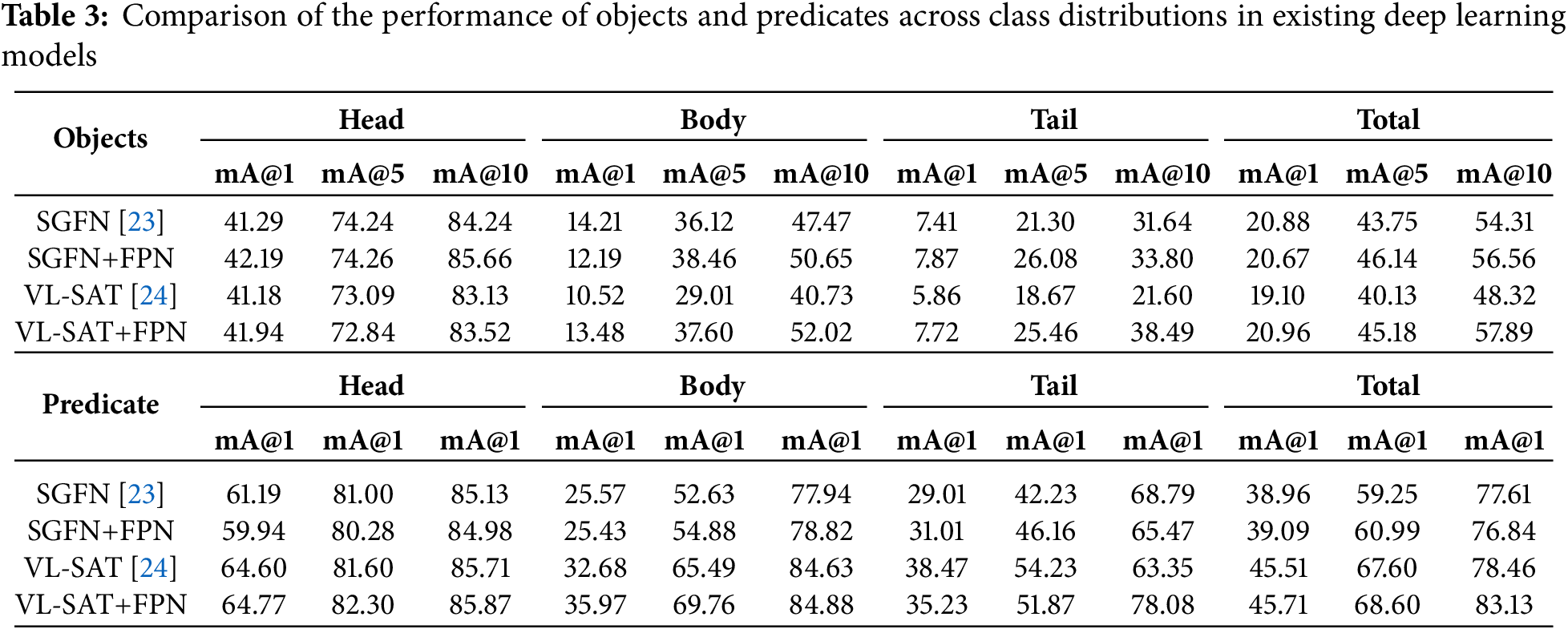
Objects show consistent performance gains per backbone, while predicates show average performance gains but no consistency in performance gains per backbone. This suggests that the model does not mitigate backbone-specific architectural disparities, which is probably due to the model primarily focusing on object prototypes.

4.6 Qualitative Results

In this section, we compared the base model, ground truth, and our proposed FPN. The input point cloud, the ground-truth graph, the base model’s prediction graph, and the proposed FPN’s prediction graph are depicted in Fig. 4. Each label denotes an object, and each line represents its relationship with other objects. The arrowheads signify the directions of the linkages. A red arrow indicates an incorrect prediction of no relationship. The base model incorrectly predicted three nodes, while FPN incorrectly predicted four nodes. In some cases, our method misclassified sparse classes like “toilet” as many classes like “chair”. In general, FCN performed better on the edges. The base model predicted numerous “no relationship” overall, and our methods occasionally incorrectly predicted some relationships.

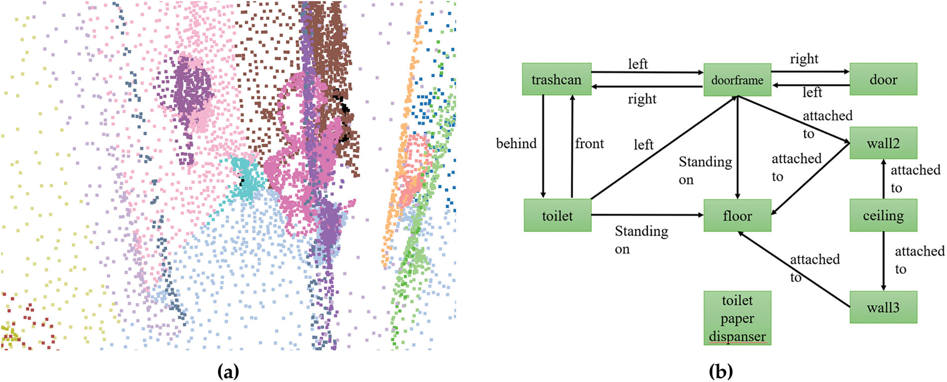
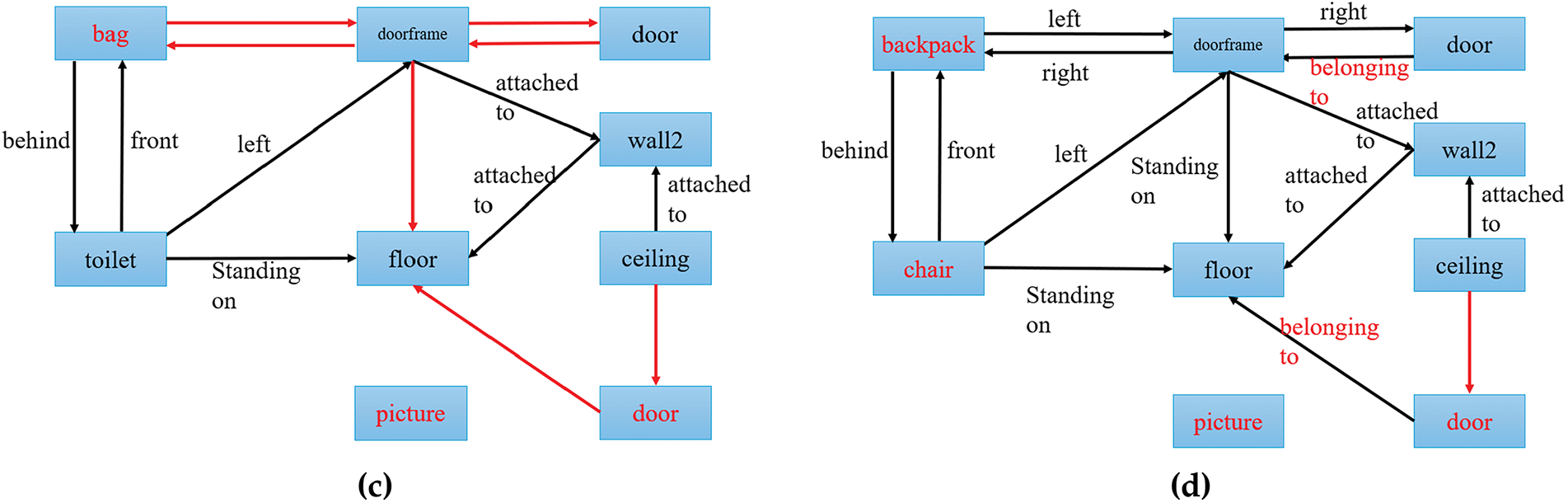
Figure 4: Qualitative evaluation of the proposed method compared to the base model and ground truth; (a) is the input point cloud, (b) is the ground truth graph, (c) is the base model prediction graph, and (d) is the FPN’s prediction graph

5  Discussion

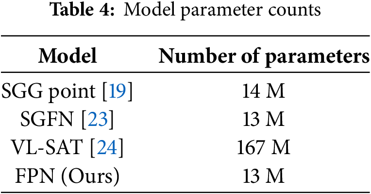
In general, multimodal models that combine images and language perform well overall by effectively utilizing semantic information from images and contextual information from language. However, these models are disadvantaged by requiring additional computing resources to utilize multiple modalities. Table 4 shows the number of parameters per model. Multi-modal models such as VL-SAT [24] use a CLIP encoder [30] for image and language alignment, which requires more computing resources than a single model. Although our model has a slight difference in performance compared to VL-SAT [24], we can achieve similar performance with fewer computing resources.

6  Conclusion

We present a FPN that leverages the potential space of an existing scene graph prediction neural network as a prototype. By embedding this space and utilizing a prototype-based mapping strategy, the FPN effectively captures underrepresented classes, addressing the challenges posed by long-tailed distributions. Evaluating it on the 3DSSG dataset shows clear performance gains as a single model and demonstrates robustness to long-tailed distributions of objects and triplets. This provides a more balanced representation of complex 3D environments. However, the model focuses on capturing sparse classes of objects and does not improve performance for predicates. In future work, we will further explore sparse class capture for both objects and predicates, aiming for a more comprehensive understanding and representation of the relationships in complex scenes.

Acknowledgement: None.

Funding Statement: This work was supported by the Glocal University 30 Project Fund of Gyeongsang National University in 2025.

Author Contributions: Study conception and design: Jiho Bae, Suwon Lee; data collection: Bogyu Choi, Sumin Yeon; analysis and interpretation of results: Jiho Bae, Suwon Lee; draft manuscript preparation: Jiho Bae, Bogyu Choi, Sumin Yeon; revision of the manuscript: Jiho Bae, Suwon Lee. All authors reviewed the results and approved the final version of the manuscript.

Availability of Data and Materials: The data and materials used in this study are currently part of an ongoing project and cannot be publicly released at this time. Access to the data may be considered upon reasonable request after the completion of the project.

Ethics Approval: Not applicable.

Conflicts of Interest: The authors declare no conflicts of interest to report regarding the present study.

References

1. Zhu G, Zhang L, Jiang Y, Dang Y, Hou H, Shen P, et al. Scene graph generation: a comprehensive survey. arXiv:2201.00443. 2022. [Google Scholar]

2. Xu D, Zhu Y, Choy CB, Fei-Fei L. Scene graph generation by iterative message passing. In: Proceedings of the 2017 IEEE Conference on Computer Vision and Pattern Recognition; 2017 Jul 21–26; Honolulu, HI, USA. p. 5410–9. [Google Scholar]

3. Chang X, Ren P, Xu P, Li Z, Chen X, Hauptmann A. A comprehensive survey of scene graphs: generation and application. IEEE Transact Pattern Anal Mach Intell. 2021;45(1):1–26. doi:10.1109/tpami.2021.3137605. [Google Scholar] [PubMed] [CrossRef]

4. Li Y, Ouyang W, Zhou B, Wang K, Wang X. Scene graph generation from objects, phrases and region captions. In: Proceedings of the 2017 IEEE International Conference on Computer Vision; 2017 Oct 22–29; Venice, Italy. p. 1261–70. [Google Scholar]

5. Anthes C, García-Hernández RJ, Wiedemann M, Kranzlmüller D. State of the art of virtual reality technology. In: 2016 IEEE Aerospace Conference; 2016 Mar 5–12; Big Sky, MT, USA. p. 1–19. [Google Scholar]

6. Burdea GC, Coiffet P. Virtual reality technology. Hoboken, NJ, USA: John Wiley & Sons; 2003. [Google Scholar]

7. Guttentag DA. Virtual reality: applications and implications for tourism. Tourism Manag. 2010;31(5):637–51. doi:10.1016/j.tourman.2009.07.003. [Google Scholar] [CrossRef]

8. Javaid M, Haleem A. Virtual reality applications toward medical field. Clin Epidemiol Global Health. 2020;8(2):600–5. doi:10.1016/j.cegh.2019.12.010. [Google Scholar] [CrossRef]

9. Azuma RT. A survey of augmented reality. Presence: Teleoperat Virtual Environ. 1997;6(4):355–85. [Google Scholar]

10. Billinghurst M. Augmented reality in education. New Horiz Learn. 2002;12(5):1–5. [Google Scholar]

11. Nee AY, Ong S, Chryssolouris G, Mourtzis D. Augmented reality applications in design and manufacturing. CIRP Annals. 2012;61(2):657–79. doi:10.1016/j.cirp.2012.05.010. [Google Scholar] [CrossRef]

12. Shalal N, Low T, McCarthy C, Hancock N. A review of autonomous navigation systems in agricultural environments. In: SEAg 2013: Innovative Agricultural Technologies for a Sustainable Future; 2013 Sep 22–25; Barton, ACT, Australia. [Google Scholar]

13. Golroudbari AA, Sabour MH. Recent advancements in deep learning applications and methods for autonomous navigation: a comprehensive review. arXiv:2302.11089. 2023. [Google Scholar]

14. Alkendi Y, Seneviratne L, Zweiri Y. State of the art in vision-based localization techniques for autonomous navigation systems. IEEE Access. 2021;9:76847–74. doi:10.1109/access.2021.3082778. [Google Scholar] [CrossRef]

15. Wald J, Dhamo H, Navab N, Tombari F. Learning 3D semantic scene graphs from 3D indoor reconstructions. In: Proceedings of the 2020 IEEE/CVF Conference on Computer Vision and Pattern Recognition; 2020 Jun 13–19; Seattle, WA, USA. p. 3961–70. [Google Scholar]

16. Wald J, Avetisyan A, Navab N, Tombari F, Nießner M. RIO: 3D object instance re-localization in changing indoor environments. In: Proceedings of the 2019 IEEE/CVF International Conference on Computer Vision; 2019 Oct 27–Nov 2; Seoul, Republic of Korea. p. 7658–67. [Google Scholar]

17. Qi CR, Su H, Mo K, Guibas LJ. PointNet: deep learning on point sets for 3D classification and segmentation. In: Proceedings of the 2017 IEEE Conference on Computer Vision and Pattern Recognition; 2017 Jul 21–26; Honolulu, HI, USA. p. 652–60. [Google Scholar]

18. Phan AV, Le Nguyen M, Nguyen YLH, Bui LT. DGCNN: a convolutional neural network over large-scale labeled graphs. Neural Networks. 2018;108(4):533–43. doi:10.1016/j.neunet.2018.09.001. [Google Scholar] [PubMed] [CrossRef]

19. Zhang C, Yu J, Song Y, Cai W. Exploiting edge-oriented reasoning for 3D point-based scene graph analysis. In: Proceedings of the 2021 IEEE/CVF Conference on Computer Vision and Pattern Recognition; 2021 Jun 20–25; Nashville, TN, USA. p. 9705–15. [Google Scholar]

20. Zhao H, Jiang L, Jia J, Torr PH, Koltun V. Point transformer. In: Proceedings of the 2021 IEEE/CVF International Conference on Computer Vision; 2021 Oct 11–17; Montreal, BC, Canada. p. 16259–68. [Google Scholar]

21. Huang K, Yang J, Wang J, He S, Wang Z, He H, et al. Granular3D: delving into multi-granularity 3D scene graph prediction. Pattern Recognit. 2024;153(2):110562. doi:10.1016/j.patcog.2024.110562. [Google Scholar] [CrossRef]

22. Zhang S, Hao A, Qin H. Knowledge-inspired 3D scene graph prediction in point cloud. Adv Neural Inform Process Syst. 2021;34:18620–32. [Google Scholar]

23. Wu SC, Wald J, Tateno K, Navab N, Tombari F. Scenegraphfusion: incremental 3D scene graph prediction from rgb-d sequences. In: Proceedings of the 2021 IEEE/CVF Conference on Computer Vision and Pattern Recognition; 2021 Jun 20–25; Nashville, TN, USA. p. 7515–25. [Google Scholar]

24. Wang Z, Cheng B, Zhao L, Xu D, Tang Y, Sheng L. VL-SAT: visual-linguistic semantics assisted training for 3D semantic scene graph prediction in point cloud. In: Proceedings of the 2023 IEEE/CVF Conference on Computer Vision and Pattern Recognition; 2023 Jun 17–24; Vancouver, BC, Canada. p. 21560–9. [Google Scholar]

25. Zhang S, Tong H, Xu J, Maciejewski R. Graph convolutional networks: a comprehensive review. Computat Social Netw. 2019;6(1):1–23. [Google Scholar]

26. Bahdanau D, Cho K, Bengio Y. Neural machine translation by jointly learning to align and translate. arXiv:1409.0473. 2014. [Google Scholar]

27. Koch S, Vaskevicius N, Colosi M, Hermosilla P, Ropinski T. Open3DSG: open-vocabulary 3D scene graphs from point clouds with queryable objects and open-set relationships. arXiv:2402.12259. 2024. [Google Scholar]

28. Lv C, Qi M, Li X, Yang Z, Ma H. SGFormer: semantic graph transformer for point cloud-based 3D scene graph generation. In: Proceedings of the 2024 AAAI Conference on Artificial Intelligence; 2024 Feb 26–27; Vancouver, BC, Canada. p. 4035–43. [Google Scholar]

29. Koch S, Hermosilla P, Vaskevicius N, Colosi M, Ropinski T. Lang3DSG: language-based contrastive pre-training for 3D Scene Graph prediction. arXiv:2310.16494. 2023. [Google Scholar]

30. Radford A, Kim JW, Hallacy C, Ramesh A, Goh G, Agarwal S, et al. Learning transferable visual models from natural language supervision. In: 38th International Conference on Machine Learning; 2021 Jul 18–24; Online. p. 8748–63. [Google Scholar]

31. Feng M, Hou H, Zhang L, Wu Z, Guo Y, Mian A. 3D spatial multimodal knowledge accumulation for scene graph prediction in point cloud. In: Proceedings of the 2023 IEEE/CVF Conference on Computer Vision and Pattern Recognition; 2023 Jun 17–24; Vancouver, BC, Canada. p. 9182–91. [Google Scholar]

32. Koch S, Hermosilla P, Vaskevicius N, Colosi M, Ropinski T. SGRec3D: self-supervised 3D scene graph learning via object-level scene reconstruction. In: Proceedings of the 2024 IEEE/CVF Winter Conference on Applications of Computer Vision; 2024 Jan 3–8; Waikoloa, HI, USA. p. 3404–14. [Google Scholar]

33. Vinyals O, Blundell C, Lillicrap T, Wierstra D. Matching networks for one shot learning. Adv Neural Inf Process Syst. 2016;29:3637–45. [Google Scholar]

34. Snell J, Swersky K, Zemel R. Prototypical networks for few-shot learning. Adv Neural Inform Process Syst. 2017;30:4080–90. [Google Scholar]

35. Finn C, Abbeel P, Levine S. Model-agnostic meta-learning for fast adaptation of deep networks. In: 2017 International Conference on Machine Learning; 2017 Aug 6–11; Sydney, NSW, Australia. p. 1126–35. [Google Scholar]

36. Sung F, Yang Y, Zhang L, Xiang T, Torr PH, Hospedales TM. Learning to compare: relation network for few-shot learning. In: Proceedings of the IEEE Conference on Computer Vision and Pattern Recognition; 2018 Jun 18–23; Salt Lake City, UT, USA. p. 1199–208. [Google Scholar]

37. Ye HJ, Hu H, Zhan DC, Sha F. Few-shot learning via embedding adaptation with set-to-set functions. In: Proceedings of the IEEE/CVF Conference on Computer Vision and Pattern Recognition; 2020 Jun 13–19; Seattle, WA, USA. p. 8808–17. [Google Scholar]

38. Lee K, Maji S, Ravichandran A, Soatto S. Meta-learning with differentiable convex optimization. In: Proceedings of the 2019 IEEE/CVF Conference on Computer Vision and Pattern Recognition; 2019 Jun 15–20; Long Beach, CA, USA. p. 10657–65. [Google Scholar]

39. Zhou Y, Liu B, Liu Y, Jiao J. Filter bank networks for few-shot class-incremental learning. Comput Model Eng Sci. 2023;137(1):647–68. doi:10.32604/cmes.2023.026745. [Google Scholar] [CrossRef]

40. Vaswani A, Shazeer N, Parmar N, Uszkoreit J, Jones L, Gomez AN, et al. Attention is all you need. Adv Neural Inf Process Syst. 2017;30:6000–10. [Google Scholar]

41. Kingma DP, Ba J. Adam: a method for stochastic optimization. arXiv:1412.6980. 2014. [Google Scholar]

42. Loshchilov I, Hutter F. Fixing weight decay regularization in adam. arXiv:1711.05101. 2017. [Google Scholar]

43. Loshchilov I, Hutter F. SGDR: stochastic gradient descent with warm restarts. arXiv:1608.03983. 2016. [Google Scholar]