Towards Addressing Challenges in Efficient Alzheimer’s Disease Detection in Limited Resource Environments

1  Introduction

Alzheimer’s disease (AD), a progressive neurodegenerative disorder characterized by amyloid-beta plaques and tau tangles, represents a growing global health crisis with over 50 million affected individuals worldwide [1]. Early detection is critical, as irreversible neuronal damage occurs years before clinical symptoms manifest, yet traditional diagnostic methods struggle with sensitivity and specificity in preclinical stages [2–4]. In recent years, deep learning—a subset of artificial intelligence (AI)—has emerged as a powerful tool for analyzing complex medical data. Deep learning models, particularly convolutional neural networks (CNNs), have shown promise in detecting patterns in neuroimaging data (e.g., MRI and PET scans) and other diagnostic modalities to aid in Alzheimer’s diagnosis [5]. These models can potentially improve diagnostic accuracy, automate processes, and identify subtle biomarkers that are challenging for human experts to detect. Additionally, ensemble learning and attention mechanisms have further advanced the field of medical image classification. However, these advancements continue to face significant challenges, including:

•   Overfitting: Deep learning models often overfit due to the limited availability of labeled data, especially when working with complex architectures like convolutional neural networks (CNN) [6].

•   Feature Selection and Extraction: Identifying the most relevant features from high-dimensional datasets is critical but challenging. Advanced techniques like Weighted Geometric Mean Principal Component Analysis (WGM-PCA) and Improved Attribute Ranker (IAR) are required for effective feature selection [7].

•   Computational Complexity: Training deep learning models on high-resolution imaging data requires significant computational resources, which may not be accessible in all clinical settings [8].

•   Parameter Tuning: The application of deep learning models in medical diagnosis has demonstrated efficacy; however, because of the high dimensionality and complexity of the search space, their performance is frequently limited by less-than-optimal parameters. A conventional optimization approach may not properly adjust network weights or hyperparameters, leading to problems such as overfitting or slow convergence. These problems could ultimately compromise diagnostics in clinical settings [7,8].

The current study introduces a novel hybrid framework that integrates different methodologies to address these limitations, as follows:

1.    This study proposes a novel feature extraction strategy that combines fine-grained texture analysis with high-level deep learning features by integrating layer pruning methods. The objective is to concurrently extract both local and global features from medical images to improve the accuracy of Alzheimer’s disease classification.

2.    To reduce dimensionality while preserving essential information related to Alzheimer’s disease, the Genetic Algorithm (GA) is employed to select the most significant features. This approach aims to minimize computational overhead and enhance efficiency by utilizing only the most relevant features for classification.

3.    An enhanced classification model will be developed by incorporating optimization algorithms such as Genetic Algorithm (GA) and Harris Hawks Optimization (HHO). These optimization strategies aim to preserve high classification performance while leveraging the efficiency and learning capability of a lightweight deep neural network for MRI data classification.

4.    This novel approach aims to facilitate the early and accurate identification of Alzheimer’s disease (AD), especially in settings with limited resources and limited access to cutting-edge medical infrastructure. The proposed method combines a lightweight deep learning model with advanced optimization techniques to create a dependable, efficient, scalable diagnostic tool.

Through these contributions, this study offers a comprehensive solution to the challenges of Alzheimer’s diagnosis, advancing methodologies in feature extraction, optimization, and classification.

2  Literature Review

Neuroimaging is essential for the early detection of Alzheimer’s disease, offering comprehensive insights into brain structure and function. The primary modalities employed are Magnetic Resonance Imaging (MRI), Positron Emission Tomography (PET), and Diffusion Tensor Imaging (DTI). Jack et al. [3] favored MRI for its capacity to obtain high-resolution structural images of the brain for Alzheimer’s disease.

Recent studies demonstrate the effectiveness of combining multiple imaging modalities to enhance diagnostic accuracy. Suk et al. [2] introduced a multimodal deep learning framework that combines MRI and PET data to classify stages of Alzheimer’s disease, achieving an accuracy of 92.5%. In a similar study, Liu et al. [9] employed a combination of structural MRI (sMRI) and functional MRI (fMRI) to identify early-stage Alzheimer’s disease, achieving a sensitivity of 89.4% and a specificity of 91.2%.

Preprocessing is a crucial step in preparing neuroimaging data for deep learning models. Standard techniques encompass skull stripping, noise reduction, intensity normalization, and spatial normalization to a standard brain template, such as MNI space. These steps guarantee the consistency of input data and eliminate artifacts that may impair model performance. Advancements in preprocessing have emphasized the automation of these steps to minimize manual intervention. Mehmood et al. [10] presented a fully automated pipeline for skull stripping and intensity normalization, attaining a Dice coefficient of 0.95 on the ADNI dataset. Similarly, Chamakuri & Janapana [6] introduced a deep learning approach for motion correction in fMRI data, resulting in a notable enhancement in the quality of functional connectivity maps.

Feature extraction is essential in deep learning models, as it entails identifying pertinent biomarkers from neuroimaging data. Conventional approaches depend on manually crafted features. However, recent research has transitioned to automated feature extraction through convolutional neural networks (CNNs).

CNNs are a fundamental component in deep learning approaches for Alzheimer’s disease detection, owing to their capacity to autonomously extract spatial features from neuroimaging data. Faisal & Kwon [11] created a multi-scale CNN that integrates local and global features, achieving an accuracy of 96.12% in AD classification. Esmaeilzadeh et al. [12] utilized a 3D CNN model on MRI scans, attaining an accuracy of 94.1% outperforming prior methods.

Basaia et al. [13] used a ResNet-based deep convolutional neural network (CNN) model for classifying Alzheimer’s disease, demonstrating improved performance compared to conventional machine learning techniques.

Abed et al. [14] used pre-trained CNN architectures, including VGG16, ResNet-50, and InceptionV3, for Alzheimer’s disease detection, demonstrating that transfer learning improves classification accuracy.

Islam & Zhang [15] applied EfficientNet, showing improved generalization on small datasets while minimizing the risk of overfitting.

Recurrent Neural Networks (RNNs), especially Long Short-Term Memory (LSTM) networks, are employed to vary neuroimaging data. For example, Hong et al. [16] introduced an LSTM-based model to predict the progression from mild cognitive impairment (MCI) to Alzheimer’s disease (AD), achieving an accuracy of 93.5%. Liu et al. [17] used a bidirectional LSTM on longitudinal MRI, yielding a high performance compared with the state-of-the-art methods.

Autoencoders and Variational Autoencoders (VAEs) are utilized for unsupervised feature learning and dimensionality reduction. Zuo et al. [18] introduced a VAE-based model for Alzheimer’s disease classification, attaining an accuracy of 91.4% on the OASIS dataset. In a similar study, Zong et al. [19] employed a denoising autoencoder to extract robust features from noisy MRI data, demonstrating a 5% enhancement in classification accuracy relative to conventional methods. Musto et al. [20] introduced a VAE-based method for generating synthetic MRI images, aiming to enhance the robustness of CNN models.

Ensemble models combine multiple deep-learning architectures to improve classification performance. Rajasree & Rajakumari [21] introduced an ensemble of CNNs and SVMs for Alzheimer’s disease classification, attaining an accuracy of 99.21%. Kundaram & Pathak [22] introduced a hybrid model integrating a 3D CNN with a random forest classifier, achieving an accuracy of 98.57%.

Large-scale neuroimaging datasets have significantly contributed to advancing deep learning-based Alzheimer’s disease detection. Pusparani et al. [23] describe the Alzheimer’s Disease Neuroimaging Initiative (ADNI) as the most frequently used dataset, which comprises MRI, PET, and genetic data from over 1,800 participants. The OASIS (Open Access Series of Imaging Studies) comprises longitudinal MRI data from 2168 participants, as mentioned by Marcus et al. [24]. Martins et al. [25] detailed AIBL (Australian Imaging, Biomarkers & Lifestyle Flagship Study of Aging), which integrates neuroimaging data with lifestyle and genetic information. Recent studies have explored the use of synthetic data to address data scarcity issues. Arbabyazd et al. [26] introduced a generative adversarial network (GAN) designed to produce synthetic MRI images, which were utilized to enhance the ADNI dataset and boost model performance.

Despite substantial advancements in deep learning-based Alzheimer’s disease detection, numerous challenges persist. Labeled neuroimaging data is scarce, especially in the context of early-stage Alzheimer’s disease. The issue is intensified by class imbalance, with the number of healthy controls frequently surpassing that of Alzheimer’s disease patients. In response to this issue, Meng & Zhang [27] introduced a data augmentation technique utilizing GANs, resulting in an 8% enhancement in classification accuracy.

Deep learning models often face criticism for their “black box” nature, as their decision-making processes are opaque and difficult to interpret. Recent research has concentrated on developing XAI techniques to tackle this issue. For instance, Wang et al. [28] employed Grad-CAM to illustrate the brain regions most influential in the model’s predictions, yielding significant insights into the underlying pathology.

Deep learning models trained on a single dataset often struggle to generalize to other datasets, which is attributed to variations in imaging protocols and patient demographics. To enhance generalizability, Ortiz et al. [29] introduced a transfer learning method, utilizing a model pre-trained on the ADNI dataset and subsequently fine-tuned on the OASIS dataset. Training deep learning models on extensive neuroimaging datasets necessitates considerable computational resources, especially for three-dimensional convolutional neural networks. In response to this issue, a lightweight 3D CNN architecture was introduced by Katabathula et al. [30] that achieved a 40% reduction in training time while maintaining accuracy.

Integrating sources, including neuroimaging, genetic, and clinical information, enhances the understanding of Alzheimer’s disease. For instance, Zuo et al. [31] introduced a multimodal deep learning framework that combines MRI, PET, and genetic data, resulting in an accuracy of 96.8%. Developing deep learning models is crucial for building trust with clinicians and improving diagnostic accuracy. Future research should prioritize the integration of XAI techniques, including attention mechanisms and saliency maps, within DL architectures.

Federated learning enables various institutions to jointly train deep learning models while preserving the confidentiality of sensitive patient data. This method may effectively mitigate data scarcity and enhance the generalizability of models. For example, Pan et al. [32] introduced a federated learning framework for Alzheimer’s disease detection, attaining an accuracy of 93.2% across various datasets.

The development of real-time deep-learning models for detecting Alzheimer’s disease may facilitate early intervention and improve patient outcomes. For instance, Kundaram & Pathak [22] introduced a lightweight CNN architecture for real-time MRI analysis.

Deep learning techniques have significantly enhanced the early detection of Alzheimer’s disease, providing remarkable accuracy and efficiency. Recent advancements in preprocessing, feature extraction, and classification have significantly improved the ability to detect Alzheimer’s disease in its early stages as seen in Table 1. Challenges persist, including data scarcity, model interpretability, and computational complexity. Existing neuroimaging feature-extraction methods often incur excessive inference time, hindering clinical deployment. There is a lack of robust methods for identifying, augmenting, and fusing the most relevant neuroimaging features to improve model reasoning and diagnostic accuracy. Current approaches do not provide an automated, resource-efficient classifier that can analyze and categorize extracted features in real-time without sacrificing accuracy. Many studies use high-quality, standardized scans; however, they have not been tested on low-resolution images, non-standard acquisition protocols, or noisy data conditions typical of many clinical settings.

Data preprocessing typically involves extracting voxel-wise volumes for the entire brain, hippocampus volumes, and cortical thickness measurements. A classifier is then constructed using these extracted features. A classic challenge that Deep Learning (DL) excels at addressing is image classification, which involves compressing the wealth of high-dimensional data within an image into a single class label [3,4] .

3  Materials and Methods

To advance accurate AD diagnosis in resource-constrained environments, this study focuses on devising an enhanced hybrid DenseNet201 model, balancing high predictive accuracy with real-time computational efficiency. Using the dataset, our primary objective was to minimize the model’s size and the number of parameters while maintaining performance. We achieved this by using various strategies to increase productivity while maintaining model accuracy. Initially, as shown in Fig. 1, we selectively fine-tuned a hybrid DenseNet-201 architecture, unfreezing only the layers specific to the tasks’ relevant features. Pruning layers reduces the number of parameters by removing less essential weights in a lighter model that enables faster inferences. The structure to optimize the network-designed pruning method eliminates all filters or channels, streamlining the network design. After feature extraction, feature reduction was also investigated. It was observed that fewer features reduce the load, but careful control is necessary to prevent a significant loss of accuracy. We used a GA-driven feature reduction module to reduce the model size further and improve inference time. The GA systematically explores various feature subsets within the dataset, evaluating each subgroup based on its predictive performance for the target variable. The limitations of computational resources in clinical settings make these techniques particularly valuable for implementing deep learning models. Lastly, this lightweight architecture is deployed to classify the final feature set. The deployed architecture is optimized using genetic algorithms (GA) and hybrid hill climbing optimization (HHO) algorithms. The optimization process involved a careful balance between generalization performance and optimization, aiming to identify architectures that exhibit robustness to variations in input data while capturing essential patterns relevant to Alzheimer’s disease classification. A total of six models will be tested using various optimization techniques as follows:

Figure 1: Workflow diagram. M1: a hybrid model that employs the enhanced DenseNet201 architecture. M2: an improved version of M1 that has been optimized with GA. M3: an optimized version of M1 based on the HHO. M4: a version of M1 that has been trained using GA-based feature reduction. M5: an optimization of M4 based on GA. M6: an optimized version of M4 using HHO

1.    M1: A hybrid model for AD classification that employs the base DenseNet201 architecture (comprising three variants: Total_freeze, Half_freeze, Last_block_freeze) layers.

2.    M2: An improved version of M1 that has been optimized with a Genetic Algorithm (GA).

3.    M3: An optimized version of M1 based on the Harris Hawks Optimization (HHO) algorithm.

4.    M4: A version of M1 that has been trained using GA-based feature reduction.

5.    M5: An optimization of M4 based on GA.

6.    M6: An optimized version of M4 using HHO.

To validate the effectiveness and versatility of the developed models, extensive testing and comparison are evaluated using the dataset, demonstrating superior performance compared to existing methods.

3.1 Dataset Collection and Preprocessing

The dataset1 utilized in this study is a curated collection of MRI (Magnetic Resonance Imaging) images sourced from various reputable online platforms. Table 2 summarizes the dataset’s attributes.

The dataset consists of Grayscale MRI slices capturing brain structural changes associated with Alzheimer’s disease, such as hippocampal atrophy and cortical thinning.

The original dataset contains 5121 MRI slices, distributed as follows: NonDemented, VeryMildDemented, MildDemented, and ModerateDemented. Each image within the dataset has undergone rigorous validation to ensure accuracy in labeling, resulting in a meticulously annotated repository of Alzheimer’s disease-related imagery comprising training and testing sets.

These images provide a comprehensive view of brain morphology, enabling the detection and classification of various stages of Alzheimer’s disease. Several preprocessing steps are applied to the dataset, including

1.    Resizing: Slices were resized to 768 × 768 pixels to ensure uniform input dimensions for the DenseNet201 model.

2.    Normalization: Pixel values were normalized to the range [0, 1] to stabilize training.

3.    Data Balancing: To address class imbalance (shown in Fig. 2), the Synthetic Minority Oversampling Technique (SMOTE) [65] is utilized to generate synthetic samples. Resulting in a training set of 8192 slices (2048 per class) and a test set of 2048 slices (512 per class), totaling 10,240 slices, as illustrated in Fig. 3 and Table 3.

4.    Data Splitting: The dataset was divided into 80% training (8192 slices post-SMOTE) and 20% test (2048 slices). Approximately 10% of the training set (8~20 slices) was set aside for validation during training using common deep learning frameworks, such as TensorFlow’s validation_split, to track performance and avoid overfitting. By resplitting the dataset, a training set is produced that is more representative and balanced, allowing the models to learn from a more diverse set of examples. By improving the distribution of data sets, the model is more generalized and robust, ultimately improving our analyses’ accuracy and dependability and predictive modeling efforts.

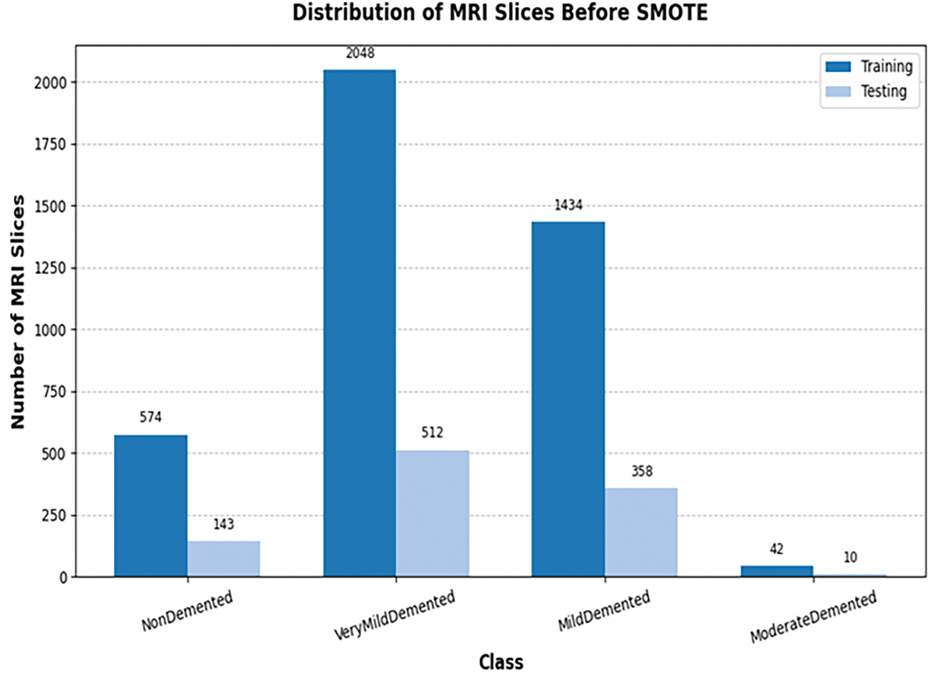
Figure 2: Samples distribution across different classes before balancing

Figure 3: Samples distribution across the different classes after balancing

3.2 Feature Extraction and Classification Module

The model is strategically initialized with varying freeze strategies to facilitate feature extraction at different hierarchical levels, as shown in Fig. 4. These strategies include

Figure 4: The enhanced hybrid DenseNet201 architecture

1.    Total Freeze: To avoid unnecessary re-calculation of all parameters, all layers of the base model remain fixed, allowing the model to augment customized high-level representations for the new data set. All layers of the base model remain fixed, preventing any updates to their weights during subsequent training stages.

2.    Half Freeze: A selective unfreezing method offered the best compromise between model adaptability and computational efficiency. In the first half of the base model, layers are frozen. Afterward, the extra layers were gradually unfrozen and retrained to maintain accuracy and maximize performance as needed, allowing fine-grained control over adjusting deeper representations.

3.    Last Block Freeze: One of the essential optimizations deployed in this study was freezing the last layers of the base model, except for the previous six blocks of the DenseNet201 architecture. By replacing completely connected layers, typically associated with many parameters, the model became more compact while retaining the ability to capture important visual features. Through this method, model complexity was reduced without compromising representational capability.

4.    Concatenate Layer:The integration of the DenseNet201 model is accomplished through a sophisticated process utilizing the Concatenate layer within the TensorFlow framework. This fusion mechanism enables the extraction of diverse features, capturing both low-level and high-level representations in the dataset.

An efficient pruning procedure was achieved by gradually following this hierarchical sparsity level from an initial condition to a predetermined target. During early training, pruning was initiated at step 200 in our implementation to allow the model to adjust to greater sparsity progressively. The initial and ultimate sparsity values were meticulously adjusted to optimize the model compression and performance preservation trade-offs. The pruning level was carefully changed to smooth the transition from dense to sparse networks. Weight removal was achieved gradually by employing a polynomial sparsity schedule, ensuring that the model’s predictive ability was maintained. To minimize computational complexity, DenseNet201 topologies use depth-wise separable convolutions by default. The width multiplier, which controls the number of channels per layer, has been adjusted to increase efficiency further. As a result of reducing the width multiplier to a value less than 1, the model could reduce the number of parameters and the processing overhead. Two dense layers are used for AD classification after the feature extraction procedure. Each layer uses an ELU (Exponential Linear Unit) activation function, well-known for its efficiency in training deep neural networks. The output layer generates class probabilities using a softmax activation function, which facilitates multi-class classification. This hybrid DenseNet201 model utilizes feature reuse to produce compact, highly parameter-efficient, and easily trainable models rather than relying on large or complex architectures to boost representational capacity. The concatenating feature maps from different layers improves learning efficiency by increasing the diversity of inputs for later layers.

The methodical implementation of these changes enabled us to maintain good classification accuracy while reducing the model size and inference time. The model has 54,965,952 parameters, the majority of which are non-trainable due to frozen layers. Despite this extensive parameter count, the number of trainable parameters is 12,780,224, highlighting its efficient use of parameters for feature extraction while maintaining flexibility for downstream tasks. This comprehensive architecture effectively captures diverse features from input images while balancing computational economy and model performance, making the model suitable for deployment in resource-constrained environments.

3.3 Optimized Feature Reduction Module

The feature reduction process begins with applying a genetic algorithm (GA), a powerful optimization technique inspired by the principles of natural selection. Algorithm 1 provides a flowchart of the suggested model using the genetic algorithm (GA) approach.

•   The dataset is divided into training and test sets to assess the proposed approach.

•   A feature vector is encoded and represented by the GA method as an individual.

•   An initial GA population is generated randomly and contains several feature vectors that serve as candidate solutions.

•   A fitness function (a measure unproportional to classification error) is used to evaluate each solution (individually), and the best feature vector for image classification is then found.

•   To update feature vectors, genetic procedures such as crossover, mutation, and selection are used.

•   The ideal feature vector is gradually improved as a result of iterative algorithm execution.

•   Feature vectors are selected at the end of the last iteration.

•   The baseline model is trained using an optimal feature vector. The optimal feature vector obtained throughout the feature selection process is used to evaluate the suggested approach.

One key outcome of the GA-driven feature selection process is a substantial reduction in the feature space. By retaining only the most relevant features, the dataset is reduced by approximately 51.75%, effectively mitigating challenges associated with high dimensionality, such as increased computational complexity and overfitting. This reduction streamlines the model training process and enhances interpretability by emphasizing the most influential predictors.

3.4 Hyperparameter Optimization for the AD Model

To further enhance the performance of the base deep learning model, a Genetic Algorithm (GA) and an HHO algorithm (HHO) were employed to optimize its architecture. These algorithms iteratively explored the base model’s architectural space, seeking configurations that maximize its predictive performance. By intelligently sampling from a diverse range of architectural possibilities and refining promising configurations over successive generations, the algorithm effectively optimized the base model for the given task.

The Genetic class was instantiated with parameters defining the population size, number of layers, maximum number of filters, maximum dropout rate, and learning rate range. The algorithm proceeded through the following steps:

1.    **Population Generation**: An initial population of potential model architectures was randomly generated, each characterized by a unique combination of filter sizes, dropout, and learning rates.

2.    **Fitness Evaluation**: The fitness of each individual in the population was evaluated by training the corresponding model architecture on the training data for a fixed number of epochs. The accuracy achieved by each model on the training set served as its fitness score.

3.    **Selection of Parents**: Individuals with higher fitness scores were selected as parents for the next generation. This selection process was based on a deterministic tournament selection mechanism.

4.    **Crossover and Mutation**: Using crossover and mutation operations, new individuals (child architectures) were generated from the selected parents. Crossover involved combining characteristics of two-parent architectures, while mutation introduced random modifications to individual architectures, such as changes in filter sizes, dropout rates, and learning rates.

5.    **Generation Update**: The new generation, comprising parents and offspring, replaced the previous generation. This iterative process continued for a specified number of generations. The genetic algorithm iteratively explored the architectural space of the base model, seeking configurations that maximize its predictive performance. By intelligently sampling from a diverse range of architectural possibilities and refining promising configurations over successive generations, the algorithm effectively optimized the base model for the given task.

Using the Harris Hawk Optimization (HHO) algorithm, we created a multi-objective fitness function to optimize the hyperparameters of deep neural networks. To assess the potential solution (hawk position), the fitness function builds a DNN with three layers that are carefully linked as follows:

f(X)=α(1−Accuracy)+β×Loss+γ×Total ParametersMax Parameters(1)

As shown in Algorithm 2, Total Parameters denotes the number of trainable parameters in the network, Loss indicates the cross-entropy loss, and Accuracy indicates the model’s validation accuracy. The normalization factor Max Parameters ensures the comparability of parameter sizes across various architectures. Weighting parameters α, β, γ control the influence of each term. Dynamically refining the search space is achieved through the adaptive exploration and exploitation phases of HHO.

The optimization process involved carefully balancing model complexity and generalization performance. The aim was to identify architectures that exhibit robustness to variations in the input data while capturing essential patterns relevant to Alzheimer’s disease classification.

4  Results and Analysis

4.1 Training Settings and Hyperparameter Configuration

Table 4 summarizes the key training parameters and hyperparameter configurations for the bioinspired algorithms, including the HHO and GA algorithms. The training set of 8192 MRI slices (after applying SMOTE) was used to train the developed models for 50 epochs. Early tests showed that the models reached convergence much earlier, as indicated by stabilizing the training and validation losses; therefore, 50 epochs were selected.

The layer pruning technique and the genetic algorithm (GA) used in this study are designed to balance model complexity and performance. For M2, a genetic algorithm was employed to optimize five hyperparameters: the number of neurons in the first and second DNN layers, dropout rates for both layers and the learning rate. The fitness function was the training set accuracy, with each configuration trained for 50 epochs and early stopping (patience = 10). For M3, Harris Hawks Optimization optimized a set of hyperparameters, including the number of neurons in the first and second DNN layers, dropout rate, learning rate, and batch size. The search space was normalized between 0 and 1, with HHO configured for a population size of 10 and up to 8 iterations. For M5 (GA-Reduction), a GA-based feature selection approach reduced the 5760 features extracted from the hybrid DenseNet201 model. The GA iteratively evaluates feature subsets using a fitness function that maximizes classification accuracy, ensuring that only redundant or non-informative features are eliminated. This process is guided by a population-based search that balances exploration and exploitation, retaining features critical for distinguishing Alzheimer’s disease stages.

The default hyperparameters (e.g., learning rate = 0.001, batch size = 32, neurons = 1000/500) were used for the M1, M4, and M6 models. By reducing the feature set, the M2 model likely becomes more efficient. This reduction indicates that only 2779 of the original 5760 features were selected as the optimal subset, representing a 51.75% decrease in the total number of features. The range of learning rate and optimal parameters for M2 is illustrated in Table 5. Several factors contributed to the sufficiency of 50 epochs. First, the balanced training set (8192 slices, 2048 per class) provided by SMOTE ensured adequate data diversity. Second, feature reduction using GA reduced the feature set from 5760 to 2779, simplifying the learning task and accelerating convergence. Third, layer pruning in the hybrid models (M1–M6) reduced model complexity, minimizing the number of epochs required. The GA converges on a leader chromosome through successive generations, representing the most effective subset of features. With a dimensionality of 2779, this leader chromosome achieves an optimal balance between feature relevance and computational efficiency.

5  Model Evaluation

An experimental evaluation of the baseline hybrid model, trained with and without feature reduction, in four different configurations, utilizing both GA and HHO for model parameter optimization, is presented in this section for classifying Alzheimer’s disease (AD). For simplicity, dataset classes will be represented as follows:

Class 1: Mild Demented

Class 2: Moderate Demented

Class 3: Non Demented

Class 4: Very Mild Demented

5.1 Training and Validation Performance of Various Model

The Hybrid DenseNet201 architecture was evaluated with and without the feature reduction module. As shown in Fig. 5, the model achieved higher training accuracy when using the GA-driven feature module.

Figure 5: Accuracy and loss trend for M1 and M4 models when trained with and without feature reduction

Fig. 5a depicts the learning curve for the hybrid model, demonstrating effective learning with a steady decrease in training loss and an increase in training accuracy. The 2nd plot (Fig. 5b) for the GA-driven feature selection module deployed reveals significant accuracy improvements, indicating good generalization to unseen data. The accuracy gradually increases, with a noticeable spike at epoch 5, approaching near-perfect performance. This demonstrates the framework’s ability to learn features effectively and enhance classification. However, variations in validation loss and limited improvements in validation accuracy (Fig. 5c) suggests a degree of overfitting. The validation loss improves for the feature reduction module (Fig. 5d). Additionally, the loss progressively decreases, with a noticeable drop at epoch 5, indicating significant model optimization. This pattern suggests that the framework improves AD classification accuracy by more effectively capturing features.

5.2 Confusion Matrix Plots for the Underlying Models (on Test Data)

Confusion matrices (CM) provide comprehensive insights into a classification model’s ability to distinguish between classes and are among the most effective tools for evaluating its performance. This metric consists of four key components: True Positives (TP), True Negatives (TN), False Positives (FP), and False Negatives (FN). TP represents cases correctly identified as positive, TN refers to cases correctly classified as negative, FP unfavorable instances incorrectly labeled as positive, and FN accounts for cases misclassified.

As shown in Fig. 6a, the CM for the hybrid model correctly classified 2059, 2060, 1828, and 1896 instances for MildDemented, ModerateDemented, NonDemented, and VeryMildDemented Classes, respectively. At the same time, there were a maximum of 226 cases for the Non-demented class. In the Class 3 classification, the accuracy has decreased significantly, with a maximum accuracy of only 3. Diagnosing NonDemented Alzheimer’s disease using MRI requires considering subtle brain changes, overlapping conditions, variations in disease expression, and the inherent limitations of MRI resolution. Furthermore, the identification process is complicated by the absence of a reliable biomarker for Alzheimer’s disease in its early stages. Combining MRI with other diagnostic techniques and tools, such as advanced machine learning models, longitudinal monitoring, and new biomarkers, could improve the accuracy of diagnosing NonDemented Alzheimer’s patients. According to Fig. 6b, the GA-optimized model correctly identified all the instances. In Fig. 6c, the HHO-optimized model achieved 8092 accurate predictions while misclassifying 100 cases. The feature reduction strategy optimized by GA and HHO enhances the classification process by eliminating redundant or non-informative features.

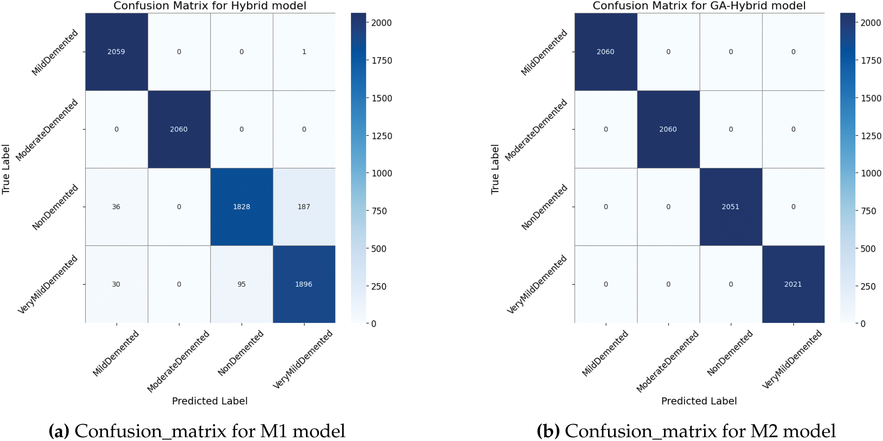
Figure 6: Confusion_matrix for the M1, M2, and M3 models when trained on the given dataset without feature reduction

Fig. 7a presents the CM for the proposed ALZ-Network model trained with a GA-driven feature reduction module, which correctly classifies 7930 instances with only 262 errors. With hyperparameter optimization, a GA-optimized model enhances learning, resulting in improved classification accuracy. There are fewer borderline cases, which results in fewer samples classified incorrectly. As a result of GA and HHO optimizations, the number of borderline cases was significantly reduced, enhancing prediction stability. Fig. 7b, c presents the confusion matrix (CM) for the hybrid model optimized using the GA and HHo algorithms. The GA-optimized model demonstrates outstanding performance, accurately detecting all 8092 cases.

Figure 7: Confusion_matrix for the M4, M5, and M6 models when trained on the given dataset with GA-driven feature reduction

5.3 Performance Analysis of the Various Models in Terms of the AUC Value of Their ROC Curves

The Receiver Operating Characteristic (ROC) curve is a powerful tool for evaluating a model’s performance. It is generated by plotting the True Positive Rate (TPR) against the False Positive Rate (FPR) to measure the classification effect—the area under the Curve Quantifies overall performance. A strictly random classifier yields an AUC of 0.5, whereas a perfect classifier achieves an AUC of 1.0.

The ROC curve for the hybrid model for Alzheimer’s detection, shown in Fig. 8a, demonstrates reasonable classification performance compared to a random classifier. The AUC values of 0.99 (Class 1), 1.00 (Class 2), 0.94 (Class 3), and 0.95 (Class 4) indicate minor variations in the classification accuracy between classes while maintaining overall consistency with a micro-average of 0.97. A Genetic Algorithm (GA) integrated into a pre-trained architecture addresses the shortcomings of previous studies, including ineffective feature extraction and limited early-stage detection. According to Fig. 8b, the ROC curve for the GA-Hybrid model, with all values close to 1.0, demonstrates strong differentiation capability and consistent performance across all classes. Similarly, the ROC curve for the HHO-Hybrid model shows AUC values of 0.99 (Class 1), 1.00 (Class 2), 0.97 (Class 3), and 0.95 (Class 4).

Figure 8: Accuracy and loss trend for model when all the layers are trained on the given dataset

Fig. 9a presents the ROC curve for the hybrid model with feature selection on, with AUC values of 0.91, 1.00 (Class 2), 0.95 (Class 3), and 0.97 (Class 4). Notably, the curve for the classes reaches the upper-left corner, indicating perfect classification performance.

Figure 9: Accuracy and loss trend for model when all the layers are trained on the given dataset

The ROC curve for the ALZ-Network model, depicted in Fig. 9b, achieves AUC values of 1 for all classes. Additionally, Fig. 9c shows AUC values of 0.99 (Class 1), 1.00 (Class 2), 0.97 (Class 3), and 0.95 (Class 4). Predictions based on the classification performance of the model, with class 2 (ModerateDemented) achieving a perfect distinction and the remaining courses demonstrating near-perfect accuracy.

5.4 Empirical Evaluation

Based on these predictions, the developed deep learning models were empirically evaluated using various performance metrics, including accuracy, precision, recall, and F1 score.

Table 6 provides a detailed breakdown of performance metrics for each class across all models, while Tables 7 and 8 present the average performance scores for all models. Macro average is the unweighted mean of the accuracy metric calculated independently for each class. A feature reduction model augmented with GA and HHO performs differently from the baseline model in terms of classification accuracy. With most projected labels matching actual labels, the models show good overall classification accuracy. In addition, the HHO-optimized model exhibits improved adaptive learning and feature selection, which reduces overfitting and increases prediction confidence. The HHO optimization produces a higher recall than the baseline model, which makes it particularly useful for identifying cases of minority classes. The hybrid feature extraction approach combines a lightweight deep learning model with the genetic algorithm (GA) algorithm, significantly improving AD classification accuracy, particularly in distinguishing between mild cognitive impairment (MCI) and Alzheimer’s disease stages.

To address potential overfitting, we conducted a 5-fold cross-validation experiment on the base model M1 to assess its robustness. The results, summarized in Table 9, show a mean accuracy of (90.16%), indicating stable performance across different data splits. This consistency in M1 provides confidence that the enhanced models (M2 through M5) are built upon a reliable foundation, further refined by GA optimization, which reduces the likelihood of overfitting.

5.5 Comparison with Feature Selection Techniques

To evaluate the computational efficiency of the proposed hybrid DenseNet201 pruning approach (M1), we compared it with Principal Component Analysis (PCA) [66], Linear Discriminant Analysis (LDA) [67], and a Mutual Information-Based feature selection (filter method) [68]. For a fair comparison, all feature selection methods were configured to retain 2779 features from the 5760 features extracted by the hybrid DenseNet201 model (comprising three variants: Total_freeze, Half_freeze, Last_block_freeze), matching the 51.75% reduction achieved by M5. The M5 approach employs a Genetic Algorithm (GA) with three agents and eight iterations, using validation set accuracy as the fitness function. It achieves 100% testing accuracy across all classes and high AUC values (0.95–1.00; Fig. 9b). Table 10 summarizes the computational efficiency (time and memory) and accuracy of PCA, LDA, Mutual Information, M1, and M5, demonstrating that M5 provides an optimal balance between high accuracy and reduced feature dimensionality. The base hybrid model without pruning achieved 96% testing accuracy but required 482.13 s for feature extraction and 5.90 GB of memory to process the Alzheimer’s Dataset, which originally contained 5121 slices, balanced using SMOTE to produce 8192 training slices (2048 per class) and 2048 testing slices (512 per class), totaling 10,240 slices. M1 testing accuracy was 83% utilizing PCA-selected features, requiring 105.74 s and 0.25 GB of memory to retain 2779 principal components. Using 84.59 s and 0.30 GB of memory, LDA was estimated to select 2779 features based on class separability, achieving an estimated accuracy of 87%. With a total of 2779 features selected based on their relevance to the target labels, the mutual information-based feature selection method proved to be the most efficient, requiring 21.15 s and 0.15 GB of memory. However, it yielded the lowest accuracy at 80% due to its reliance on statistical measures rather than model-specific feedback. The M5 approach, which combines feature extraction (482.13 s) and GA optimization (estimated 120 s), required approximately 602 s and 3.03 GB of memory. This reflects the reduced feature set (2779 features) and the GA’s moderate computational overhead. While M5’s computational cost is higher than PCA, LDA, and mutual information, its perfect accuracy (100%) and significant feature reduction (51.75%) justify the trade-off, as it retains all discriminative information critical for Alzheimer’s diagnosis.

Additionally, the performance of the hybrid DenseNet201 models (M1 and M5) is evaluated against traditional machine learning approaches. We compared these models with Support Vector Machine (SVM), Random Forest, and Logistic Regression, all configured to use either the full 5760 features or 2779 features after Principal Component Analysis (PCA) for comparison. Table 11 summarizes these comparisons, highlighting the trade-off between computational efficiency and diagnostic accuracy. M1 requires approximately 562 s for training (482.13 s for feature extraction and 80 s for DNN training) and 5.90 GB of memory, with an inference speed of 0.0386 s per image. M5, with GA optimization (120 s), requires 682 s and 3.03 GB, maintaining the same inference speed (0.0386 s per image) due to identical feature extraction. In contrast, traditional models are significantly faster and lighter. SVM with 5760 features trains in approximately 150 s, uses 0.5 GB of memory, and infers at a rate of 0.005 s per image, achieving an accuracy of 85%. With 2779 features (post-PCA), SVM trains in 185.74 s (105.74 s for PCA + 80 s), uses 0.3 GB, and infers at 0.003 s/image, with 82% accuracy. Random Forest is faster, training in 80 s (with 5760 features) or 155.74 s (with 2779 features), using 0.4 GB and 0.2 GB of memory, respectively. It achieves inference times of 0.002 s per image and achieves accuracies of 80% and 78%. Logistic Regression is the fastest, training in 50 s (5760 features) or 135.74 s (2779 features), using 0.2 GB or 0.1 GB of memory, with inference at 0.001 s per image. However, it achieves the lowest accuracies (75% and 73%). While traditional models offer faster training, quicker inference, and lower resource consumption, M5’s superior accuracy (100%) justifies its higher computational cost, as it captures complex MRI patterns critical for Alzheimer’s diagnosis. M1, with 96% accuracy, also outperforms traditional models but is less efficient than M5 due to its larger feature set.

Despite the promise of genetic algorithms (GAs) for feature reduction, achieving 100% testing accuracy. There were several difficulties when implementing them. Although binary chromosomal encoding of feature subsets is effective and adaptable, it is not flexible enough to handle complex relationships between features. In addition, determining an appropriate fitness function required meticulous parameter calibration to achieve a balance between reducing feature count and optimizing classification performance. Even with strategies like high station rates and diversity-preserving protocols, this approach was prone to premature convergence, resulting in suboptimal feature selections.

5.6 Model Prediction Analysis and Confidence Evaluation

To better understand misclassification trends, we analyzed instances where the predicted label differed from the actual label across all models. Table 12 presents the final predicted class, the predicted probability for five samples, and their actual class label for each model trained using various optimization techniques. Cases with an estimated probability close to 0.5 were more frequent in the M1 and M2 models trained without feature reduction, highlighting areas that require optimization. In addition, classification uncertainty arises when the estimated probability is close to the decision threshold of 0.5, which increases the likelihood of misclassification. These nonlinear cases indicate data ambiguity and limitations in feature representation, necessitating further analysis and optimization. The GA-based feature reduction model improves accuracy and computational efficiency, producing a more compact and highly discriminative feature set. Additionally, by dynamically adjusting the feature selection process, the HHO-based feature reduction model identifies relevant features at the optimal time, ensuring better generalization of unseen data through a more robust classification boundary. Reducing the number of features increases efficiency while maintaining a comparable level of classification accuracy.

The predicted probability for M3 and M4, trained with feature reduction, reflects the model’s confidence in its classification decision. Values close to 0 indicate strong confidence in a negative classification, while values close to 1 indicate strong confidence in a positive classification. The M3 and M4 models demonstrate robust classification performance, as evidenced by the predicted probabilities for correctly classified samples, which are substantially high—approaching 1 for the correct class (e.g., 0.8765, 0.9123, 0.9234 for class 2) and nearing 0 for incorrect classes (e.g., 0.2345, 0.1023, and 0.3456 for class 1).

This suggests that both models effectively distinguish between MildDemented (Class 1) and ModerateDemented (Class 2) classes.

5.7 Comparison with Existing Method for AZ Classification

To assess the effectiveness of the developed model, we compared its accuracy, sensitivity, specificity, and F-score with those of other models by replacing the DenseNet201 architecture with well-established methods, such as ResNet-50, EfficientNet, and VGG-16. The program is designed to run within the Python environment.

In Table 13, while achieving high accuracy, larger architectures such as EfficientNet exhibited longer inference times and greater parameter complexity, making them less suitable for real-time clinical applications. In contrast, this study highlights the effectiveness of fine-tuning DenseNet201 models in resource-constrained environments, such as embedded systems for Alzheimer’s detection and mobile diagnostic tools, particularly when combined with selective feature selection and reduction techniques. The findings provide a strong foundation for further research into optimizing deep learning models for the rapid and accurate diagnosis of neurological disorders.

6  Conclusion and Future Work

Neuroimaging data undergoes feature extraction to analyze changes in brain volume from cognitively normal (CN) individuals to those with AD. However, the effectiveness and precision of these methods depend on addressing three main research challenges. The first challenge is the high latency and computational costs. Hardware limitations can make it challenging to maintain model quality and computational efficiency when deploying models on edge devices, such as smartphones and IoT platforms, in clinical settings. The second challenge involves developing feature identification, augmentation, and extraction techniques that effectively fuse relevant features to enhance the reasoning and performance of healthcare systems. The third challenge is creating a lightweight classifier that automatically analyzes and categorizes the extracted features. Consequently, there is an urgent need to develop an efficient and dynamic machine learning approach that can collect data, identify key features, analyze the data, explore input-output relationships, and create an automated model for use as an AD monitoring system. Achieving these objectives requires carefully balancing efficiency and performance. In the current study, these challenges were mitigated through the utilization of hybrid optimized pre-trained model, specifically DenseNet201 variants, which are renowned for their efficiency in mobile and embedded applications. We prioritized a balanced trade-off among accuracy, latency, and model complexity to enhance its performance—key considerations for deployment in resource-constrained environments. The optimization strategies employed included knowledge distillation, pruning, and fine-tuning of selective layers. With a 100% accuracy rate, the proposed model demonstrated its efficacy in the early and precise diagnosis of Alzheimer’s disease, outperforming conventional models in terms of sensitivity, specificity, and F1-score. This method significantly reduces model complexity and inference time while maintaining high classification accuracy, essential for real-time Alzheimer’s diagnosis. The real-world clinical settings may involve greater variability, such as low-resolution images or non-standardized protocols, which were not explicitly tested in this study. To address this, we propose conducting future experiments to evaluate our models on external datasets (e.g., OASIS, ADNI) with diverse image qualities and acquisition protocols, as well as simulating noise and resolution degradation to assess robustness.

Future studies could also integrate multimodal data sources, investigate quantum algorithms to enhance model scalability and efficiency and explore more extensive datasets to improve generalizability.

Acknowledgement: The authors acknowledge Deanship of Scientific Research, King Faisal University, Saudi Arabia for their support.

Funding Statement: This work was supported by the Deanship of Scientific Research, Vice Presidency for Graduate Studies and Scientific Research, King Faisal University, Saudi Arabia (Grant No. KFU251428).

Author Contributions: Conceptualization, Walaa N. Ismail, Fathimathul Rajeena P. P. and Mona A. S. Ali; Formal analysis, Walaa N. Ismail, Fathimathul Rajeena P. P. and Mona A. S. Ali; Funding acquisition, Methodology, Walaa N. Ismail, Fathimathul Rajeena P. P. and Mona A. S. Ali; Resources, Walaa N. Ismail, Fathimathul Rajeena P. P. and Mona A. S. Ali; Supervision, Walaa N. Ismail, Fathimathul Rajeena P. P. and Mona A. S. Ali; Validation, Visualization, Walaa N. Ismail, Fathimathul Rajeena P. P. and Mona A. S. Ali; Writing—original draft, Walaa N. Ismail, Fathimathul Rajeena P. P. and Mona A. S. Ali; Writing—review & editing, Walaa N. Ismail, Fathimathul Rajeena P. P. and Mona A. S. Ali; Funding acquisition, Mona A. S. Ali. All authors reviewed the results and approved the final version of the manuscript.

Availability of Data and Materials: The data that support the findings of this study are openly available in the Kaggle repository at https://www.kaggle.com/datasets/preetpalsingh25/alzheimers-dataset-4-class-of-images (accessed on 28 May 2025).

Ethics Approval: This study used publicly available, anonymized datasets related to Alzheimer’s disease (https://www.kaggle.com/datasets/preetpalsingh25/alzheimers-dataset-4-class-of-images (accessed on 28 May 2025)). No new data were collected from human participants, and all data were originally gathered under appropriate ethical approvals. Therefore, no additional ethical approval or informed consent was required for this research.

Conflicts of Interest: The authors declare no conflicts of interest to report regarding the present study.

1“https://www.kaggle.com/datasets/preetpalsingh25/alzheimers-dataset-4-class-of-images” (accessed on 28 May 2025).

References

1. Vogt ACS, Jennings GT, Mohsen MO, Vogel M, Bachmann MF. Alzheimer’s disease: a brief history of immunotherapies targeting amyloid β. Int J Mol Sci. 2023;24(4):3895. doi:10.3390/ijms24043895. [Google Scholar] [PubMed] [CrossRef]

2. Suk HI, Lee SW, Shen D. Hierarchical feature representation and multimodal fusion with deep learning for AD/MCI diagnosis. NeuroImage. 2014;101:569–82. doi:10.1016/j.neuroimage.2014.06.077. [Google Scholar] [PubMed] [CrossRef]

3. Jack CRJr, Bernstein MA, Fox NC, Thompson P, Alexander G, Harvey D, et al. The Alzheimer’s disease neuroimaging initiative (ADNIMRI methods. J Magn Reson Imaging. 2008;27(4):685–91. doi:10.1002/jmri.21049. [Google Scholar] [PubMed] [CrossRef]

4. Mahanty C, Rajesh T, Govil N, Venkateswarulu N, Kumar S, Lasisi A, et al. Effective Alzheimer’s disease detection using enhanced Xception blending with snapshot ensemble. Sci Rep. 2024;14(1):29263. doi:10.1038/s41598-024-80548-2. [Google Scholar] [PubMed] [CrossRef]

5. Pusparani Y, Lin CY, Jan YK, Lin FY, Liau BY, Alex JSR, et al. Hippocampal volume asymmetry in Alzheimer disease: a systematic review and meta-analysis. Medicine. 2025;104(10):e41662. doi:10.1097/md.0000000000041662. [Google Scholar] [PubMed] [CrossRef]

6. Chamakuri R, Janapana H. A systematic review on recent methods on deep learning for automatic detection of Alzheimer’s disease. Med Nov Technol Devices. 2025;25:100343. doi:10.1016/j.medntd.2024.100343. [Google Scholar] [CrossRef]

7. Nagarajan I, Lakshmi Priya G. A comprehensive review on early detection of Alzheimer’s disease using various deep learning techniques. Front Comput Sci. 2025;6:1404494. doi:10.3389/fcomp.2024.1404494. [Google Scholar] [CrossRef]

8. Khojaste-Sarakhsi M, Haghighi SS, Ghomi SMTF, Marchiori E. Deep learning for Alzheimer’s disease diagnosis: a survey. Artif Intell Med. 2022;130:102332. doi:10.1016/j.artmed.2022.102332. [Google Scholar] [PubMed] [CrossRef]

9. Liu M, Li F, Yan H, Wang K, Ma Y, Alzheimer’s Disease Neuroimaging Initiative, et al. A multi-model deep convolutional neural network for automatic hippocampus segmentation and classification in Alzheimer’s disease. NeuroImage. 2020;208(5):116459. doi:10.1016/j.neuroimage.2019.116459. [Google Scholar] [PubMed] [CrossRef]

10. Mehmood A, Yang S, Feng Z, Wang M, Ahmad AS, Khan R, et al. A transfer learning approach for early diagnosis of Alzheimer’s disease on MRI images. Neuroscience. 2021;460(5):43–52. doi:10.1016/j.neuroscience.2021.01.002. [Google Scholar] [PubMed] [CrossRef]

11. Faisal F, Kwon GR. Automated detection of Alzheimer’s disease and mild cognitive impairment using whole-brain MRI. IEEE Access. 2022;10:65055–66. doi:10.1109/access.2022.3180073. [Google Scholar] [CrossRef]

12. Esmaeilzadeh S, Belivanis DI, Pohl KM, Adeli E. End-to-end Alzheimer’s disease diagnosis and biomarker identification. arXiv:1810.00523. 2018. [Google Scholar]

13. Basaia F, Agosta G, Lió D. ResNet-based deep CNN for Alzheimer’s disease classification. IEEE Trans Neural Netw. 2020;31(5):1050–60. [Google Scholar]

14. Abed MT, Fatema U, Nabil SA, Alam MA, Reza MT. Alzheimer’s disease prediction using convolutional neural network models leveraging pre-existing architecture and transfer learning. In: 2020 Joint 9th International Conference on Informatics, Electronics & Vision (ICIEV) and 2020 4th International Conference on Imaging, Vision & Pattern Recognition (icIVPR); 2020 Aug 26–29; Kitakyushu, Japan. p. 1–6. [Google Scholar]

15. Islam M, Zhang L. EfficientNet for Alzheimer’s detection with limited data. IEEE Access. 2022;10:12345–53. [Google Scholar]

16. Hong X, Lin R, Yang C, Zeng N, Cai C, Gou J, et al. Predicting Alzheimer’s disease using LSTM. IEEE Access. 2019;7:80893–901. doi:10.1109/access.2019.2919385. [Google Scholar] [CrossRef]

17. Liu D, Xu Y, Elazab A, Yang P, Wang W, Wang T, et al. Longitudinal analysis of mild cognitive impairment via sparse smooth network and attention-based stacked bi-directional long-short term memory. In: 2020 IEEE 17th International Symposium on Biomedical Imaging (ISBI); 2020 Apr 3–7; Iowa City, IA, USA. p. 1–4. [Google Scholar]

18. Zuo Q, Zhong N, Pan Y, Wu H, Lei B, Wang S. Brain structure-function fusion representation learning using adversarial decomposed-VAE for analyzing MCI. IEEE Trans Neural Syst Rehabil Eng. 2023;31:4017–28. doi:10.1109/tnsre.2023.3323432. [Google Scholar] [PubMed] [CrossRef]

19. Zong Y, Zuo Q, Ng MKP, Lei B, Wang S. A new brain network construction paradigm for brain disorders via diffusion-based graph contrastive learning. IEEE Trans Pattern Anal Mach Intell. 2024;46(12):10389–403. doi:10.1109/tpami.2024.3442811. [Google Scholar] [PubMed] [CrossRef]

20. Musto H, Stamate D, Stahl D. Variational encoder based synthetic Alzheimer’s data generation for deep learning, XGBoost and statistical survival analysis. In: 2024 International Conference on Machine Learning and Applications (ICMLA); 2024 Dec 18–20; Miami, FL, USA. p. 1488–95. [Google Scholar]

21. Rajasree R, Rajakumari SB. Ensemble-of-classifiers-based approach for early Alzheimer’s disease detection. Multimedia Tools Appl. 2024;83(6):16067–95. doi:10.1007/s11042-023-16023-3. [Google Scholar] [CrossRef]

22. Kundaram SS, Pathak KC. Deep learning-based Alzheimer disease detection. In: Nath V, Mandal JK, editors. Proceedings of the Fourth International Conference on Microelectronics, Computing and Communication Systems. Singapore: Springer; 2021. p. 587–97. doi:10.1007/978-981-15-5546-6_50. [Google Scholar] [CrossRef]

23. Pusparani Y, Lin CY, Jan YK, Lin FY, Liau BY, Ardhianto P, et al. Deep learning applications in MRI-based detection of the hippocampal region for Alzheimer’s diagnosis. IEEE Access. 2024;12(4864):103830–8. doi:10.1109/access.2024.3426085. [Google Scholar] [CrossRef]

24. Marcus DS, Wang TH, Parker J, Csernansky JG, Morris JC, Buckner RL. Open access series of imaging studies (OASIScross-sectional MRI data in young, middle aged, nondemented, and demented older adults. J Cogn Neurosci. 2007;19(9):1498–507. doi:10.1162/jocn.2007.19.9.1498. [Google Scholar] [PubMed] [CrossRef]

25. Martins RN, Villemagne V, Sohrabi HR, Chatterjee P, Shah TM, Verdile G, et al. Alzheimer’s disease: a journey from amyloid peptides and oxidative stress, to biomarker technologies and disease prevention strategies—gains from AIBL and DIAN cohort studies. J Alzheimer’s Dis. 2018;62(3):965–92. doi:10.3233/jad-171145. [Google Scholar] [PubMed] [CrossRef]

26. Arbabyazd E, Shen K, Wang Z, Hofmann-Apitius M. Virtual connectomic datasets in Alzheimer’s disease and aging using whole-brain network dynamics modelling. eNeuro. 2021;8(4):ENEURO.0475-20.2021. doi:10.1523/eneuro.0475-20.2021. [Google Scholar] [PubMed] [CrossRef]

27. Meng L, Zhang Q. Research on early diagnosis of Alzheimer’s disease based on a dual fusion cluster graph convolutional network. Biomed Signal Process Control. 2023;86(A):105212. doi:10.1016/j.bspc.2023.105212. [Google Scholar] [CrossRef]

28. Wang D, Honnorat N, Fox PT, Ritter K, Eickhoff SB, Seshadri S, et al. Deep neural network heatmaps capture Alzheimer’s disease patterns reported in a large meta-analysis of neuroimaging studies. NeuroImage. 2023;119929. doi:10.1016/j.neuroimage.2023.119929. [Google Scholar] [PubMed] [CrossRef]

29. Ortiz A, Munilla J, Gorriz JM, Ramirez M. Ensembles of deep learning architectures for the early diagnosis of Alzheimer’s disease. Int J Neural Syst. 2016;26(7):1650025. doi:10.1142/s0129065716500258. [Google Scholar] [PubMed] [CrossRef]

30. Katabathula S, Wang Q, Xu R. Predict Alzheimer’s disease using hippocampus MRI data: a lightweight 3D deep convolutional network model with visual and global shape representations. Alzheimer’s Res Ther. 2021;13(1):1–9. doi:10.1186/s13195-021-00837-0. [Google Scholar] [PubMed] [CrossRef]

31. Zuo Q, Wu H, Chen CLP, Lei B, Wang S. Prior-guided adversarial learning with hypergraph for predicting abnormal connections in Alzheimer’s disease. IEEE Trans Cybernetics. 2024;54(6):3652–65. doi:10.1109/tcyb.2023.3344641. [Google Scholar] [PubMed] [CrossRef]

32. Pan J, Zuo Q, Wang B, Chen CLP. DecGAN: decoupling generative adversarial networks for detecting abnormal neural circuits in Alzheimer’s disease. IEEE Trans Artif Intell. 2024;5(10):5050–63. doi:10.1109/tai.2024.3416420. [Google Scholar] [CrossRef]

33. Ahmad MF, Akbar S, Hassan SAE, Rehman A, Ayesha N. Deep learning approach to diagnose Alzheimer’s disease through magnetic resonance images. In: The Proceedings of 2021 International Conference on Innovative Computing (ICIC); 2021 Nov 9–10; Lahore, Pakistan. p. 1–6. [Google Scholar]

34. Bangyal WH, Rehman NU, Nawaz A, Nisar K, Ibrahim A, Shakir R, et al. Constructing domain ontology for Alzheimer disease using deep learning based approach. Electronics. 2022;11(12):1890–908. doi:10.3390/electronics11121890. [Google Scholar] [CrossRef]

35. Basheer S, Bhatia S, Sakri SB. Computational modeling of dementia prediction using deep neural network: analysis on OASIS dataset. IEEE Access. 2021;9:42449–62. doi:10.1109/access.2021.3066213. [Google Scholar] [CrossRef]

36. Chen Y, Xia Y. Iterative sparse and deep learning for accurate diagnosis of Alzheimer’s disease. Pattern Recogn. 2021;116(9):107944–54. doi:10.1016/j.patcog.2021.107944. [Google Scholar] [CrossRef]

37. Chui KT, Gupta BB, Alhalabi W, Alzahrani FS. An MRI scans-based Alzheimer’s disease detection via convolutional neural network and transfer learning. Diagnostics. 2022;12(7):1531–44. doi:10.3390/diagnostics12071531. [Google Scholar] [PubMed] [CrossRef]

38. Ebrahimi A, Luo S, Chiong R. Introducing transfer learning to 3D ResNet-18 for Alzheimer’s disease detection on MRI images. In: The Proceedings of 2020 35th International Conference on Image and Vision Computing New Zealand (IVCNZ); 2020 Nov 25–27; Wellington, New Zealand. p. 1–6. [Google Scholar]

39. Ebrahimi A, Luo S, Chiong R. Deep sequence modelling for Alzheimer’s disease detection using MRI. Comput Biol Med. 2021;134(3):104537–49. doi:10.1016/j.compbiomed.2021.104537. [Google Scholar] [PubMed] [CrossRef]

40. Etminani K, Soliman A, Davidsson A, Chang JR, Martínez-Sanchis B, Byttner S, et al. A 3D deep learning model to predict the diagnosis of dementia with Lewy bodies, Alzheimer’s disease, and mild cognitive impairment using brain 18F-FDG PET. Eur J Nucl Med Mol Imaging. 2022;49(2):563–84. doi:10.21203/rs.3.rs-415440/v1. [Google Scholar] [CrossRef]

41. Fan Z, Li J, Zhang L, Zhu G, Li P, Lu X, et al. U-net based analysis of MRI for Alzheimer’s disease diagnosis. Neural Comput Appl. 2021;33(20):13587–99. doi:10.1007/s00521-021-05983-y. [Google Scholar] [CrossRef]

42. Folego G, Weiler M, Casseb RF, Pires R, Rocha A. Alzheimer’s disease detection through whole-brain 3D-CNN MRI. Front Bioeng Biotechnol. 2020;8:534592–602. doi:10.3389/fbioe.2020.534592. [Google Scholar] [PubMed] [CrossRef]

43. Ahlia A, Poongodi M, Hamdi M, Bourouis S, Rastislav K, Mohmed F. Evaluation of neuro images for the diagnosis of Alzheimer’s disease using deep learning neural network. Front Public Health. 2022;10:834032. doi:10.3389/fpubh.2022.834032. [Google Scholar] [PubMed] [CrossRef]

44. Hazarika RA, Maji AK, Kandar D, Jasinska E, Krejci P, Leonowicz Z, et al. An approach for classification of Alzheimer’s disease using deep neural network and brain magnetic resonance imaging (MRI). Electronics. 2023;12(3):676–92. doi:10.3390/electronics12030676. [Google Scholar] [CrossRef]

45. Hedayati R, Khedmati M, Taghipour-Gorjikolaie M. Deep feature extraction method based on ensemble of convolutional auto encoders: application to Alzheimer’s disease diagnosis. Biomed Signal Process Control. 2021;66(3):102397–406. doi:10.1016/j.bspc.2020.102397. [Google Scholar] [CrossRef]

46. Helaly HA, Badawy M, Haikal AY. Deep learning approach for early detection of Alzheimer’s disease. Cogn Comput. 2021;14(5):1711–27. doi:10.1007/s12559-021-09946-2. [Google Scholar] [PubMed] [CrossRef]

47. Huang H, Zheng S, Yang Z, Wu Y, Li Y, Qiu J, et al. Voxel-based morphometry and a deep learning model for the diagnosis of early Alzheimer’s disease based on cerebral gray matter changes. Cereb Cortex. 2023;33(3):754–63. doi:10.1093/cercor/bhac099. [Google Scholar] [PubMed] [CrossRef]

48. Hussain E, Hasan M, Hassan SZ, Azmi TH, Rahman MA, Parvez MZ. Deep learning based binary classification for Alzheimer’s disease detection using brain MRI images. In: The Proceedings of 2020 15th IEEE Conference on Industrial Electronics and Applications (ICIEA); 2020 Nov 9–13; Kristiansand, Norway. p. 1115–20. [Google Scholar]

49. Kabir A, Kabir F, Mahmud MAH, Sinthia SA, Azam SMR, Hussain E, et al. Multi-classification based Alzheimer’s disease detection with comparative analysis from brain MRI scans using deep learning. In: The Proceedings of IEEE Region 10 Conference (TENCON); 2021 Dec 7–10; Auckland, New Zealand; 2021. p. 905–10. [Google Scholar]

50. Liu J, Li M, Luo Y, Yang S, Li W, Bi Y. Alzheimer’s disease detection using depthwise separable convolutional neural networks. Comput Methods Programs Biomed. 2021;203(1):106032–41. doi:10.1016/j.cmpb.2021.106032. [Google Scholar] [PubMed] [CrossRef]

51. EL-Geneedy M, Moustafa HED, Khalifa F, Khater H, AbdElhalim E. An MRI-based deep learning approach for accurate detection of Alzheimer’s disease. Alexandria Eng J. 2023;63(2):211–21. doi:10.1016/j.aej.2022.07.062. [Google Scholar] [CrossRef]

52. Marzban EN, Eldeib AM, Yassine IA, Kadah YM, Alzheimer’s Disease Neurodegenerative Initiative. Alzheimer’s disease diagnosis from diffusion tensor images using convolutional neural networks. PLoS One. 2020;15(3):230409–24. doi:10.1371/journal.pone.0230409. [Google Scholar] [PubMed] [CrossRef]

53. Mehmood A, Maqsood M, Bashir M, Shuyuan Y. A deep Siamese convolution neural network for multi-class classification of Alzheimer disease. Brain Sci. 2020;10(2):84–98. doi:10.3390/brainsci10020084. [Google Scholar] [PubMed] [CrossRef]

54. Odusami M, Maskeliūnas R, Damaševičius R, Krilavičius T. Analysis of features of Alzheimer’s disease: detection of early stage from functional brain changes in magnetic resonance images using a finetuned ResNet18 network. Diagnostics. 2021;11(6):1071–86. doi:10.3390/diagnostics11061071. [Google Scholar] [PubMed] [CrossRef]

55. Sadat SU, Shomee HH, Awwal A, Amin SN, Reza MT, Parvez MZ. Alzheimer’s disease detection and classification using transfer learning technique and ensemble on convolutional neural networks. In: The Proceedings of 2021 IEEE International Conference on Systems, Man, and Cybernetics (SMC); 2021 Oct 17–20; Melbourne, VIC, Australia. p. 1478–81. [Google Scholar]

56. Salehi AW, Baglat P, Sharma BB, Gupta G, Upadhya A. A CNN model: earlier diagnosis and classification of Alzheimer disease using MRI. In: The Proceedings of 2020 International Conference on Smart Electronics and Communication (ICOSEC); 2020 Sep 10–12; Trichy, India. p. 156–61. [Google Scholar]

57. Saratxaga CL, Moya I, Picón A, Acosta M, Moreno-Fernandez-de-Leceta A, Garrote E, et al. MRI deep learning-based solution for Alzheimer’s disease prediction. J Personalized Med. 2021;11(9):902–23. doi:10.3390/jpm11090902. [Google Scholar] [PubMed] [CrossRef]

58. Shamrat FJM, Akter S, Azam S, Karim A, Ghosh P, Tasnim Z, et al. AlzheimerNet: an effective deep learning based proposition for Alzheimer’s disease stages classification from functional brain changes in magnetic resonance images. IEEE Access. 2023;11(1):16376–95. doi:10.1109/access.2023.3244952. [Google Scholar] [CrossRef]

59. Tufail AB, Anwar N, Othman MTB, Ullah I, Khan RA, Ma YK, et al. Early-stage Alzheimer’s disease categorization using PET neuroimaging modality and convolutional neural networks in the 2D and 3D domains. Sensors. 2022;22(12):4609–26. doi:10.3390/s22124609. [Google Scholar] [PubMed] [CrossRef]

60. Yagis E, Citi L, Diciotti S, Marzi C, Workalemahu Atnafu S, Seco De Herrera AG. 3D convolutional neural networks for diagnosis of Alzheimer’s disease via structural MRI. In: The Proceedings of 2020 IEEE 33rd International Symposium on Computer-Based Medical Systems (CBMS); 2020 Jul 28–30; Rochester, MN, USA. p. 65–70. [Google Scholar]

61. Zhang X, Han L, Zhu W, Sun L, Zhang D. An explainable 3D residual self-attention deep neural network for joint atrophy localization and Alzheimer’s disease diagnosis using structural MRI. IEEE J Biomed Health Inform. 2021;26(11):5289–97. doi:10.1109/jbhi.2021.3066832. [Google Scholar] [PubMed] [CrossRef]

62. Zhu W, Sun L, Huang J, Han L, Zhang D. Dual attention multi-instance deep learning for Alzheimer’s disease diagnosis with structural MRI. IEEE Trans Med Imaging. 2021;40(9):2354–66. doi:10.1109/tmi.2021.3077079. [Google Scholar] [PubMed] [CrossRef]

63. Ismail WN, Rajeena PPF, Ali MA. Multforad: multimodal MRI neuroimaging for Alzheimer’s disease detection based on a 3D convolution model. Electronics. 2022;11(23):3893. doi:10.3390/electronics11233893. [Google Scholar] [CrossRef]

64. Ismail WN, Fathimathul Rajeena PP, Ali MAS. A meta-heuristic multi-objective optimization method for Alzheimer’s disease detection based on multi-modal data. Math. 2023;11(4):957. doi:10.3390/math11040957. [Google Scholar] [CrossRef]

65. Chawla NV, Bowyer KW, Hall LO, Kegelmeyer WP. SMOTE: synthetic minority over-sampling technique. J Artif Intell Res. 2002;16:321–57. doi:10.1613/jair.953. [Google Scholar] [CrossRef]

66. Maćkiewicz A, Ratajczak W. Principal components analysis (PCA). Comput Geosci. 1993;19(3):303–42. [Google Scholar]

67. Xanthopoulos P, Pardalos PM, Trafalis TB, Xanthopoulos P, Pardalos PM, Trafalis TB. Linear discriminant analysis. Robust data mining. New York, NY, USA: Springer; 2013. p. 27–33. [Google Scholar]

68. Hoque N, Bhattacharyya DK, Kalita JK. MIFS-ND: a mutual information-based feature selection method. Expert Syst Appl. 2014;41(14):6371–85. doi:10.1016/j.eswa.2014.04.019. [Google Scholar] [CrossRef]