
 Submit a Paper
 Propose a Special lssue
 Open Access
ARTICLE
Shape Sensitivity Analysis of Acoustic Scattering with Series Expansion Boundary Element Methods
1 Key Laboratory of In-Situ Property-Improving Mining of Ministry of Education, Taiyuan University of Technology, Taiyuan, 030024, China
2 Henan International Joint Laboratory of Structural Mechanics and Computational Simulation, School of Architecture and Civil Engineering, Huanghuai University, Zhumadian, 463000, China
* Corresponding Author: Haojie Lian. Email:
Computer Modeling in Engineering & Sciences 2025, 143(3), 2785-2809. https://doi.org/10.32604/cmes.2025.066001
Received 27 March 2025; Accepted 12 May 2025; Issue published 30 June 2025
 View Full Text
 Download PDF
Abstract
This study explores a sensitivity analysis method based on the boundary element method (BEM) to address the computational complexity in acoustic analysis with ground reflection problems. The advantages of BEM in acoustic simulations and its high computational cost in broadband problems are examined. To improve efficiency, a Taylor series expansion is applied to decouple frequency-dependent terms in BEM. Additionally, the Second-Order Arnoldi (SOAR) model order reduction method is integrated to reduce computational costs and enhance numerical stability. Furthermore, an isogeometric sensitivity boundary integral equation is formulated using the direct differentiation method, incorporating Cauchy principal value integrals and Hadamard finite part integrals to handle singularities. The proposed method improves the computational efficiency, and the acoustic sensitivity analysis provides theoretical support for further acoustic structure optimization.Keywords
In modern urban environments, traffic noise pollution has become a critical environmental issue, significantly impacting daily life, work efficiency, and public health [1,2]. With the rapid advancement of urbanization, traffic volumes on highways, railways, and city roads have surged, exacerbating noise pollution and diminishing residents’ quality of life [3,4]. Prolonged exposure to high noise levels has been linked to serious health risks, including hearing impairment, sleep disturbances, and cardiovascular diseases. Addressing this growing concern necessitates effective noise mitigation strategies and advanced acoustic modeling techniques [5,6].
Among the traffic noise control measures, sound barriers are widely used along highways, railways, and urban roads because of their significant noise reduction effect and convenient construction. Sound barriers mainly block the propagation path of noise and reduce the noise level in the far field area, thereby improving the acoustic environment in the noise-affected area [7]. However, the noise reduction performance of traditional sound barriers is limited by material properties, geometric shapes, and surrounding environmental factors, and it is difficult to maintain a good attenuation effect under different noise frequencies and complex scenarios. In addition, the impact of ground reflection on noise propagation cannot be ignored. The design of optimized sound barriers needs to comprehensively consider ground effects, boundary conditions, and noise propagation characteristics to improve the overall noise reduction capability.
The boundary element method (BEM) has long been recognized as a powerful tool for acoustic analysis, particularly in solving unbounded field problems. Unlike finite element methods (FEM), BEM discretizes only the boundary of the domain, drastically reducing computational effort while maintaining high fidelity in capturing wave phenomena such as diffraction, reflection, and scattering. This feature makes BEM particularly advantageous for road noise prediction and noise barrier optimization. Pioneering work by Rizzo [8] laid the foundation for BEM in elastodynamics, which later expanded into acoustics, as demonstrated by Hothersall et al. [9] in their studies on barrier shape effects and ground reflections. Subsequent advancements, including fast multipole methods (FMM), adaptive integration techniques, and hybrid collocation schemes for coupled vibro-acoustic problems, further enhanced BEM’s applicability to large-scale engineering problems [10,11].
Despite its strengths, conventional BEM faces critical challenges in broadband acoustic computations. The frequency-dependent kernel function necessitates repetitive reconstruction of system matrices across frequency bands, leading to prohibitive computational costs and memory demands for large-scale problems [12–14]. Many approaches have been proposed to address this limitation [15–19], recent innovations integrate Taylor series expansions to decouple the kernel function into frequency-dependent and frequency-independent components. By precomputing and reusing frequency-independent terms, this approach significantly reduces computational overhead while preserving accuracy, thereby extending BEM’s utility to wideband noise barrier optimization [20,21]. Notably, the modified singular boundary method (SBM) introduced by Wu et al. [22] incorporates a combined Helmholtz integral equation formulation and self-regularization technique, which improves the accuracy and efficiency of numerical solutions, especially in external acoustics.
This study integrates Taylor-expanded BEM with reduced-order computation for sensitivity analysis of noise barrier structures. By employing Taylor series expansion, the frequency-dependent kernel is decomposed into separable components, enabling efficient reuse of precomputed terms across broadband frequencies [23–26]. Furthermore, a reduced-order model is adopted to alleviate the computational burden associated with large-scale matrices [27–29]. To overcome singularities inherent in boundary integral equations, Cauchy principal value integration and Hadamard finite-part integration are systematically applied, ensuring numerical stability and accuracy. The proposed isogeometric sensitivity boundary integral equation, based on the direct differentiation method, facilitates efficient sensitivity evaluation with respect to control point coordinates. This methodology not only enhances the computational efficiency of broadband acoustic optimization but also provides a theoretical foundation for acoustic optimization calculations.
Specifically, the research content of this section includes the following aspects:
1. Acoustic modeling of ground reflection: Based on the image source method, the sound field integral equation including the ground reflection effect is established, and its influence on the acoustic response is analyzed.
2. Derivation of acoustic sensitivity formula: Based on the formula in Section 3, the direct differential method derivation considering the ground reflection term is extended to construct a new sensitivity analysis formula.
3. Broadband calculation and order reduction implementation: Taylor expansion is performed on the sensitivity formula under ground reflection conditions, and the system order reduction is completed in combination with the SOAR method to reduce the calculation scale and memory requirements [30,31].
4. Numerical verification and analysis: For typical acoustic problems, numerical simulations including ground reflection conditions are performed to verify the accuracy of the derived formula and the effectiveness of the order reduction method.
2 Acoustic State Analysis Using IGABEM
Isogeometric Boundary Element Method (IGABEM) is an advanced computational approach for acoustic state analysis, leveraging the smooth basis functions of Non-Uniform Rational B-Splines to enhance numerical accuracy and geometric representation [32]. By integrating geometric modeling with numerical simulation, IGABEM reduces discretization errors and improves solution continuity, making it particularly effective for solving Helmholtz equations in unbounded acoustic domains [33–36]. This method enables precise analysis of sound propagation, diffraction, and scattering while maintaining computational efficiency. It is widely applied in acoustic state analysis to evaluate sound field characteristics in complex engineering scenarios, such as noise control and structural acoustics.
By combining Isogeometric Analysis (IGA) [37–39] and the Boundary Element Method (BEM), IGABEM utilizes Non-Uniform Rational B-Splines (NURBS) as basis functions for both geometry representation and physical field approximation [40,41]. NURBS are widely used in Computer-Aided Design (CAD) due to their ability to accurately model complex curves and surfaces with fewer control points compared to traditional polynomial-based methods, eliminating the geometric discretization errors that often occur in traditional methods [42]. The rational form of NURBS allows exact representation of conic sections (e.g., circles, ellipses) that cannot be captured by standard polynomials, ensuring geometric fidelity in acoustic domains with curved boundaries. Such preservation is particularly critical for acoustic simulations, where boundary conditions (e.g., impedance or pressure distributions) are highly sensitive to geometric accuracy. In the constructed curve, the coordinates of any arbitrary point can be represented as follows:
in which the coordinates of the control point are denoted by
where
For boundary integral calculation in IGABEM, Gauss-Legendre quadrature is needed to handle singular and nearly singular kernels appearing in the Helmholtz integral equation.
2.2 IGABEM Formulations for Acoustic State Analysis with NURBS
This subsection provides a detailed explanation of the isogeometric boundary element formulation used to calculate the radiated and scattered acoustic fields generated by incident waves. Initially, the commonly employed Burton-Miller boundary integral equation is utilized to accurately evaluate the acoustic pressure field at all frequencies, as follows [43,44]:
in which
where
The assumed ideal conditions of the 2D full-space acoustics are often not met in actual engineering. In many application scenarios such as urban noise control, sound barrier design, and architectural acoustic analysis, the sound field is often affected by complex boundary conditions. Ground reflection, as a common boundary effect, will significantly change the distribution characteristics and sensitivity of the sound field. Therefore, ignoring ground reflection can lead to deviations in sensitivity calculations, which can affect the reliability of design and optimization.
In order to be closer to actual engineering needs, we derive the acoustic formula of a two-dimensional half-space, which refers to a scenario that introduces ground reflection conditions in acoustic analysis. Its core feature is that sound wave propagation includes not only the direct path, but also the impact of the ground reflection path on the sound field distribution. In the analysis of urban traffic noise or building noise, the modeling of two-dimensional half-space and ground reflection is equivalent. The study of this model is essentially to accurately describe the sound field distribution and sound pressure changes under complex boundary conditions. The ground reflection effect is particularly significant in the near-surface area. The sound pressure superposition effect caused by it will change the propagation law of noise, which is of great significance to the design of noise barriers and the optimization of the sound environment around buildings. In order to effectively deal with the impact of ground reflection on the sound field distribution, this chapter introduces the mirror point processing method.
The core idea of the mirror point method is to regard the ground as the symmetric boundary of the sound wave, and to construct the mirror point of the sound source below the ground, so that the ground reflection is equivalent to the mirror sound source in the whole space. The position of the mirror point is determined by the symmetry relationship of the original sound source relative to the ground, and its acoustic characteristics are consistent with the original sound source, but the corresponding correction coefficient may be introduced due to the sound absorption characteristics of the ground. This method greatly simplifies the sound field modeling under ground reflection conditions, so that it can be directly applied to the sound field superposition calculation. The fundamental solution for half-space problems, referred to as
As shown in Fig. 1, in Eq. (6),
where
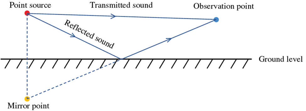
Figure 1: The propagation of sound waves emitted by the source (considering ground reflection).
In the framework of IGABEM, the geometry is constructed by discretizing the physical field using NURBS basis functions.
Since NURBS fundamental functions don’t have the Kronecker-delta characteristic,
Substituting Eqs. (1) and (9) into Eq. (7) and evaluating the equation at the discrete collocation point
in which subscript
where the matrices
where
where the
From Eq. (8), it can be inferred that a wave number k exists in the kernel function, resulting in Eq. (12) being frequency-dependent. This frequency dependence leads to high computational costs when solving broadband problems, as the coefficient matrix must be recalculated at each frequency point. To address this computational burden, a Taylor series expansion is employed in this study to decouple the kernel function into frequency-dependent and frequency-independent components, as described in the following process.
3 Acoustic Shape Sensitivity Analysis Using IGABEM
Shape sensitivity analysis is a method for evaluating the impact of geometric variations on system performance or objective functions. This approach enables engineers to understand how geometric modifications affect performance metrics, thereby facilitating design optimization and enhancing product performance [47,48]. In noise barrier design, shape sensitivity analysis is employed to evaluate the impact of geometric variations on noise reduction performance, thereby guiding the optimization process to enhance acoustic efficiency. By computing the sensitivities of acoustic wave reflection, diffraction, and absorption with respect to key geometric parameters, such as height, angle, and curvature, engineers can identify the most effective shape features for noise attenuation [49]. It not only improves the performance of noise barriers but also reduces material usage and costs, achieving both economic and environmental benefits.
By directly differentiating Eq. (7), the expression for acoustic shape sensitivity considering ground reflections can be derived:
The fundamental solution and its derivatives are governed by the coordinates of both the field and source points. As the shape undergoes continuous modifications, their values may be affected by variations in the shape design variables. Consequently, the sensitivities of the coordinates, represented by
in which
where
The sensitivity of boundary physical quantities is expressed using NURBS function interpolation as follows:
It is important to note that
By substituting Eqs. (1), (9), (23), and (24) into Eq. (14), the isogeometric discrete form of the sensitivity boundary integral equation is obtained as follows:
To determine all unknown boundary state values required for shape sensitivity analysis, solve Eq. (12) and use all values on the boundary and known boundary sensitivity values to solve Eq. (25). According to equation Eq. (14), let
4 Rapid Frequency Sweep Analysis of Sound Pressure
The kernel function contains the wave number k, which causes Eq. (11) to be frequency-dependent. This frequency dependence significantly increases the computational cost when solving broadband problems because the coefficient matrix needs to be recalculated at each frequency [51]. To address this computational burden, this chapter uses the Taylor series expansion method to decouple the kernel function into frequency-dependent and frequency-independent terms; and uses the SOAR method to construct a ROM that retains the key features of the original FOM to accelerate the solution process, thereby significantly improving computational efficiency [52–54].
4.1 Frequency Sweep Analysis for Acoustic Sensitivity
The first-order n-th Hankel function can be expressed as a Taylor series expansion at the fixed frequency expansion point
in which

Figure 2: Calculate the frequency band.
By substituting Eq. (26) and Eq. (15) into Eq. (14), the integral form for kernel function at the fixed frequency expansion point
where
where
By substituting Eq. (35) into Eq. (30), Eq. (30) can be rewritten as:
Substituting Eq. (26) and Eq. (15) into Eq. (14), the expanded expression of the kernel function sensitivity integral is as follows:
where
Substituting Eqs. (27), (28), (29), (36), (37) and (38) into Eq. (14), Eq. (14) can be restated as follows:
where
Since the incident wave term also involves the wave number k, it can also be expressed as a Taylor series expansion at a fixed frequency point
Assuming that the incident wave propagates in the positive direction along the axis
The expanded expression of the incident wave sensitivity value can be obtained by substituting Eq. (43) into Eq. (44) to obtain the expanded expression of the incident wave sensitivity value in Eq. (41):
with
in which
Substituting Eq. (45) into Eq. (41), Eq. (41) can be restated as follows:
By discretizing Eq. (47) using NURBS, we can get the following matrix form of shape sensitivity integral formula:
Since the acoustic IGABEM sensitivity system is linearized, the solution
where
In fact, the coefficient matrix
4.2 Dimension Reduction of IGABEM System for Acoustic Sensitivity Analysis
This study considers the scattering of the incident wave by the rigid structure boundary. Since the particle velocity on the structure boundary is zero,
Let m = 0 in Eq. (51) to create a set of frequency-independent orthogonal bases. Then Eq. (51) can be re-expressed as:
It is worth noting that Eq. (52) does not approximate the original acoustic shape sensitivity equation, but is only used to establish an orthogonal basis. By using the SOAR method, we can obtain the orthogonal basis
where
The projection subspace is then constructed using the subspace spanned by the series of The projection subspace is constructed using the span subspace of a series of nonzero columns of
The original state vector of the BEM system
After a series of derivations, we finally get the simplified system:
with
The
At the registration point on the structure boundary, the sound pressure sensitivity can be obtained by applying Eq. (56), and then the sound pressure sensitivity of any point in the sound domain can be calculated using Eq. (57).
Numerical simulations were performed using the Fortran90 programming language on a laptop featuring an Intel(R) Core(TM) i9-12900H CPU and 16 GB of RAM. In this section, sound barrier models of different shapes are employed to validate the effectiveness of the proposed algorithm.
5.1 Acoustic Scattering from an Infinitely Long Rigid Cylinder
This section analyzes the sensitivity of an infinitely long rigid cylinder. As shown in Fig. 3, the center of the circular model is located at (2 m, 2 m) and the radius is 1 m. An incident wave with an amplitude of 1, represented by

Figure 3: Design domain for sound scattering from an infinite cylinder with ground reflection.
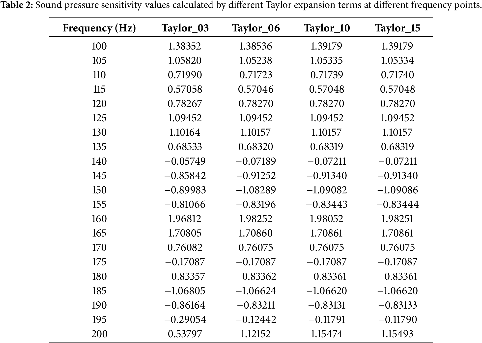
By comparing the calculation results of different numbers of Taylor expansion terms, compared with the traditional boundary element method (DBEM) that calculates each frequency point separately, the algorithm proposed in this paper uses the midpoint frequency of the interval as a fixed frequency expansion point to represent all frequency points in the interval for calculation. Therefore, the accuracy of the numerical results decreases with the increase of the distance from the fixed frequency expansion point. The frequency interval is subdivided by the adaptive band refinement technology proposed in this paper. It is finally determined that the relative error is small enough when the expansion terms are equal to or greater than 6 and the frequency band range is 50 Hz, and the fluctuation is small. After determining the relatively accurate frequency band range, we calculate the sensitivity of the acoustic model within this range.
The sensitivity of the calculation point obtained by using the algorithm taking ground reflection into account is shown in Fig. 4. It presents the results obtained by applying Taylor series expansions with 3, 6, 10, and 15 terms, respectively. The labels “Taylor

Figure 4: Sound pressure sensitivity calculated using the BEM method based on SOAR acceleration and Taylor series in two sub-intervals of different frequencies at the calculation point (0 m, 2.5 m). (a)
As shown in Fig. 4, the curves show the results of the sensitivity (
5.2 Acoustic Scattering by a Semi-Y-Shaped Noise Barrier
As shown in Fig. 5, the algorithm proposed in this chapter was used to numerically simulate the scattered sound field of the semi-Y-shaped sound barrier, and the influence of ground reflection was taken into account, with the calculation point located at (6 m, 2 m). The plane wave incident along the negative y-axis is scattered by the sound barrier. The sensitivity of the calculation point is shown in Fig. 6.

Figure 5: Design domain for sound scattering from a semi-Y-shaped with ground reflection.

Figure 6: Sound pressure sensitivity calculated using the BEM method based on SOAR acceleration and Taylor series in two sub-intervals of different frequencies at the calculation point (6 m, 2 m). (a)
As shown in Fig. 6, the figure shows the relationship between the sensitivity of
5.3 Acoustic Scattering by a Semi-Y-Shaped Concave Noise Barrier
This section studies the acoustic scattering field of a semi-Y-shaped concave sound barrier. The plane wave is incident along the negative y-axis and is scattered by the sound barrier, as shown in Fig. 7. The remaining numerical simulation parameters are the same as those given in the previous section. The algorithm proposed in this chapter is used to calculate the sensitivity of the semi-Y-shaped concave sound barrier, where the calculation point is located at (5 m, 2 m). The sensitivity of the calculation point calculated using the algorithm considering ground reflection is shown in Fig. 8.

Figure 7: Design domain for sound scattering from a semi-Y-shaped concave with ground reflection.

Figure 8: Sound pressure sensitivity calculated using the BEM method based on SOAR acceleration and Taylor series in two sub-intervals of different frequencies at the calculation point (5 m, 2 m). (a)
When using the algorithm proposed in this paper for numerical simulation, the calculation frequency interval is 25 Hz. The fixed frequency expansion point in the frequency interval
Based on the direct differential method, this paper derives the generalized acoustic sensitivity analysis formula, uses the image source method to model the acoustic effect of ground reflection, incorporates the reflection term into the framework of the boundary integral equation, constructs an acoustic analysis model suitable for two-dimensional half-space, and further derives the corresponding sensitivity formula. By performing Taylor series expansion on the sensitivity formula, not only broadband calculation is achieved, but also the size of the system matrix is effectively reduced by combining SOAR, significantly reducing memory usage and computational cost.
This method provides a theoretical framework for solving complex acoustic problems, especially large-scale broadband acoustic sensitivity analysis under complex boundary conditions, and also provides algorithmic support for subsequent optimization design. Specifically, this method provides new ideas and theoretical support for urban traffic noise control, building acoustic environment optimization, and sound barrier design. In addition, the successful application of this method in two-dimensional half-space acoustic analysis has laid the foundation for further expansion to broadband acoustic analysis of three-dimensional complex geometric shapes.
Despite these promising results, certain limitations of this study must be acknowledged. First, while the current method is designed for 2D problems, extending it to 3D geometries introduces challenges such as increased modeling complexity, greater computational demand, and more intricate treatment of singularities. Second, the boundary conditions in this study are assumed to be ideal (rigid or perfectly reflective), which may not fully represent practical scenarios involving elastic, damped, or nonlinear boundaries. Third, although the frequency decoupling strategy works effectively in most cases, its accuracy and efficiency in extremely high-frequency or highly resonant systems require further validation. Additionally, uncertainties in material properties or boundary conditions are not currently addressed, which could significantly affect real-world applications.
Addressing these issues will be a key focus of future work. The proposed method will be extended to fully coupled vibro-acoustic systems to enable more accurate simulation of interactions between structural vibrations and acoustic fields. Moreover, integration with advanced optimization algorithms—such as gradient-based or surrogate-assisted approaches—will be explored for automated acoustic design and shape optimization. Efforts will also be made to improve computational efficiency in high-frequency regimes and to extend applicability to problems involving anisotropic materials and nonlinear boundary conditions.
In terms of potential applications, the method shows great promise in various engineering domains, including acoustic optimization of high-speed train components, noise reduction in aircraft cabins, design of quiet urban zones, and the development of advanced acoustic metamaterials. Furthermore, its extension to 3D geometries opens up new possibilities for practical implementations in large-scale architectural acoustics and underwater acoustic stealth technologies.
Acknowledgement: I would like to express my sincere gratitude to Dr. Shiwei Li and Dr. Jikai Zhao for their invaluable assistance and support throughout the process of completing this thesis. Their guidance, insightful feedback, and encouragement were instrumental in shaping this work. I greatly appreciate their willingness to share their knowledge and expertise, which significantly contributed to the success of this research. Thank you both for your continuous support and dedication.
Funding Statement: This research was supported by the Shanxi Scholarship Council of China (Grant No. 2023-036) and the Natural Science Foundation of Shanxi Province (Grant No. 202303021222020).
Author Contributions: The authors confirm their contributions to this paper as follows: study conception and design: Haojie Lian, Fan Li; data collection: Hongxue Liu; analysis and interpretation of results: Fan Li, Haojie Lian, Yongsong Li; draft manuscript preparation: Hongxue Liu, Leilei Chen. All authors reviewed the results and approved the final version of the manuscript.
Availability of Data and Materials: The data that support the findings of this study are available from the corresponding author, Haojie Lian, upon reasonable request.
Ethics Approval: Not applicable.
Conflicts of Interest: The authors declare no conflicts of interest to report regarding the present study.
References
1. Jakovljevic B, Paunovic K, Belojevic G. Road-traffic noise and factors influencing noise annoyance in an urban population. Environ Int. 2009;35(3):552–6. doi:10.1016/j.envint.2008.10.001. [Google Scholar] [PubMed] [CrossRef]
2. Babisch W, Beule B, Schust M, Kersten N, Ising H. Traffic noise and risk of myocardial infarction. Epidemiol. 2005;16(1):33–40. doi:10.1097/01.ede.0000147104.84424.24. [Google Scholar] [PubMed] [CrossRef]
3. Bies DA, Hansen CH, Howard CQ, Hansen KL. Engineering noise control. Boca Raton, FL, USA: CRC Press; 2023. [Google Scholar]
4. Loncaric J, Tsynkov SV. Optimization of acoustic source strength in the problems of active noise control. SIAM J Appl Math. 2003;63(4):1141–83. doi:10.1137/s0036139902404220. [Google Scholar] [CrossRef]
5. Rahmani S, Mousavi SM, Kamali MJ. Modeling of road-traffic noise with the use of genetic algorithm. Appl Soft Comput. 2011;11(1):1008–13. doi:10.1016/j.asoc.2010.01.022. [Google Scholar] [CrossRef]
6. Ibili F, Adanu EK, Adams CA, Andam-Akorful SA, Turay SS, Ajayi SA. Traffic noise models and noise guidelines: a review. Noise Vib Worldw. 2022;53(1–2):65–79. doi:10.1177/09574565211052693. [Google Scholar] [CrossRef]
7. Qiu X. An introduction to virtual sound barriers. Boca Raton, FL, USA: CRC Press; 2019. [Google Scholar]
8. Rizzo FJ. An integral equation approach to boundary value problems of classical elastostatics. Quart Appl Math. 1967;25(1):83–95. doi:10.1090/qam/99907. [Google Scholar] [CrossRef]
9. Hothersall D, Chandler-Wilde S, Hajmirzae M. Efficiency of single noise barriers. J Sound Vib. 1991;146(2):303–22. doi:10.1016/0022-460x(91)90765-c. [Google Scholar] [CrossRef]
10. Xi Q, Fu Z, Zou M, Zhang C. An efficient hybrid collocation scheme for vibro-acoustic analysis of the underwater functionally graded structures in the shallow ocean. Comput Methods Appl Mech Eng. 2024;418:116537. doi:10.1016/j.cma.2023.116537. [Google Scholar] [CrossRef]
11. Qu Y, Zhou Z, Chen L, Lian H, Li X, Hu Z, et al. Uncertainty quantification of vibro-acoustic coupling problems for robotic manta ray models based on deep learning. Ocean Eng. 2024;299(1553):117388. doi:10.1016/j.oceaneng.2024.117388. [Google Scholar] [CrossRef]
12. Wang Z, Zhao Z, Liu Z, Huang Q. A method for multi-frequency calculation of boundary integral equation in acoustics based on series expansion. Appl Acoust. 2009;70(3):459–68. doi:10.1016/j.apacoust.2008.05.005. [Google Scholar] [CrossRef]
13. Zhang S, Yu B, Chen L. Non-iterative reconstruction of time-domain sound pressure and rapid prediction of large-scale sound field based on IG-DRBEM and POD-RBF. J Sound Vib. 2024;573:118226. doi:10.1016/j.jsv.2023.118226. [Google Scholar] [CrossRef]
14. Li S. An efficient technique for multi-frequency acoustic analysis by boundary element method. J Sound Vib. 2005;283(3–5):971–80. doi:10.1016/j.jsv.2004.05.027. [Google Scholar] [CrossRef]
15. Wu T, Li W, Seybert A. An efficient boundary element algorithm for multi-frequency acoustical analysis. J Acoust Soc Am. 1993;94(1):447–52. doi:10.1121/1.407056. [Google Scholar] [CrossRef]
16. Kirkup SM, Henwood D. Methods for speeding up the boundary element solution of acoustic radiation problems. 1992;114(3):374–80. [Google Scholar]
17. Marburg S, Schneider S. Performance of iterative solvers for acoustic problems. Part I. Solvers and effect of diagonal preconditioning. Eng Anal Bound Elem. 2003;27(7):727–50. doi:10.1016/s0955-7997(03)00025-0. [Google Scholar] [CrossRef]
18. Gao Z, Li Z, Liu Y. A time-domain boundary element method using a kernel-function library for 3D acoustic problems. Eng Anal Bound Elem. 2024;161(1553):103–12. doi:10.1016/j.enganabound.2024.01.001. [Google Scholar] [CrossRef]
19. Vanhille C, Lavie A. An efficient tool for multi-frequency analysis in acoustic scattering or radiation by boundary element method. Acta Acust United Ac. 1998;84(5):884–93. [Google Scholar]
20. Sobolev A. Wide-band sound-absorbing structures for aircraft engine ducts. Acoust Phys. 2000;46(4):466–73. doi:10.1134/1.29911. [Google Scholar] [CrossRef]
21. Zhang Q, Mao Y, Qi D, Gu Y. An improved series expansion method to accelerate the multi-frequency acoustic radiation prediction. J Comput Acoust. 2015;23(1):1450015. doi:10.1142/s0218396x14500155. [Google Scholar] [CrossRef]
22. Wu Y, Fu Z, Min J. A modified formulation of singular boundary method for exterior acoustics. Comput Model Eng Sci. 2023;135(1):377–93. doi:10.32604/cmes.2022.023205. [Google Scholar] [CrossRef]
23. Poungthong P, Giacomin A, Kolitawong C. Series expansion for normal stress differences in large-amplitude oscillatory shear flow from Oldroyd 8-constant framework. Phys Fluids. 2020;32(2):023107. [Google Scholar]
24. Cao G, Yu B, Chen L, Yao W. Isogeometric dual reciprocity BEM for solving non-Fourier transient heat transfer problems in FGMs with uncertainty analysis. Int J Heat Mass Transf. 2023;203(6):123783. doi:10.1016/j.ijheatmasstransfer.2022.123783. [Google Scholar] [CrossRef]
25. Chen L, Lian H, Xu Y, Li S, Liu Z, Atroshchenko E, et al. Generalized isogeometric boundary element method for uncertainty analysis of time-harmonic wave propagation in infinite domains. Appl Math Model. 2023;114(39–41):360–78. doi:10.1016/j.apm.2022.09.030. [Google Scholar] [CrossRef]
26. Desiderio L, Falletta S, Ferrari M, Scuderi L. CVEM-BEM coupling with decoupled orders for 2D exterior Poisson problems. J Sci Comput. 2022;92(3):96. doi:10.1007/s10915-022-01951-3. [Google Scholar] [CrossRef]
27. Chatterjee A. An introduction to the proper orthogonal decomposition. Curr Sci. 2000;78(7):808–17. [Google Scholar]
28. Shen X, Du C, Jiang S, Zhang P, Chen L. Multivariate uncertainty analysis of fracture problems through model order reduction accelerated SBFEM. Applied Mathematical Modelling. 2024;125(3–4):218–40. doi:10.1016/j.apm.2023.08.040. [Google Scholar] [CrossRef]
29. Chinesta F, Ladevèze P. Separated representations and PGD-based model reduction: fundamentals andapplications. 1st ed. Vienna, Austria: Springer; 2014. [Google Scholar]
30. Chen L, Lian H, Dong HW, Yu P, Jiang S, Bordas SP. Broadband topology optimization of three-dimensional structural-acoustic interaction with reduced order isogeometric FEM/BEM. J Comput Phys. 2024;509(9):113051. doi:10.1016/j.jcp.2024.113051. [Google Scholar] [CrossRef]
31. Bai Z. Krylov subspace techniques for reduced-order modeling of large-scale dynamical systems. Appl Numer Math. 2002;43(1–2):9–44. doi:10.1016/s0168-9274(02)00116-2. [Google Scholar] [CrossRef]
32. Gong Y, Trevelyan J, Hattori G, Dong C. Hybrid nearly singular integration for isogeometric boundary element analysis of coatings and other thin 2D structures. Comput Methods Appl Mech Eng. 2019;346(39–41):642–73. doi:10.1016/j.cma.2018.12.019. [Google Scholar] [CrossRef]
33. Zhang Y, Gong Y, Gao X. Calculation of 2D nearly singular integrals over high-order geometry elements using the sinh transformation. Eng Anal Bound Elem. 2015;60(5):144–53. doi:10.1016/j.enganabound.2014.12.006. [Google Scholar] [CrossRef]
34. Gao XW, Yang K, Wang J. An adaptive element subdivision technique for evaluation of various 2D singular boundary integrals. Eng Anal Bound Elem. 2008;32(8):692–6. doi:10.1016/j.enganabound.2007.12.004. [Google Scholar] [CrossRef]
35. Liu H, Wang F, Qiu L, Chi C. Acoustic simulation using singular boundary method based on loop subdivision surfaces: a seamless integration of CAD and CAE. Eng Anal Bound Elem. 2024;158(7):97–106. doi:10.1016/j.enganabound.2023.10.022. [Google Scholar] [CrossRef]
36. Schenck HA. Improved integral formulation for acoustic radiation problems. J Acoust Soc Am. 1968;44(1):41–58. doi:10.1121/1.1911085. [Google Scholar] [CrossRef]
37. Wang Y, Gao L, Qu J, Xia Z, Deng X. Isogeometric analysis based on geometric reconstruction models. Front Mech Eng. 2021;16(4):782–97. doi:10.1007/s11465-021-0648-0. [Google Scholar] [CrossRef]
38. Rank E, Ruess M, Kollmannsberger S, Schillinger D, Düster A. Geometric modeling, isogeometric analysis and the finite cell method. Comput Methods Appl Mech Eng. 2012;249(5–8):104–15. doi:10.1016/j.cma.2012.05.022. [Google Scholar] [CrossRef]
39. Taus MF. Isogeometric analysis for boundary integral equations[Ph.D. dissertation]. Austin, TX, USA:The University of Texas at Austin; 2015. [Google Scholar]
40. Han S, Jiang R, Gao R, Wang P. Isogeometric boundary element analysis for 2D Laplace equations. Chin J Comput Mech. 2023;40(1):105–10. [Google Scholar]
41. Piegl L, Tiller W. The NURBS book. Berlin/Heidelberg, Germany: Springer Science & Business Media; 2012. [Google Scholar]
42. Aimi A, Desiderio L, Diligenti M, Guardasoni C. Application of energetic BEM to 2D elastodynamic soft scattering problems. Commun Appl Ind Math. 2019;10(1):182–98. doi:10.1515/caim-2019-0020. [Google Scholar] [CrossRef]
43. Marburg S. The Burton and Miller method: unlocking another mystery of its coupling parameter. J Comput Acoust. 2016;24(1):1550016. doi:10.1142/s0218396x15500162. [Google Scholar] [CrossRef]
44. Burton A, Miller G. The application of integral equation methods to the numerical solution of some exterior boundary-value problems. Proc R Soc Lond A Math Phys Sci. 1971;323(1553):201–10. doi:10.1098/rspa.1971.0097. [Google Scholar] [CrossRef]
45. Lian H, Li X, Qu Y, Du J, Meng Z, Liu J, et al. Bayesian uncertainty analysis for underwater 3D reconstruction with neural radiance fields. Appl Math Model. 2025;138:115806. [Google Scholar]
46. Morse PM, Ingard KU. Theoretical acoustics. Princeton, NJ, USA: Princeton University Press; 1986. [Google Scholar]
47. Zhao W, Zheng C, Chen H. Acoustic topology optimization of porous material distribution based on an adjoint variable FMBEM sensitivity analysis. Eng Anal Bound Elem. 2019;99(1–2):60–75. doi:10.1016/j.enganabound.2018.11.003. [Google Scholar] [CrossRef]
48. Chen L, Lian H, Liu C, Li Y, Natarajan S. Sensitivity analysis of transverse electric polarized electromagnetic scattering with isogeometric boundary elements accelerated by a fast multipole method. Appl Math Model. 2025;141(47):115956. doi:10.1016/j.apm.2025.115956. [Google Scholar] [CrossRef]
49. Chen L, Huo R, Lian H, Yu B, Zhang M, Natarajan S, et al. Uncertainty quantification of 3D acoustic shape sensitivities with generalized nth-order perturbation boundary element methods. Comput Methods Appl Mech Eng. 2025;433(4):117464. doi:10.1016/j.cma.2024.117464. [Google Scholar] [CrossRef]
50. Komkov V, Choi KK, Haug EJ. Design sensitivity analysis of structural systems. Cambridge, MA, USA: Academic Press; 1986. [Google Scholar]
51. Daveau C, Aubakirov A, Oueslati S, Carre C. Boundary element method with high order impedance boundary condition for Maxwell’s equations. Appl Math Model. 2023;118(1):53–70. doi:10.1016/j.apm.2022.12.039. [Google Scholar] [CrossRef]
52. Bai ZJ, Su YF. Second-order Krylov subspace and Arnoldi procedure. J Shanghai Univ (English Edition). 2004;8(4):378–90. doi:10.1007/s11741-004-0048-9. [Google Scholar] [CrossRef]
53. Bai Z, Su Y. SOAR: a second-order Arnoldi method for the solution of the quadratic eigenvalue problem. SIAM J Matrix Anal Appl. 2005;26(3):640–59. doi:10.1137/s0895479803438523. [Google Scholar] [CrossRef]
54. Yang C. Solving large-scale eigenvalue problems in SciDAC applications. J Phys Conf Ser. 2005;16:425–35. doi:10.1088/1742-6596/16/1/058. [Google Scholar] [CrossRef]
55. Zhou H, Liu Y, Wang J. Optimizing orthogonal-octahedron finite-difference scheme for 3D acoustic wave modeling by combination of Taylor-series expansion and Remez exchange method. Explor Geophys. 2021;52(3):335–55. doi:10.1080/08123985.2020.1826890. [Google Scholar] [CrossRef]
56. Li R, Liu Y, Ye W. A fast direct boundary element method for 3D acoustic problems based on hierarchical matrices. Eng Anal Bound Elem. 2023;147:171–80. doi:10.1016/j.enganabound.2022.11.035. [Google Scholar] [CrossRef]
57. Li Y, Zhong S, Du J, Jiang X, Atroshchenko E, Chen L. Second-order Arnoldi accelerated boundary element method for two-dimensional broadband acoustic shape sensitivity analysis. Phys Fluids. 2024;36(8):086621. [Google Scholar]
58. Bai Z, Su Y. Dimension reduction of large-scale second-order dynamical systems via a second-order Arnoldi method. SIAM J Sci Comput. 2005;26(5):1692–709. doi:10.1137/040605552. [Google Scholar] [CrossRef]
59. Giacomin AJ, Saengow C, Guay M, Kolitawong C. Padé approximants for large-amplitude oscillatory shear flow. Rheolo Acta. 2015;54(8):679–93. doi:10.1007/s00397-015-0856-9. [Google Scholar] [CrossRef]
60. Junger MC, Feit D. Sound, structures, and their interaction. Vol. 225. Cambridge, MA: MIT Press; 1986. [Google Scholar]
Cite This Article
 Copyright © 2025 The Author(s). Published by Tech Science Press.
This work is licensed under a Creative Commons Attribution 4.0 International License , which permits unrestricted use, distribution, and reproduction in any medium, provided the original work is properly cited.
 Downloads
 Citation Tools