Effects of Normalised SSIM Loss on Super-Resolution Tasks

1  Introduction

In this research, we investigate the effect of incorporating a normalised Structural Similarity Index Measure (SSIM) as a component of the composite loss function used in the training of deep learning-based Super-Resolution (SR) models. The proposed approach is applied to two model architectures: a conventional Super-Resolution convolutional neural network (CNN) and an Invertible Rescaling Neural Network (IRN). Both models are trained on three commonly used benchmark datasets. We evaluate three training configurations—excluding SSIM, including SSIM in its non-normalised form, and including SSIM in its normalised form—to examine the influence of normalisation on the reconstruction quality. The results are evaluated using Peak Signal-to-Noise Ratio (PSNR), SSIM and LPIPS metrics, allowing for a comparative analysis of the reconstruction performance across all configurations.

Super-Resolution (SR) is a very demanding but fundamental artificial intelligence algorithm that is used in many practical computer vision algorithms, e.g., noise removal [1], increasing resolution on smartphones [2], person identification [3], upscaling images from laboratory measurements from micrometres to millimetres [4] and many others. In recent years, researchers have proposed various methods for solving the SR task, which is often based on deep learning, in contrast to the initially used bicubic interpolation [5], e.g., Super-Resolution generative adversarial network (SRGAN) for the task of semantic segmentation of geographic data [6], digital elevation model (DEM) for the task of flood mapping [7], full resolution class activation maps (F-CAM) based on a parametric decoder in the form of a U-net as an alternative to the previously used interpolation in this task [8], convolutional neural network (CNN) based on short-term caching for ultra-high definition (UHD) in real-time [9] and others.

The latest research Refs. [10–12] includes the principle of invertibility in the training of these models, where the image in the original size is mapped to a 4× (or even more, but with significantly worse results) reduced image using a downscale neural network, from which the upscale neural network tries to obtain an image as similar as possible to the original. The same procedure can also be used to reconstruct colours. This procedure of reducing and enlarging the image is not dissimilar in principle to an encoder and decoder or generative neural networks. Still, it uses different training and structures and layers of neural networks in all steps.

The existing results of the methods presented have shown a significant improvement in the quality of reconstructed images compared to earlier mathematical methods. However, there is still room for improvement.

It is a well-known fact that the loss function plays a key role in the overall quality of artificial intelligence algorithms, next to constructing a suitable neural network architecture, selecting a suitable optimiser and choosing an optimal learning rate value. This is no different in SR tasks. In existing published research, the choice of the loss function is given a growingly decisive role; usually, it is the Mean Square Error (MSE) comparing the original and output image, or a combination of MSE with one or more other components is used. In the research as mentioned above Refs. [10–12], the networks are trained using a combined loss function consisting of three elements—forward MSE loss, backward MSE loss and perceptual loss [13] based on feature extraction using selected layers of the pre-trained VGG19 (Visual Geometry Group) classifier.

Inverse scattering research [14] is the first research that presents LSSIM as one of the components of the composite loss function. They use MSE and the non-normalised form of Structural Similarity loss LSSIM, which is defined as:

Lfull=LMSE(y^,y)+α⋅LSSIM(y^,y)(1)

where α denotes a variable determining the representation of the component of the loss function, y^ denotes the reconstructed image, and y denotes the original image.

The component of the LSSIM(y^,y) loss function is defined as:

LSSIM(y^,y)=1−SSIM(y^,y)(2)

where the definition of similarity index SSIM, a commonly used metric designed to measure the perceptual distance between two images, is based on the original definition [15]:

SSIM(x,y)=(2μxμy+C1)(2σxy+C2)(μx2+μy2+C1)(σx2+σy2+C2)(3)

where x and y denote the images to be compared, μx,μy denote the mean brightness values of images x and y, σx,σy denote the variance (contrast) of images x and y, σxy denotes the covariance between images x and y (structure), C1 and C2 are constants preventing division by zero, where

C1=(K1L)2(4)

C2=(K2L)2(5)

where L denotes the maximum pixel value (255) and K1 and K2 are small constants (e.g., 0.01 and 0.03), and whose range of values D are:

D(SSIM)=⟨−1,1⟩(6)

whereas the value 1 indicates structural identity of the compared images, 0 indicates dissimilarity, and negative values indicate anti-correlation, although it occurs quite rarely. As shown in Fig. 1 below, the SSIM function is continuous, it accepts the input and output images, its maximisation is meaningful and differentiable, and therefore its negation can be classified as a component of the loss function [16]. The SSIM function was first defined by Wang et al. [15], as a metric evaluating the similarity between two images based on their three components—brightness, contrast and structure. Its use in the field of Super-Resolution has been popularised mainly in the framework of deep learning methods that try to maximise the visual quality of reconstructed images [15]. The importance of SSIM as a loss function was further explored in [17], where the SRGAN model was first introduced, which uses perceptual loss combined with adversarial loss. Also, work on VGG19 models [18] highlights the importance of scaling the components of the loss function in deep learning. When scaling the components of the loss functions, the same range of values should be kept for each of them, i.e., between 0 and 1.

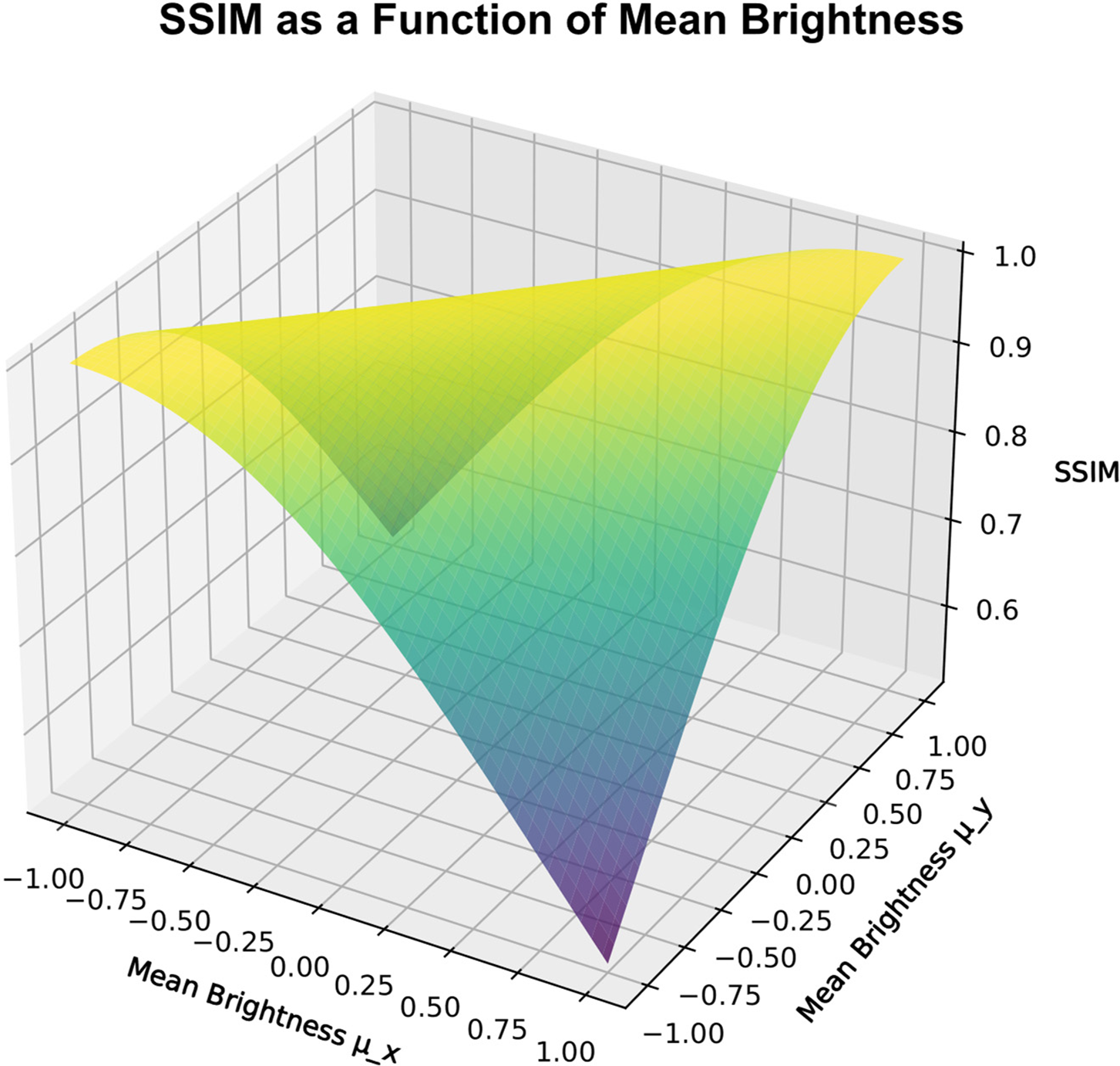
Figure 1: SSIM visualisation as a function of mean brightness

However, with a simple definition of the loss function as 1−SSIM, a situation may arise where loss values greater than 1 occur. In such a case, this component of the loss function is poorly scalable with other loss function components, which are taking values between 0 and 1. This non-normalised variant of LSSIM is also used in the latest research [19].

2  Methods

2.1 Description of the Experiment

In this research, let us assume a simultaneous training of two neural networks used for image reconstruction—downscaler and upscaler—the final purpose of which is the ability to enlarge small images with high reliability for further use in theoretical and applied research and to compare the influence of loss function components on the quality of the reconstructed image. We present an updated loss function component, the normalised similarity index loss LSSIMN and compare the image reconstruction results when it is included, not normalised and not included using standard metrics explained in Eqs. (3) and (12) to assess the impact of this component on validation subset results.

To build the downscaler and upscaler neural network architectures, we use the Keras and Tensorflow-GPU frameworks, and for training, we use the NVIDIA GeForce GTX 970 hardware with 1664 CUDA cores. As a dataset, we chose the standard DIV2K dataset [20] rescaled to 1000 × 1000 px, General100 [21], and BSDS300 [22] resized to 500 px on longer side.

We train an Invertible Rescaling Neural Network with specific blocks from VGG19 models in the perceptual loss definition as per Eq. (9). and using the same selected specific layers, we train a Super-Resolution network on all the above-mentioned benchmark datasets based on standard metrics, and we examine the influence of the loss function component LSSIMN, explained in Eq. (10).

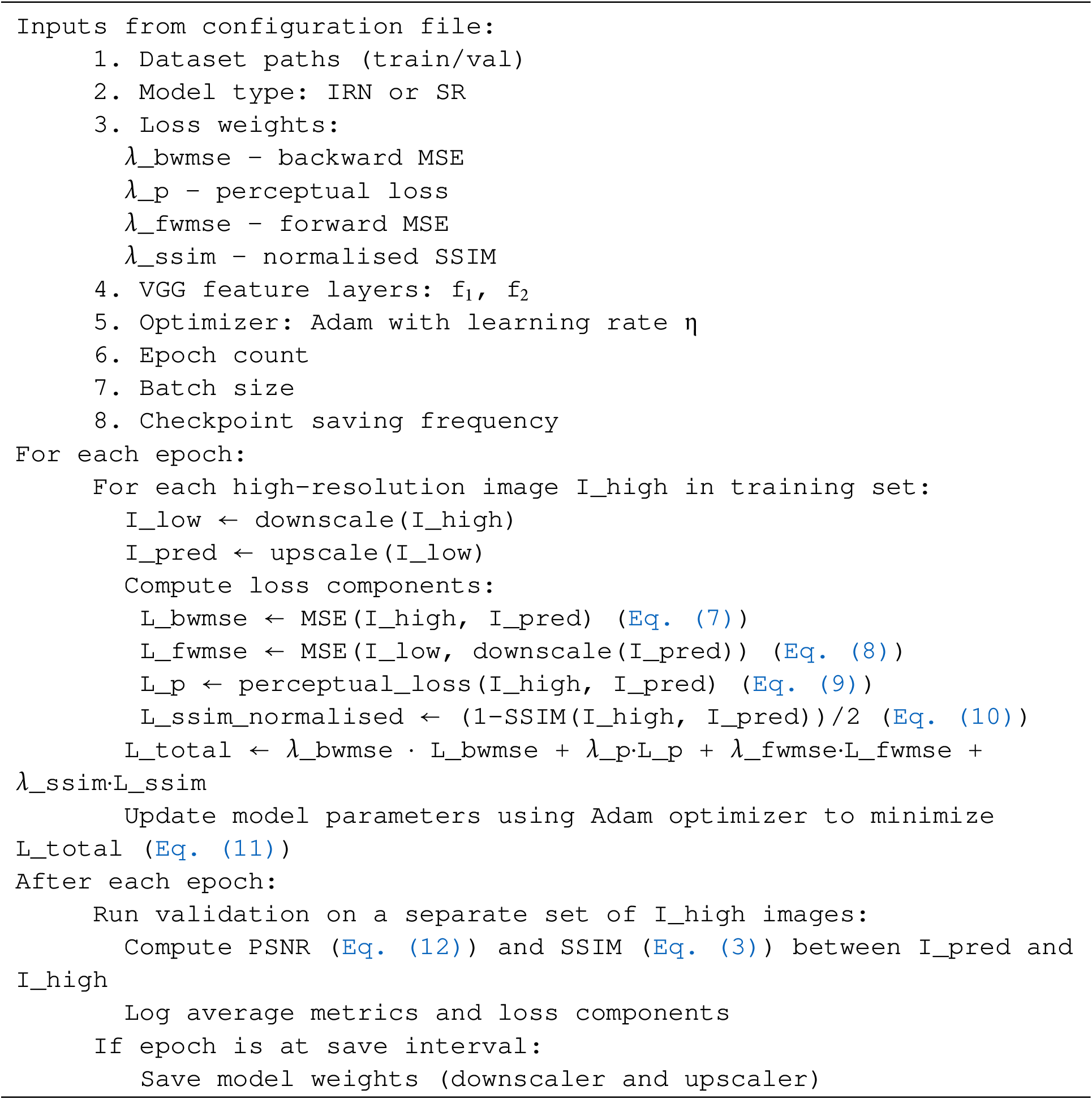
Pseudocode of the Experiment

The experimental workflow is described in the following pseudocode:

2.2 Neural Network Architectures

2.2.1 Invertible Rescaling Neural Network

Our Invertible Rescaling Neural Network uses invertible blocks in its architecture, similar to previous research Refs. [10–12]. The network consists of two subnetworks, a downscaler and an upscaler, which can be called separately during inference.

The invertible block divides the input function tensor, along the channel dimension, into two equal parts, see Fig. 2 below. The first half goes through a sequence of transformations consisting of two convolutional layers. The first convolutional layer applies a nonlinear activation function (Rectified Linear Unit—ReLU), while the second is a linear transformation. The output of this transformation is then added to the second, unchanged part of the input. This makes the transformation invertible—the original input can be reconstructed by reversing the operations.

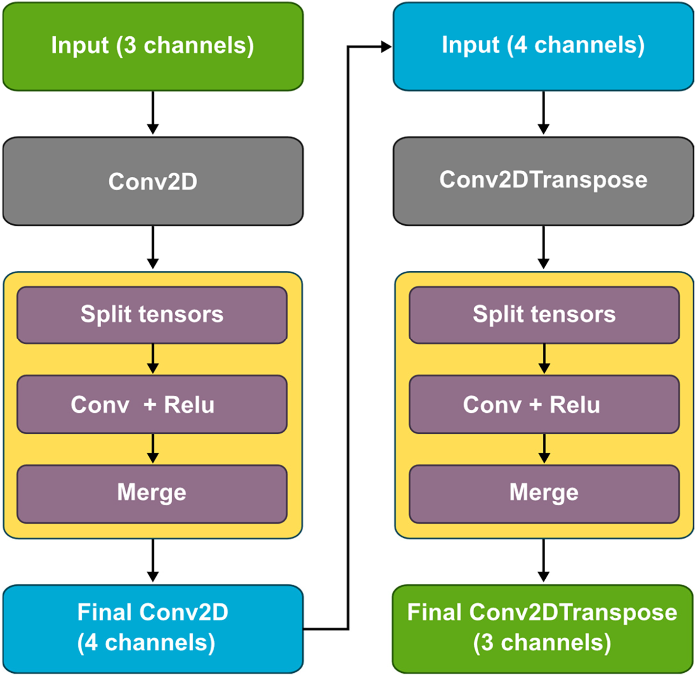
Figure 2: Invertible rescaling neural network architecture

The downscaler takes a three-channel tensor representing a normalised input image between 0 and 1 and reduces the resolution of the input image by 4×. It then applies a convolutional layer, in which the spatial resolution is reduced by a factor of two. After the convolution operation, an invertible block is applied. The number of channels in the output convolutional layer is reduced to four.

The upscaler applies reconstruction using the inverse operation of the downscaler. It takes a four-channel tensor as input, and its first layer is a transposed convolutional layer, which increases the spatial resolution by a factor of four. This is followed by an invertible block and an output layer—a transposed convolution—creating a three-channel output that matches the structure of the original image entering the downscaler.

2.2.2 Super-Resolution Network

Our Super-Resolution Network differs from the Invertible Rescaling Network primarily in that the downscaler has no trainable parameters—it is only used to reduce the image to a fractional size according to the parametric number of layers. It repeatedly applies the downscaling operation for a specified number of steps.

The upscaler transforms a 3-channel input image using a convolutional layer with 64 filters and ReLU activation, followed by a sequence of eight residual blocks, each consisting of two 3 × 3 convolutional layers, where the second layer does not apply an activation function, for explanation see Fig. 3 below. After feature extraction, the number of feature maps is increased to 256 channels, preparing the data for resampling using a pixel shuffle operation that reorganises the dimensions of the feature maps to increase spatial resolution. To improve the reconstruction, a skip join is incorporated, where the original input image is resampled using nearest neighbour interpolation, processed using a 1 × 1 convolution, and then added to the resampled feature representation. The output convolution layer adjusts the output to three channels and generates an image dimensionally corresponding to the original input to the downscaler.

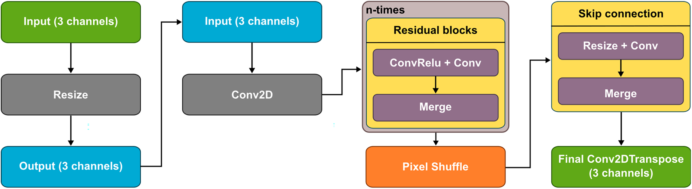
Figure 3: Super-resolution neural network architecture

2.3 Composite Loss Function

The selected loss function is composed of four components. Three of them correspond with the traditional invertible training and this work newly introduces the normalised SSIM loss LSSIMN. While there are tens of options for loss function components and hundreds of combinations, we selected LbwMSE, LfwMSE, Lperc, and LSSIMN as the components of our composite loss function because they represent commonly used, well-understood, and interpretable terms in the context of super-resolution tasks. The MSE-based components assess pixel-wise differences between original and reconstructed images, as well as between their downscaled versions. The perceptual loss, based on VGG feature activations, reflects high-level visual similarity and is widely adopted in the previously mentioned SR literature. We opted not to include additional components such as the Learned Perceptual Image Patch Similarity (LPIPS) [23] and the Charbonnier loss [24] for specific reasons. LPIPS is a learned perceptual metric whose behaviour can vary depending on the choice of pretrained network and dataset, similarly to the perceptual loss. Although it is occasionally adapted as a loss function, it is more commonly used as an evaluation metric. The Charbonnier loss, a differentiable variant of the L1 loss, is robust to outliers but would not offer specific insight into normalisation effects.

While there are many possible studies in this field, we wanted to focus our analysis on the effects of normalisation on the LSSIM on SR task and to ensure interpretability, we designed a composite loss function using standard loss components to isolate and evaluate the impact of normalisation within the composite loss structure. The selected components are:

Backward MSELbwMSE, which compares the original image with the reconstructed image, which is the output of the upscaler network:

LbwMSE=∑i=1m∑j=1n(HRij−Uij)2(7)

where HRij denotes the pixel value of the original image, Uij denotes the pixel value of the reconstructed image (upscaler output from the downscaled image), and m and n denote the dimensions of the image.

Forward MSELfwMSE, which compares the output of the downscaler of the original image with the output of the downscaler of the reconstructed image:

LfwMSE=∑i=1m∑j=1n(LRij−Dij)2(8)

where LRij denotes the pixel value of the downscaler output from the original image, Dij denotes the pixel value of the downscaler output from the reconstructed image, and m and n denote the dimensions of the image.

The perceptual loss Lperc is calculated based on the difference in features extracted using selected block in specific layers of the pretrained VGG19 model from the original and reconstructed image as:

Lperc(y,y^)=Σl∈L(1Nl)∗Σi=1Nl(Φl(y)i−Φl(y^)i)2(9)

where y denotes the original image, y^ denotes the reconstructed image, Φl(y) and Φl(y^) denote feature maps extracted from layer l of the VGG19 model, and Nl denotes the total number of elements in the feature map at layer l calculated as the product of the number of channels, the height, and the width of the feature map.

The novel normalised SSIM loss LSSIMN is calculated as:

LSSIMN=1−SSIM(y,y^)2(10)

where SSIM denotes the structural similarity value of the original image y and the reconstructed image y^ and whose range of values D(LSSIMN) is, due to the normalisation of the pixels of the images in the dataset compared to the non-normalised LSSIM [14], normalised to the interval ⟨0,1⟩ to ensure comparability with other loss function components, whose values are also in this interval when the input images are normalised. In deep learning applications, normalisation is a standard practice that helps stabilise training and prevent the dominance of any single loss component when multiple components are combined. When loss function components operate over different ranges of values, the optimiser may disproportionately prioritise larger-magnitude gradients, leading to suboptimal updates and convergence to poor local minima. By normalising the SSIM values through a linear transformation of the input image pixel range from ⟨−1,1⟩ to ⟨0,1⟩, which corresponds to min-max scaling, we make sure that this loss component contributes proportionally to the overall training and aims at a more meaningful interpretability. The overall calculation of the composite loss function Lfull is defined as:

Lfull=λb⋅LbwMSE+λf⋅LfwMSE+λp⋅Lperc+λs⋅LSSIMN(11)

2.4 Evaluation Metrics

As quantitative evaluation metrics of reconstruction quality, we chose standard metrics used for this type of task, namely SSIM according to the original definition [15] described in Eq. (3) and Peak Signal-to-Noise-Ratio PSNR according to the definition available in [25]. PSNR is a common metric for measuring image quality by comparing the original and reconstructed image using a logarithmic scale of MSE. It is calculated as follows:

PSNR[dB]=10⋅log10⁡(L2MSE)(12)

where L denotes the maximum pixel value in the image, and MSE denotes the LbwMSE loss function component.

We also incorporated Learned Perceptual Image Patch Similarity (LPIPS) [23] as an evaluation metric on the validation dataset. As noted earlier, LPIPS is not measured during training, but it serves as a validation assessment of perceptual quality. Traditional SR literature uses PSNR and SSIM. It is worth noting that LPIPS often does not correlate directly with PSNR or SSIM, which is expected and has been documented. LPIPS range of values is ⟨0,1⟩, and lower values indicate greater perceptual similarity between the reconstructed and reference images. LPIPS is defined as follows:

LPIPS(x,x′)=∑l||wl⋅(ϕl(x)−ϕl(x′)||22(13)

where ϕl(x) denotes deep feature activations from layer l of a pretrained network, wl denotes a learned scalar or vector weights (one per channel), ||⋅||22 denotes squared Euclidean norm (L2), and x and x′ denote the two images being compared.

3  Results

3.1 Invertible and Super-Resolution Networks Results

We trained two architectures, Super-Resolution and Invertible-Rescaling-Network, whose structures are described in detail in Sections 2.2.1 and 2.2.2. Training was performed by minimising the loss function defined by Eq. (11), with the weights of the individual components set as follows: λb=λf=λp=1. All coefficients λ were set to unity to ensure that each loss function component contributes equally to the training and that the same range of values is maintained across all of these three components. Setting the coefficients to unity also simplified a balanced optimisation process without introducing additional complexity that is associated with hyperparameter selection. We focused solely on the influence of the SSIM loss component on the resulting training quality, and therefore we tested the parameter λs in three variants. Thanks to this, we were able to isolate and evaluate the contribution of the SSIM component within the composite loss function, in accordance with the principles of ablation analysis.

In the first variant, we set λs=0, thus omitting the SSIM loss completely. In the second variant, we used a normalised version of the SSIM loss with the value λs=1, i.e., comparable to the other loss function components. In the third variant, we minimised the original, non-normalised SSIM loss according to Eq. (2), by setting the parameter λs=2. We applied each of these configurations to both architectures and all three benchmark datasets, making it 18 experiments in total. Table 1 summarises the dataset sizes, the number of training epochs, and the results achieved on the validation set after the first and last epochs, evaluated using the metrics given in Eqs. (3) and (12) and the losses defined by Eqs. (7) and (11). For all 18 experiments we selected the blocks ‘block4_conv4’ and ‘block5_conv4’ for feature map extraction based on experiments shown in Appendix A in calculating the perceptual loss as described in Eq. (9). In order to select these blocks, we conducted eight experiments on the DIV2K_1000 px dataset to compare the performance of different blocks in minimising perceptual loss, and the results showed that the best results were obtained by combining block3_conv2 with block4_conv4 and block4_conv4 with block5_conv4 as visible in Table A2. In order to compare the highest-level features in the original and reconstructed images, we selected the feature maps block4_conv4 and block5_conv4 for feature extraction. The detailed behaviour of the VGG19 blocks and the results of additional experiments evaluating their impact are provided in Appendix A, specifically in Tables A1 and A2.

For all experiments, training was conducted using the Adam optimiser with a fixed learning rate of 0.0005, as higher learning rates could skip over optimal solutions during convergence. No learning rate schedule or decay strategy was applied. The batch size was set to 1 due to varying image dimensions across the datasets, which made batch processing impractical without image resizing. The number of iterations per epoch corresponded to the dataset size (e.g., 100 iterations for General100, 250 for BSDS300, and 800 for DIV2K). No data augmentation techniques were used, all images were used in their original orientation and resolution. These settings, along with the associated codes and configurations, are available in the Availability of Data and Materials statement of this manuscript.

In Table 1, the columns denoted with “(start)” indicate results on the validation subset after Epoch 1, the columns denoted with “(end)” indicate results on validation subset after the epoch number specified in the column Epochs. The best results of the monitored metrics after the last epoch are marked in bold. In the table, we use colours to group related experiments together for a better interpretability. Each colour group corresponds to a specific combination of model architecture, dataset, and loss function configuration comparing different experimental conditions. The table describes how the presence or absence of the LSSIM component—whether omitted (λs = 0), used in its normalised form (λs = 1), or unnormalised (λs = 2)—influences reconstruction performance.

Across the majority of configurations, the inclusion of normalised LSSIMN (λs = 1) consistently results in improvements in SSIM scores by the final epoch, with only a minimal trade-off in PSNR or total loss. For example, in the General100 dataset with IRN, the SSIM increased from 0.7235 (λs = 0) to 0.7915 (λs = 1), while PSNR improved from 21.73 to 22.15. Similar trends are observed for BSDS300 and DIV2K_1000, where SSIM gains occur without substantial degradation in PSNR, suggesting that normalised LSSIMN enhances perceptual quality. In two cases, unnormalised LSSIM (λs = 2) outperforms both other alternatives in SSIM, but this is accompanied by the highest total loss. The baseline condition (λs = 0) generally achieves higher PSNR in SR models (e.g., DIV2K_1000 SR: 34.07 vs. 30.58 with λs = 1), but at the cost of lower SSIM values, which aligns with the known perception-distortion tradeoff.

The results support the hypothesis that normalised LSSIMN (λs = 1) provides a balanced improvement in structural similarity without compromising reconstruction accuracy. A more detailed analysis of the observed patterns and metric differences is presented in Section 4.

3.2 Validaition

We performed a separate validation using the BSDS300 models on BSDS validation subset (The Berkeley Segmentation Dataset) that contains 50 images. We conducted a statistical paired t-test analysis and measured the p-value, mean difference, confidence interval and Cohen’s d. We paired the reconstruction results of the model which was trained by minimising normalised LSSIM (λs = 1) with unnormalised LSSIM (λs = 2) and normalised LSSIM (λs = 1) with absent LSSIM (λs = 0) and observed the metrics SSIM, PSNR and LPIPS in three variants—pretrained on AlexNet, SqueezeNet and VGGNet.

Tables 2 and 3 report detailed statistical analyses comparing validation performance across two conditions—normalised (λs = 1) vs. unnormalised LSSIM (λs = 2) and normalised LSSIM (λs = 1) vs. its absence (λs = 0). In the first comparison shown in Table 2, normalisation of LSSIM (λs = 1) resulted in a statistically significant improvement in PSNR (p < 0.05, Cohen’s d = 0.85), while no significant differences were observed in LPIPS or SSIM. However, a mean difference of 0.0051 SSIM was observed and in all cases, SSIM was higher when reconstructed by the model trained using normalised LSSIM (λs = 1).

Table 3 presents a statistical comparison of the model variants trained with normalised LSSIM (λs = 1) vs. those trained without LSSIM (λs = 0). Across all metrics evaluated, no statistically significant differences were observed at the standard 0.05 significance level. The effect sizes, as measured by Cohen’s d, were uniformly small, suggesting small differences between the two model variants. Still, SSIM was higher in the model trained with LSSIMN (λs = 1) while PSNR was smaller, which points to a direct connection of PSNR to MSE.

These findings suggest that the benefit of including the LSSIMN (λs = 1) may be marginal under these conditions. However, the inclusion of LSSIMN (λs = 1) remains justified. A positive Cohen’s d related to the SSIM metric indicates improvement in both t-tests. SSIM captures structural differences that simple pixel-based losses may miss, and normalisation helps to keep its influence balanced during training. Even small, statistically insignificant differences in metrics can lead to noticeably better results, especially in fine detail. The results of the validation indicated, that although the statistical significance did not reach the standard 95% level, including normalised LSSIM (λs = 1) is still beneficial.

4  Discussions

In all examined cases, the quantitative results confirm that the inclusion of the composite loss function component LSSIM (λs = 2) without normalisation or LSSIMN (λs = 1) with normalisation increases the resulting similarity index value in comparison to when it was left out (λs = 0). As can be read from Table 1, models trained without including the SSIM loss component in any variant (normalised or non-normalised) (λs = 0) tend to minimise only the MSE loss functions LbwMSE and LfwMSE, because in all three variants of the training of each network (including normalised LSSIMN (λs = 1), including non-normalised LSSIM (λs = 2) or not including any of them (λs = 0)), the perceptual loss is equal to zero after just a few training steps.

Although in case of omitting the LSSIM component completely (λs = 0), the total loss value is lower due to the lower number of components and this may appear to be a better result as the generated images have numerically more accurate pixels by the PSNR metric, still, slight visual artifacts on lines, edges and textures may appear, as visible in Figs. 4–9 below, especially discontinuous lines and slight errors in smooth textures.

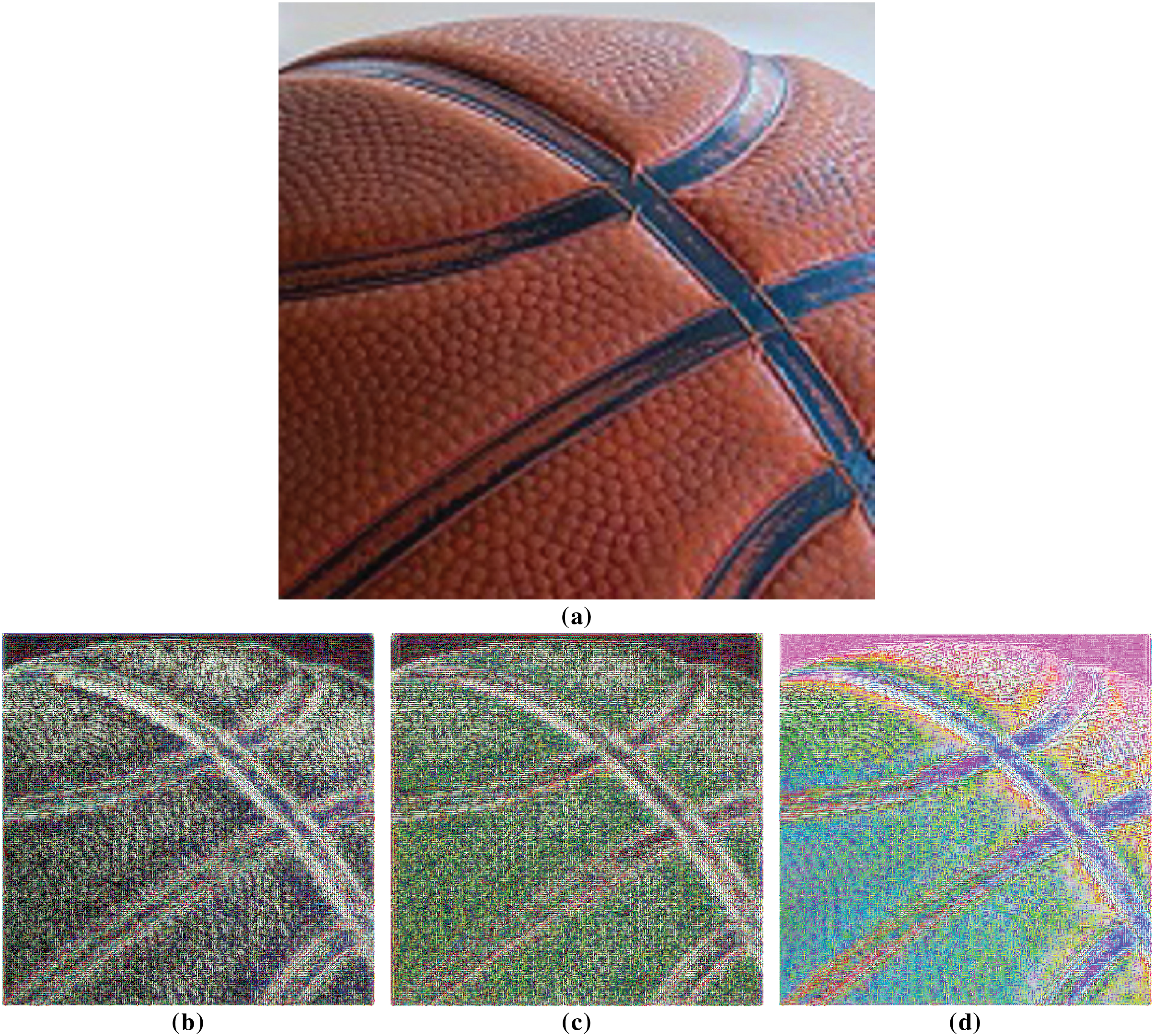
Figure 4: Image of a baseball from General100 validation subset (im_100.png) and corresponding contrast-enhanced difference maps (original minus SR reconstruction) using models trained on the BSDS300 dataset: (a) original image, (b) SR reconstruction—model trained with λs = 1, (c) SR reconstruction—model trained with λs = 0, (d) SR reconstruction—model trained with λs = 2

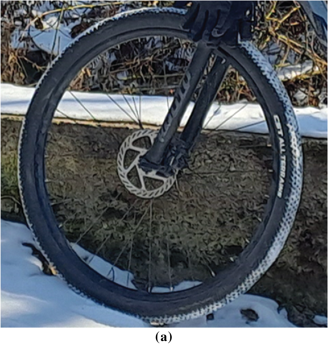
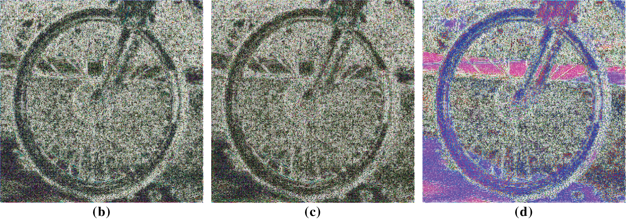
Figure 5: Image of an author’s photo of a bike (20250220_121442.png) and corresponding contrast-enhanced difference maps (original minus SR reconstruction) using models trained on the BSDS300 dataset: (a) original image, (b) SR reconstruction with λs = 1, (c) λs = 0, (d) λs = 2

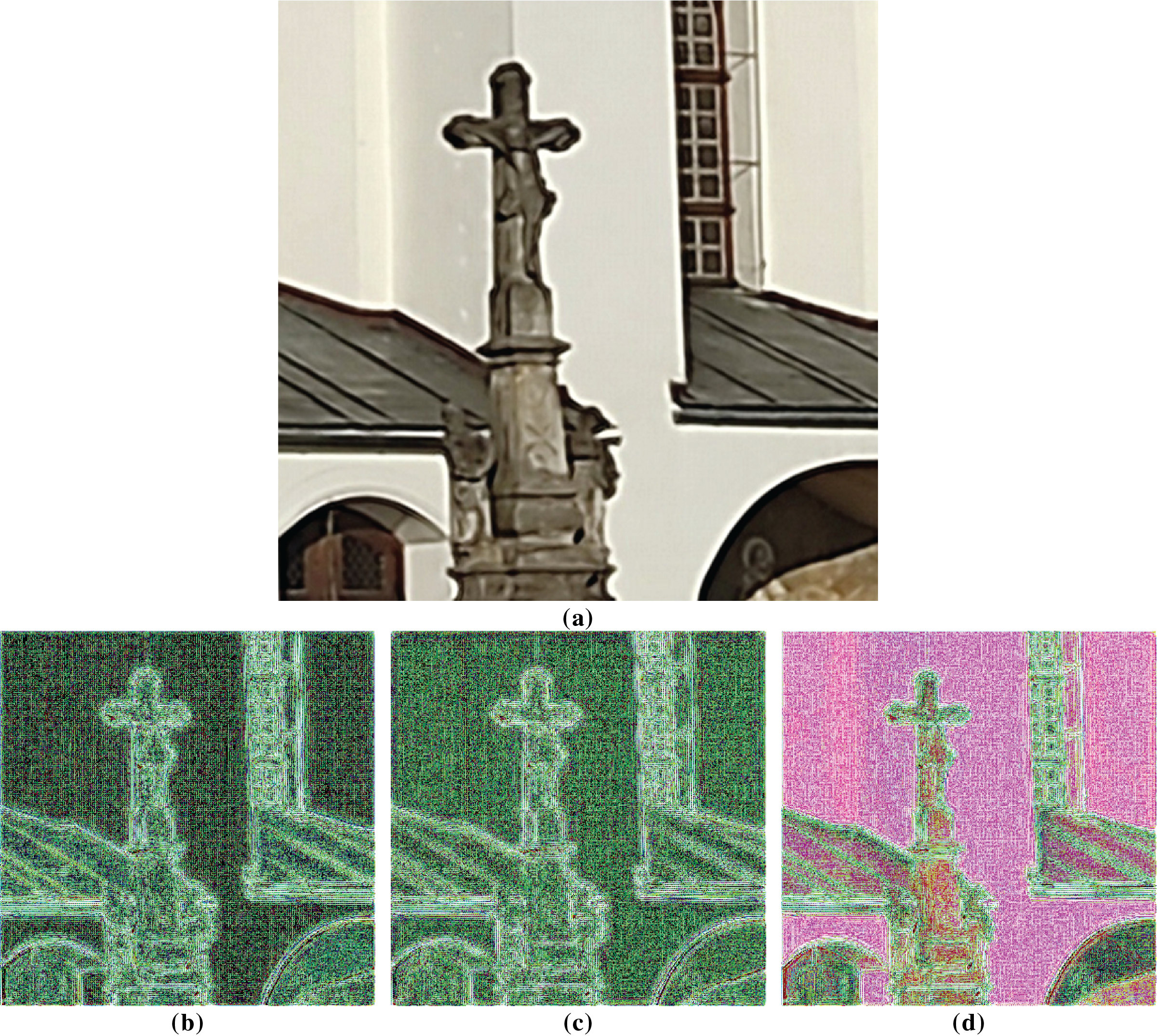
Figure 6: Image of an author’s photo of a cross in front of the church of John the Baptist in Velké Losiny (20250220_150700.png) and corresponding contrast-enhanced difference maps (original minus SR reconstruction) using models trained on the BSDS300 dataset: (a) original image, (b) SR reconstruction with λs = 1, (c) λs = 0, (d) λs = 2

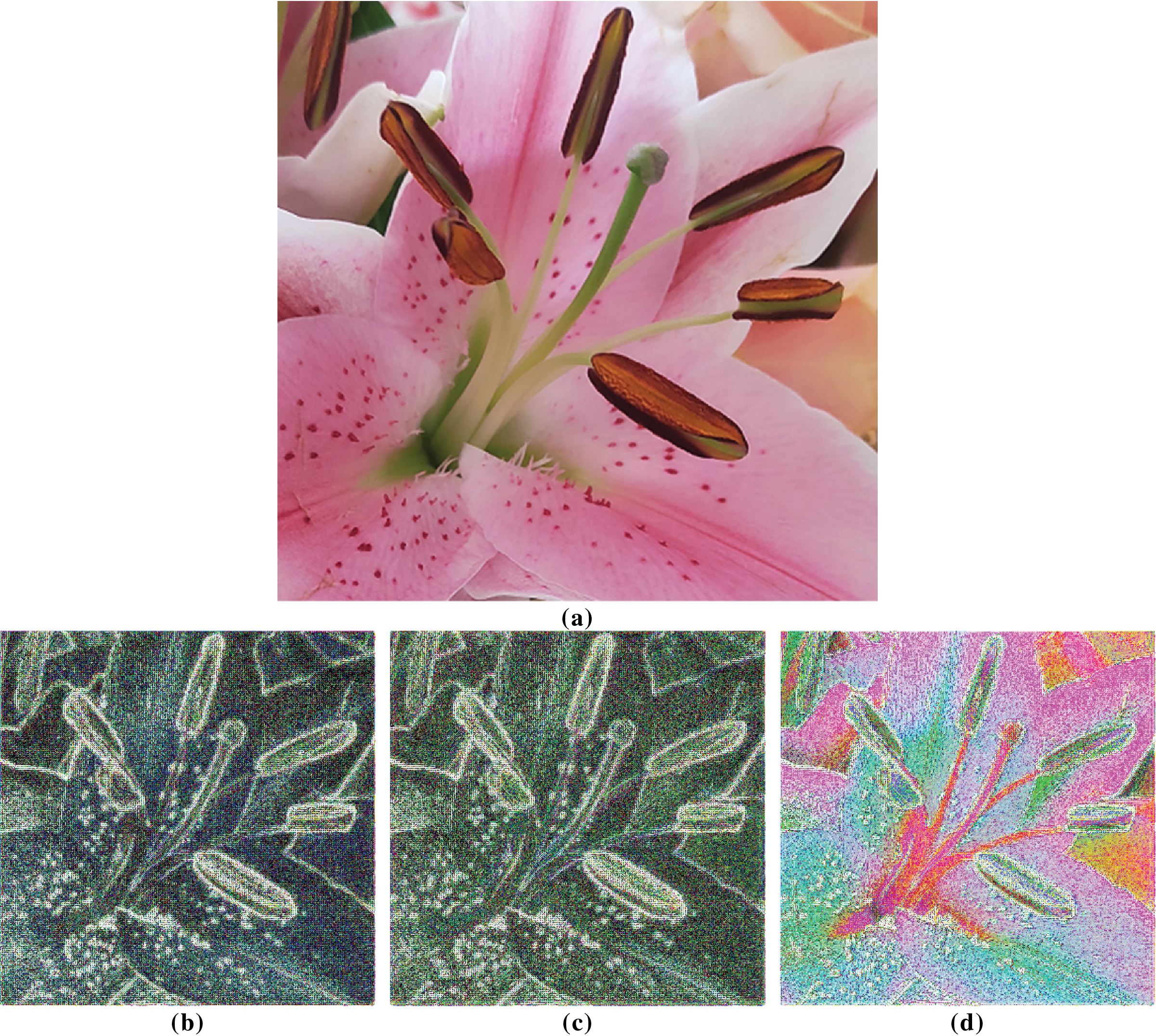
Figure 7: Image of an author’s photo of a pink flower (20250217_151002.png) and corresponding contrast-enhanced difference maps (original minus SR reconstruction) using models trained on the BSDS300 dataset: (a) original image, (b) SR reconstruction with λs = 1, (c) λs = 0, (d) λs = 2

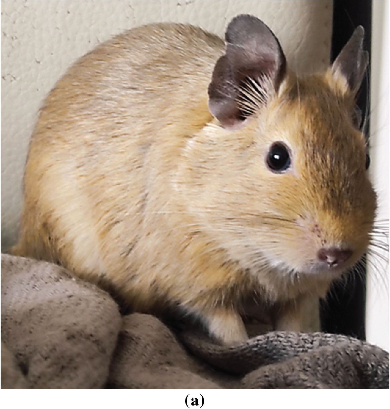
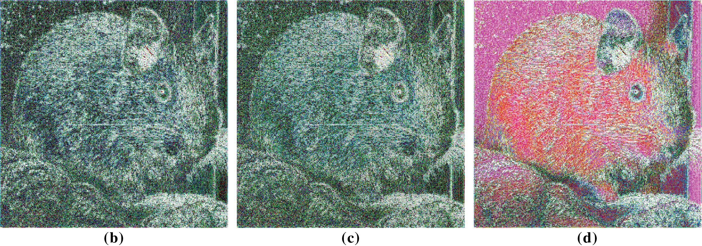
Figure 8: Image of an author’s photo of a common degu (20250503_141137.png) and corresponding contrast-enhanced difference maps (original minus SR reconstruction) using models trained on the BSDS300 dataset: (a) original image, (b) SR reconstruction with λs = 1, (c) λs = 0, (d) λs = 2

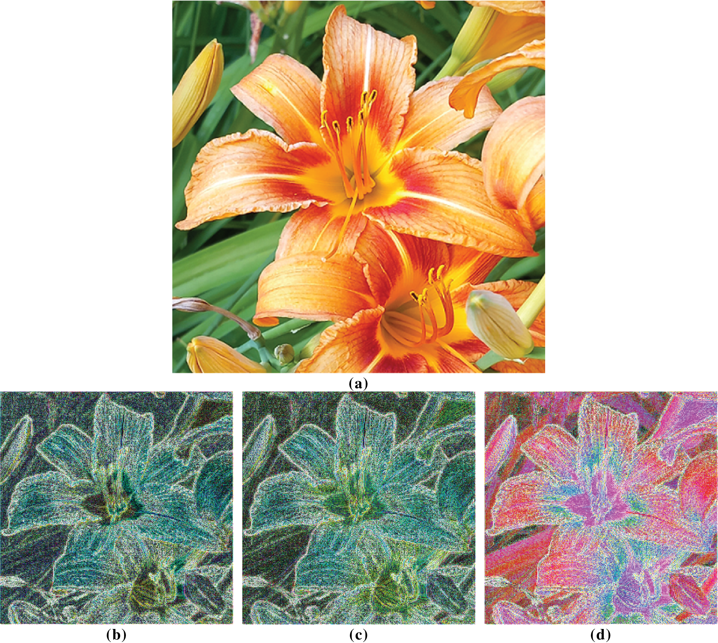
Figure 9: Image of an author’s photo of an orange flower (20230622_175044.png) and corresponding contrast-enhanced difference maps (original minus SR reconstruction) using models trained on the BSDS300 dataset: (a) original image, (b) SR reconstruction with λs = 1, (c) λs = 0, (d) λs = 2

Models not including the SSIM loss in their components (λs = 0) generally achieve higher scores in the PSNR evaluation metric, because it is directly derived from MSE, by 1787 dB in mean in comparison with models minimised with LSSIMN (λs = 1) and by 2.518 dB in comparison with models minimised with LSSIM (λs = 2). The average improvement of the resulting SSIM value on the validation set when including LSSIMN (λs = 1) was 2.88% for all experiments in comparison with leaving it out (λs = 0), 2.67% when not normalising it (λs = 2) in comparison with leaving it out (λs = 0) and the improvement when using LSSIMN (λs = 1) over LSSIM (λs = 2) in the resulting SSIM value was by 0.218% and PSNR increased by 0.73 dB.

The highest SSIM value of overall experiments reached 93.09% on the SR algorithm trained with LSSIMN (λs = 1) on the BSDS dataset.

4.1 Qualitative Comparison

Since the nominal difference in SSIM is in the order of hundredths, these differences are relatively difficult to observe. However, the qualitative comparison shown in Figs. 4–9 indicates that the inclusion of the LSSIMN (λs = 1) loss component contributes to slightly improved edge sharpness and better texture preservation, while leaving it out (λs = 0) causes slightly noisier results. Moreover, the detailed analysis in Section 3.2 confirms the difference. Visually, it is not possible to compare models trained by minimising the LSSIMN (λs = 1) and LSSIM (λs = 2) with the naked eye, but the contrast-enhanced maps in Figs. 4(b–d)–9(b–d) make this difference visible, and Table 4 indicates the quantitative differences in selected Figs. 4–9.

The highest value of each metric for each image is highlighted in bold. The LPIPS score showed significant variability across different model configurations, with no consistent pattern emerging across images. This variation is consistent with the trends observed during the validation phase and suggests that the perceptual similarity, as measured by LPIPS, is highly sensitive to the weights on which it was trained (SqueezeNet, AlexNet, and VggNet). In contrast, the PSNR metric tended to reach its maximum when the model was trained without including any LSSIM variant (λs = 0), specifically in four out of six cases. However, in two cases, the highest PSNR values were obtained when the model minimised the normalised structural similarity loss LSSIMN (λs = 1). The SSIM metric consistently reached its highest values, and in the case of the model trained with the normalised loss LSSIMN (λs = 1), this trend was uniform across all images.

While all three of the Super-Resolution models achieve high-quality results, subtle differences can be observed, especially in rendering edges and fine details like a continuation of lines. Figs. 4–9 present qualitative comparisons using test images that were included in neither the training nor validation subsets of the BSDS300 SR model to make sure that the evaluation is unbiased and does not suffer from data leakage. Selection was made manually to cover different visual characteristics, and no quantitative criteria or ranking were applied in the selection process. Fig. 4 is picked and cropped from the General100 validation dataset and Figs. 5–9 are photographs by the authors of this article, all of them are cropped to 400 × 400 px.

Figs. 4(b–d)–9(b–d) show contrast-enhanced difference images, i.e., pixel difference maps between reference images 4a–9a and corresponding reconstructions—outputs of SR algorithms trained with different λs parameters—subsequently processed by contrast enhancement using histogram equalisation for individual channels. Histogram equalisation visually increases the size of errors and thus improves the interpretability of differences at first glance and serves as a diagnostic tool for visual inspection. To maintain the ratio of brightness of the individual images and to allow for a better and more accurate comparison, all three individual images were first combined into one composite, on which the histogram equalisation was then performed. Brighter areas in these contrast-enhanced difference images indicate areas with a larger difference between the reconstructed and real ones. Dark areas correspond to areas where the reconstructed image matches the reference image. Light contours and textures reveal edge mismatches. Hue variations, i.e., places where colour is preserved in contrast-enhanced difference images, indicate distortion of the colour spectrum or incorrect colour reconstruction between individual RGB channels. From these difference images, it is evident that the images with the highest SSIM value (i.e., images reconstructed with the normalized loss LSSIMN (λs = 1)) achieve the smallest differences compared to the original image.

4.2 Comparison with Related Works

Huang’s research [14] that introduced LSSIM without normalisation reached similar results—increase in SSIM in contrary with the decrease in Root Mean Square Error RMSE when incorporating LSSIM. Without LSSIMSSIM reached the value of 0.855 in mean and RMSE reached the value of 0.176 in their experiments. With LSSIM incorporated in the composite loss function, SSIM reached 0.886 after the last epoch and RMSE reached 0.158. The improvement in image reconstruction results is noticeable in the figures provided in the paper.

From the perspective of using this loss function component, its importance has already been proven in Huang’s research. Still, the importance of normalisation, which ensures that the individual components of the loss function are in the same range of values, has not been considered before. Another recent contribution to the development of SR methods is the work by Gao et al. [26], who proposed a robust symmetrical and recursive transformer network for image super-resolution (SRTNet) and tested it on multiple benchmark datasets. Their model integrates a recursive feedback mechanism and a dual-branch design to improve the reconstructed images and to address the problem of computational cost. While their focus is on architectural innovation rather than loss function design, they also emphasise structural preservation as a key objective, indirectly aligning with our goal of LSSIM-based approaches. However, their work does not explore explicit LSSIM-based loss components or the effect of loss normalisation. Our research proved that normalising this component can bring even better results.

4.3 Next Steps

Further research steps may be aimed at experimenting with the setting of the λ weight coefficients of the composite loss function described in Eq. (11) and their influence on the resulting quality of the generated images, or the inclusion of adaptive weight settings during training or studying and comparing the effect of other loss component functions, similarly to Hybrid Perceptual Structural and Pixel-wise Residual (HyPSPR) [19]. It would also be possible to extend the experiments to other benchmark datasets to confirm the ability to perform better reconstruction on completely different images and use this component in training practical SR algorithms.

5  Conclusions

In this paper, we investigated the impact of loss function components on the outcome of Super-Resolution tasks. We newly presented the loss function component LSSIMN calculated from the normalised SSIM value between zero and one for better comparison and better scalability with other loss function components in the composite loss function minimised during the training of Super-Resolution models and found out it results in better quality images. This loss function is not generally applicable to a wide range of deep learning tasks, it is focused exclusively on image reconstruction, but we believe it is beneficial to the current state of knowledge.

When training Super-Resolution models, it is evident that including the normalised loss component LSSIMN in the overall loss function has an impact on the visual quality of the reconstructed images. Upscaling models using this function generate images that are visually more faithful to the original images for humans, specifically, higher fidelity of textures and edges is evident.

If the goal is to achieve a reconstruction that looks natural and is structurally consistent with the original images, LSSIMN has a significant role. However, if numerical pixel accuracy is a priority, e.g., for further algorithmic processing, then omitting LSSIMN may lead to better results in terms of pixel-wise accuracy.

Although the normalisation of the SSIM component is mathematically straightforward, our experiments demonstrate that it improves the compatibility between loss components and contributes to more efficient training and slightly better image reconstruction. The contribution of our research lies in the systematic analysis within a controlled experimental environment, which has not been explicitly addressed in previous works. We believe that our observations are relevant for future studies of loss function design in image reconstruction tasks.

Acknowledgement: We would like to hereby thank doc. Ing. Arnošt Veselý, CSc. for invaluable advice during writing this article.

Funding Statement: The results and knowledge included herein have been obtained owing to support from the following institutional grant. Internal Grant Agency of the Faculty of Economics and Management, Czech University of Life Sciences Prague, grant no. 2023A0004 (https://iga.pef.czu.cz/, accessed on 6 June 2025). Funds were granted to T. Novák, and A. Hamplová from the author team.

Author Contributions: The authors confirm contribution to the paper as follows: Conceptualisation, Adéla Hamplová; methodology, Adéla Hamplová; software, Adéla Hamplová; validation, Adéla Hamplová; formal analysis, Adéla Hamplová; investigation, Adéla Hamplová; resources, Adéla Hamplová, Tomáš Novák; data curation, Adéla Hamplová; writing—original draft preparation, Adéla Hamplová; writing—review and editing, Tomáš Novák, Miroslav Žáček, Jiří Brožek; visualisation, Adéla Hamplová, Jiří Brožek; supervision, Adéla Hamplová; project administration, Adéla Hamplová; funding acquisition, Adéla Hamplová. All authors reviewed the results and approved the final version of the manuscript.

Availability of Data and Materials: The code generated for this research is openly available on [normalised-SSIM-loss-SR] GitHub repository at [https://github.com/adelajelinkova/normalised-SSIM-loss-SR]. The datasets used for training the models are openly available at URL addresses: DIV2K [20] [https://data.vision.ee.ethz.ch/cvl/DIV2K/], BSDS300 [22] [https://www2.eecs.berkeley.edu/Research/Projects/CS/vision/bsds/] and General 100 [21] [https://mmlab.ie.cuhk.edu.hk/projects/FSRCNN.html]. Pre-trained models and logs, from which results were calculated, are available at [https://drive.google.com/drive/folders/1-lvrKZ9koByt323fN2yCqt7pqJf9oK4L?usp=sharing] (accessed on 6 June 2025.)

Ethics Approval: Not applicable.

Conflicts of Interest: The authors declare no conflicts of interest to report regarding the present study.

Appendix A Perceptual Loss Block Grid Search: Appendix A provides a list of options and an interpretation guide to the convolutional blocks available in VGG19 network that can be selected during minimising perceptual loss. Each block extracts features at a different level of abstraction—lowest layers capture low-level features such as lines, edges, etc., and last layer interprets the whole objects.

The list of blocks and their interpretations is as follows:

To identify the most suitable layer configuration for our task, we performed a grid search over multiple block combinations using the IRN model and the DIV2K_1000 dataset. We evaluated combinations of VGG19 feature layers that correspond to different levels of the network hierarchy, including the pairs block1_conv2–block4_conv4 combining lower-middle feature with higher-middle feature, block2_conv2–block5_conv2 combining lower-middle feature with the highest-level feature, block3_conv2–block4_conv4 combining two middle-level features, and block4_conv4–block5_conv4 combining higher-middle features with top-level features. The results of this comparison are provided in Table A2.

References

1. Li W, Liu H, Wang J. A deep learning method for denoising based on a fast and flexible convolutional neural network. IEEE Trans Geosci Remote Sens. 2021;60(2):1–13. doi:10.1109/TGRS.2021.3073001. [Google Scholar] [CrossRef]

2. Ignatov A, Romero A, Kim H, Timofte R, Ho CM, Meng Z, et al. Real-time video super-resolution on smartphones with deep learning, mobile AI 2021 challenge: report. In: Proceedings of the 2021 IEEE/CVF Conference on Computer Vision and Pattern Recognition Workshops (CVPRW); 2021 Jun 19–25; Nashville, TN, USA. doi:10.1109/CVPRW53098.2021.00287. [Google Scholar] [CrossRef]

3. Wang Z, Ye M, Yang F, Bai X, Satoh S. Cascaded SR-GAN for scale-adaptive low resolution person re-identification. In: Proceedings of the 27th International Joint Conference on Artificial Intelligence (IJCAI); 2018 Jul 13–19; Stockholm, Sweden. doi:10.24963/ijcai.2018/541. [Google Scholar] [CrossRef]

4. Yu X, Butler SK, Kong L, Milbeck BAF, Barajas-Olalde C, Burton-Kelly ME, et al. Machine learning-assisted upscaling analysis of reservoir rock core properties based on micro-computed tomography imagery. J Pet Sci Eng. 2022;219(9):1–26. doi:10.1016/j.petrol.2022.111087. [Google Scholar] [CrossRef]

5. Tsai RY, Huang TS. Multiframe image restoration and registration for spaceborne sensors. Adv Comput Vis Image Process. 1984;1:317–39. doi:10.1016/j.rinp.2021.103991. [Google Scholar] [CrossRef]

6. Crivellari A, Wei H, Wei C, Shi Y. Super-resolution GANs for upscaling unplanned urban settlements from remote sensing satellite imagery—the case of Chinese urban village detection. Int J Digit Earth. 2023;16(1):2623–43. doi:10.1080/17538947.2023.2230956. [Google Scholar] [CrossRef]

7. Tan W, Qin N, Zhang Y, McGrath H, Fortin M, Jonathan L. A rapid high-resolution multi-sensory urban flood mapping framework via DEM upscaling. Remote Sens Environ. 2024;301(4):113956. doi:10.1016/j.rse.2023.113956. [Google Scholar] [CrossRef]

8. Belharbi S, Sarraf A, Pedersoli M, Ayed I, McCaffrey L, Granger EF. CAM: full resolution class activation maps via guided parametric upscaling. In: Proceedings of the 2022 IEEE/CVF Winter Conference on Applications of Computer Vision (WACV); 2022 Jan 3–8; Waikoloa, HI, USA. doi:10.1109/WACV51458.2022.00378. [Google Scholar] [CrossRef]

9. Anh HK, Lee S, Jung SO. A CNN-based super-resolution processor with short-term caching for real-time UHD upscaling. IEEE Trans Circuits Sys I Reg Pap. 2024;71(3):1198–207. doi:10.1109/TCSI.2023.3346440. [Google Scholar] [CrossRef]

10. Xiao M, Zheng S, Liu C, Wang Y, He D, Ke G, et al. Invertible image rescaling. In: Proceedings of the 16th European Conference on Computer Vision (ECCV); 2020 Aug 23–28; Glasgow, UK. doi:10.1007/978-3-030-58452-8_8. [Google Scholar] [CrossRef]

11. Xiao M, Zheng S, Liu C, Lin Z, Liu TY. Invertible rescaling network and its extensions. Int J Comput Vis. 2022;131(9):1–26. doi:10.1007/s11263-022-01688-4. [Google Scholar] [CrossRef]

12. Xu BN, Guo Y, Jiang LQ, Yu MJ, Chen J. Downscaled representation matters: improving image rescaling with collaborative downscaled images. In: Proceedings of the IEEE/CVF International Conference on Computer Vision (ICCV); 2023 Oct 1–6; Paris, France. doi:10.1109/ICCV51070.2023.01124. [Google Scholar] [CrossRef]

13. Johnson J, Alahi A, Li FF. Perceptual losses for real-time style transfer and super-resolution. In: Proceedings of the 14th European Conference on Computer Vision (ECCV); 2016 Oct 11–14; Amsterdam, The Netherlands. doi:10.1007/978-3-319-46475-6_43. [Google Scholar] [CrossRef]

14. Huang Y, Song R, Xu K, Ye X, Li C, Chen X. Deep learning-based inverse scattering with structural similarity loss functions. IEEE Sens J. 2021;21(4):4900–7. doi:10.1109/JSEN.2020.3030321. [Google Scholar] [CrossRef]

15. Wang Z, Bovik AC, Sheikh HR, Simoncelli EP. Image quality assessment: from error visibility to structural similarity. IEEE Trans Image Process. 2004;13(4):600–12. doi:10.1109/TIP.2004.819325. [Google Scholar] [CrossRef]

16. Chollet F. Deep learning with python. 2nd ed. New York, NY, USA: Simon and Schuster; 2021. p. 73–80. [Google Scholar]

17. Ledig C, Theis L, Huszar F, Caballero J, Cunningham A, Acosta A, et al. Photo-realistic single image super-resolution using a generative adversarial network. In: Proceedings of the 2017 IEEE Conference on Computer Vision and Pattern Recognition (CVPR); 2017 Jul 21–26; Honolulu, HI, USA. doi:10.1109/CVPR.2017.19. [Google Scholar] [CrossRef]

18. Simonyan K, Zisserman A. Very deep convolutional networks for large-scale image recognition. In: Proceedings of the 3rd International Conference on Learning Representations (ICLR); 2015 May 7–9; San Diego, CA, USA. doi:10.48550/arXiv.1409.1556. [Google Scholar] [CrossRef]

19. Singla S, Bohat VK, Aggarwal M, Mehta Y. Hybrid perceptual structural and pixelwise residual loss function based image super-resolution. In: Proceedings of the 2024 3rd International Conference for Innovation in Technology (INOCON); 2024 Mar 1–3; Bangalore, India. doi:10.1109/INOCON60754.2024.10511465. [Google Scholar] [CrossRef]

20. Augustsson E, Timofte R. NTIRE 2017 challenge on single image super-resolution: dataset and study. In: Proceedings of the 2017 IEEE Conference on Computer Vision and Pattern Recognition Workshops (CVPRW); 2017; Honululu, HI, USA. doi:10.1109/CVPRW.2017.150. [Google Scholar] [CrossRef]

21. Zeyde R, Elad M, Protter M. Dataset: General100. doi:10.57702/m4tsd5mf. [Google Scholar] [CrossRef]

22. Martin D, Fowlkes C, Tal D, Malik J. A database of human segmented natural images and its application to evaluating segmentation algorithms and measuring ecological statistics. In: Proceedings of the Eighth IEEE International Conference on Computer Vision (ICCV); 2001 Jul 7–14; Vancouver, BC, Canada. doi:10.1109/ICCV.2001.937655. [Google Scholar] [CrossRef]

23. Zhang R, Isola P, Efros AA, Shechtman E, Wang O. The unreasonable effectiveness of deep features as a perceptual metric. In: Proceedings of the IEEE Conference on Computer Vision and Pattern Recognition (CVPR); 2018 Jun 18–22; Salt Lake City, UT, USA. doi:10.1109/CVPR.2018.00068. [Google Scholar] [CrossRef]

24. Barron JT. A general and adaptive robust loss function. In: Proceedings of the IEEE Conference on Computer Vision and Pattern Recognition (CVPR); 2019 Jun 16–20; Long Beach, CA, USA. doi:10.48550/arXiv.1701.03077. [Google Scholar] [CrossRef]

25. Blau Y, Michaeli T. The perception-distortion tradeoff. In: Proceedings of the 2018 IEEE/CVF Conference on Computer Vision and Pattern Recognition (CVPR); 2018 Jun 18–23; Salt Lake City, UT, USA. doi:10.1109/CVPR.2018.00652. [Google Scholar] [CrossRef]

26. Gao M, Sun J, Li Q, Khan MA, Shang J, Zhu X, et al. Towards trustworthy image super-resolution via symmetrical and recursive artificial neural network. IEEE Img Vis Comput. 2025;158(21):105519. doi:10.1016/j.imavis.2025.105519. [Google Scholar] [CrossRef]