
 Submit a Paper
 Propose a Special lssue
 Open Access
ARTICLE

Using Time Series Foundation Models for Few-Shot Remaining Useful Life Prediction of Aircraft Engines
Computer Engineering and Electronics Department, Faculty of Sciences, University of Cantabria, Santander, 39005, Spain
* Corresponding Author: Ricardo Dintén. Email:
Computer Modeling in Engineering & Sciences 2025, 144(1), 239-265. https://doi.org/10.32604/cmes.2025.065461
Received 13 March 2025; Accepted 26 June 2025; Issue published 31 July 2025
 View Full Text
 Download PDF
Abstract
Predictive maintenance often involves imbalanced multivariate time series datasets with scarce failure events, posing challenges for model training due to the high dimensionality of the data and the need for domain-specific preprocessing, which frequently leads to the development of large and complex models. Inspired by the success of Large Language Models (LLMs), transformer-based foundation models have been developed for time series (TSFM). These models have been proven to reconstruct time series in a zero-shot manner, being able to capture different patterns that effectively characterize time series. This paper proposes the use of TSFM to generate embeddings of the input data space, making them more interpretable for machine learning models. To evaluate the effectiveness of our approach, we trained three classical machine learning algorithms and one neural network using the embeddings generated by the TSFM called Moment for predicting the remaining useful life of aircraft engines. We test the models trained with both the full training dataset and only 10% of the training samples. Our results show that training simple models, such as support vector regressors or neural networks, with embeddings generated by Moment not only accelerates the training process but also enhances performance in few-shot learning scenarios, where data is scarce. This suggests a promising alternative to complex deep learning architectures, particularly in industrial contexts with limited labeled data.Keywords
In the context of Industry 4.0, predictive maintenance (PdM) emerges as a key component to optimize manufacturing processes by improving productivity and reducing costs. PdM harnesses the convergence of advanced technologies, such as the Internet of Things (IoT), real-time data analytics, and machine learning (ML) algorithms, to anticipate equipment failures before they occur. This enables industries to optimize maintenance plans, improve operational efficiency, and ensure the reliability of critical assets [1].
PdM mainly addresses three types of problems [2]: (1) anomaly detection, (2) failure diagnosis, and (3) prediction of the remaining useful life (RUL). Anomaly detection focuses on identifying potential failures that have recently occurred or are about to happen. Failure diagnosis seeks to determine the root cause of a problem, typically using root cause analysis (RCA) techniques. And RUL aims at estimating the time or number of operation cycles remaining before a system or component reaches the end of its operational life, making this one of the most challenging problems to be solved.
To address the problem of RUL prediction, two approaches are generally used: model-based methods and data-driven methods. The former relies on mathematical and physical principles and prior system knowledge to create predictive models. However, these methods can be complex, costly, and time-consuming due to the need for in-depth knowledge of the system. In contrast, data-driven methods explore the relationships between sensor data monitored and RUL values using historical data. But these, despite the numerous success cases mentioned in this survey [3], are also affected by certain inconveniences that hinder the building of accurate and reliable models while keeping the use of resources low. First, industrial assets operate under dynamically changing conditions, making it difficult to generalize prediction models [4]. Furthermore, the scarcity of labeled data poses a significant obstacle, as failures are rare events, and it is not always feasible to run the equipment until it fails to collect representative data [5]. In addition, when possible, the labeling work is labor-intensive, daunting, and time-consuming [3,6]. Finally, data sets are often unbalanced, with a high proportion of normal operating data and a low representation of failures, which can bias models [7].
In response to these limitations, recent advances in ML have introduced a range of innovative frameworks specifically designed to mitigate these challenges. One particularly effective strategy is the use of simulated or synthetic data, which enables the artificial replication of failure scenarios and the generation of full-lifecycle datasets in controlled environments. This approach not only reduces the reliance on costly and time-consuming real-world failure data but also facilitates model evaluation under diverse operational conditions without physically stressing the equipment [8]. Complementing this, semi-supervised learning methods—such as likelihood-based pseudo-labelling—have been developed to leverage large volumes of unlabelled sensor data while minimizing the need for manual annotation [9]. Hybrid approaches that integrate self-supervised and supervised learning techniques applied to incomplete lifecycle data have also demonstrated considerable effectiveness in extracting relevant degradation features from industrial environments [10]. Further strategies address the combined challenges of data scarcity and class imbalance through the integration of enhanced clustering techniques and synthetic oversampling [11]. To ensure model robustness across varying operational conditions, domain adaptation and transfer learning have been extensively explored to align data representations across multiple working environments, thereby improving generalizability [12]. Additionally, recent advances in uncertainty quantification have introduced probabilistic frameworks capable of estimating confidence in predictions, which is essential in safety-critical applications such as predictive maintenance [13]. Finally, an emerging direction combines several of these techniques within reinforcement learning-based frameworks. Recent studies have integrated synthetic data generation through data diffusion, Bayesian deep learning for uncertainty estimation, and active learning for sample selection, achieving significant improvements in prediction accuracy and reducing uncertainty by 15%–42% [14].
Building upon these trends, the necessity to enhance generalization capabilities and reduce labeling costs has catalyzed interest in n-shot learning paradigms, including few-shot, one-shot, and zero-shot learning. Few-shot learning typically leverages transfer learning (use a pretrained model [15]) or meta-learning techniques to train models that can recognize new classes using only a handful of labeled examples, whereas one-shot learning requires just a single labeled instance, and zero-shot learning, none.
Foundation models (FMs) are a class of deep learning (DL) models that are pretrained on vast amounts of data, thus equipped with a wide range of general knowledge and patterns. To this end, these models serve as a versatile starting point for various tasks across different domains. These models have proven to be useful in predicting future values in time series, classifying, detecting anomalies, filling in missing data, or generating synthetic time series that mimic real data for simulation tasks [15]. Additionally, they are valuable for interpreting model outcomes and identifying root causes [16].
In this paper, we explore the use of TSFM as a means to reduce the reliance on large labeled datasets and to enable the development of accurate predictive models with lower computational and energy demands [17]. TSFMs offer a robust, pretrained basis for extracting relevant features from time series data, allowing for the construction of simple, competitive predictors with minimal training data. By leveraging the representational power of TSFMs, we aim to promote model reuse, minimize dataset-specific preprocessing—often time-consuming and detrimental to generalizability—and enhance robustness in real-world industrial scenarios, where failure events are scarce.
More specifically, in this work, we experimentally assess the potential of a hybrid architecture that leverages the feature extraction strengths of TSFMs in conjunction with lightweight, resource-efficient ML algorithms. To this end, we design and conduct four experiments using the CMAPSS dataset to determine whether such a combination can:
• Match or surpass the predictive accuracy typically associated with DL models in time series regression problems, and significantly reduce training times compared to deep architectures based on recurrent or attention-based mechanisms.
• Minimize the preprocessing tasks by restricting data preparation to the essential steps required by the learning algorithm, relying on the ability of FM to manage dynamic behaviors and noisy data present in real-world scenarios.
• Utilize a reduced amount of labeled training data for building effective predictors, thereby mitigating the impact of the limited availability of annotated failure cases typically found in real-world industrial environments.
The performance of the proposed architecture is compared against 22 existing ML and DL models for RUL prediction on the CMAPSS dataset, selected from the recent literature.
This paper is organized as follows: Section 2 provides a background about artificial intelligence (AI) strategies followed to estimate the RUL, motivating the need and opportunity of using FM for this goal. Section 3 describes the methodology followed in this research. Section 4 details the experimentation conducted on the CMAPSS dataset, specifying the preprocessing tasks performed, the setting of models built, and their evaluation under the following metrics: RMSE, score, training time, and inference time. Section 5 discusses the findings of this study highlighting scenarios in which TSFM could be a promising alternative. Finally, Section 6 draws the conclusions of the paper and the next steps in our research.
Over the past decade, sensorisation and the adoption of AI techniques have revolutionized predictive maintenance, transforming the industrial sector significantly. The number of research surveys, both general and topic-specific, on PdM is vast, highlighting the importance of this field [2,18,19].
In the literature, we find PdM applications that employ all kind of AI approaches-supervised, unsupervised, and reinforcement learning-to analyze the large volume of data captured by real-time condition monitoring systems [20]. Within each paradigm, different algorithms from the ML and DL arena have been successfully applied. For instance, Li et al. [21] focused on the importance of accurately predicting the RUL of lithium-ion batteries using different algorithms. Their experimentation yielded that RNN (Recurrent Neural Network) and CNN (Convolutional Neural Network) present a good performance and ability for information extraction; SVR (Support Vector Regression) and ELM (Extreme Learning Machine) exhibit a good online updating ability and fast prediction; and AR (Auto-Regression) was the simplest algorithm with acceptable accuracy. Others, such as Taşcı et al. [22] proposed a hybrid model for the RUL prediction before production lines stop. They used real-world high-dimensional data from IoT sensors, and among all the proposed methods, RF (Random Forests), an ensemble bagging method, turned out to perform best. Later, Dintén et al. [23] used transformers to assess their effectiveness in anomaly detection and failure prediction, finding that the hybrid transformer-GRU (Gated Recurrent Unit) configuration delivers the highest accuracy, albeit at the cost of requiring the longest computational time for training. Also, Kim et al. [24] successfully implemented a transformer-based model to predict the RUL of lubricant used in operational rolling bearings. As Yu et al. [25] pointed out, when using transformers directly for failure prediction, the results often fail to meet expectations due to the sparsity of failure events within the datasets, leading to a model that learns temporally sparse features that do not adequately represent the complexity of failure prediction scenarios.
Despite the successes achieved so far, the intrinsic characteristics of industrial time series—being inherently temporal and capturing the dynamics of complex systems and processes—pose two major challenges in building robust and accurate predictive models. First, the scarcity of labeled datasets, which are also highly imbalanced due to the low frequency of failure events [5,15], often makes it difficult to construct a reliable and robust predictor, as pointed out by [25]. Second, the specificity of the behavior of each industrial asset limits the ability of the models to generalize. As previously mentioned, this has led the scientific community to propose innovative solutions to tackle these challenges, being one of these to develop adaptive approaches capable of transferring knowledge across different systems and operating conditions. Here is where TSFMs come into play–large AI models inspired by LLMs such as BERT [26] and GPT-3 [27], but specifically adapted for time series analysis [28]. One of their key advantages is that these models can be fine-tuned or adapted to specific tasks with relatively small amounts of task-specific data (few-shot learning) [29].
Recently, LLMs combining time series with textual prompts have achieved promising performance in TSFM. One approach represents time series as patches and leverages pretrained models for prediction [15]. Another research direction focuses on aligning embeddings between time series and textual data. This is the case of TimeCMA [30] that proposes a framework that uses dual-modality coding, combining time series embeddings generated with a transformer with embeddings obtained from textual cues in a pretrained LLM, improving accuracy and reducing computational costs. The transformer time-series attention is local and variable-specific, whereas LLM textual attention is universal and captures global dependencies between variables. Another proposal is TGForecaster [31], a robust baseline model that fuses textual cues, such as channel descriptions and dynamic news, and time series data using cross-attention mechanisms. Another approach is taken by TimeLLM [29] that adapts LLMs for time series forecasting by transforming time series into text prototypes and using the prompt-as-prefix technique to guide the transformation with natural language instructions. Other strategies convert the numerical input and output into prompts, and the forecasting task is framed in a sentence-to-sentence manner, making it possible to directly apply language models for forecasting purposes, such as PromptCast [32]. Finally, other models entirely rely on textual information for forecasting [33].
Subsequently, LLMs designed exclusively for time series data emerged, with Moment [34] being an outstanding example. Moment is a family of high-capacity transformer models pretrained on extensive time series datasets from diverse domains using a masked time series prediction task. In contrast to TimeCMA and TimeLLM, which may struggle with modelling long-term dependencies and capturing multi-scale temporal variations, Moment takes advantage of advanced pretraining techniques on large time series corpora, resulting in more robust and generalisable representations. Furthermore, its masked time series prediction task enhances the model’s ability to handle missing and noisy data, challenges frequently encountered in industrial applications. These capabilities enable Moment to surpass previous models in accuracy and adaptability across various time series analysis tasks, including forecasting, classification, and anomaly detection. Moreover, while the majority of the TSFM focuses on time series forecasting, Moment also offers representational learning, which allows users to obtain the values of the latent space where the most important characteristics of the time series are captured, making it a good feature extraction method that requires no training. This was the main reason for selecting this TSFM for our benchmark.
Another multipurpose model that covers forecasting, classification, regression or embedding generation is TOTEM [35]. TOTEM explores time series unification through discrete tokens instead of patches as used in allM4TS [36] and LLM4TS [37]. Its VQVAE (Vector Quantized Variational Autoencoders) backbone learns a fixed codebook of tokens over a multi-domain corpus of time series data independently from the training of any downstream model. This disentangles the choice of data representation from the choice of task-specific architecture and permits the learning of representations from a large, diverse set of data, which aids in zero-shot generalization. However, as far as we know, the authors have not yet published a pretrained version of the model.
Modern DL architectures such as transformers are revolutionizing the world of AI and time series predictions thanks to the multi-head self-attention mechanism introduced in [38], which can capture really complex non-linear relationships in the data and retain long-term relationships in sequences. However, the training of this kind of architecture requires a vast amount of data and extremely powerful specific hardware (such as GPUs, NPUs, or TPUs), making it very costly and time-consuming when compared to traditional ML models. This makes these models more difficult, when not impossible, to implement in fields like PdM, where the failure events are scarce in the datasets and cost reduction is of utmost importance.
Recently, TSFM have emerged, offering zero-shot forecasting and embedding generation for time series data. These models can help overcome the need to train these complex architectures from scratch. In this paper, we aim to experimentally validate whether a hybrid architecture that combines the feature extraction capabilities of TSFM with lightweight and less resource-intensive ML models can achieve the following goals:
• Improve or, at least, maintain the prediction performance achieved by DL models in time series regression tasks.
• Minimize the preprocessing tasks by restricting data preparation to the essential steps required by the learning algorithm.
• Minimize the amount of data needed to train the predictors (few-shot).
• Reduce training times compared to DL architectures based on recurrence and attention mechanisms.
To test our proposal, we designed the following benchmark. First, we chose a well-known RUL dataset, CMAPSS. Then, we selected four ML models from different paradigms: Random Forest, Light Gradient Boosting Machine, Support Vector Regressor, and a simple 1-hidden-layer Perceptron Neural Network. Next, we defined three scenarios to build a predictor with each model:
1. Using the full original data set.
2. Using the embeddings generated by Moment on the full dataset.
3. Using the embedding generated by Moment but only using a 10% of the original number of events (few-shot).
The 10% subset was selected based on a heuristic, experience-driven approximation, considering that the smallest dataset contains data of about 100 engines. Training with labeled data of 10 engines was deemed sufficient to simulate a realistic few-shot learning scenario while ensuring enough variability for model evaluation (see Experiment 3 in Section 4.5.3).
The predictive performance of the models is evaluated according to the RMSE and the score achieved with the test dataset. Furthermore, eighteen DL and ML models found in the literature for RUL prediction on this dataset were selected to do an honest comparison. Additionally, we measure the training time and inference time to know the computational cost and power consumption of each model.
Section 4 describes step-by-step the process followed and shows the measured metrics. Next, Section 5 discusses the results and draws the main insights extracted from the benchmark.
First, we graphically illustrate the process used to evaluate our approach with the CMAPSS dataset, from the data preparation phase to the result analysis (see Fig. 1). Based on this figure, we then describe the experimentation step by step.

Figure 1: Workflow followed to carry out this benchmark
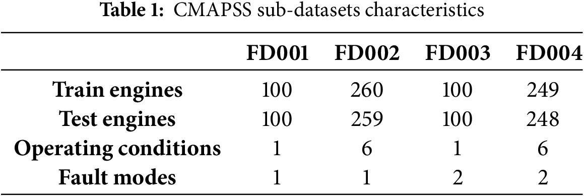
CMAPSS is a well-known synthetic benchmark dataset for the RUL prediction of a type of jet engine released by NASA for the PHM08 data challenge. It contains 4 sub-datasets composed by 26 numerical columns and a target variable representing the RUL. These variables are measured once every operational cycle, and the RUL column represents the number of operational cycles before the failure of the engine. The 4 sub-datasets contain some differences, such as varying working conditions or fault modes. These differences between the sub-datasets are summarized in Table 1.
4.1 Run-to-Failure Experiment Extraction
Each sub-dataset contains multiple trajectories (a.k.a. experiments), each one corresponding to a different engine. To ensure proper data inspection and analysis, it is essential to separate the experiments so that data from different engines do not overlap or mix during normalisation or sequence creation. In this case, the dataset provides a trajectory identifier, which we use to split the data accordingly.
Once each run-to-failure experiment was isolated, we analysed how the different variables evolve. Each plot, presented in Figs. A1–A4 in the Appendix, has 100 lines, each one representing the evolution of the feature for one turbofan engine in the FD001 sub-dataset during its useful life. These figures display the values of each variable, aligning the experiments at the end of the RUL (RUL = 0). The variables are categorized into four groups according to their behavior when the engine is near failure: variables with increasing trend, variables with decreasing trend, and the rest with random or stationary trend. These two last groups may not offer valuable information; in fact, they may add noise to the model, which negatively affects the predictions. However, as the aim is to reduce the preprocessing tasks to a minimum for both reducing costs and validating the capacity of FM to discard them, we will keep all the variables of the set.
Next, we carried out a minimal set of preprocessing techniques during the data preparation phase to ensure the data was suitable for model input. For this task, we adopted a straightforward three-step approach: (1) missing value imputation, (2) data normalisation, and (3) sequence creation.
First, we addressed missing value imputation, as ML models cannot process them directly. Since this dataset contains no null values, we bypassed this step without applying any modifications to the training data.
Next, we normalized the data so that the input features were in the same range of values. We applied Z-score normalization according to Eq. (1).
Finally, as we are working with time series data, the temporal evolution of the variables must be taken into account and not just the last event reported. Therefore, we had to provide the model with all the events that comprise each observation window. To achieve this, a sliding window transformation (see Fig. 2) was applied to the dataset. We chose two different values for the window size, 30 and 60. In [39], the authors found out that 30 was the optimal window size for this problem, however, since Moment is such a large and complex model, we tried 60 to check if the model could take advantage of the extra information added to the sequence.

Figure 2: Example of application of the sliding window algorithm with window size = 4 and stride = 1
As mentioned earlier, recent trends have focused on developing increasingly complex deep learning models to enhance prediction accuracy. However, this comes at the cost of higher computational demands for both training and inference, as well as the need for larger datasets. While the gain in accuracy may be desirable, these DL models are not always the best alternative for PdM problems, where the scarcity of failure data limits the generalisation capability of these models.
The arrival of TSFM, that have been proven to perform forecast, imputation, or representational learning in zero-shot scenarios successfully [34], can be a way to exploit the potential of the new complex transformer-based architectures without having to deal with costly training. Our proposal, see Fig. 3, uses a TSFM to create embeddings of the input data previously preprocessed that are used to train a simpler ML model. This strategy helps us reduce the training time and partially overcome the scarcity of failure data since these simpler models tend to require fewer samples to train (fewer parameters must be tuned).

Figure 3: Architecture of the proposed hybrid model. Preprocessed sequences are first encoded into embeddings using the TSFM, which are subsequently used to train a machine learning model. The model outputs are then post-processed using a moving average filter to smooth the predictions
Specifically, we compare four fundamental ML models trained on embeddings generated by the Moment model against the same models and several more advanced DL ones trained on the preprocessed dataset. We chose Moment TSFM because, as mentioned in Section 2, it beats almost any available competitor in forecasting accuracy, and it is the only open-source model, as far as we know, that offers a representational learning version that can be directly used for embedding creation. Moreover, this does not require the time or sampling frequency to be specified, which is particularly useful for the CMAPSS dataset, whose events do not include the time, but the operating cycle number.
The training and inference of each model was performed in a two-step process where the TSFM first converts two-dimensional sequences into a one-dimensional embedding vector that can be used as input for the ML models; and then, the training dataset converted to embeddings, along with the original RUL values, is used to train each ML model.
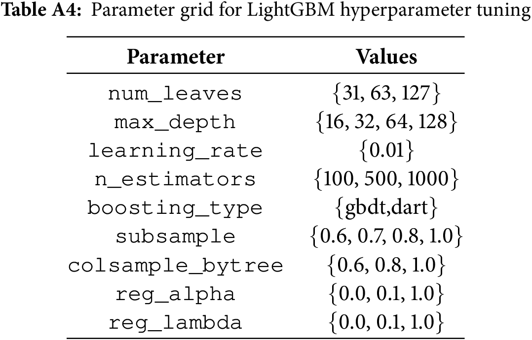
We chose the following four ML models: RF, SVR, NN and LGBM. Each model was tuned using an exhaustive grid search over the hyperparameter ranges specified in Tables A1–A4, respectively, in combination with 5-fold cross-validation. This strategy was adopted to ensure a robust hyperparameter optimization process and to minimize the variability introduced by random parameter initialization. Grid search systematically explores a wide set of values for each hyperparameter, and has been proven effective in identifying optimal configurations [40,41]. Meanwhile, 5-fold cross-validation partitions the training set into five equal subsets, iteratively training the model on four folds and validating it on the remaining one. The average of the evaluation metrics over the five folds provides a more stable and reliable estimate of model performance, reducing the sensitivity to randomness in both the train-test data split and model initialization.
For the inference, the TSFM and the trained regressor were pipelined in a model wrapper that implements the Estimator interface of the sci-kit learn package so, the new data could be passed directly as a sequence to the wrapper. In addition, as a consequence of the fact that the predictions of the first models were unstable and noisy (see Fig. 4), we implemented a moving average to control the oscillations of the predictions and to reduce the error.

Figure 4: Predictions of the models for 9 experiments from FD004 dataset. Blue line represents the predicted values, orange line the smoothed predictions and green line the ground truth
This experimentation shows and compares the 32 models built using two common metrics, the Root Mean Squared Error (see Eq. (2)) and the score provided in the PHM08 data challenge, where the dataset was first published. The RMSE is the standard metric for regression tasks, and the score is an asymmetric metric specific to this problem that punishes overestimations more than underestimation which is formulated according to Eq. (3).
The results are analyzed through four distinct experiments, each designed to address the following research questions:
• Experiment 1: To what extent does the embedding strategy enhance the RMSE and score achieved by the ML models?
• Experiment 2: How well do the embedding-based models perform compared to the ML and DL models found in the literature? Is it possible to reduce the preprocessing tasks to the essential steps required by the learning algorithm?
• Experiment 3: How robust are the models trained under the few-shot learning paradigm?
• Experiment 4: How much time and power are saved by using ML techniques instead of DL models?
4.5.1 Experiment 1: Model Performance with and without Embeddings
First, we compare the results obtained by training the models using the data directly after normalization and sequence generation with those obtained using the Moment-generated embeddings. As can be observed in Table 2 our approach of using embeddings fails to improve the performance of tree-based models, i.e., Gradient Boosting Machine and Random Forest. However, it improves the RMSE of SVR models in the two more complex datasets, FD002 and FD004. It is also worth noting, see Table 3, that in other works such as [42] the authors get much worse RMSE using SVR and NN (rows 2 and 3). We think the authors used only the last event or an aggregation of the observation window as input for the models, whereas we used the whole observation window flattened. However, the authors describe this issue neither in their article nor in the reference to the code, thus it could not be verified.
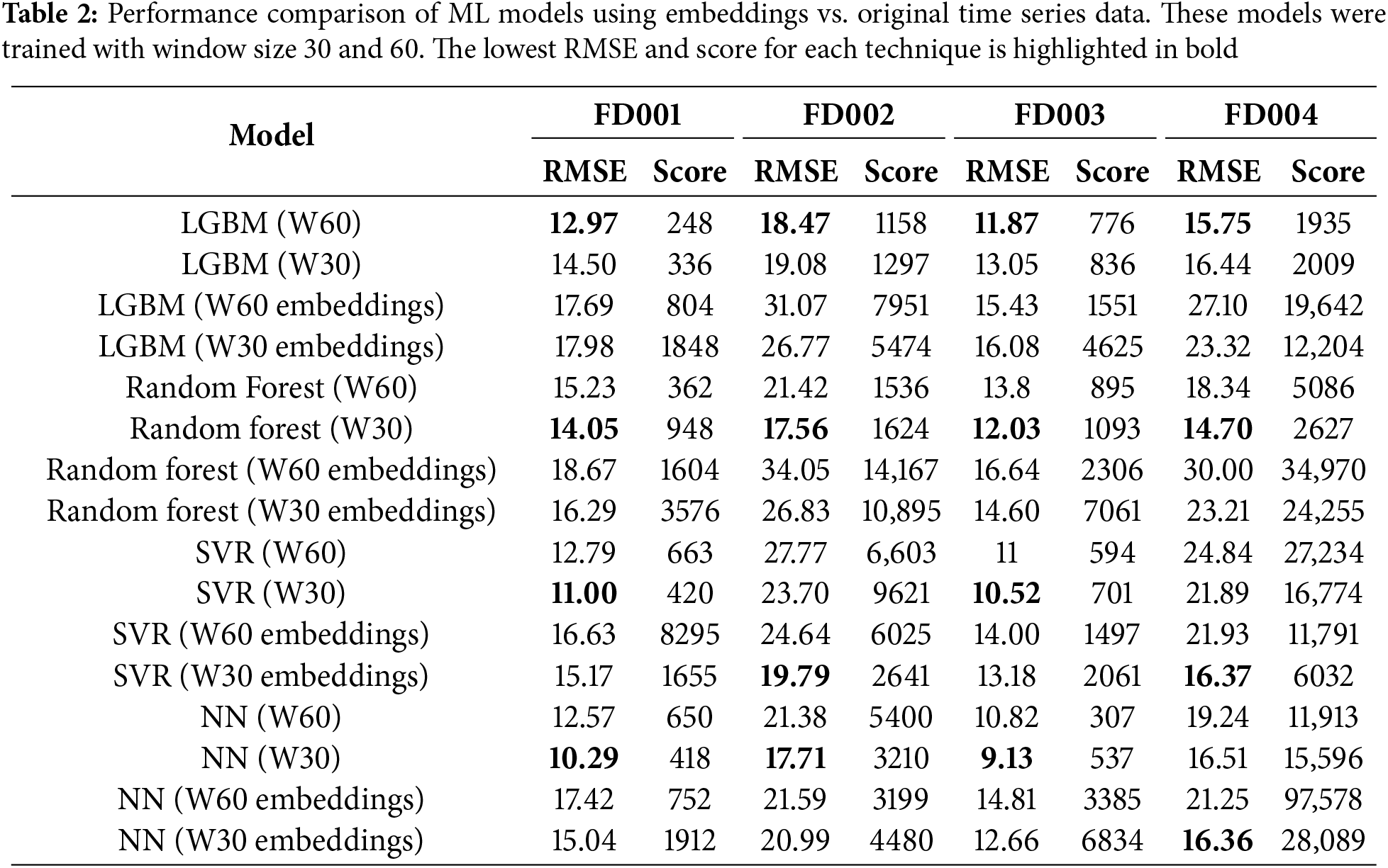
Regarding the score, the use of embeddings worsens its value. This is a twofold problem. First, the formula is computed as the sum of the scores for the last reading of each engine, which means that a bad prediction can greatly affect the final score. As seen in Fig. 4, the prediction suffers from many oscillations, which results in really high scores on certain engines. Second, we applied a moving average to the output of the models to control the oscillations. This helped us to reduce the RMSE. However, the score formula penalizes the overestimation of the RUL and, being RUL a monotonically decreasing function, the moving average produces a slight overestimation.
When analyzing the impact of the observation window size, the models trained using a sequence of length 30 provide better accuracy in most scenarios, which is in line with the study carried out in [39]. This proves that a longer observation window is not always beneficial and highlights the importance of carefully selecting the window size, even when using TSFM.
As a result of this first experiment, we can confidently say that the embedding strategy can help ML models to extract meaningful information in complex data scenarios. However, it is not appropriate for every kind of model, SVR being the model that takes greater advantage of the embedding generation, whereas the performance of the tree-based alternatives is negatively affected. Finally, the size of the sequence and the scoring metric can impact the usefulness of this approach.
4.5.2 Experiment 2: Embedding-Based ML Models vs. DL Models
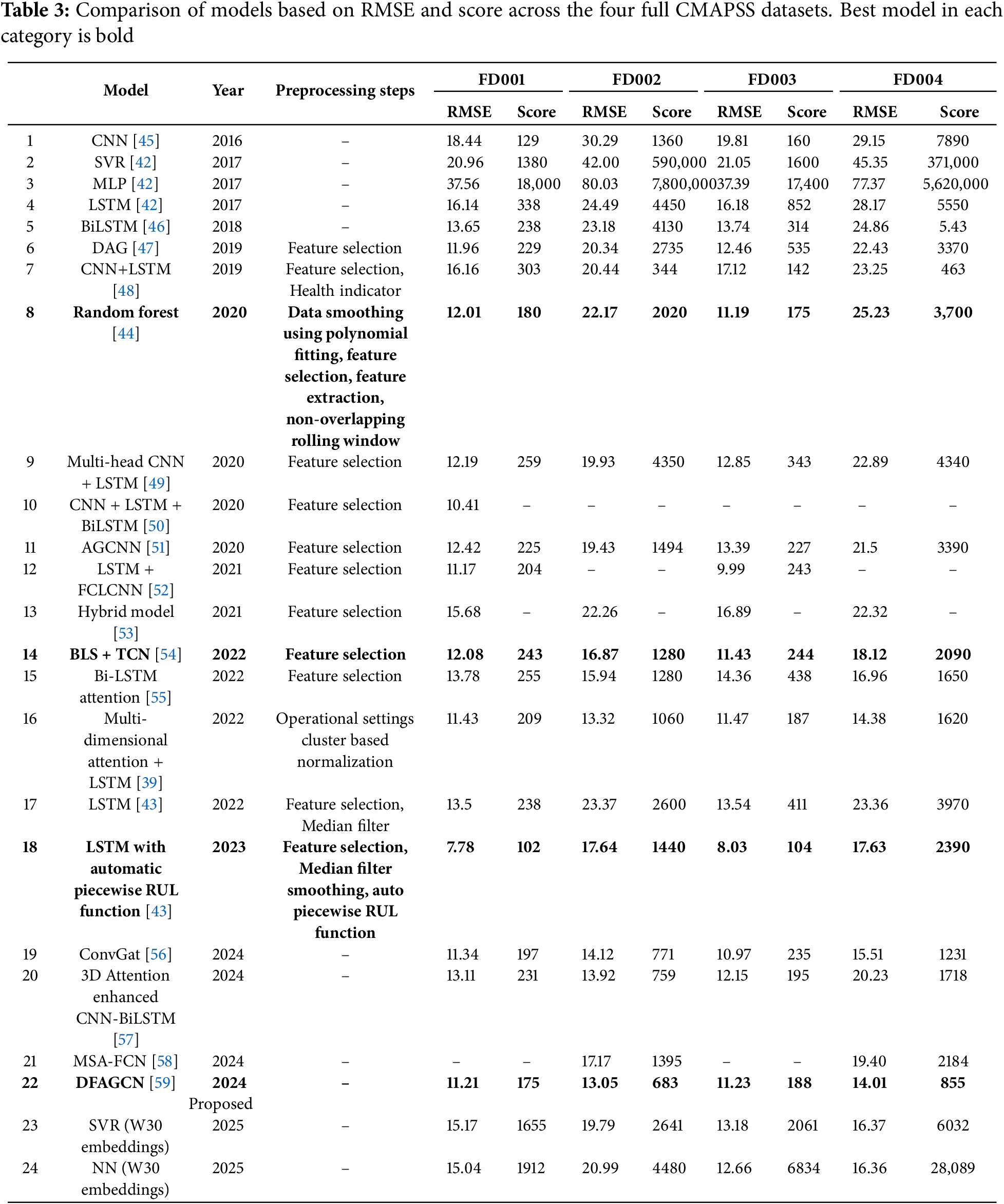
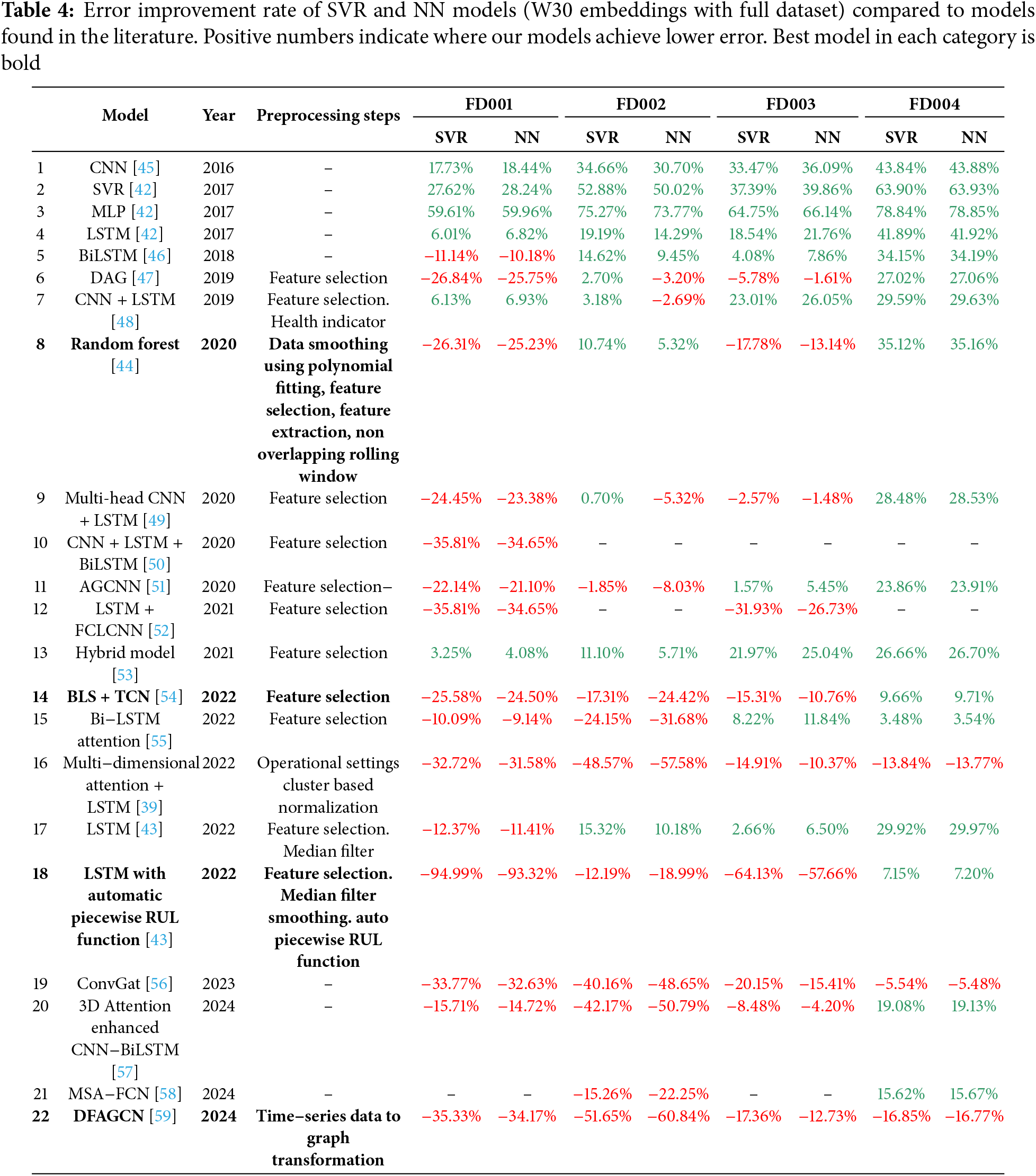
To carry out the performance comparison of models trained with ML techniques concerning more sophisticated proposals based on DL, we rely on 22 recent models found in the literature. All these predictors are presented in chronological order in Table 3-adapted from [43], and extended with additional references and our best proposed models, i.e., SRV and NN trained with embeddings and an observation window of 30 events. The table includes the type of model, preprocessing steps applied before training, and the RMSE and score obtained for each dataset. To maintain clarity, we have omitted the piecewise RUL function and the basic Z-score normalization, as these preprocessing steps are common to all works listed. In addition, to make the interpretation of the results easier, we include 4, which contains the difference in RMSE between our SVR and NN models as a percentage.
Models in Tables 3 and 4 can be grouped in 4 categories according to the kind of technique used for their training: machine learning, simple deep learning, hybrid deep learning, and hybrid attention learning. Our proposal outperforms all the ML models (see rows 2, 3, and 8) except for the Random Forest presented in [44], which achieved a better performance in the FD001 and FD003 datasets by using a specific preprocessing.
Regarding simple DL models (see rows 1, 4, 17, 18), our approach beats almost every model, especially in FD002 and FD004 datasets, except the LSTM used in [43] (see row 18). This is because it uses an automatic piecewise RUL function to choose the upper limit of the RUL (MaxRULValue), which reduces the maximum RUL value from 130 (the standard value for this problem) to around 80. This change artificially reduces the RMSE regardless of the model architecture employed. However, this error reduction occurs only in absolute terms. If we compute
The hybrid DL models (see rows 6, 7, 10, 11, 13, 14, 19) outperform our approach on FD001, FD002, and FD003 and achieve a comparable performance to our proposal on FD004, except for ConvGAT (row 19), which also surpasses our model on FD004. All hybrid attention-based models (see rows 9, 15, 16, 20, 21, 22) outperform our proposal on FD001. Additionally, Multi-head CNN + LSTM (row 9) performs better on FD003; BiLSTM Attention (row 15) on FD002 and FD004; 3D Attention-enhanced CNN-BiLSTM (row 20) on FD002, FD003, and FD004; and MSA-FCN (row 21) on FD002. Notably, both Multidimensional Attention and DFAGCN (rows 16 and 22) achieve lower errors across all four subsets. These two models outperform our approach on every subset and have two things in common. They combine attention mechanisms with other DL techniques and use specific preprocessing. On the one hand, the multi-dimensional attention LSTM combines the attention mechanism with a special normalization based on clusters of the operational settings of the engine. On the other hand, the DFAGCNN combines attention with graph representations, convolution, and recurrence in a complex architecture where the graph attention is used to dynamically select features, the convolution to encode the input, and the recurrence to extract the temporal patterns. Both models showcase an outstanding performance with RMSE values between 10% and 57% lower than our models in the case of the multi-dimensional attention LSTM and between 12% and 60% for the DFAGCNN (see Table 4). However, this comes at the cost of having high complexity models, which imply significantly longer training times and larger datasets to achieve that performance level, as we show in the Section 4.5.4.
By analyzing the model predictions, it can be observed (in Fig. 4) that the predicted values heavily oscillate around the actual value, which may be caused by the noise introduced during the zero-shot embedding creation. This indicates that when the algorithm can learn from the original data, embeddings can degrade its predictive performance. Conversely, if the algorithm cannot handle datasets with high dimensionality and variability to extract meaningful patterns from the original data, the use of embeddings has a positive impact despite the oscillations of the model predictions.
In summary, this second experiment demonstrates that the simplest ML models trained on the embeddings generated by the TSFM can achieve the same level of performance as the most modern and complex hybrid DL models in some scenarios, especially on datasets with higher complexity, such as FD002 and FD004 subsets.
Moreover, it is worth noting that our hybrid models using embeddings achieve comparable results to those obtained by state-of-the-art models that rely on dataset-specific preprocessing strategies, despite not requiring any tailored preprocessing beyond basic normalization and sequencing (see for instance rows 7, 8, 9, 15, 17).
4.5.3 Experiment 3: Few-Shot Learning
As mentioned earlier, the scarcity of failure data is a common challenge in predictive maintenance problems. To assess the ability to learn from fewer samples, we compared the perfomance of the models trained on embeddings vs. the ones trained on original time series values, using a 10% of the original training set. Table 5 shows that, once again, tree-based models struggle to learn effectively from embeddings, whereas SVR and NN perform better when the sample size is small if they are trained using embeddings. Notably, the RMSE of the SVR model worsens less than 4% when comparing the models trained using the embeddings of the full training set (see SVR 30W embeddings on Table 2) and continues to outperform simple DL models such as CNNs and LSTMs (see rows 1 and 4 in Table 3). On the other hand, the NN model experiences a more substantial performance drop of 15% in FD001, 6.71% in FD003, and 5.86% in FD004, but shows a 15% of improvement in the FD002 dataset.

After identifying SVR as the most effective ML technique in few-shot scenarios, we further investigate the impact of training set size on model performance using embeddings. Therefore, we carried out the training of models with the 5%, 10%, 15%, and 20% of the full dataset. The results, presented in Table 6, show that, with only 5% of the training data, the RMSE of the SVR model trained with embeddings increases by 11%, 1%, 9%, and 7% on FD001, FD002, FD003, and FD004, respectively.

It is worth noting that the model attains near-maximum performance using only 10% to 15% of the training data. Beyond this point, further increases in training size yield only marginal improvements, likely due to initialisation variability rather than meaningful gains in learning.
Finally, it must be pointed out that the model trained without embeddings on a 20% of the training dataset obtains a better score than the one trained with embeddings on dataset FD001 and FD003. However, when compared to the model trained on the full dataset (see Table 2), its RMSE increases by 13%, 8%, 24%, and 4% for FD001, FD002, FD003, and FD004, respectively.
In short, this third experiment shows that the Moment-generated embeddings effectively improve the few-shot learning capabilities of the models, particularly with smaller datasets, e.g., 5% experiment. As the volume of training data increases, the performance gap between models using embeddings and those without gradually narrows.
4.5.4 Experiment 4: Use of Resources
Next, we explain the study of time and power consumption performed. To measure the training time, each model was trained using the best configuration of each algorithm, excluding the preprocessing and the full grid search for hyperparameter tuning to restrict the measurement exclusively to model training. This process was carried out on the full FD001 dataset and the 10% of this set.
Table 7 shows the training times and speedup for the 4 ML models built and 2 DL models taken from Table 3: (1) the multidimensional attention + LSTM model (MDA-LSTM) from [39], which obtains the best results and whose code is shared on GitHub and, (2) a simple LSTM model with a similar architecture to the one used in [42], which achieves a level of performance close to our SVR and NN models trained with a reduced dataset.
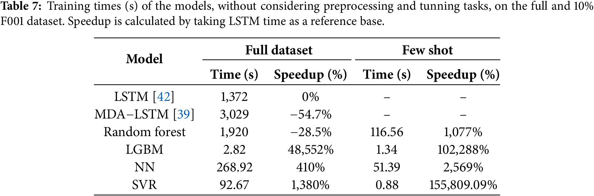
We used the training time of the LSTM model trained on the full dataset as a baseline to compute the percentage of increment or decrement in speedup. As can be observed, our proposal—SVR with embeddings—is strongly recommended not only for its accuracy (as seen in previous sections) but also for its low training times and therefore low power consumption.
Although the training times may seem low—requiring 50 min for the largest models—these figures only reflect the training of a single model configuration, noting the substantial differences that exist when using one or the other algorithm. In a real-world scenario, the training of a model typically involves cross-validation and hyperparameter tuning, which requires fitting many model configurations to find the best-performing one. As an example, the MDA-LSTM model has 10 configurable parameters. If only 2 possible values were considered for each parameter (the bare minimum to be considered configurable) and a 5-fold cross-validation was performed, this would result in training and evaluating 5120 models, which would take approximately 177 days using our setup, according to the measured times. In contrast, the same process using our SVR model in the few-shot scenario would only take around 1.25 h. Although more optimal tuning algorithms exist to prune unpromising parameter combinations, and more powerful hardware could accelerate the process, the difference in the training times remains remarkable. This difference not only affects the training time, but also the power consumption and, therefore, the energy costs and emissions.
We must also note that the time required for embedding creation is not included in the training times shown in Table 7. We consider this step part of the preprocessing, as it only needs to be performed once before the hyperparameter search. Moreover, generating embeddings for the entire training dataset takes 540 s, which means less than half the training time of the LSTM model. Therefore, even if we were to include this step as part of the training process, the SVR and NN models would still be the fastest.
Another important aspect in PdM problems is being able to react fast to the anomalies. That is why we measured the inference time of each model. To do it, we selected 1,000 observation windows and fed them to the models one at a time, computing the mean inference time and the standard deviation for each model. Table 8 presents both metrics in milliseconds (ms) for all models trained using the full training set and the reduced training set. As can be seen, all models, including DL models, have adequate times varying from a few ms to below one ms, which is fast enough for this dataset, where new data is recorded once every engine operating cycle.

All the experiments described in this paper were carried out using a PC equipped with an Intel Core i7-13700 K CPU, 32 GB of RAM, and an NVIDIA RTX A5000 GPU. All ML models were trained on the CPU, which has a maximum power consumption of 125 watts, whereas the DL ones were trained on the GPU, which has a maximum power consumption of 230 watts, 84% higher than the CPU. Thus, in addition to being much slower, DL models require more power-consuming hardware.
Regarding the estimation of the carbon impact, assuming a carbon efficiency of 0.432 kgCO2eq/kWh of our computer (value taken from the OECD’s 2014 yearly average), the full grid search training of the MDA-LSTM would emit a total of 422.08 kgCO2eq over a total of 4248 h of computation on the RTX A5000 GPU (TDP of 230W). In contrast, the training of the SVR model would emit 0.075 kgCO2eq over a total of 1.25 h of computation on the Intel Core i7-13700 K CPU (TDP of 125W). Estimations were conducted using the Machine Learning Emissions calculator1 presented in [60].
To recapitulate, this fourth experiment has demonstrated that using an ML model combined with the embedding generation strategy can significantly accelerate the training process. This advantage becomes even more evident when considering that tuning complex models typically requires extensive cross-validation and hyperparameter optimization. Simultaneously, the energy consumption and CO2 emissions associated with model training are lowered due to reduced computational demands and shorter training times.
The aim of this study has been to evaluate the use of TSFM for the RUL prediction on the CMAPSS dataset. We compare the performance of four ML models trained with embeddings generated by the Moment against both the same models trained with the original data and DL models chosen from recent literature. Next, we will answer the questions posed in Section 4.5 based on the results obtained in our benchmark.
The first question asked about the performance improvement achieved by ML techniques using embeddings. The experimentation shows that regarding RSME, this improvement is only achieved with models such as SVR on the most complex datasets, FD002 and FD004. However, it is not a beneficial strategy and may even degrade the performance of tree-based models, Random Forest and Gradient Boosting Machine, that are inherently capable of capturing non-linear relationships directly from the data. Regarding the score, models trained using the embeddings almost always obtain higher (worse) values, mainly due to the sensitivity of the formula to individual poor predictions.
Regarding the behavior of our proposal with respect to other models found in the literature, Table 4 shows that the ML models trained with embeddings offer competitive performance compared to simpler DL models and some hybrid models, especially in more complex data scenarios. However, hybrid attention-based DL models surpass the proposed models across all subsets, especially if a previous specific preprocessing is carried on (see row 16 and 22), albeit at the cost of longer training times and the need for larger datasets.
Another question asked whether models trained using the few-shot learning paradigm would achieve sufficient accuracy. This is where our proposal achieves the best results. Using embeddings improves the predictive performance of SVR and NN when training on a reduced training set, in our case using a 10% of the original training data. Notably, SVR achieves practically the same RMSE (less than a 4% of difference compared to using the full dataset) and outperforms simple DL models such as CNN and LSTM. Additionally, as demonstrated by the comparison using different dataset sizes, this effect becomes more noticeable as the size decreases.
Beyond performance benefits, the use of TSFM can be particularly valuable for organizations aiming to rapidly build and deploy ML models, as it eliminates the need for extensive manual feature engineering or dataset-specific preprocessing. By providing meaningful embeddings, TSFM simplifies the development pipeline, reduces dependency on domain expertise, and enables more scalable and generalizable solutions—aligning with the objectives of AutoML frameworks. This not only accelerates time-to-deployment but also facilitates experimentation across diverse applications with minimal adjustment [28], albeit at the cost of not always achieving the same level of predictive accuracy as highly specialized models.
Concerned with sustainability, we measure time and power consumption to train and use these models. ML models with TSFM embeddings significantly reduce training time compared to DL models while requiring less powerful hardware, and therefore, the pollutant emissions derived from the training are much lower. This is due to the lower complexity of the models and their ability to achieve competitive performance with fewer data samples.
In short, the combination of the Moment TSFM with classical models such as SVR creates a synergistic effect: Moment acts as a universal feature extractor, transforming multidimensional time series into latent representations that effectively preserve underlying degradation patterns. This enables simple models to focus on modelling the relationship between these embeddings and the RUL, eliminating the need for complex architectures or large volumes of labelled data. As a result, computational cost is significantly reduced without compromising predictive accuracy in low-labelled data scenarios. This approach circumvents the need to train DL models from scratch (e.g., LSTMs or transformers), which are often data- and resource-intensive. Instead, the embeddings generated by Moment leverage pre-trained knowledge in a zero-shot fashion and facilitate rapid adaptation to new contexts in few-shot learning setups, offering a practical and efficient solution for industrial scenarios with scarce labeled failure data.
Finally, a practitioner might reasonably consider that integrating the TSFM and the ML model into a unified training process could improve predictive accuracy. However, even though this could potentially yield better results, the limited amount of data in few-shot scenarios may not be enough to improve the performance of the TSFM. Moreover, given the complexity of TSFMs—with millions of parameters—the training process would require significantly more time and computational resources, making it more costly than most state-of-the-art models. This, indeed, would undermine the core motivation of our approach: to build lightweight, fast, and cost-effective predictive models by leveraging the representational power of TSFM without the burden of retraining them.
Limitations of the Study
The study presents certain limitations that should be noted. First, it focuses on the CMAPSS dataset, a synthetic benchmark for RUL prediction. While this synthetic dataset is widely used for comparing the performance of different algorithms in a controlled manner, this does not fully reflect the characteristics of a real environment where external factors influence the data, for example, generating random noise that can interfere in the model’s decision. Therefore, the results of this study may not be fully replicable in real scenarios, and experimentation with real-world datasets that present different common problems, such as strong noise, stationary features, or high proportions of missing data, should be performed.
One way to address this issue, while maintaining the FM-based approach, would be to fine-tune a large model using datasets that accurately capture the relevant characteristics of the problem (domain-aware adaptation), which, if not available, could be generated by means of data augmentation techniques. However, as this solution leads to more computational costs, as an initial step, we propose to experiment with other TSFMs for embedding generation when they are available.
It is also worth noting that the models were built using basic preprocessing techniques to maintain a general approach useful for any context, and to test the ability of FMs to absorb this task. However, the lack of this optimisation may reduce the accuracy of the proposed models.
Estimating the RUL remains an open challenge in predictive maintenance. Although several studies and surveys have been published in recent years addressing this issue from different approaches, the results are not definitive. It has been proven that the best predictors are achieved with hybrid DL models based on a combination of multidimensional attention layers and LSTMs. However, these models require long training times, large volumes of data, and expert knowledge for fine-tuning.
Both the versatility and effectiveness that FM have demonstrated in predictive and representational learning tasks [28] and the recent emergence of TSFM have led us to explore their applicability to RUL prediction. Our goal was to evaluate whether embeddings generated by TSFM are meaningful enough to enable the construction of competitive and simpler predictors with a reduced amount of training data and reduced preprocessing, thus lowering computational costs and processing time.
Our benchmark shows that training simple ML models, such as SVR or NN, with embeddings generated by Moment FM offers a viable alternative to complex DL models, particularly in few-shot scenarios where labeled data is scarce and computational resources are limited.
As future work, we plan to extend this experimentation to other artificial and real-world datasets and to explore the use of other FMs specifically designed for time series under a different architecture, such as TOTEM [35].
Acknowledgement: None.
Funding Statement: Funded by the Spanish Government and FEDER funds (AEI/FEDER, UE) under grant PID2021-124502OB-C42 (PRESECREL) and the predoctoral program “Concepción Arenal del Programa de Personal Investigador en formación Predoctoral” funded by Universidad de Cantabria and Cantabria’s Government (BOC 18-10-2021).
Author Contributions: Conceptualization, Ricardo Dintén and Marta Zorrilla; methodology, Marta Zorrilla; software, Ricardo Dintén; validation, Ricardo Dintén and Marta Zorrilla; investigation, Ricardo Dintén and Marta Zorrilla; resources, Ricardo Dintén and Marta Zorrilla; data curation, Ricardo Dintén; writing—original draft preparation, Ricardo Dintén; writing—review and editing, Marta Zorrilla; supervision, Marta Zorrilla; project administration, Marta Zorrilla; funding acquisition, Ricardo Dintén and Marta Zorrilla. All authors reviewed the results and approved the final version of the manuscript.
Availability of Data and Materials: The data that support the findings of this study are openly available in GitHub at [https://github.com/DintenR/TSFM_for_Few-shot_RUL_prediction (accessed on 2025 June 25)].
Ethics Approval: Not applicable.
Conflicts of Interest: The authors declare no conflicts of interest to report regarding the present study.
Abbreviations
| AI | Artificial Intelligence |
| AR | Auto-Regression |
| BERT | Bidirectional Encoder Representations from Transformers |
| CNN | Convolutional Neural Network |
| DL | Deep Learning |
| ELM | Extreme Learning Machine |
| IoT | Internet of Things |
| FSL | Few-shot Learning |
| GPT | Generative Pre-trained Transformer |
| GPU | Graphics Processing Unit |
| LGBM | Light Gradient Boosting Machine |
| LLM | Large Language Model |
| ML | Machine Learning |
| NPU | Neural Processing Unit |
| PdM | Predictive Maintenance |
| RF | Ramdom Forest |
| RCA | Root Cause Analysis |
| RNN | Recurrent Neural Network |
| RUL | Remaining Useful Life |
| SVR | Support Vector Regression |
| TPU | Tensor Processing Unit |
| TSFM | Time Series Foundation Models |
| VQVAE | Vector Quantized Variational Autoencoders |
Appendix A

Figure A1: Variables approaching failure with increasing trend
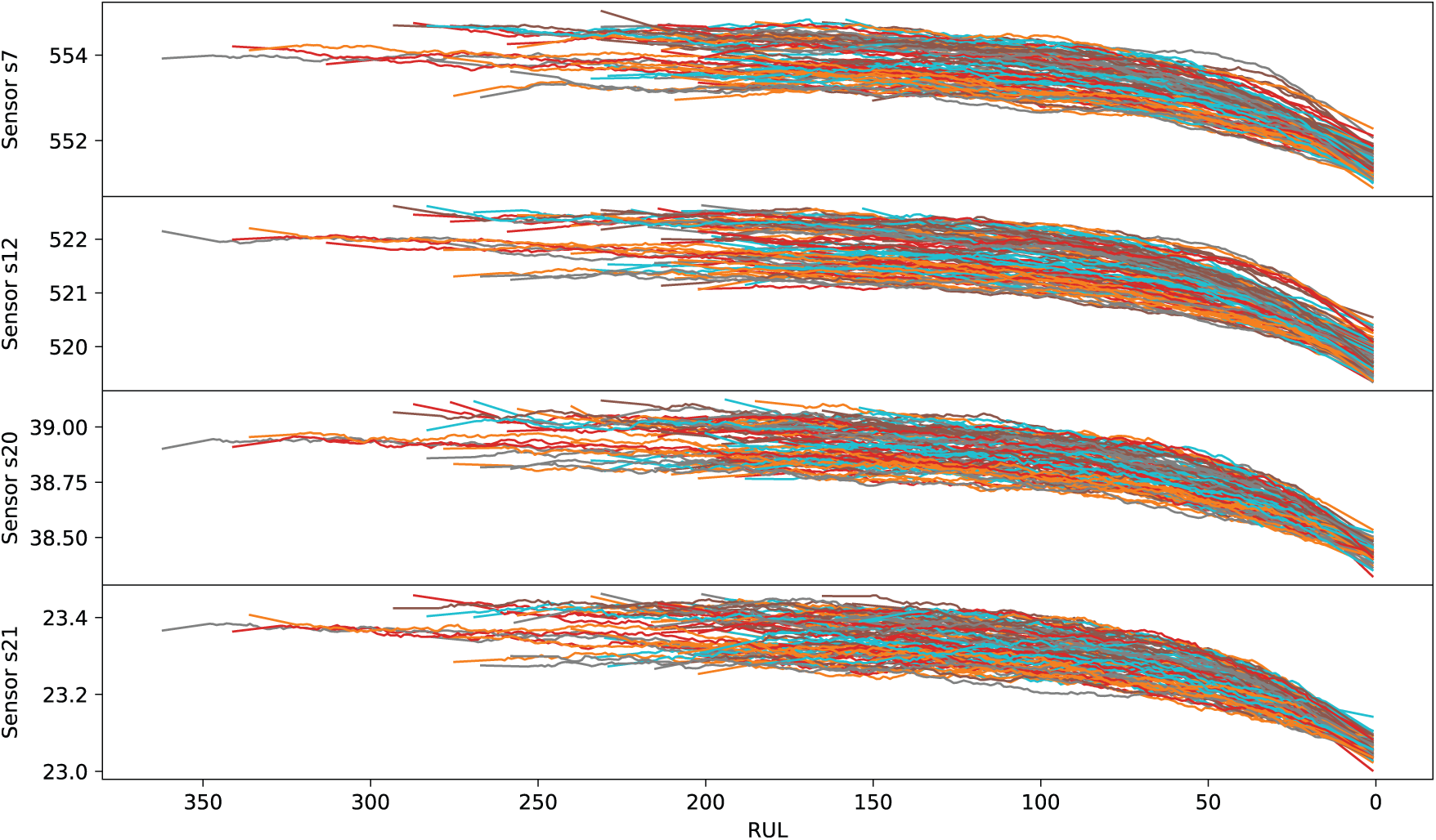
Figure A2: Variables approaching failure with decreasing trend

Figure A3: Variables approaching failure with random trend

Figure A4: Stationary variables approaching failure
Appendix B


1https://mlco2.github.io/impact#compute (accessed on 25 June 2025).
References
1. Keleko AT, Kamsu-Foguem B, Ngouna RH, Tongne A. Artificial intelligence and real-time predictive maintenance in industry 4.0: a bibliometric analysis. AI Ethics. 2022;4(2):553–77. doi:10.1007/s43681-021-00132-6. [Google Scholar] [CrossRef]
2. Serradilla O, Zugasti E, Rodriguez J, Zurutuza U. Deep learning models for predictive maintenance: a survey, comparison, challenges and prospects. Appl Intell. 2022;52(10):10934–64. doi:10.1007/s10489-021-03004-y. [Google Scholar] [CrossRef]
3. Wu F, Wu Q, Tan Y, Xu X. Remaining useful life prediction based on deep learning: a survey. Sensors. 2024;24(11):3454. doi:10.3390/s24113454. [Google Scholar] [PubMed] [CrossRef]
4. Wang X, Cui L, Wang H. Remaining useful life prediction of rolling element bearings based on hybrid drive of data and model. IEEE Sens J. 2022;22(17):16985–93. doi:10.1109/jsen.2022.3188646. [Google Scholar] [CrossRef]
5. Shyalika C, Wickramarachchi R, Sheth AP. A comprehensive survey on rare event prediction. ACM Comput Surv. 2024;57(3):70. doi:10.1145/3699955. [Google Scholar] [CrossRef]
6. Gao RX, Krger J, Merklein M, Mhring HC, Vncza J. Artificial intelligence in manufacturing: state of the art, perspectives, and future directions. CIRP Ann. 2024;73(2):723–49. doi:10.1016/j.cirp.2024.04.101. [Google Scholar] [CrossRef]
7. Zhang Q, Xu C, Li J, Sun Y, Bao J, Zhang D. LLM-TSFD: an industrial time series human-in-the-loop fault diagnosis method based on a large language model. Expert Syst Appl. 2025;264(4):125861. doi:10.1016/j.eswa.2024.125861. [Google Scholar] [CrossRef]
8. Cui L, Wang X, Wang H, Jiang H. Remaining useful life prediction of rolling element bearings based on simulated performance degradation dictionary. Mech Mach Theory. 2020;153(6):103967. doi:10.1016/j.mechmachtheory.2020.103967. [Google Scholar] [CrossRef]
9. Takayama R, Natsumeda M, Yairi T. A semi-supervised RUL prediction with likelihood-based pseudo labeling for suspension histories. In: 2023 IEEE International Conference on Prognostics and Health Management (ICPHM); 2023 Jun 5–7; Montreal, QC, Canada. p. 296–303. [Google Scholar]
10. Lin T, Song L, Cui L, Wang H. Advancing RUL prediction in mechanical systems: a hybrid deep learning approach utilizing non-full lifecycle data. Adv Eng Inform. 2024;61(6):102524. doi:10.1016/j.aei.2024.102524. [Google Scholar] [CrossRef]
11. Li S, Peng Y, Bin G, Shen Y, Guo Y, Li B, et al. Research on bearing fault diagnosis method based on CJBM with semi-supervised and imbalanced data. Nonlin Dyn. 2024;112(22):19759–81. doi:10.1007/s11071-024-10073-4. [Google Scholar] [CrossRef]
12. lv Y, Zhou N, Wen Z, Shen Z, Chen A. Remaining useful life prediction based on multisource domain transfer and unsupervised alignment. Eksploatacja I Niezawodnosc Maint Reliab. 2025;27(2):194116. doi:10.17531/ein/194116. [Google Scholar] [CrossRef]
13. Ding ZQ, Qin Q, Zhang YF, Lin YH. An uncertainty quantification and calibration framework for RUL prediction and accuracy improvement. IEEE Trans Instrum Meas. 2024;73(4):2535613. doi:10.1109/tim.2024.3485392. [Google Scholar] [CrossRef]
14. Zhang C, Gong D, Xue G. An uncertainty-incorporated active data diffusion learning framework for few-shot equipment RUL prediction. Reliab Eng Syst Saf 2025;254:110632. doi:10.1016/j.ress.2024.110632. [Google Scholar] [CrossRef]
15. Zhou T, Niu P, Wang X, Sun L, Jin R. One fits all: power general time series analysis by pretrained LM. arXiv:2302.11939. 2023. [Google Scholar]
16. Ren L, Wang H, Dong J, Jia Z, Li S, Wang Y, et. al. Industrial foundation model. IEEE Trans Cybern 2025;55(5):2286–301. doi:10.1109/TCYB.2025.3527632. [Google Scholar] [PubMed] [CrossRef]
17. Caspart R, Ziegler S, Weyrauch A, Obermaier H, Raffeiner S, Schuhmacher LP, et al. Precise energy consumption measurements of heterogeneous artificial intelligence workloads. In: Anzt H, Bienz A, Luszczek P, Baboulin M, editors. High performance computing. ISC high performance 2022 international workshops. Cham, Switzerland: Springer International Publishing; 2022. p. 108–21. doi:10.1007/978-3-031-23220-6_8. [Google Scholar] [CrossRef]
18. Li Z, He Q, Li J. A survey of deep learning-driven architecture for predictive maintenance. Eng Appl Artif Intell. 2024;133:108285. doi:10.1016/j.engappai.2024.108285. [Google Scholar] [CrossRef]
19. Li Z, Liu F, Yang W, Peng S, Zhou J. A survey of convolutional neural networks: analysis, applications, and prospects. IEEE Trans Neural Netw Learning Systems. 2020;33(12):6999–7019. doi:10.1109/tnnls.2021.3084827. [Google Scholar] [PubMed] [CrossRef]
20. Ucar A, Karakose M, Kirimça N. Artificial intelligence for predictive maintenance applications: key components, trustworthiness, and future trends. Appl Sci. 2024;14(2):898. doi:10.3390/app14020898. [Google Scholar] [CrossRef]
21. Li X, Yu D, Sren Byg V, Daniel Ioan S. The development of machine learning-based remaining useful life prediction for lithium-ion batteries. J Energy. 2023;82:103–21. doi:10.1016/j.jechem.2023.03.026. [Google Scholar] [CrossRef]
22. Tasci B, Omar A, Ayvaz S. Remaining useful lifetime prediction for predictive maintenance in manufacturing. Comput Ind Eng. 2023;184:109566. [Google Scholar]
23. Dintén R, Zorrilla M. Building and deployment of smart applications for anomaly detection and failure prediction in industrial use cases. Information. 2024;15(9):557. doi:10.3390/info15090557. [Google Scholar] [CrossRef]
24. Kim S, Seo YH, Park J. Transformer-based novel framework for remaining useful life prediction of lubricant in operational rolling bearings. Reliab Eng Syst Safety. 2024;251(2):110377. doi:10.1016/j.ress.2024.110377. [Google Scholar] [CrossRef]
25. Yu R, Chen M, Liu B. A triple-phase boost transformer for industrial equipment fault prediction. Neurocomputing. 2025;619(2):129137. doi:10.1016/j.neucom.2024.129137. [Google Scholar] [CrossRef]
26. Devlin J, Chang M, Lee K, Toutanova K. BERT: pre-training of deep bidirectional transformers for language understanding. arXiv:1810.04805. 2018. [Google Scholar]
27. Brown TB, Mann B, Ryder N, Subbiah M, Kaplan J, Dhariwal P, et al. Language models are few-shot learners. arXiv:2005.14165. 2020. [Google Scholar]
28. Liang Y, Wen H, Nie Y, Jiang Y, Jin M, Song D, et al. Foundation models for time series analysis: a tutorial and survey. In: Proceedings of the 30th ACM SIGKDD Conference on Knowledge Discovery and Data Mining. KDD ’24; 2024 Aug 25–29; Barcelona, Spain. 65556565 p. doi:10.1145/3637528.3671451. [Google Scholar] [CrossRef]
29. Jin M, Wang S, Ma L, Chu Z, Zhang JY, Shi X, et al. Time-LLM: time series forecasting by reprogramming large language models. In: The Twelfth International Conference on Learning Representations; 2024 May 7–11; Vienna, Austria. p. 1–24. [Google Scholar]
30. Liu C, Xu Q, Miao H, Yang S, Zhang L, Long C, et al. TimeCMA: towards LLM-empowered time series forecasting via cross-modality alignment. arXiv:2406.01638. 2024. [Google Scholar]
31. Xu Z, Bian Y, Zhong J, Wen X, Xu Q. Beyond trend and periodicity: guiding time series forecasting with textual cues. arXiv:2405.13522. 2024. [Google Scholar]
32. Xue H, Salim FD. PromptCast: a new prompt-based learning paradigm for time series forecasting. IEEE Trans Knowl Data Eng. 2024;36(11):6851–64. doi:10.1109/tkde.2023.3342137. [Google Scholar] [CrossRef]
33. Yu X, Chen Z, Ling Y, Dong S, Liu Z, Lu Y. Temporal data meets LLM – explainable financial time series forecasting. arXiv:2306.11025. 2023. [Google Scholar]
34. Goswami M, Szafer K, Choudhry A, Cai Y, Li S, Dubrawski A. MOMENT: a family of open time-series foundation models. arXiv:2402.03885. 2024. [Google Scholar]
35. Talukder SJ, Yue Y, Gkioxari G. TOTEM: TOkenized time series EMbeddings for general time series analysis. Transactions on machine learning research; 2024 [Internet]. [cited 2025 Jun 25]. Available from: https://openreview.net/forum?id=QlTLkH6xRC. [Google Scholar]
36. Bian Y, Ju X, Li J, Xu Z, Cheng D, Xu Q. Multi-patch prediction: adapting language models for time series representation learning. In: Proceedings of the 41st International Conference on Machine Learning. ICML’24; 2024 Jul 21-27; Vienna, Austria. [Google Scholar]
37. Chang C, Wang WY, Peng WC, Chen TF. LLM4TS: aligning pre-trained LLMs as data-efficient time-series forecasters. arXiv:2308.08469. 2024. [Google Scholar]
38. Vaswani A, Shazeer N, Parmar N, Uszkoreit J, Jones L, Gomez AN, et al. Attention is all you need. In: Guyon I, Luxburg UV, Bengio S, Wallach H, Fergus R, Vishwanathan S, et al., editors. Advances in neural information processing systems. Vol. 30. Red Hook, NY, USA: Curran Associates, Inc.; 2017. [Google Scholar]
39. Lai Z, Liu M, Pan Y, Chen D. Multi-dimensional self attention based approach for remaining useful life estimation. arXiv:2212.05772. 2022. [Google Scholar]
40. Elgeldawi E, Sayed A, Galal AR, Zaki AM. Hyperparameter tuning for machine learning algorithms used for arabic sentiment analysis. Informatics. 2021;8(4):79. doi:10.3390/informatics8040079. [Google Scholar] [CrossRef]
41. Hanifi S, Cammarono A, Zare-Behtash H. Advanced hyperparameter optimization of deep learning models for wind power prediction. Renew Energy. 2024;221(15):119700. doi:10.1016/j.renene.2023.119700. [Google Scholar] [CrossRef]
42. Zheng S, Ristovski K, Farahat A, Gupta C. Long Short-Term Memory Network for Remaining Useful Life estimation. In: 2017 IEEE International Conference on Prognostics and Health Management (ICPHM); 2017 Jun 19–21; Dallas, TX, USA. p. 88–95. [Google Scholar]
43. Asif O, Haider SA, Naqvi SR, Zaki JFW, Kwak KS, Islam SMR. A deep learning model for remaining useful life prediction of aircraft turbofan engine on C-MAPSS dataset. IEEE Access. 2022;10(1):95425–40. doi:10.1109/access.2022.3203406. [Google Scholar] [CrossRef]
44. Chen X, Jin G, Qiu S, Lu M, Yu D. Direct remaining useful life estimation based on random forest regression. In: 2020 global reliability and prognostics and health management (PHM-Shanghai); 2020 Oct 16–18; Shanghai, China. p. 1–7. doi:10.1109/phm-shanghai49105.2020.9281004. [Google Scholar] [CrossRef]
45. Sateesh Babu G, Zhao P, Li XL. Deep convolutional neural network based regression approach for estimation of remaining useful life. In: Navathe SB, Wu W, Shekhar S, Du X, Wang XS, Xiong H, editors. Database systems for advanced applications. Cham, Switzerland: Springer International Publishing. 2016. p. 214–28. doi:10.1007/978-3-319-32025-0_14. [Google Scholar] [CrossRef]
46. Wang J, Wen G, Yang S, Liu Y. Remaining useful life estimation in prognostics using deep bidirectional LSTM neural network. In: 2018 Prognostics Syst Health Management Conference (PHM-Chongqing); 2018 Oct 26–28; Chongqing, China. p. 1037–42. [Google Scholar]
47. Li J, Li X, He D. A directed acyclic graph network combined with CNN and LSTM for remaining useful life prediction. IEEE Access. 2019;7:75464–75. doi:10.1109/access.2019.2919566. [Google Scholar] [CrossRef]
48. Kong Z, Cui Y, Xia Z, Lv H. Convolution and long short-term memory hybrid deep neural networks for remaining useful life prognostics. Appl Sci. 2019;9(19):4156. doi:10.3390/app9194156. [Google Scholar] [CrossRef]
49. Mo H, Lucca F, Malacarne J, Iacca G. Multi-head CNN-LSTM with prediction error analysis for remaining useful life prediction. In: 2020 27th Conference of Open Innovations Association (FRUCT); 2020 Sep 7–9; Trento, Italy. p. 164–71. [Google Scholar]
50. Hong CW, Lee C, Lee K, Ko MS, Kim DE, Hur K. Remaining useful life prognosis for turbofan engine using explainable deep neural networks with dimensionality reduction. Sensors. 2020;20(22):6626. doi:10.3390/s20226626. [Google Scholar] [PubMed] [CrossRef]
51. Liu H, Liu Z, Jia W, Lin X. Remaining useful life prediction using a novel feature-attention-based end-to-end approach. IEEE Trans Ind Inf. 2021;17(2):1197–207. doi:10.1109/tii.2020.2983760. [Google Scholar] [CrossRef]
52. Peng C, Chen Y, Chen Q, Tang Z, Li L, Gui W. A remaining useful life prognosis of turbofan engine using temporal and spatial feature fusion. Sensors. 2021;21(2):418. doi:10.3390/s21020418. [Google Scholar] [PubMed] [CrossRef]
53. Amin U, Kumar K. Remaining useful life prediction of aircraft engines using hybrid model based on artificial intelligence techniques. In: 2021 IEEE International Conference on Prognostics and Health Management (ICPHM); 2021 Jun 7–9; Detroit, MI, USA. p. 1–10. [Google Scholar]
54. Yu K, Wang D, Li H. A prediction model for remaining useful life of turbofan engines by fusing broad learning system and temporal convolutional network. In: 2021 8th International Conference on Information, Cybernetics, and Computational Social Systems (ICCSS); 2021 Dec 10–12; Beijing, China. p. 137–42. [Google Scholar]
55. Liu Y, Zhang X, Guo W, Bian H, He Y, Liu Z. Prediction of remaining useful life of turbofan engine based on optimized model. In: 2021 IEEE 20th International Conference on Trust, Security and Privacy in Computing and Communications (TrustCom); 2021 Aug 18–20; Shenyang, China. p. 1473–7. [Google Scholar]
56. Chen X, Zeng M. Convolution-graph attention network with sensor embeddings for remaining useful life prediction of turbofan engines. IEEE Sens J. 2023;23(14):15786–94. doi:10.1109/jsen.2023.3279365. [Google Scholar] [CrossRef]
57. Keshun Y, Guangqi Q, Yingkui G. A 3-D attention-enhanced hybrid neural network for turbofan engine remaining life prediction using CNN and BiLSTM Models. IEEE Sens J. 2024;24(14):21893–905. doi:10.1109/jsen.2023.3296670. [Google Scholar] [CrossRef]
58. Liu Z, Zheng X, Xue A, Ge M, Jiang A. Multi-head self-attention-based fully convolutional network for RUL prediction of turbofan engines. Algorithms. 2024;17(8):321. doi:10.3390/a17080321. [Google Scholar] [CrossRef]
59. Hua J, Zhang Y, Zhang D, He J, Wang J, Fang X. Dynamic feature-aware graph convolutional network with multisensor for remaining useful life prediction of turbofan engines. IEEE Sens J. 2024;24(18):29414–28. doi:10.1109/jsen.2024.3435071. [Google Scholar] [CrossRef]
60. Lacoste A, Luccioni A, Schmidt V, Dandres T. Quantifying the carbon emissions of machine learning. arXiv:1910.09700. 2019. [Google Scholar]
Cite This Article
 Copyright © 2025 The Author(s). Published by Tech Science Press.
This work is licensed under a Creative Commons Attribution 4.0 International License , which permits unrestricted use, distribution, and reproduction in any medium, provided the original work is properly cited.
 Downloads
 Citation Tools