3D Exact Magneto-Electro-Elastic Static Analysis of Multilayered Plates

1  Introduction

Magneto-Electric (ME) coupling in magnetostrictive-piezoelectric multiferroic structures consent to induce an electric field in the structure due to an applied magnetic field, and on the contrary, a magnetic response consequent to an applied electric field. ME voltage coefficient (the ratio of an induced electric field to an applied magnetic field) is the key parameter to measure ME coupling strength [1–3]. In the case of smart structures (both sensor and actuator configurations), this coupling evaluation is fundamental and for this reason 1D, 2D and 3D numerical/analytical magneto-electro-elastic models have great importance in such investigations.

In the field of 1D models, generally applied to structures where one dimension is predominant with respect to the other two dimensions in the cross-section, several approaches have been proposed in recent years. Milazzo and Orlando [4] developed an elastic equivalent single layer finite element formulation for shear deformable and straight magneto-electro-elastic (MEE) laminated beam. The generalized exp-function method was employed in [5] to investigate the families of solitary wave solutions of one-dimensional nonlinear longitudinal wave equations in a MEE circular rod. In [6], an MEE functionally graded Timoshenko microbeam model was developed thanks to both the use of the variational formulation and the extended modified couple stress theory proposed to understand microstructure effects. Plane-strain equations for static deformations of anisotropic layered MEE cylinders were solved in [7] by assuming layers as perfectly bonded at the interfaces and by solving these equations thanks to the separation of variables and eigenfunction expansion. Huang et al. [8] showed both analytical and semi-analytical solutions for anisotropic functionally graded MEE beams under an arbitrary load. The generalized plane stress problem took into account stress functions, electric displacement, and magnetic induction functions.

2D models can be applied in the numerical or analytical form to plates and shells, which are structures where the two dimensions in the in-plane directions are predominant with respect to the dimension through the thickness direction. Chen et al. [9] proposed the state-vector approach to analyze free vibrations of MEE laminated plates, where extended displacements and stresses are split up into in-plane and out-of-plane variables. Phoenix et al. [10] adopted Reissner’s mixed variational theorem for static and dynamic analyses of coupled MEE problems in the case of composite/piezoelectric plates. A coupled finite element method was proposed in [11] considering higher-order approximate interpolation displacement, electric potential and magnetic potential shape functions. A fully geometrically nonlinear finite rotation shell element based on Reissner–Mindlin first-order shear deformation theory was proposed by Rao et al. in [12] for static analysis of layered MEE structures. Wang et al. [13] developed an hygrothermo-magneto-electro-elastic coupled and improved enriched finite element formulation to analyze functionally graded MEE structures; quadrilateral elements were used in this study. Carrera et al. [14,15] proposed refined 2D finite elements for MEE plates based on the principle of virtual displacements and on the Reissner’s mixed variational theorem, respectively. A closed form solution for MEE bending of rectangular thin plates was developed in [16] using the Kirchhoff thin-plate theory. The large deflection of MEE laminated plates was investigated by Milazzo [17], where the first-order shear deformation theory and the von Karman stress function approach were employed. Alaimo et al. [18,19] developed an isoparametric four-node finite element for multilayered MEE plates, the first order shear deformation theory was employed. Quasi-static behavior investigations were proposed, and then large deflections in MEE multilayered plates were also analyzed. Analytical solutions for general static deformations of spherically anisotropic and multilayered MEE hollow spheres were proposed in [20]. A partial mixed layerwise finite element model for adaptive plate structures was formulated in [21] using transverse stresses, displacement components, electric and magnetic potentials as primary variables. Explicit solutions for Navier’s and Lévy’s solutions were derived in [22] for unsymmetric MEE composite laminated thin plates. The scaled boundary finite element method was employed in [23] to study the deformation of a MEE plate. The inhomogeneous MEE coupling element-free Galerkin method, showed in [24] by Zhou et al. was used for solving static behaviors of structures where different temperature fields were simulated. A multiphysics plate model for the analysis of MEE composite laminates was shown in [25] by applying the variational asymptotic method, reducing the multiphysically coupled three-dimensional model to a series of two-dimensional plate models. A higher-order thickness-stretched model was proposed in [26] for the electro-elastic analysis of the composite graphene origami-reinforced square plate sandwiched by piezoelectric/piezomagnetic layers subjected to multifield loads (thermal, electric, magnetic and mechanical). Kiarasi et al. [27] investigated the hygrothermal effect on natural frequencies for functionally graded annular plates integrated with piezo-magneto-electro-elastic layers resting on Pasternak foundations. The effects of hygro-thermal environments on smart composite nanoplates were investigated in [28,29] using coupled MEE constitutive and governing equations solved via a strain gradient nonlocal theory and analytical methods. The magneto-electric effect on waves in functionally graded piezoelectric-piezomagnetic fan-shaped cylindrical structures was explored in [30] using the double Legendre orthogonal polynomial method and the Heaviside function. The nonlocal static analysis using Reddy’s high-order shear deformation theory of MEE sandwich micro/nano-plates with functionally graded carbon nanotube core in a hygrothermal environment was studied in [31]. Zhang et al. [32] proposed the scaled boundary finite element method incorporated with the precise integration technique for static and free vibration of multilayered MEE plates. The multi-physics zonal Galerkin free element method was proposed in [33] for static and transient responses of functionally graded MEE structures. The MEE-coupled isogeometric analysis was shown in [34] to understand the behaviour of structures thanks to the use of Non-Uniform Rational B-Spine functions. Tornabene et al. [35,36] proposed refined 2D generalized differential quadrature methods for the thermo-hygro-electro-magneto-elastic analysis of double-curved shells using an equivalent layerwise approach. Ren et al. [37] investigated static magneto-electro-hygro-elastic multi-field coupling problems using a stabilized node-based smoothed radial point interpolation method. Under the assumption of quasi-static electric and magnetic fields, the MEE analysis including the medium and its environment was proposed in [38].

3D analytical/numerical models for the electro-magneto-elastic analysis of multilayered structures are less numerous than 2D models. They can be applied to thick and anisotropic multilayered structures to obtain correct evaluations of elastic, magnetic and electric variables through the thickness direction. The study of isotropic functionally graded MEE circular plate behavior under uniform load was considered in [39]. The analytical solution for a three-dimensional transversely isotropic axisymmetric multilayered MEE circular plate under simply supported boundary conditions was proposed in [40]. In [41], the coupled governing equations for MEE plates were derived and solved via the COMSOL software considering a three-dimensional finite element approach. Pan [42] derived an exact three-dimensional model for anisotropic MEE simply supported multilayered plates under static loads. Derivation of the state vector equations for the three dimensional MEE orthotropic media was presented by Wang et al. in [43] from governing equations and then they were employed for the analysis of multilayered MEE plates. The static response of MEE plates subjected to hygrothermal loads was investigated in [44] using the finite element method derived from the principle of total potential energy. Pan and Heyliger [45] derived analytical solutions for free vibrations of three-dimensional MEE anisotropic multilayered plates under simply supported boundary conditions. A modified Pagano method was developed in [46] for the three-dimensional analysis of functionally graded simply supported rectangular plates subjected to magneto-electro-mechanical loads. The static behavior of doubly curved functionally graded MEE shells under mechanical loads, electric displacements and magnetic fluxes was investigated in [47] via the asymptotic approach.

The 3D exact and coupled electro-magneto-elastic plate model in this study tries to fill the gap of a few works on 3D models in the literature. The governing equations in 3D form are completely coupled and they are solved in in-plane directions using Navier-type solutions and through the thickness utilizing the exponential matrix method. The multilayered approach is layerwise, and equilibrium and compatibility conditions are fully satisfied at each layer interface. The same authors proposed a similar 3D coupled electro-elastic model in [48] and a similar 3D coupled magneto-elastic model in [49]; the first original work for the pure elastic analysis was given in [50]. This study fully couples elastic, magnetic, and electric fields for the first time using the exponential matrix method and the layerwise approach. It proposes several static analyses for multilayered plates in sensor and actuator configurations. Governing, constitutive, and geometrical relations are discussed in Section 2, the solution procedure is developed in Section 3, results (both preliminary assessments and new benchmarks) are discussed in Section 4, and finally, the main conclusions are presented in Section 5.

2  Coupled Magneto-Electro-Elastic 3D Plate Model

This section presents equations for the 3D coupled magneto-electro-elastic plate problem. Each subsection is devoted to equations involved in the present formulation. In the first one, constitutive and geometrical relations are given. In the second one, the 3D equilibrium equations, the 3D divergence equation for the magnetic induction and the 3D divergence equation for the electric displacement are shown for the plate case. The geometry of the plate considered in this study is shown in Fig. 1.

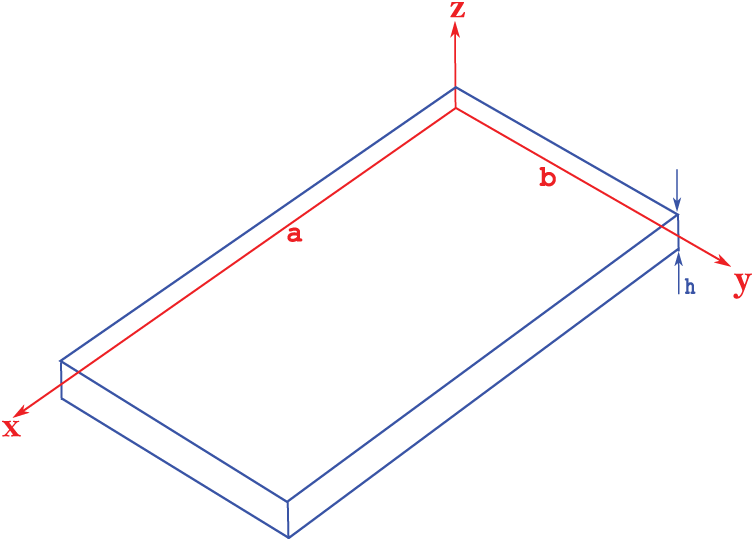
Figure 1: Geometry of the plate

2.1 Constitutive and Geometrical Relations

Constitutive and geometrical relations are utilized to couple magnetic, electric and elastic fields. For the present 3D coupled magneto-electro-elastic problem, constitutive equations can be written in the orthogonal structural reference system (x, y, z) for plates embedding k layers:

σk=Ckεk−ekTEk−qkTHk,(1a)

Dk=ekεk+εkEk+dkHk,(1b)

Bk=qkεk+dkEk+μkHk.(1c)

σk is the 6×1 stress vector, Ck is the 6×6 elastic coefficient matrix, εk is the 6×1 strain vector, ek is the 3×6 piezoelectric coefficient matrix, Ek is the 3×1 electric field vector, qk is the 3×6 piezomagnetic coefficient matrix, Hk is the 3×1 magnetic field vector, Dk is the 3×1 electric displacement vector, εk is the 3×3 electric permittivity matrix, dk is the 3×3 electro-magnetic coupling coefficient matrix, Bk is the 3×1 magnetic induction vector and μk is the 3×3 magnetic permittivity matrix. T means the transpose of a vector or a matrix.

All vectors and matrices involved in Eq. (1) are here explicitly written:

σk={σxxkσyykσzzkσyzkσxzkσxyk},Ck=[C11kC12kC13k00C16kC12kC22kC23k00C26kC13kC23kC33k00C36k000C44kC45k0000C45kC55k0C16kC26kC36k00C66k],εk={εxxkεyykεzzkγyzkγxzkγxyk},(2a)

ek=[000e14ke15k0000e24ke25k0e31ke32ke33k00e36k],Ek={ℰxkℰykℰzk},qk=[000q14kq15k0000q24kq25k0q31kq32kq33k00q36k],(2b)

Hk={ℋxkℋykℋzk},Dk={𝒟xk𝒟yk𝒟zk},εk=[ε11kε12k0ε12kε22k000ε33k],dk=[d11kd12k0d12kd22k000d33k],(2c)

Bk={ℬxkℬykℬzk},μk=[μ11kμ12k0μ12kμ22k000μ33k].(2d)

Geometrical relations for plates can be written as:

εk=Δuk,(3a)

Hk=−ΔHψk,(3b)

Ek=−ΔEϕk,(3c)

where Δ is the 6×3 derivative matrix for the elastic field, ΔH is the 3×1 derivative vector for the magnetic field and ΔE is the 3×1 derivative vector for the electric field. These derivative matrices and vectors are expressed as:

Δ=[∂∂x000∂∂y000∂∂z0∂∂z∂∂y∂∂z0∂∂x∂∂y∂∂x0],ΔH=ΔE=[∂∂x∂∂y∂∂z].(4)

∂∂x, ∂∂y and ∂∂z indicate partial derivatives in x, y and z directions, respectively.

2.2 3D Magneto-Electro-Elastic Governing Equations for Plates

Governing equations for plates include the three 3D equilibrium equations for the elastic field, the 3D divergence equation of the magnetic induction for the magnetic field and the 3D divergence equation of the electric displacement for the electric field. These five equations are coupled in a unique system.

The three 3D equilibrium equations for the plate case written in terms of stresses are:

σxx,xk+σxy,yk+σxz,zk=0,(5a)

σxy,xk+σyy,yk+σyz,zk=0,(5b)

σxz,xk+σyz,yk+σzz,zk=0,(5c)

where stresses σxxk,σxyk,σxzk,σxyk,σyyk,σβzk,σzzk are dependent from x, y and z. For this reason, the present formulation has a three-dimensional approach.

The 3D divergence equation of the magnetic induction for plates can be written as:

ℬx,xk+ℬy,yk+ℬzk,z=0.(6)

Analogously, the 3D divergence equation of the electric displacement for plates is:

𝒟x,xk+𝒟y,yk+𝒟zk,z=0.(7)

Subscripts, x, y and, z indicate partial derivatives with respect to x, y and z directions, respectively.

3  Navier Harmonic Forms and Exponential Matrix Method

The set of equations for the 3D magneto-electro-elastic problem for plates is composed of Eqs. (5)–(7). The resolution method is proposed and discussed in depth.

In order to write the five second-order differential equations in terms of primary variables, geometric and constitutive relations (Eqs. (1) and (3)) have to be introduced into Eqs. (5)–(7). In this way, the 3D governing equations are written in terms of primary variables uk, vk, wk, ψk and ϕk. In addition, the following terms must be set at zero to have a closed from solution:

C16k=C26k=C36k=C45k=0,e14k=e25k=e36k=0,q14k=q25k=q36k=0,ε12k=0,μ12k=0,d12k=0.(8)

In order to solve the 3D magneto-electro-elastic problem for plates, the first step is the imposition of the Navier harmonic forms in the in-plane directions x and y. These harmonic forms, in the case of simply supported sides, can be explicitly written as:

uk(x,y,z)=Uk(z)cos⁡(α¯x)sin⁡(β¯y),(9a)

vk(x,y,z)=Vk(z)sin⁡(α¯x)cos⁡(β¯y),(9b)

wk(x,y,z)=Wk(z)sin⁡(α¯x)sin⁡(β¯y),(9c)

ϕk(x,y,z)=Φk(z)sin⁡(α¯x)sin⁡(β¯y),(9d)

ψk(x,y,z)=Ψk(z)sin⁡(α¯x)sin⁡(β¯y),(9e)

where Uk(z),Vk(z),Wk(z),Φk(z),Ψk(z) are the amplitudes for each primary variable. Terms α¯ and β¯ are written as:

α¯=mπa,β¯=nπb,(10)

considering m, n the half-wave numbers and a, b the in-plane dimensions of the plate in x and y directions, respectively.

Navier harmonic forms fulfill the boundary conditions for the simply-supported constraints:

ϕk=0,     ψk=0,     wk=0,     vk=0,     σxxk=0,     for     x=0,a,ϕk=0,     ψk=0,     wk=0,     uk=0,     σyyk=0,     for     y=0,b.(11)

The imposition of harmonic forms of Eq. (9) permits to get the 3D magneto-electro-elastic set of equations in terms of primary variable amplitudes:

(−α¯2C11k−β¯2C66k)Uk+(−α¯β¯C12k−α¯β¯C66k)Vk+(α¯C13k+α¯C55k)W,zk+C55kU,zzk++(α¯e31k+α¯e15k)Φ,zk+(α¯q31k+α¯q15k)Ψ,zk=0,(12a)

(−α¯2C66k−β¯2C22k)Vk+(−α¯β¯C12k−α¯β¯C66k)Uk+(β¯C44k+β¯C23k)Wzk+C44kV,zzk++(β¯e32k+β¯e24k)Φ,zk+(β¯q32k+β¯q24k)Ψ,zk=0,(12b)

(−α¯2C55k−β¯2C44k)Wk+(−α¯C55k−α¯C13k)U,zk+(−β¯C44k−β¯C23k)V,zk+C33kW,zzk++(−α¯2e15k−β¯2e24k)Φk+(−α¯2q15k−β¯2q24k)Ψk+e33kΦ,zzk+q33kΨ,zzk=0,(12c)

(−α¯2e15k−β¯2e24k)Wk+(−α¯e15k−α¯e31k)U,zk+(−β¯e24k−β¯e32k)V,zk+e33kWzzk++(α¯2ε11k+β¯2ε22k)Φk−ε33kΦ,zzk+(α¯2d11k+β¯2d22k)Ψk−d33kΨ,zzk=0,(12d)

+(−α¯2q15k−β¯2q24k)Wk+(−α¯q15k−α¯q31k)U,zk+(−β¯q24k−β¯q32k)V,zk+q33kWzzk++(α¯2d11k+β¯2d22k)Φk−d33kΦ,zzk+(α¯2μ11k+β¯2μ22k)Ψk−μ33kΨ,zzk=0.(12e)

The exponential matrix method is the approach adopted to solve Eq. (12) along the thickness direction. To get first order differential equations in z starting from the second order differential equations (Eq. (12)), a redoubling procedure must be done. This procedure also duplicates the number of unknowns: Uk(z), Vk(z), Wk(z), Φk(z), Ψk(z), U,zk(z), V,zk(z), W,zk(z), Φ,zk(z), Ψ,zk(z). The use of the exponential matrix resolution method allows correct calculations of first derivatives in z because they are now the primary variables of the problem. In this way, the computation of stresses, strains, electric displacement, and magnetic induction along thickness direction is always correct and in three-dimensional form.

Eq. (12) can be written in a compact matrix form as follows:

DkX,zk=AkXk⇒X,zk=A∗kXk,(13)

where Dk and Ak are 10×10 matrices, X,zk is the 10×1 vector of unknowns derived in z, Xk is the 10×1 vector of unknowns and A∗k=D−1kAk is a 10×10 matrix. Vector of unknowns Xk is defined as follows:

Xk={Uk,Vk,Wk,Φk,Ψk,U,zk,V,zk,W,zk,Φ,zk,Ψ,zk}T.(14)

A possible solution of Eq. (13) can be obtained with the exponential matrix method as follows:

Xk(hk)=exp(A∗khk)Xk(0)=[∑i=0N(A∗k)ii!hki]Xk(0),(15)

where (A∗k)0=I is the 10×10 identity matrix, and hk is the thickness of each k layer. The exponential matrix in Eq. (15) is computed considering the Taylor expansion.

The imposition of the interlaminar continuity between two adjacent k layers permits the layerwise approach. So, these conditions need to be imposed on primary variables, transverse shear stresses, transverse normal stresses, transverse normal electric displacement and transverse normal magnetic induction:

ubk=utk−1,     vbk=vtk−1,     wbk=wtk−1,     ϕbk=ϕtk−1,     ψbk=ψtk−1,(16a)

σxzbk=σxztk−1,     σyzbk=σyztk−1,     σzzbk=σzztk−1,     𝒟zbk=𝒟ztk−1,     ℬzbk=ℬztk−1.(16b)

t is the top of the previous k−1 layer, and b is the bottom of the adjacent k layer. k goes from 1 to NL (total number of layers). Introducing Eq. (9) in Eq. (16), interlaminar continuity conditions are:

Ubk=Utk−1,(17a)

Vbk=Vtk−1,(17b)

Wbk=Wtk−1,(17c)

Φbk=Φtk−1,(17d)

Ψbk=Ψtk−1,(17e)

C55kα¯Wbk+C55kU,zbk+e15kα¯Φbk+q15kα¯Ψbk=C55k−1α¯Wtk−1+C55k−1U,ztk−1+e15k−1α¯Φtk−1+q15k−1α¯Ψtk−1,(17f)

C44kβ¯Wbk+C44kV,zbk+e24kβ¯Φbk+q24kβ¯Ψbk=C44k−1β¯Wtk−1+C44k−1V,ztk−1+e25k−1β¯Φtk−1+q25k−1β¯Ψtk−1,(17g)

C13kα¯Ubk−C23kβ¯Vbk+C33kW,zbk+e33kΦ,zbk+q33kΨ,zbk=−C13k−1α¯Utk−1−C23k−1β¯Vtk−1+C33k−1W,ztk−1++e33k−1Φ,ztk−1+q33k−1Ψ,ztk−1,(17h)

−e31kα¯Ubk−e32kβ¯Vbk+e33kW,zbk−ε33kΦ,zbk−d33kΨ,zbk=−e31k−1α¯Utk−e32k−1β¯Vtk+e33k−1W,ztk−1+−ε33k−1Φ,ztk−1−d33k−1Ψ,ztk−1,(17i)

−q31kα¯Ubk−q32kβ¯Vbk+q33kW,zbk−d33kΦ,zbk−μ33kΨ,zbk=−q31k−1α¯Utk−q32k−1β¯Vtk+q33k−1W,ztk−1+−d33k−1Φ,ztk−1−μ33k−1Φ,ztk−1.(17j)

All these equations can be compacted in a matrix form as follows:

Xbk=Tk,k−1Xtk−1,(18)

where Tk,k−1 is the 10×10 transfer matrix between layer k and layer k−1. Terms of matrix Tk,k−1 include constant coefficients coming from a rearrangement of Eq. (17) in terms of primary variables.

Therefore, the solution along the z direction is possible by considering a recursive substitution as follows:

XNL(hNL)=A∗∗NLTNL,NL−1…T2,1A∗∗1X1(0)⇒XNL(hNL)=HmX1(0),(19)

where Hm is the 10×10 matrix; its terms consider plate dimensions, thickness and material layer configuration of the multilayered plate. The matrix Hm is always a 10×10 matrix, despite the number of layers along the thickness direction and the orderN of the exponential matrix.

Load boundary conditions can be imposed on the external surfaces of the plate in terms of mechanical loads, electric potential, and/or magnetic potential. The transverse normal mechanical load has the following harmonic form:

pzk(x,y,z)=Pzk(z)sin⁡(α¯x)sin⁡(β¯y),(20)

harmonic forms of electric potential and magnetic potential are already described in Eqs. (9d) and (9e), respectively. Pzk(z), Φk(z) and Ψk(z) are the amplitudes of external mechanical, electric, and magnetic loads. They can be imposed at the bottom (b) of the first layer (k=1) or at the top (t) of the last layer (k=NL).

Load boundary conditions can be written in matrix form as:

[B1b1B2b1B3b10000B4b1B5b1B6b10B7b1B8b1B9b1B10b10B11b1000B12b10B13b1B14b1B15b1B16b1000000010000000000100000]{Ub1Vb1Wb1Φb1Ψb1U,z1bV,z1bW,z1bΦ,z1bΨ,z1b}={Pzb100Φb1Ψb1}forz=−h/2,(21)

[B1tNLB2tNLB3tNL0000B4tNLB5tNLB6tNL0B7tNLB8tNLB9tNLB10tNL0B11tNL000B12tNL0B13tNLB14tNLB15tNLB16tNL000000010000000000100000]{UtNLVtNLWtNLΦtNLΨtNLU,ztNLV,ztNLW,ztNLΦ,ztNLΨ,ztNL}={PztNL00ΦtNLΨtNL}forz=+h/2,(22)

that can be further compacted in the following form:

Bb1Xb1=Pb1,(23a)

BtNLXtNL=PtNL,(23b)

where Bb1 and BtNL are the 5×10 load boundary condition matrix and Pb1 and PtNL are the 5×1 bottom and top load vectors of the plate, respectively. Considering Eq. (19), it is possible to write Eq. (23) as:

[Bb1BtNLHm]Xb1={Pb1PtNL}⇒EXb1=P,(24)

where E is the 10×10 matrix including the multilayered configuration characteristics.

The present 3D magneto-electro-elastic formulation can analyze both sensor and actuator configurations. The vector of external loads P assumes a slightly different form in the two cases:

P={Pzb10000PztNL0000}for the sensor case,(25)

P={000Φb1Ψb1000ΦtNLΨtNL}for the actuator case.(26)

Due to the resolution of the linear system proposed in Eq. (24) and considering the recursive use of Eqs. (15) and (18), trends of primary variables along the thickness direction can be evaluated. The presented analytical formulation is simple and elegant, permitting the correct results for each thickness ratio of the plate. Matlab code (done with Matlab R2022a version) runs analysis in a few seconds, as the heavier computation cost regards iterative matrix multiplications of 10×10 matrices.

4  Results

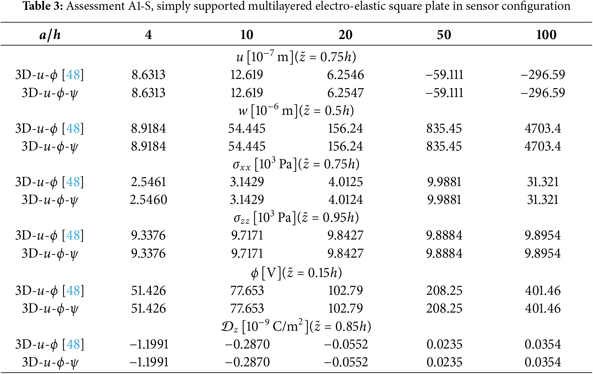
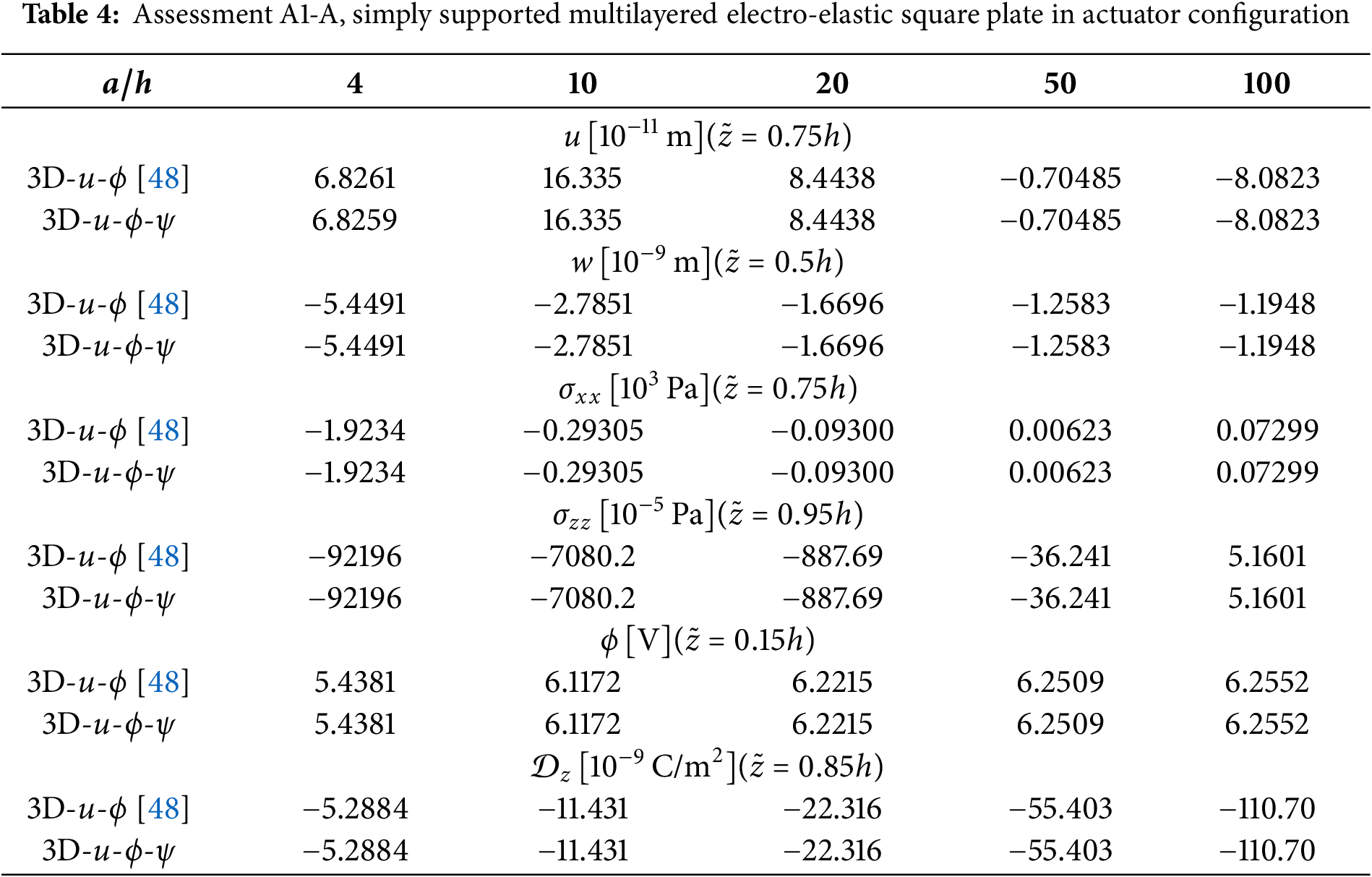
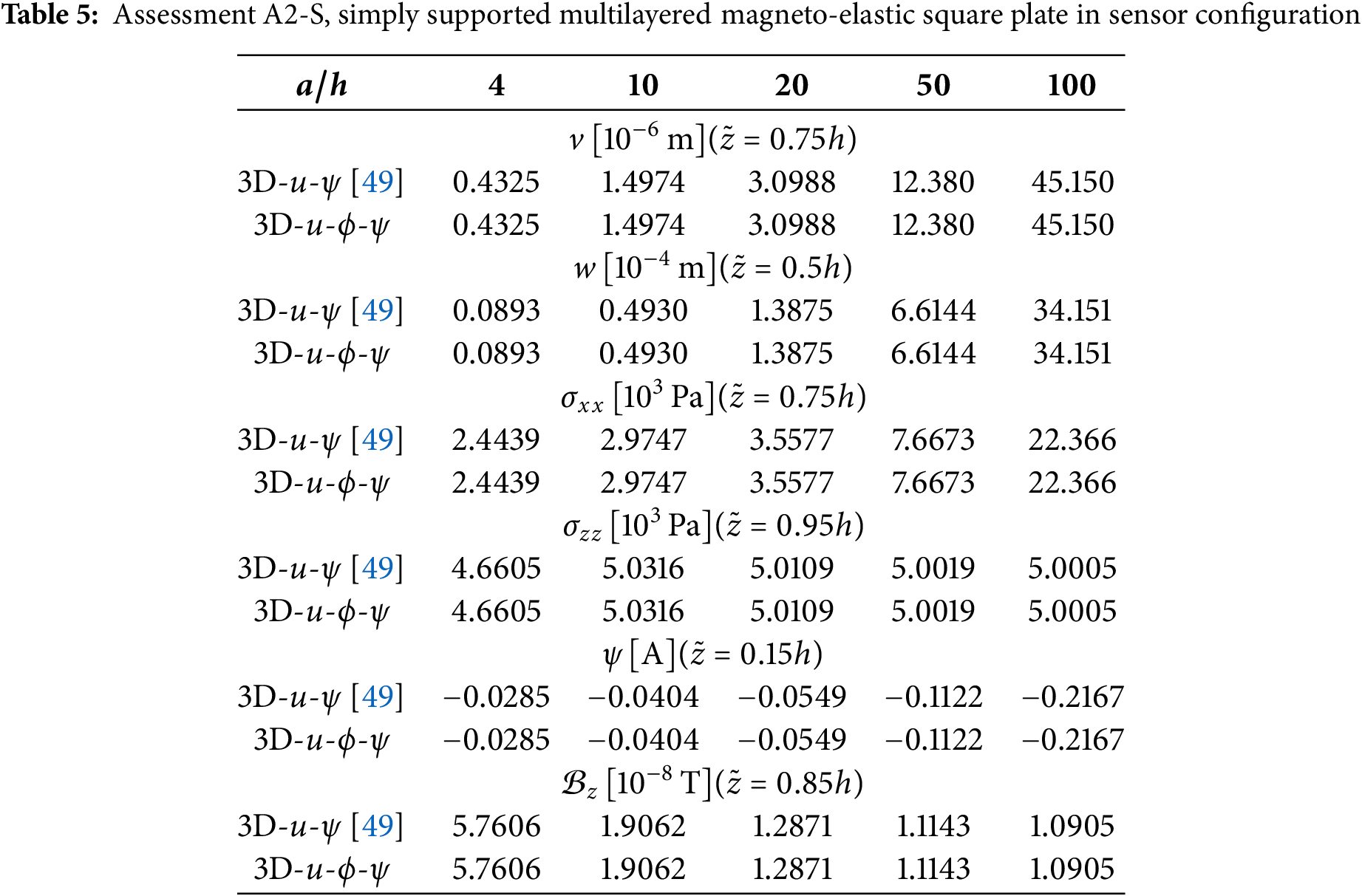
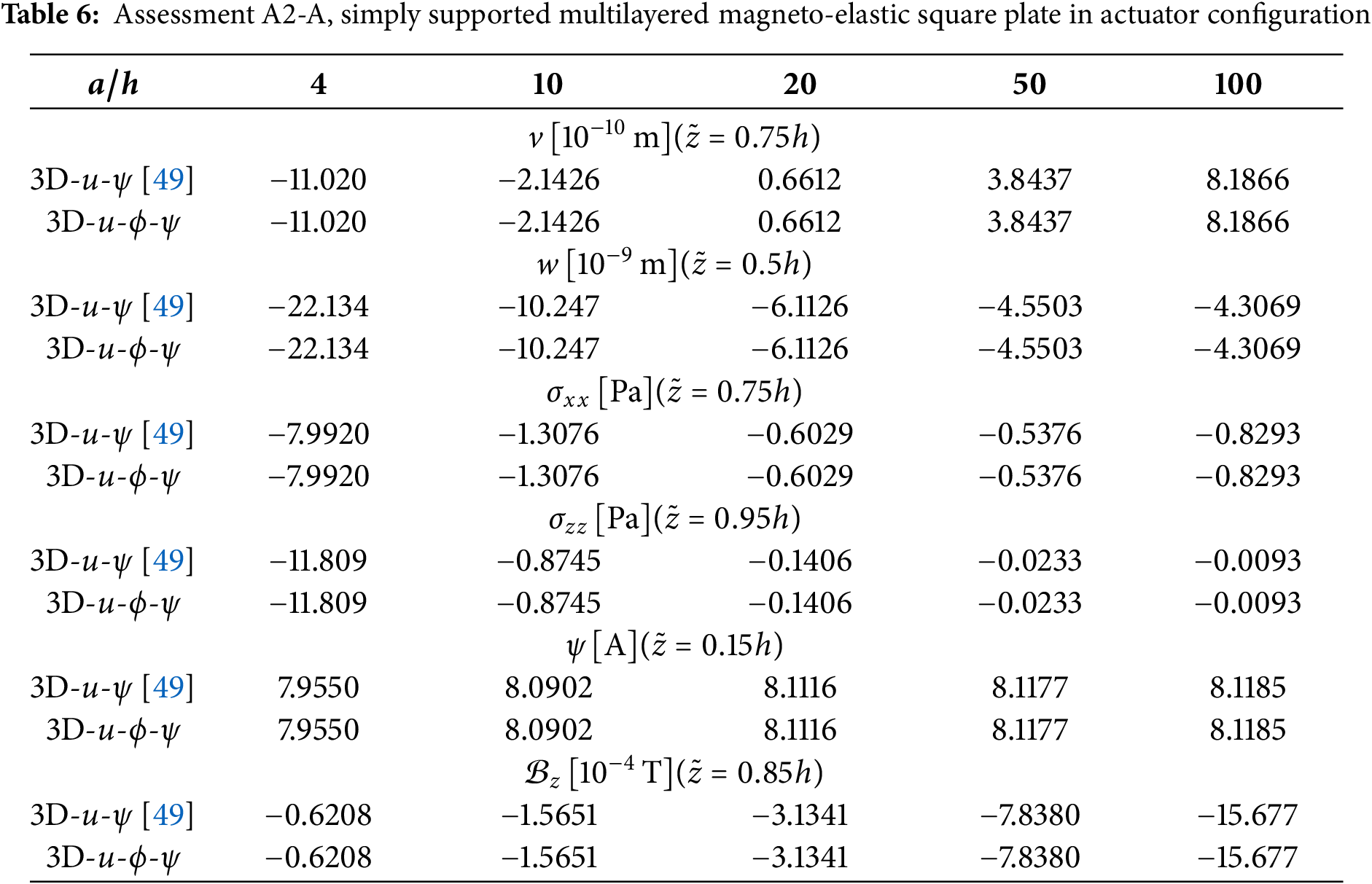
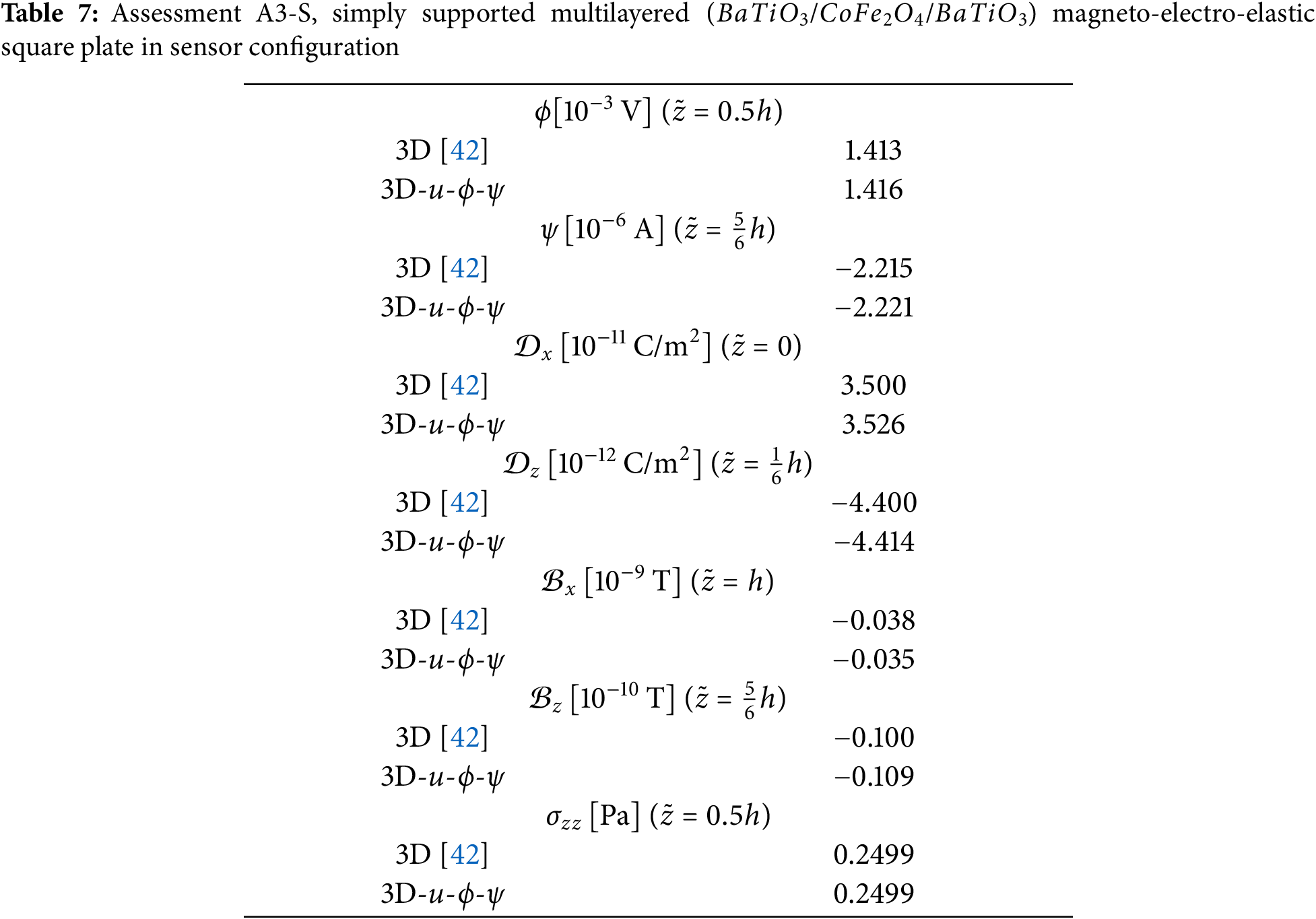
The present section is divided into an assessment subsection and a new benchmark subsection. In the assessment subsection, the present magneto-electro-elastic 3D-u-ϕ-ψ model is compared to the 3D electro-elastic (3D-u-ϕ) model developed in [48], with the 3D magneto-elastic (3D-u-ψ) model developed in [49] and with the 3D magneto-electro-elastic model developed by Pan [42]. The acronym 3D-u-ϕ-ψ summarizes the main peculiarities of the model: three-dimensional formulation where primary variables are displacements and their derivatives in z (stated as u), electric potential and its derivative in z (indicated with ϕ) and magnetic potential and its derivative in z (indicated with ψ). In the benchmark subsection, a new multilayered square plate in both sensor and actuator configurations is proposed considering different a/h thickness ratios (from thick to thin plates). As far as the authors know, magnetic permittivity coefficients μ1 and μ2 can be found in literature mainly with the negative sign (μ1=μ2=−590103 nH/m), as assessed and validated in [51], but also with a positive sign (μ1=μ2=590103 nH/m) [52]. For this time, the proposed benchmark case is provided considering μ1 and μ2 with both signs to overcome this discrepancy. The new benchmark subsection is useful for those scientists and researchers interested in the development of 3D/2D numerical or analytical models for magneto-electro-elastic structures.

4.1 Assessments

This section presents a simply supported multilayered square plate. Different thickness ratios are considered, from thick (a/h=4) to thin (a/h=100) plates for both sensor and actuator configurations. The present 3D magneto-electro-elastic model (3D-u-ϕ-ψ) is compared to the 3D electro-elastic model (3D-u-ϕ) [48], with the 3D magneto-elastic model (3D-u-ψ) [49] and with the 3D magneto-electro-elastic plate model (3D) by Pan [42]. In this way, the magneto-electro-elastic coupling is first validated separately and then fully coupled. The opportune choice of the orderN for the exponential matrix was deeply discussed in [53] for different thickness ratios, geometries and lamination schemes. In the case of multilayered plate structures with an evident transverse anisotropy, an order N=9 always gives correct results even if the plate is very thick. This orderN can be reduced if opportune mathematical layersM are applied, but they are not necessary for plate geometries and homogeneous materials.

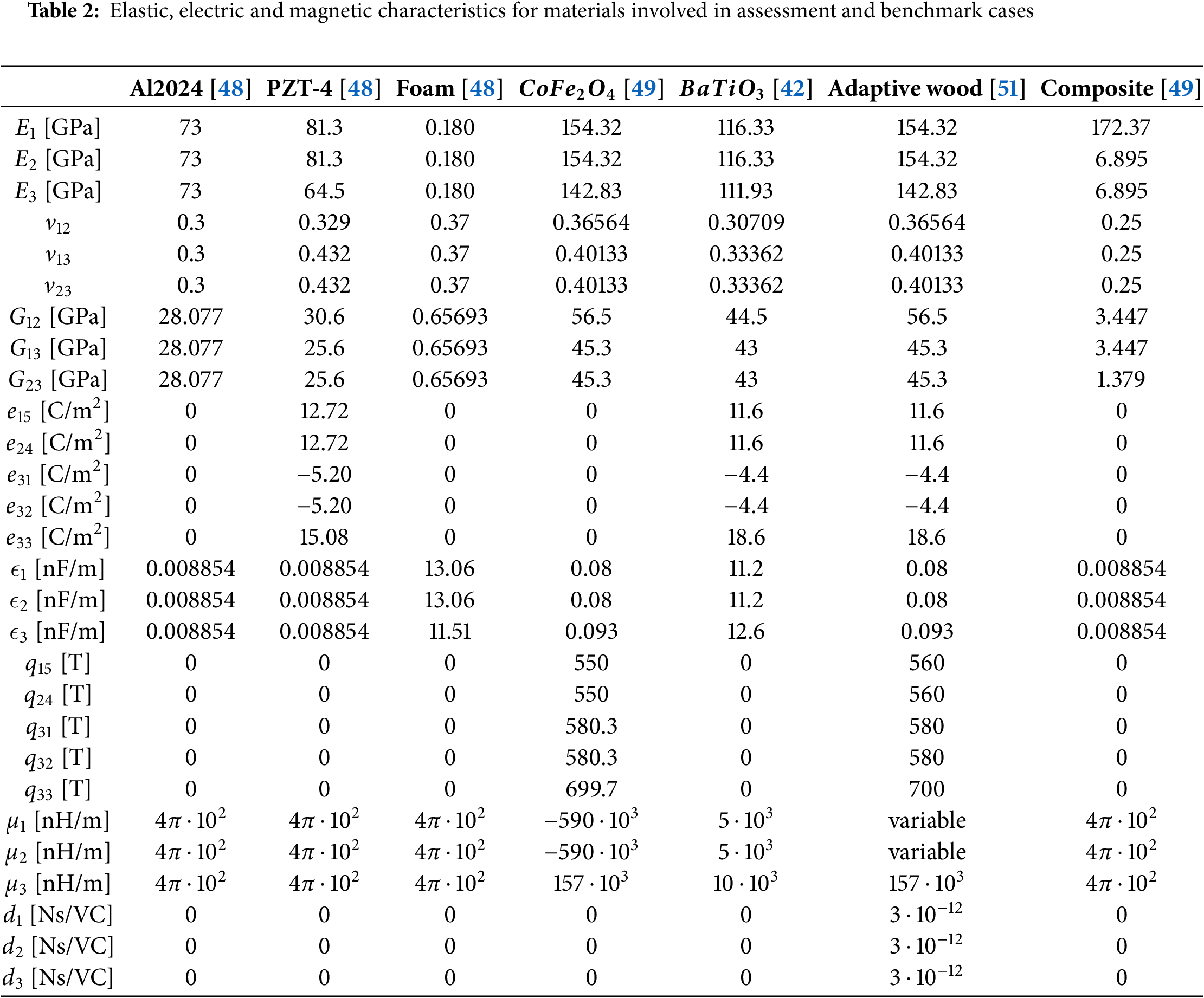
The first assessment (A1) is devoted to a simply supported multilayered square plate in the sensor (A1-S) and actuator (A1-A) configurations. The considered multilayered plate lamination is PZT-4/Al2024/Foam/ Al2024/PZT-4 where hPZT−4=hAl2024=0.1h and hFoam=0.6h where h is the total thickness of the plate. Geometrical data and load conditions are in Table 1 and material properties are collected in Table 2. Elastic properties reported in Table 2 are computed with relations explicitly written for orthotropic materials in [54], starting from the elastic coefficients of the material. The reference solution is the 3D electro-elastic model (3D-u-ϕ model) proposed in [48]. Tables 3 and 4 show comparisons between the present 3D-u-ϕ-ψ model and the 3D-u-ϕ model [48] for both sensor and actuator configurations in terms of displacements, stresses, electric potential, and electric displacement. The accordance between the results is good for each thickness ratio and for each variable proposed. The perfect accordance of results is visible for both primary variables (u, w, ϕ) and secondary variables (σxx, σzz, Dz), certifying the correct computation of each kind of variable. Therefore, this assessment permits validation of the electro-elastic coupling and the thickness and material layer effects in multilayered piezoelectric plates.

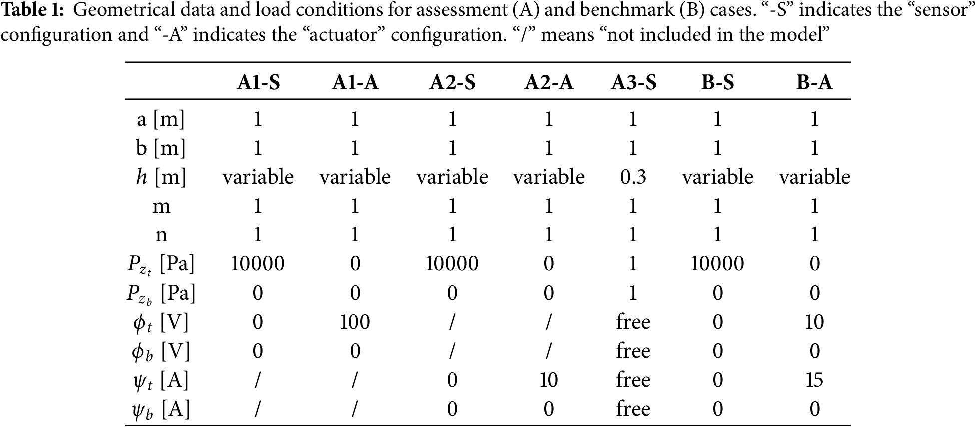
In the second assessment (A2), a multilayered square plate is proposed in both sensor (A2-S) and actuator (A2-A) configurations. In this case, the multilayered plate lamination is CoFe2O4/Al2024/Foam/ Al2024/CoFe2O4 where hCoFe2O4=hAl2024=0.1h and hFoam=0.6h where h is the total thickness of the plate. Geometrical data and load conditions are listed in Table 1. Material properties in terms of magnetic, electric, and mechanical coefficients are detailed in Table 2. The reference solution for both configurations is the 3D-u-ψ magneto-elastic model in [49]. Tables 5 and 6 show results in terms of displacements v and w, stresses σxx and σzz, magnetic potential ψ and magnetic induction ℬz for different thickness locations. A perfect agreement between the 3D-u-ψ-ϕ model and the reference solution is possible to observe for each proposed variable and thickness ratio. Even in A2-S and A2-A cases, the perfect match involves primary variables (v, w, ψ) and secondary variables (σxx, σzz, Bz). The present assessment is useful to validate the magneto-elastic coupling and the thickness and material layer effects in multilayered piezomagnetic plates.

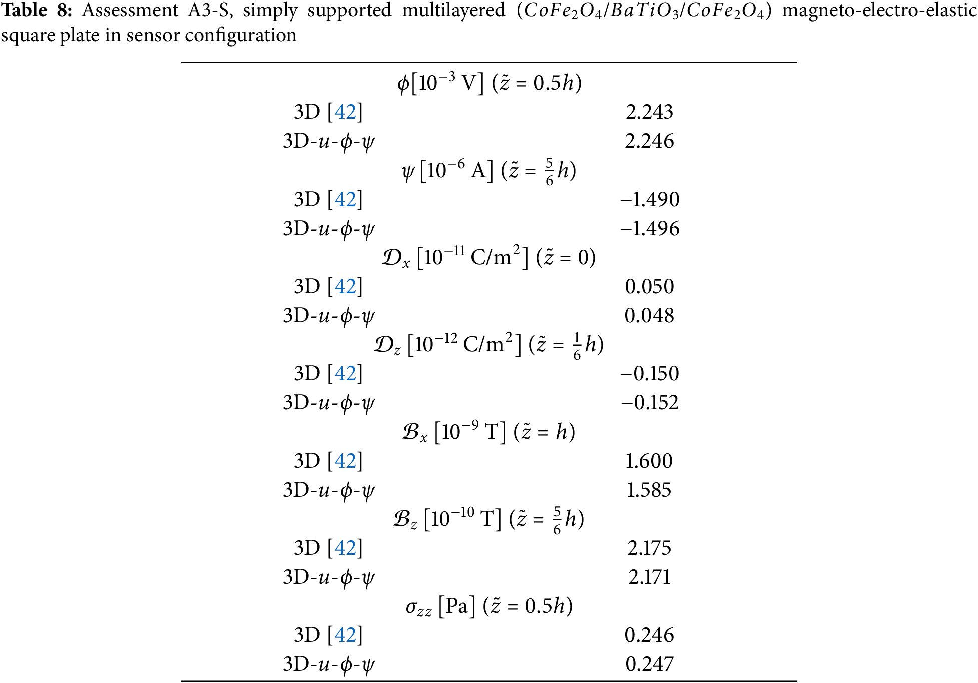
The third assessment (A3) is devoted to a multilayered square plate involving a piezoelectric lamina BaTiO3 and a magnetostrictive lamina CoFe2O4. The first assessed stacking sequence is BaTiO3/CoFe2O4/BaTiO3 and the second one is CoFe2O4/BaTiO3/CoFe2O4 in sensor configuration (A3-S). For both cases, each lamina of the multilayered plate is 0.1m thick. Geometrical data and load boundary conditions are explicitly written in Table 1, while the material properties of the two constituents are listed in Table 2. The reference solution adopted is the 3D magneto-electro-elastic plate model by Pan [42]. Tabular results with four significant digits listed in Tables 7 and 8 were derived from graphical trends proposed in the work [42]. Comparisons for this assessment are presented for ϕ, ψ, 𝒟x, 𝒟z, ℬx, ℬz and σzz variables for both BaTiO3/CoFe2O4/BaTiO3 and CoFe2O4/BaTiO3/CoFe2O4 layered configurations. Tables 7 and 8 exhibit a good match for both stacking sequences between 3D-u-ϕ-ψ model results and the reference ones. Differences in the last digit probably arise from converting in tabular form the results from a graphical trend. Both primary (ϕ, ψ) and secondary (𝒟x, 𝒟z, ℬx, ℬz and σzz) variables are in accordance with the reference results. This assessment is useful to validate the present 3D-u-ϕ-ψ model with a completely different 3D magneto-electro-elastic multilayered plate theory and to validate the fully coupled magneto-electro-elastic effect.

4.2 Benchmarks

This section proposes a new multilayered square plate in both sensor and actuator configurations to evaluate the magneto-electro-elastic coupling effects. The magneto-elastic effects and the electro-elastic effects have already been investigated separately in the assessment part to validate the model. Eight different values for specific z~/h locations are presented for variables w, ϕ, ψ, σxx, σyy, σzz, 𝒟z, and ℬz in tabular forms. z goes from −h/2 to +h/2 and z~ goes from 0 to h. Each variable is proposed for different thickness ratios, from thick (a/h=4) to thin (a/h=100) structures. The same eight variables are also presented in graphical forms along the thickness direction for a moderately thick plate (a/h=10).

This new benchmark considers two different load boundary conditions: sensor configuration (B-S) and the actuator configuration (B-A). From bottom to top, the lamination scheme is Adaptive Wood/0∘/90∘/0∘/Adaptive Wood. Each layer is hAdaptiveWood=0.05h e hComposite=0.3h. h is the total thickness. Geometrical and load conditions are listed in Table 1, and material properties are collected in Table 2. Since in the literature the sign of the magnetic permittivity coefficients μ1 and μ2 are stated as both negative [51] and positive [52], this benchmark is duplicated by considering the two possibilities. So, B-S and B-A are proposed with both μ1=μ2=−590⋅103 nH/m and μ1=μ2=590⋅103 nH/m. In Tables 9–12, variables w, ϕ, ψ, σxx, σyy, σzz, 𝒟z and ℬz are proposed at different z~/h thickness positions and for different a/h thickness ratios for both sensor and actuator cases. Tables 9 and 11 indicate the effect of the sign on permittivity coefficients μ1 and μ2 for the sensor case: slight differences in results onto the electric and magnetic variables (ϕ, 𝒟z, ψ and ℬz) are present. Tables 10 and 12 demonstrate that greater differences in all the proposed variables occur in both thick and thin plates for the actuator configuration due to the different signs of the permittivity coefficients μ1 and μ2. Figs. 2 and 3 depict trends along the thickness direction of the proposed tabular variables, considering negative μ1 and μ2 for the sensor and actuator case, respectively. Figs. 4 and 5 indicate that the same trends are reported considering positive magnetic permittivity coefficients. Both sensor and actuator configurations exhibit that the correct imposition of the load boundary conditions (for the sensor case, σzzt=Pzt=10000 Pa and σzzb=Pzb=0 Pa, ϕt=ϕb=0 V, ψt=ψb=0 A; for the actuator case, σzzt=σzzb=Pzt=Pzb=0 Pa, ϕt=10 V and ϕb=0 V, ψt=15 A and ψb=0 A). In addition, it is clear the perfect depiction of the magneto-electro-elastic coupling for both sensor and actuator cases: in B-S case, the presence of a transverse normal load at the top surface creates a ϕ electric potential and a ψ magnetic potential in the thickness of the plate, in the B-A case, the ϕ electric potential trend and the ψ magnetic potential trend in the thickness of the plate generates a σzz non-zero trend along the thickness direction. For each presented variable, the zigzag effect is shown as a multilayered structure is analyzed. The zigzag effect is apparent for both configurations as the slope drastically changes in correspondence with the physical interfaces of the plate. For variables w, ϕ, ψ, σzz, 𝒟z, and ℬz trends are continuous along the thickness direction owning to the correct imposition of interlaminar continuity conditions at each interface between two adjacent k layers. For variables σxx and σyy, trends are discontinuous as no interlaminar continuity conditions are imposed. For the sensor configuration, the sign of the magnetic permittivity coefficients μ1 and μ2 only affects the ℬz trend (Figs. 2 and 4). In the case of the actuator configuration, different trends are due to the different signs of the magnetic permittivity regarding the w displacement, the σxx and σyy stresses and the ℬz transverse magnetic induction (Figs. 3 and 5). The sign of μ1 and μ2 coefficients does not affect any of the previously described peculiarities related to the model (load boundary conditions, magneto-electro-elastic coupling effect, zigzag effect and interlaminar continuity conditions).

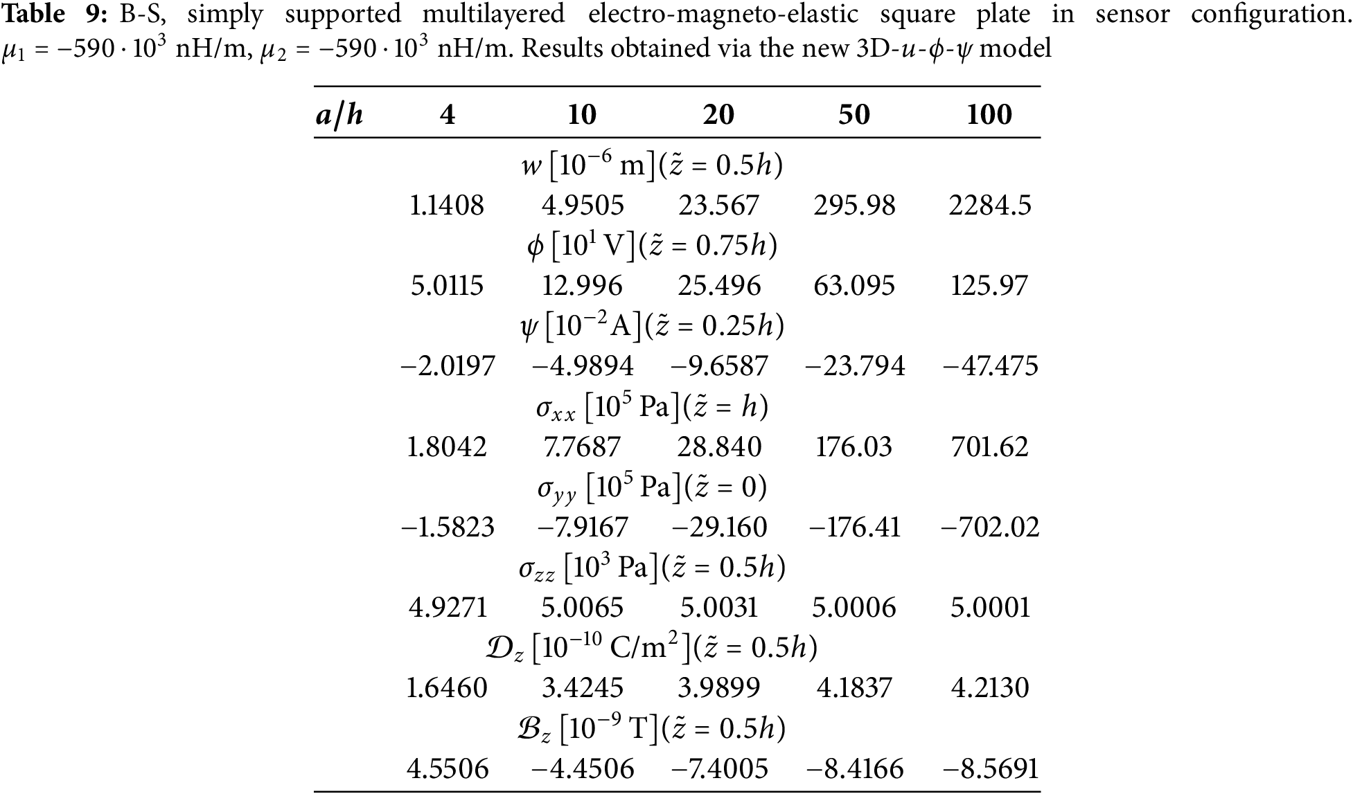
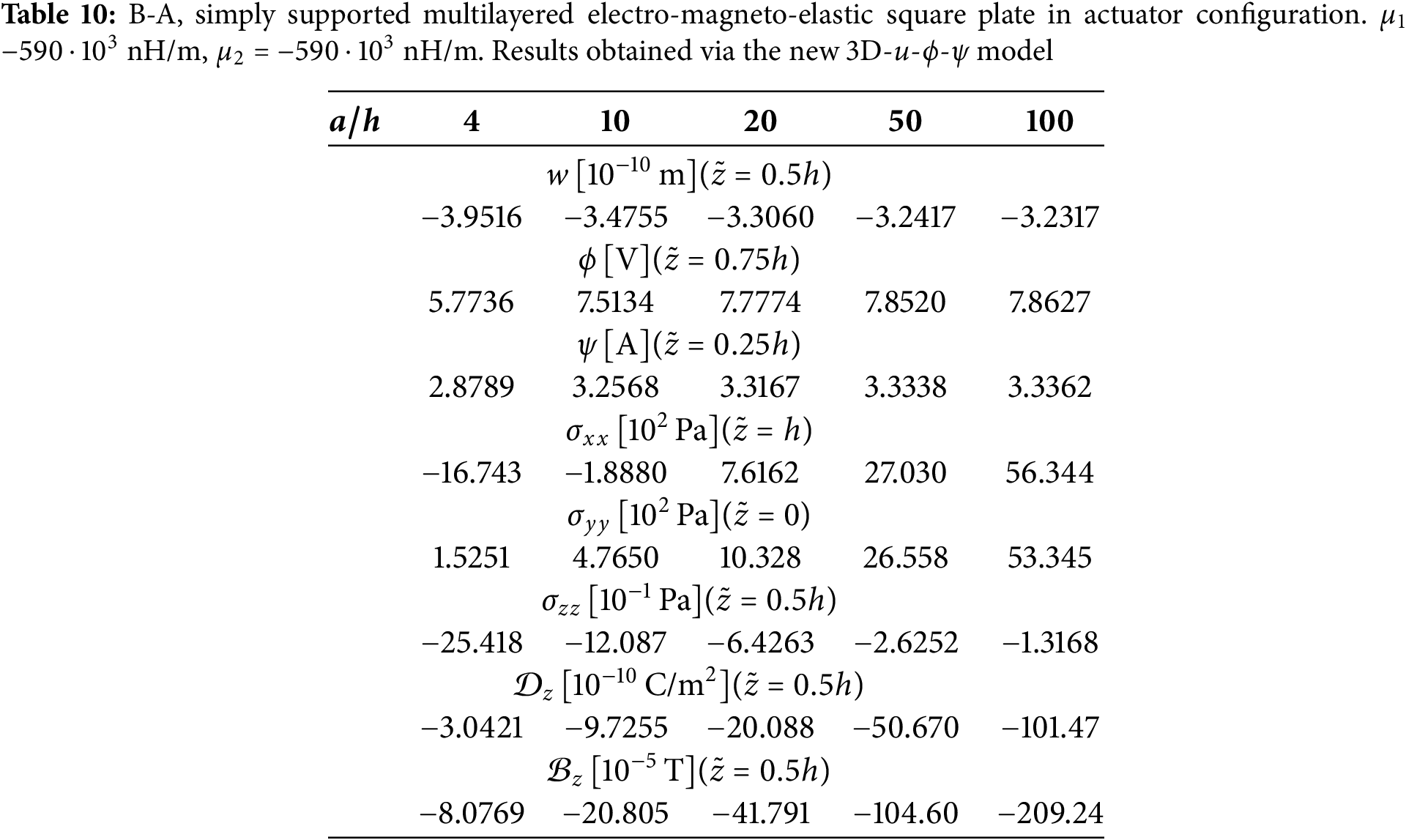
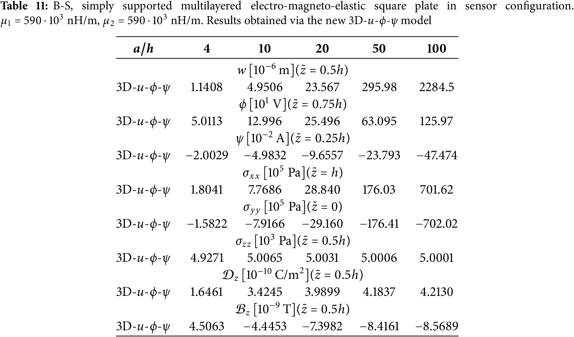
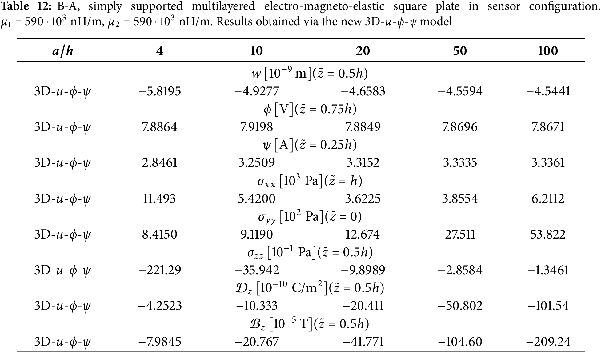
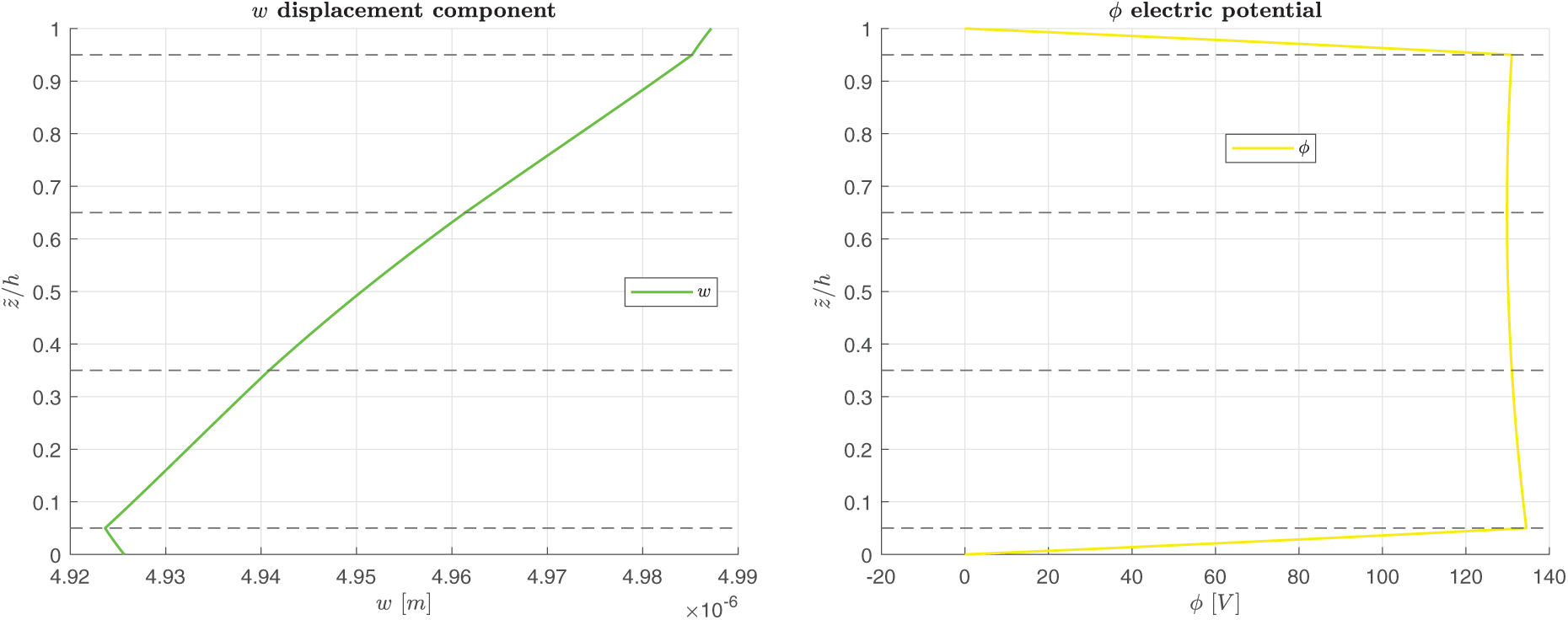
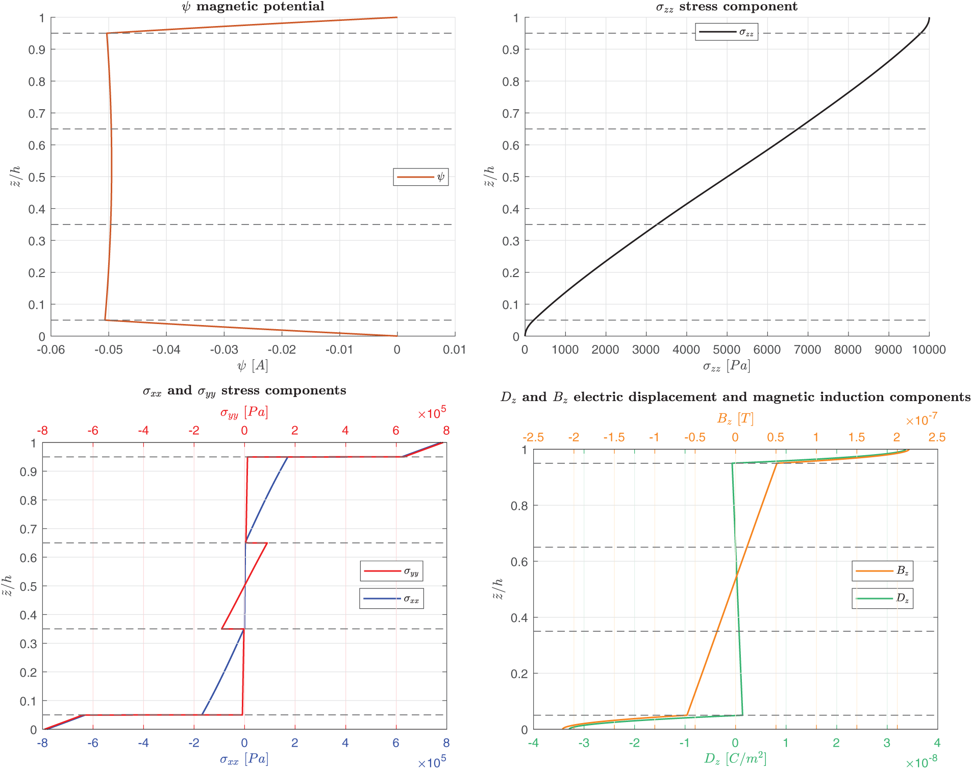
Figure 2: B-S, simply-supported multilayered electro-magneto-elastic square plate in sensor configuration. μ1=−590⋅103 nH/m, μ2=−590⋅103 nH/m. Results obtained via the new 3D-u-ϕ-ψ model for thickness ratio a/h=10

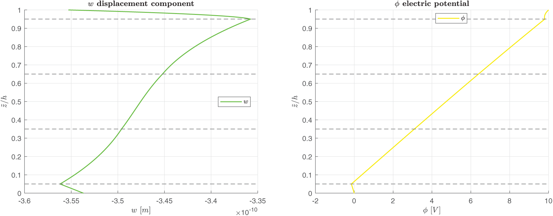
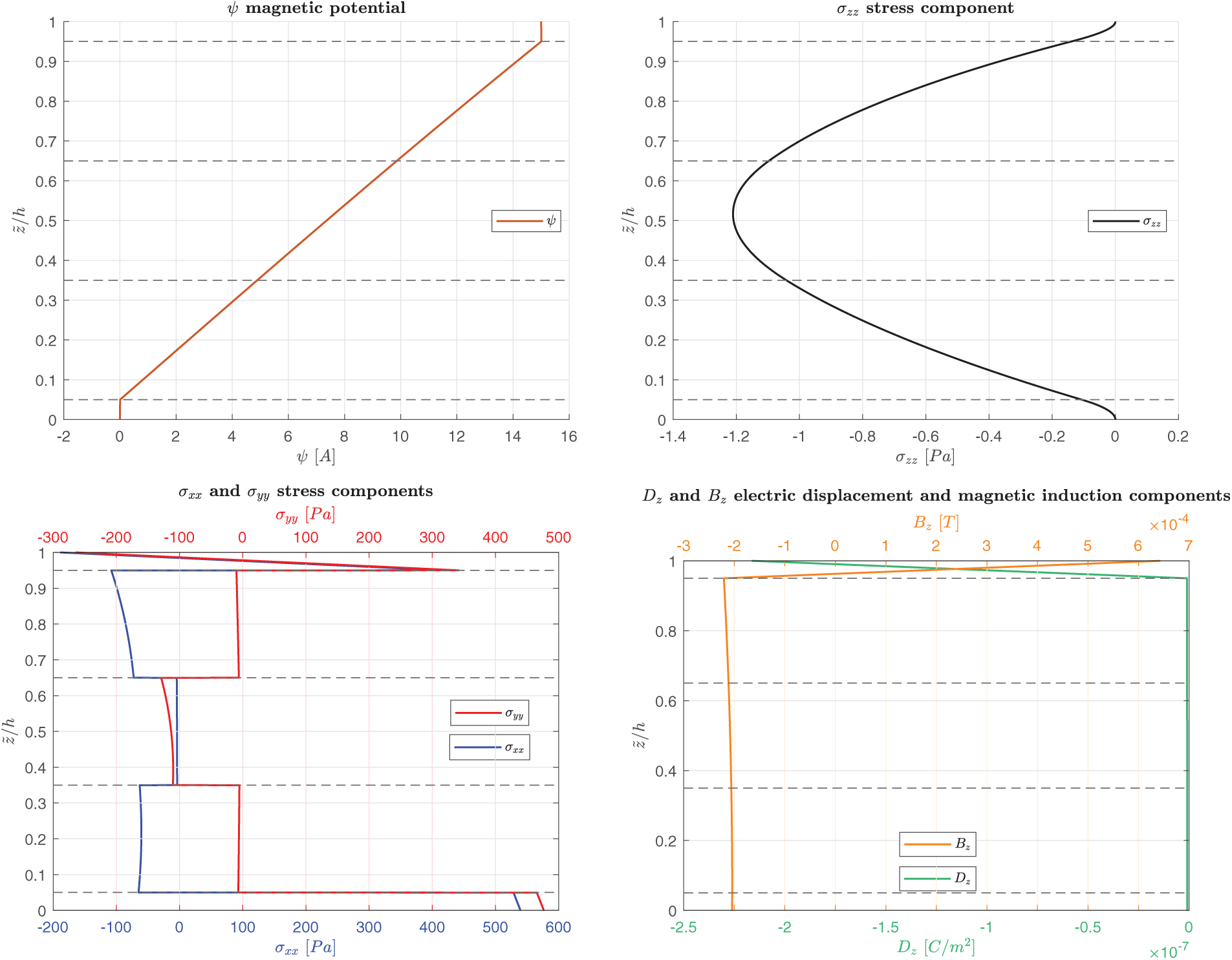
Figure 3: B-A, simply-supported multilayered electro-magneto-elastic square plate in actuator configuration. μ1=−590⋅103 nH/m, μ2=−590⋅103 nH/m. Results obtained via the new 3D-u-ϕ-ψ model for thickness ratio a/h=10

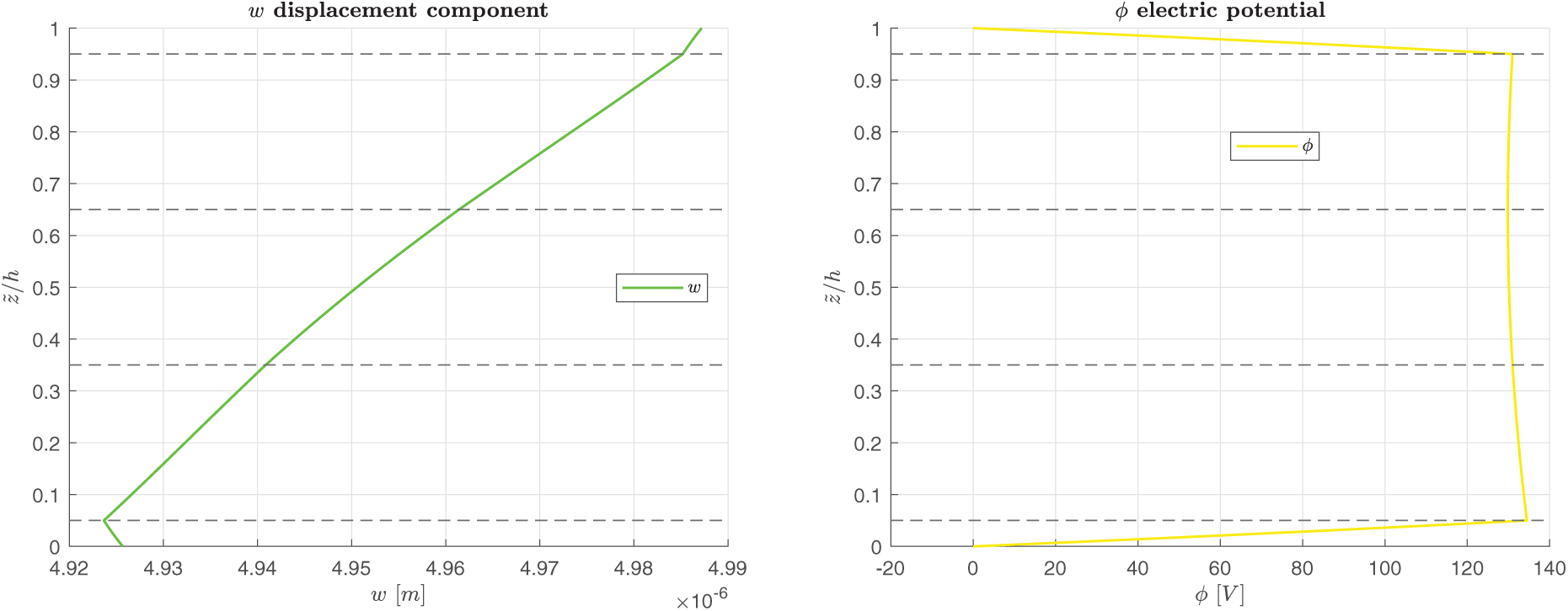
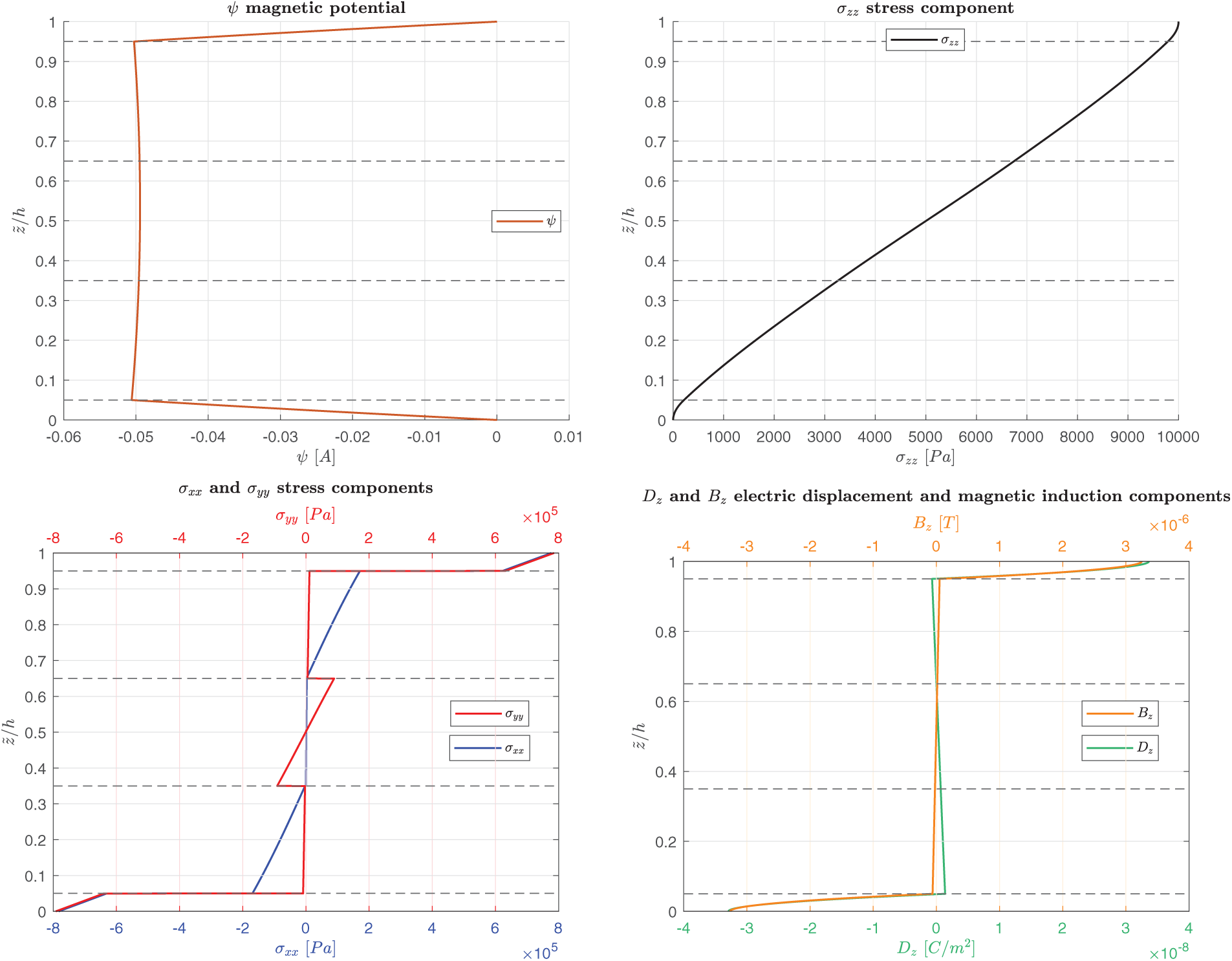
Figure 4: B-S, simply-supported multilayered electro-magneto-elastic square plate in sensor configuration. μ1=590⋅103 nH/m, μ2=590⋅103 nH/m. Results obtained via the new 3D-u-ϕ-ψ model for thickness ratio a/h=10

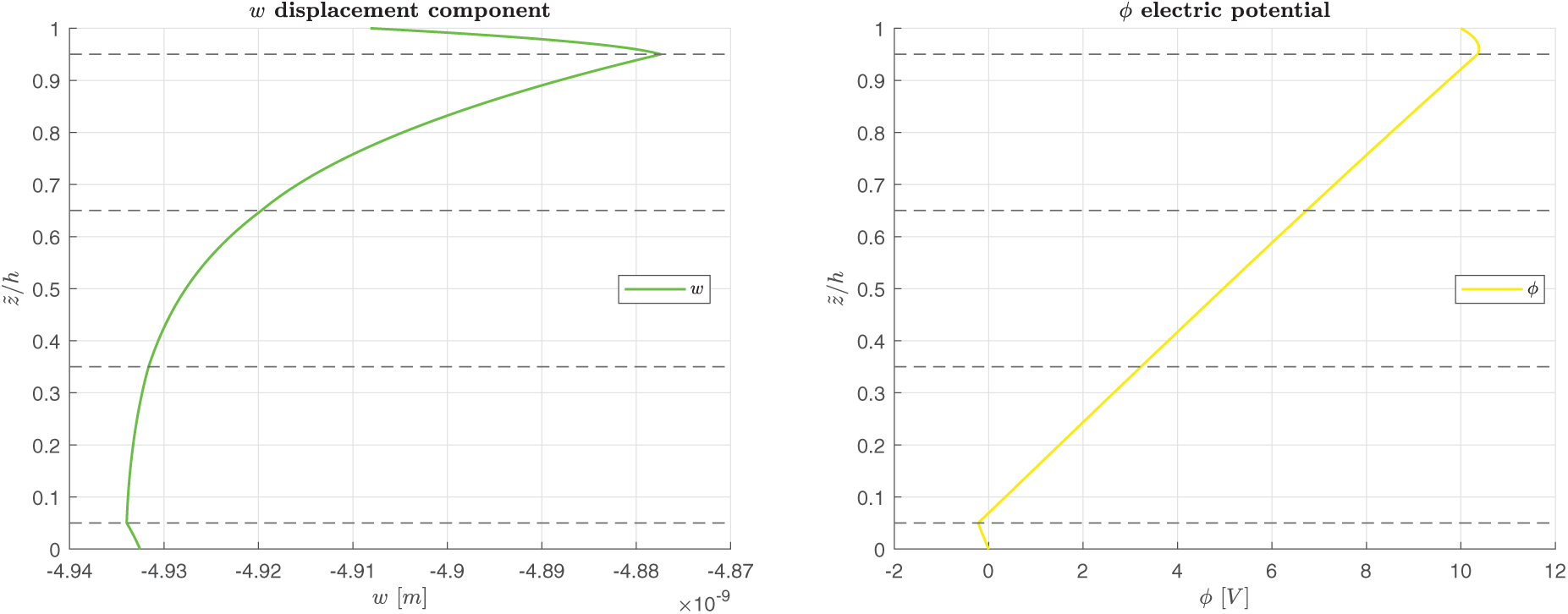
Figure 5: B-A, simply-supported multilayered electro-magneto-elastic square plate in actuator configuration. μ1=590⋅103 nH/m, μ2=590⋅103 nH/m. Results obtained via the new 3D-u-ϕ-ψ model for thickness ratio a/h=10

5  Conclusions

This study proposes an exact 3D, fully coupled magneto-electro-elastic model for multilayered plates where the three 3D equilibrium equations, the 3D divergence equation for magnetic induction, and the 3D divergence equation for electric induction are the 3D governing equation of the magneto-electro-elastic model. Solution methodology considers Navier harmonic forms in the in-plane directions and the exponential matrix method in the thickness direction. A closed form solution is performed, and only simply supported boundary conditions are possible. In addition, only orthotropic laminae involving piezoelectric and/or piezomagnetic characteristics can be considered. Due to the imposition of the interlaminar continuity conditions between two adjacent layers, the layerwise approach is adopted. In the assessment subsection, the present model is validated with other 3D plate models involving magneto-elastic or electro-elastic effects in a separate way. In the second part, new results are presented in sensor and actuator configurations for different thickness ratios in the case of full coupling between electric, magnetic, and elastic fields. The benchmark case is proposed firstly considering both coefficients with a positive sign and then with a negative sign, to overcome the literature misunderstanding about the proper sign of the magnetic permittivity coefficients μ1 and μ2. The present 3D magneto-electro-elastic model correctly depicts the magneto-electro-elastic coupling, the thickness and material layer effects and the load conditions for all thickness ratios considered. Load boundary conditions are correctly implemented for both sensor and actuator configurations. The present 3D magneto-electro-elastic model can be utilized to understand the behavior of smart multilayered plates embedding piezoelectric and piezomagnetic materials.

Acknowledgement: Not applicable.

Funding Statement: The authors received no specific funding for this study.

Author Contributions: The authors confirm contribution to the paper as follows: Conceptualization, Salvatore Brischetto; methodology, Salvatore Brischetto; software, Tommaso Mondino; validation, Tommaso Mondino; formal analysis, Salvatore Brischetto; investigation, Domenico Cesare; resources, Domenico Cesare; data curation, Domenico Cesare; writing—original draft preparation, Domenico Cesare; writing—review and editing, Salvatore Brischetto and Domenico Cesare; visualization, Domenico Cesare; supervision, Salvatore Brischetto. All authors reviewed the results and approved the final version of the manuscript.

Availability of Data and Materials: Not applicable.

Ethics Approval: Not applicable.

Conflicts of Interest: The authors declare no conflicts of interest to report regarding the present study.

References

1. Bichurin M, Petrov V, Tatarenko A. Predicting magnetoelectric coupling in layered and graded composites. Sensors. 2017;17(7):1651. doi:10.3390/s17071651. [Google Scholar] [PubMed] [CrossRef]

2. Jiang Z, Zhang F, Li K, Chai Y, Li W, Gui Q. A multi-physics overlapping finite element method for band gap analyses of the magneto-electro-elastic radial phononic crystal plates. Thin-Walled Struct. 2025;210(4):112985. doi:10.1016/j.tws.2025.112985. [Google Scholar] [CrossRef]

3. Liu C, Li K, Min S, Chai Y. Dynamic analysis of the three-phase magneto-electro-elastic (MEE) structures with the overlapping triangular finite elements. Comput Math Appl. 2025;179:148–77. doi:10.1016/j.camwa.2024.11.025. [Google Scholar] [CrossRef]

4. Milazzo A, Orlando C. A beam finite element for magneto-electro-elastic multilayered composite structures. Compos Struct. 2012;94(12):3710–21. doi:10.1016/j.compstruct.2012.06.011. [Google Scholar] [CrossRef]

5. Shakeel M, Attaullah, Alaoui MK, Zidan AM, Shah NA, Weera W. Closed-form solutions in a magneto-electro-elastic circular rod via generalized exp-function method. Math. 2012;10(18):3400. doi:10.3390/math10183400. [Google Scholar] [CrossRef]

6. Hong J, Wang S, Zhang G, Mi C. On the bending and vibration analysis of functionally graded magneto-electro-elastic Timoshenko microbeams. Crystals. 2021;11(10):1206. doi:10.3390/cryst11101206. [Google Scholar] [CrossRef]

7. Nixdorf TA, Pan E. Static plane-strain deformation of transversely isotropic magneto-electro-elastic and layered cylinders to general surface loads. Appl Math Model. 2018;60:208–19. doi:10.1016/j.apm.2018.03.018. [Google Scholar] [CrossRef]

8. Huang DJ, Ding HJ, Chen WQ. Static analysis of anisotropic functionally graded magneto-electro-elastic beams subjected to arbitrary loading. Eur J Mech A/Solids. 2010;29(3):356–69. doi:10.1016/j.euromechsol.2009.12.002. [Google Scholar] [CrossRef]

9. Chen J, Chen H, Pan E, Heyliger PR. Modal analysis of magneto-electro-elastic plates using the state-vector approach. J Sound Vib. 2007;304(3–5):722–34. doi:10.1016/j.jsv.2007.03.021. [Google Scholar] [CrossRef]

10. Phoenix SS, Satsangi SK, Singh BN. Layer-wise modelling of magneto-electro-elastic plates. J Sound Vib. 2009;324(3–5):798–815. doi:10.1016/j.jsv.2009.02.025. [Google Scholar] [CrossRef]

11. Zhou L, Chen P, Gao Y, Wang J. Mechanical-electric-magnetic-thermal coupled enriched finite element method for magneto-electro-elastic structures. Model Simul Mater Sci Eng. 2024;32(7):075010. doi:10.1088/1361-651x/ad747c. [Google Scholar] [CrossRef]

12. Rao MN, Schmidt R, Schroder K-U. Geometrically nonlinear static FE-simulation of multilayered magneto-electro-elastic composite structures. Compos Struct. 2015;127(7104):120–31. doi:10.1016/j.compstruct.2015.03.002. [Google Scholar] [CrossRef]

13. Wang J, Zhou L, Chai Y. The adaptive hygrothermo-magneto-electro-elastic coupling improved enriched finite element method for functionally graded magneto-electro-elastic structures. Thin-Walled Struct. 2024;200(7104):111970. doi:10.1016/j.tws.2024.111970. [Google Scholar] [CrossRef]

14. Carrera E, Di Gifico M, Nali P, Brischetto S. Refined multilayered plate elements for coupled magneto-electro-elastic analysis. Multidiscip Model Mater Struct. 2009;5(2):119–38. doi:10.1163/157361109787959859. [Google Scholar] [CrossRef]

15. Carrera E, Brischetto S, Fagiano C, Nali P. Mixed multilayered plate elements for coupled magneto-electro-elastic analysis. Multidiscip Model Mater Struct. 2009;5(3):251–6. doi:10.1163/157361109789017050. [Google Scholar] [CrossRef]

16. Liu M-F. An exact deformation analysis for the magneto-electro-elastic fiber-reinforced thin plate. Appl Math Model. 2011;35(5):2443–61. doi:10.1016/j.apm.2010.11.044. [Google Scholar] [CrossRef]

17. Milazzo A. Large deflection of magneto-electro-elastic laminated plates. Appl Math Model. 2014;38(5–6):1737–52. doi:10.1016/j.apm.2013.08.034. [Google Scholar] [CrossRef]

18. Alaimo A, Milazzo A, Orlando C. A four-node MITC finite element for magneto-electro-elastic multilayered plates. Comput Struct. 2013;129:120–33. doi:10.1016/j.compstruc.2013.04.014. [Google Scholar] [CrossRef]

19. Alaimo A, Benedetti I, Milazzo A. A finite element formulation for large deflection of multilayered magneto-electro-elastic plates. Compos Struct. 2014;107(1):643–53. doi:10.1016/j.compstruct.2013.08.032. [Google Scholar] [CrossRef]

20. Chen JY, Pan E, Heyliger PR. Static deformation of a spherically anisotropic and multilayered magneto-electro-elastic hollow sphere. Int J Solids Struct. 2015;60–61:66–74. doi:10.1016/j.ijsolstr.2015.02.004. [Google Scholar] [CrossRef]

21. Garcia Lage R, Mota Soares CM, Mota Soares CA, Reddy JN. Layerwise partial mixed finite element analysis of magneto-electro-elastic plates. Comput Struct. 2004;82(17–19):1293–301. doi:10.1016/j.compstruc.2004.03.026. [Google Scholar] [CrossRef]

22. Hsu C-W, Hwu C. Classical solutions for coupling analysis of unsymmetric magneto-electro-elastic composite laminated thin plates. Thin-Walled Struct. 2022;181:110112. doi:10.1016/j.tws.2022.110112. [Google Scholar] [CrossRef]

23. Liu J, Zhang P, Lin G, Wang W, Lu S. Solutions for the magneto-electro-elastic plate using the scaled boundary finite element method. Eng Anal Bound Elem. 2016;68(4):103–14. doi:10.1016/j.enganabound.2016.04.005. [Google Scholar] [CrossRef]

24. Zhou L, Yang H, Ma L, Zhang S, Li X, Ren S, et al. On the static analysis of inhomogeneous magneto-electro-elastic plates in thermal environment via element-free Galerkin method. Eng Anal Bound Elem. 2022;134(1):539–52. doi:10.1016/j.enganabound.2021.11.002. [Google Scholar] [CrossRef]

25. Chen H, Yu W. A multiphysics model for magneto-electro-elastic laminates. Eur J Mech A/Solids. 2014;47(6):23–44. doi:10.1016/j.euromechsol.2014.02.004. [Google Scholar] [CrossRef]

26. Ntayeesh TJ, Arefi M. Analysis of sandwich graphene origami composite plate sandwiched by piezoelectric/piezomagnetic layers: a higher-order electro-magneto-elastic analysis. Heliyon. 2024;10(8):e29436. doi:10.1016/j.heliyon.2024.e29436. [Google Scholar] [PubMed] [CrossRef]

27. Kiarasi F, Babaei M, Asemi K, Dimitri R, Tornabene F. Free vibration analysis of thick annular functionally graded plate integrated with piezo-magneto-electro-elastic layers in a hygrothermal environment. Appl Sci. 2022;12(20):10682. doi:10.3390/app122010682. [Google Scholar] [CrossRef]

28. Tocci Monaco G, Fantuzzi N, Fabbrocino F, Luciano R. Trigonometric solution for the bending analysis of magneto-electro-elastic strain gradient nonlocal nanoplates in hygro-thermal environment. Mathematics. 2021;9(5):567. doi:10.3390/math9050567. [Google Scholar] [CrossRef]

29. Tocci Monaco G, Fantuzzi N, Fabbrocino F, Luciano R. Critical temperatures for vibrations and buckling of magneto-electro-elastic nonlocal strain gradient plates. Nanomater. 2021;11(1):87. doi:10.3390/nano11010087. [Google Scholar] [PubMed] [CrossRef]

30. Zhang B, Yu J, Elmaimouni L, Zhang X. Magneto-electric effect on guided waves in functionally graded piezoelectric-piezomagnetic fan-shaped cylindrical structures. Materials. 2018;11(11):2174. doi:10.3390/ma11112174. [Google Scholar] [PubMed] [CrossRef]

31. Anh VTT, Dat ND, Nguyen PD, Duc ND. A nonlocal higher-order shear deformation approach for nonlinear static analysis of magneto-electro-elastic sandwich micro/nano-plates with FG-CNT core in hygrothermal environment. Aerosp Sci Technol. 2024;147(11):109069. doi:10.1016/j.ast.2024.109069. [Google Scholar] [CrossRef]

32. Zhang P, Qi C, Fang H, Ma C, Huang Y. Semi-analytical analysis of static and dynamic responses for laminated magneto-electro-elastic plates. Compos Struct. 2019;222(2):110933. doi:10.1016/j.compstruct.2019.110933. [Google Scholar] [CrossRef]

33. Jiang W-W, Gao X-W, Liu H-Y. Multi-physics zonal Galerkin free element method for static and dynamic responses of functionally graded magneto-electro-elastic structures. Compos Struct. 2023;321(21):117217. doi:10.1016/j.compstruct.2023.117217. [Google Scholar] [CrossRef]

34. Zhou L, Qu F. The magneto-electro-elastic coupling isogeometric analysis method for the static and dynamic analysis of magneto-electro-elastic structures under thermal loading. Compos Struct. 2023;315(21):116984. doi:10.1016/j.compstruct.2023.116984. [Google Scholar] [CrossRef]

35. Tornabene F, Viscoti M, Dimitri R. Equivalent layer-wise theory for the hygro-thermo-magneto-electro-elastic analysis of laminated curved shells. Thin-Walled Struct. 2024;198(103136):111751. doi:10.1016/j.tws.2024.111751. [Google Scholar] [CrossRef]

36. Tornabene F, Viscoti M, Dimitri R. Magneto-electro-elastic analysis of doubly-curved shells: higher-order equivalent layer-wise formulation. Comput Model Eng Sci. 2025;142(2):1767–838. doi:10.32604/cmes.2024.058842. [Google Scholar] [CrossRef]

37. Ren S, Mahesh V, Meng G, Zhou L. Static responses of magneto-electro-elastic structures in moisture field using stabilized node-based smoothed radial point interpolation method. Compos Struct. 2020;252:112696. doi:10.1016/j.compstruct.2020.112696. [Google Scholar] [CrossRef]

38. Kuang Z-B. Physical variational principle and thin plate theory in electro-magneto-elastic analysis. Int J Solids Struct. 2011;48(2):317–25. doi:10.1016/j.ijsolstr.2010.10.008. [Google Scholar] [CrossRef]

39. Li XY, Ding HJ, Chen WQ. Three-dimensional analytical solution for functionally graded magneto-electro-elastic circular plates subjected to uniform load. Compos Struct. 2008;83(4):381–90. doi:10.1016/j.compstruct.2007.05.006. [Google Scholar] [CrossRef]

40. Wang R, Han Q, Pan E. An analytical solution for a multilayered magneto-electro-elastic circular plate under simply supported lateral boundary conditions. Smart Mater Struct. 2010;19(4):065025. doi:10.1115/1.1380385. [Google Scholar] [CrossRef]

41. Gong Z, Zhang Y, Pan E, Zhang C. Three-dimensional general magneto-electro-elastic finite element model for multiphysics nonlinear analysis of layered composites. Appl Math Mech. 2023;44(1):53–72. doi:10.1007/s10483-023-2943-8. [Google Scholar] [CrossRef]

42. Pan E. Exact solution for simply supported and multilayered magneto-electro-elastic plates. J Appl Mech. 2001;68(4):608–18. doi:10.1115/1.1380385. [Google Scholar] [CrossRef]

43. Wang J, Chen L, Fang S. State vector approach to analysis of multilayered magneto-electro-elastic plates. Int J Solids Struct. 2003;40(7):1669–80. doi:10.1016/s0020-7683(03)00027-1. [Google Scholar] [CrossRef]

44. Vinyas M, Kattimani SC. Hygrothermal analysis of magneto-electro-elastic plate using 3D finite element analysis. Compos Struct. 2017;180(1):617–37. doi:10.1016/j.compstruct.2017.08.015. [Google Scholar] [CrossRef]

45. Pan E, Heyliger PR. Free vibrations of simply supported and multilayered magneto-electro-elastic plates. J Sound Vib. 2002;252(3):429–42. doi:10.1006/jsvi.2001.3693. [Google Scholar] [CrossRef]

46. Wu C-P, Chen S-J, Chiu K-H. Three-dimensional static behavior of functionally graded magneto-electro-elastic plates using the modified Pagano method. Mech Res Commun. 2010;37(1):54–60. doi:10.1016/j.mechrescom.2009.10.003. [Google Scholar] [CrossRef]

47. Wu C-P, Tsai Y-H. Static behavior of functionally graded magneto-electro-elastic shells under electric displacement and magnetic flux. Int J Eng Sci. 2007;45(9):744–69. doi:10.1016/j.ijengsci.2007.05.002. [Google Scholar] [CrossRef]

48. Brischetto S, Cesare D. 3D electro-elastic static analysis of advanced plates and shells. Int J Mech Sci. 2024;280:109620. doi:10.1016/j.ijmecsci.2024.109620. [Google Scholar] [CrossRef]

49. Brischetto S, Cesare D. A 3D shell model for static and free vibration analysis of multilayered magneto-elastic structures. Thin-Walled Struct. 2025;206(7):112620. doi:10.1016/j.tws.2024.112620. [Google Scholar] [CrossRef]

50. Brischetto S. A closed-form 3D shell solution for multilayered structures subjected to different load combinations. Aerosp Sci Technol. 2017;70:29–46. doi:10.1016/j.ast.2017.07.040. [Google Scholar] [CrossRef]

51. Tornabene F. Hygro-thermo-magneto-electro-elastic theory of anisotropic doubly-curved shells. Bologna, Italy: Societa’ Editrice Esculapio; 2023. [Google Scholar]

52. Pan E. Three-dimensional Green’s functions in anisotropic magneto-electro-elastic bimaterials. Zeitschrift FÄur Angewandte Mathematik Und Physik. 2002;53:815–38. [Google Scholar]

53. Brischetto S. Convergence analysis of the exponential matrix method for the solution of 3D equilibrium equations for free vibration analysis of plates and shells. Composites Part B. 2016;98:453–71. doi:10.1016/j.compositesb.2016.05.047. [Google Scholar] [CrossRef]

54. Reddy JN. Mechanics of laminated composite plates and shells. In: Theory and analysis. Boca Raton, FL, USA: CRC Press; 2003. [Google Scholar]