CGAN Accelerated Subdivision Surface BEM for Acoustic Scattering

1  Introduction

Nowadays, widely used numerical tools such as finite element methods (FEM) [1–5] and boundary element methods (BEM) [6–9] rely heavily on geometric fidelity to ensure reliable structural and acoustic simulations. Recent advances integrate computer-aided design (CAD) techniques—including nonuniform rational B-splines (NURBS) [10], T-splines [11], and subdivision surfaces [12,13]—to bridge the gap between geometric modeling and numerical analysis. Among these, subdivision surfaces offer a distinct advantage for complex topologies. Unlike NURBS, which require laborious surface stitching to maintain continuity [14], subdivision schemes iteratively refine coarse polygonal meshes into smooth limit surfaces, inherently preserving geometric continuity without manual intervention.

Early subdivision methods, including Catmull-Clark [15], Loop [16], and Butterfly [17], have been widely adopted in 3D modeling and structural analysis. Among these, the Loop subdivision scheme stands out for its ability to handle complex geometries with sharp features or discontinuities. By reconstructing an initial coarse mesh (Fig. 1a), the algorithm iteratively refines the topology to generate smooth limit surfaces (Fig. 1c) with minimal subdivision steps. This efficiency, achieving visually smooth results in just a few iterations, demonstrates the computational advantage of Loop subdivision over traditional meshing techniques. Subdivision surfaces [18,19] are uniquely suited for engineering applications due to their ability to model arbitrary topological structures while maintaining strict control over computational and storage costs. Unlike conventional spline-based approaches, subdivision operates through local refinement rules, enabling scalable and adaptive geometric representations [20,21]. These properties make subdivision surfaces, and the Loop scheme in particular, a robust foundation for isogeometric analysis, where seamless integration of geometric modeling and numerical discretization is critical.

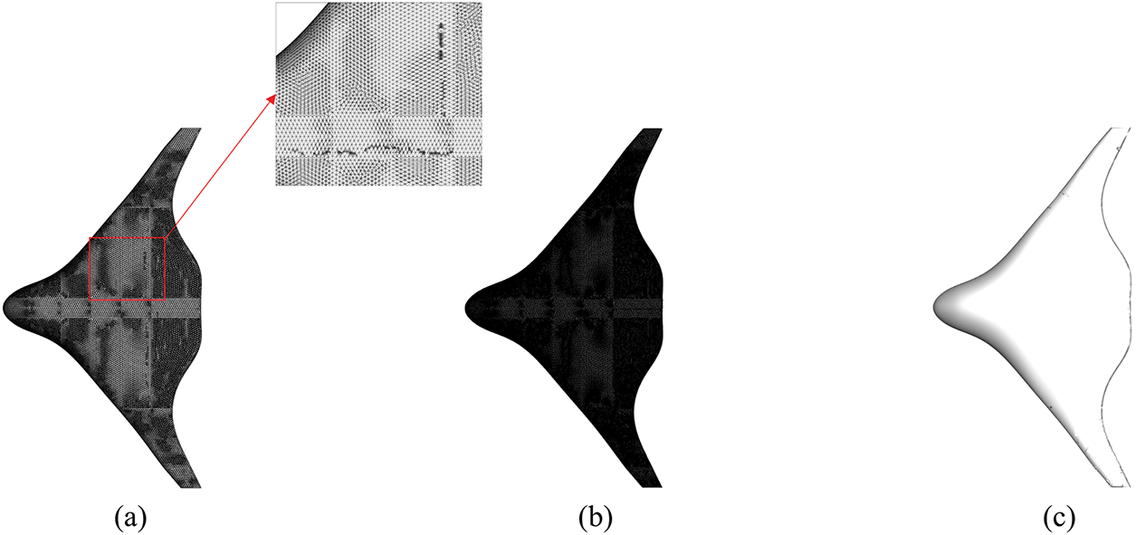
Figure 1: The initial mesh model (a), the model refined by the subdivision surface (b), and the limit surface model (c), with smooth transitions at the joints

Compared to finite element methods (FEM), the boundary element method (BEM) [22] offers a critical advantage through dimensionality reduction [23], as it discretizes only the boundary of the domain rather than the entire volume. This property makes BEM particularly effective for solving wave propagation and scattering problems in infinite or semi-infinite domains. For exterior acoustic scattering governed by the Helmholtz equation, BEM inherently satisfies the Sommerfeld radiation condition at infinity [24], eliminating the need for artificial absorbing boundary layers required in FEM.

However, BEM’s reliance on dense matrix assembly—a consequence of its Green function-based formulation—poses significant computational challenges for large-scale problems. Recent advances address this through hierarchical acceleration techniques such as the fast multipole method (FMM) [6,25], which reduces computational complexity from O(N2) to O(NlogN). Further efficiency gains are achieved by integrating subdivision surfaces with BEM [22], allowing adaptive geometric refinement without repeated regeneration of the mesh. This approach automatically generates hierarchical models (Fig. 1) that balance accuracy and computational cost during pre-processing. Despite these advancements, two critical bottlenecks persist:

•   Escalating computational load with increasing subdivision iterations, as finer meshes amplify matrix size and increase computation time.

•   Hardware limitations, where memory constraints and serial processing bottlenecks hinder large-scale simulations, even with FMM acceleration.

Aiming at such challenges, recent advances in deep learning have demonstrated its potential for acoustic simulations: Qu et al. [26] employed deep neural networks (DNNs) for data augmentation and accelerated uncertainty quantification. Chen et al. [27] conducted rapid analysis of uncertainties arising from different material parameters in acoustic-vibration coupling problems using a simple neural network model. Meanwhile, Zhou et al. [28] accelerated vibroacoustic analysis and proposed a neural network-based method to expedite numerical computations, collectively showcasing deep learning’s efficacy in computational acoustics. Building on these foundations, Conditional Generative Adversarial Networks (CGANs) offer unique advantages for frequency-domain optimization, including targeted data augmentation within user-defined frequency bands [29] and high-fidelity prediction of acoustic fields. The prior application [30] of CGANs in the field of structural acoustics [31] has preliminarily validated their practicality, but their integration with subdivision surface BEM remains unexplored. This study introduces CGANs into boundary element computations for the first time, exploring their feasibility in numerical simulations. By using small-scale datasets to predict large-scale data, CGANs serve as a secondary acceleration strategy to assist traditional numerical computations. CGANs still lack rigorous theoretical proof in numerical computations and currently have only partial empirical applications. Therefore, in this study, CGANs are embedded into the numerical simulation workflow as an auxiliary tool to improve overall computational efficiency.

The structure of this paper is as follows: Section 2 introduces the Loop-based subdivision surface method. Section 3 presents a boundary element discretization method for Helmholtz analysis based on subdivision basis functions. Section 4 describes the CGAN-based accelerated computation approach. Section 5 demonstrates the effectiveness of the proposed method through numerical simulation examples. Finally, Section 6 summarizes the conclusions of this study.

2  Methods of Loop Subdivision

In this study, the isogeometric analysis (IGA) framework is integrated with loop subdivision surfaces for high-fidelity mesh generation, conducted prior to numerical simulation [32]. The loop subdivision method refines triangular elements by iteratively subdividing edges and faces [33]. As illustrated in Fig. 2, the subdivision process begins by inserting midpoints along each edge. Connecting these midpoints divides the original triangular element into four smaller triangles. The valence (nv), defined as the number of edges incident to a vertex, distinguishes regular vertices (nv=6) from irregular vertices (nv≠6). The Loop scheme produces C2-continuous surfaces at regular vertices and C1-continuous surfaces at irregular vertices. The refinement process is further detailed in Fig. 3, where:

•   At subdivision level k, a new vertex xek+1 is inserted at the midpoint of each edge.

•   The position of each original vertex from level k is denoted as xvk+1.

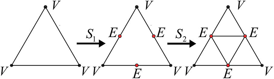
Figure 2: The positions of edge points “E” and vertex points “V”

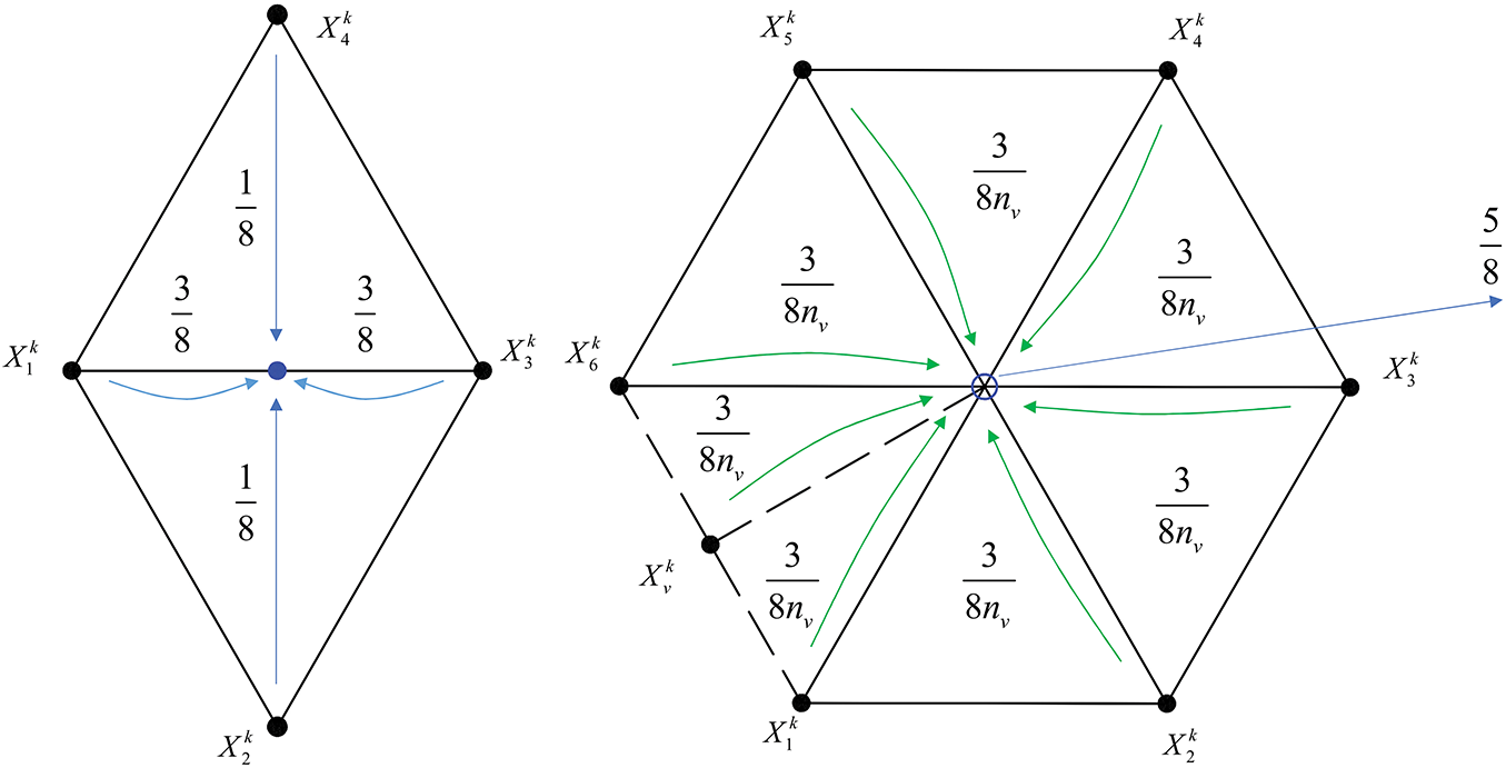
Figure 3: Refinement in loop subdivision

The vertex positions at level k+1 are computed as follows:

xek+1=18x1+38x2+18x3+38x4,(1)

xvk+1=38nv∑i=1vxi+58xvk.(2)

A key advantage of subdivision surfaces is their data-efficient representation, requiring only a compact initial mesh. While the number of irregular vertices (those with valence ≠6) may vary across elements in the original triangular mesh, a single iteration of the Loop subdivision scheme ensures that each refined triangular element contains exactly one irregular vertex, significantly simplifying topological complexity.

Analysis of Surface Fitting

Successive subdivisions of the initial mesh produce a smooth limit surface. Within subdivided surfaces, a triangular element is defined as regular if all its vertices are regular (valence nv=6) [34] (see the red triangular element in Fig. 4). For a point xe with local coordinates (θ1,θ2) (θ1,θ2∈[0,1]) in the regular element, its global coordinates can be directly interpolated using the quartic box-spline basis functions Bi and the coordinates of the corresponding control points xi (i.e., the 12 surrounding vertices):

xe(θ1,θ2)=∑i=112Bi(θ1,θ2)xi.(3)

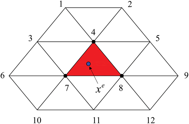
Figure 4: Control mesh vertices of a regular triangular element

For regular elements, Stam [35] defines the explicit form of these basis functions, which form the foundation for subdivision surface parameterization (Eq. (3)).

B1=112(θ14+2θ13θ2),B2=112(θ14+2θ13θ3),B3=112(θ14+2θ13θ3+6θ13θ2+6θ12θ2θ3+12θ12θ22+6θ1θ22θ3+6θ1θ23+2θ23θ3+θ24),B4=112(6θ14+24θ13θ3+24θ12θ32+8θ1θ33+θ34+24θ13θ2+60θ12θ2θ3+36θ1θ2θ32+6θ2θ33+ 24θ12θ22+36θ1θ22θ3+12θ22θ32+8θ1θ23+60θ23θ3+θ24),B5=112(θ14+6θ13θ3+12θ12θ32+6θ1θ33+θ34+2θ13θ2+6θ12θ2θ3+6θ1θ2θ32+2θ2θ33),B6=112(2θ1θ23+θ24),B7=112(θ14+6θ1θ33+12θ12θ32+6θ1θ33+θ34+8θ1θ2+36θ12θ2θ3+36θ1θ2θ32+8θ2θ33+24θ12θ22+ 60θ1θ22θ3+24θ22θ32+24θ1θ23+24θ23θ3+6θ24).(4)

For irregular elements consist of irregular vertices (nv≠6), the direct interpolation for points in regular elements is no longer applicable. To this end, a feature-based subdivision matrix method is adopted, whereby the irregular element is iteratively refined until the fitting point is relocated into a regular sub-element. Fig. 5 illustrates this process for a red triangular element containing vertex 1 (nv≠6), which is subdivided into three regular sub-elements (Γ11,Γ21 and Γ31) and one irregular sub-element. If the fitting point xe falls into one of the three regular sub-elements, then its parametric coordinates can be computed using the direct interpolation (see Eq. (3)). If xe falls into the irregular sub-element, this sub-element will be subdivided iteratively until xe locates in a regular sub-element. Detailed numerical implementation of the subdivision matrix method can refer to reference [35], Hence, the point in the irregular element can also be interpolated as:

xe(θ1,θ2)=∑i=1nv+6Ni(θ~1,θ~2)xi,(5)

which uses nv+6 control points, and the local coordinates in sub-elements (θ~1,θ~2)=(θ1,θ2)/2l, and l denotes the level of subdivision. More details can refer to [36].

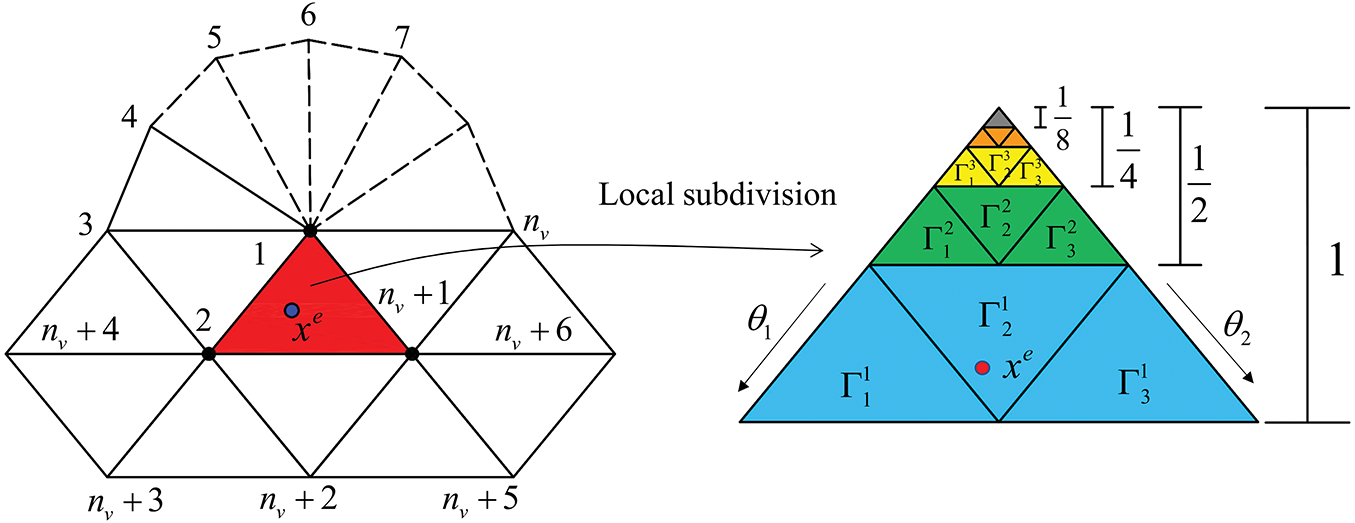
Figure 5: The control mesh vertices of irregular triangular elements in Loop subdivision surfaces

3  BEM for Acoustics

For acoustic scattering problems, the governing Helmholtz equation can be transformed into a conventional boundary integral [13].

c(x)p(x)−∫ΓG(x,y)q(y)dΓ(y)+∫Γp(y)∂G(x,y)∂n(y)dΓ(y)−pinc(x)=0,x∈Γ,(6)

where n(y) refers to the exterior normal direction, q(y)=∂p(y)∂n, the Green’s function G(x,y)=eikr4πr, and r denotes the distance between the source point x and field point y. pinc(x) represents the sound pressure caused by the incident wave, and Γ denotes the boundary of the structure. If the boundary is smooth, the coefficient c(x)=12. The total sound pressure p(x) is the summation of the incident sound pressure and the scattered sound pressure.

For acoustic problems, the boundary conditions are typically expressed as:

p(y)=p¯(y),y∈Γp,(7)

∂p∂n(y)=q¯(y),y∈Γq.(8)

where the boundary Γ is divided into boundary Γp with Dirichlet boundary condition and Γq with Neumann boundary conditions, i.e., Γ=Γp+Γq.

During the meshing process, the boundary was discretized and can be expressed as:

Γ=∑e=1NelΓe,(9)

where e denotes boundary element, and Nel is the total number of elements. For a field point y in the reference element with local coordinates (θ1,θ2), the acoustic pressure p(y) and its normal derivative q(y) can be expressed as:

p(y)=∑k=1NvNk(θ1,θ2)pk,q(y)=∑k=1NvNk(θ1,θ2)∂pk∂n.(10)

where Nv represents the number of basis functions Nk for a fitted boundary element with both regular and irregular elements (see Figs. 4 and 5, respectively), while k denotes the local index within the element patch.

Hence, the boundary integral Eq. (6) can be discretized as:

c(x)p(x)=∑e=1Nel∑k=1NvNk(θ1,θ2)∫Γe[G(x,y)∂pke∂n−∂G(x,y)∂n(y)pke]dΓe(y)+pinc(x).(11)

After assembling the equations for all collocation points and expressing them in matrix form [31], one can obtain the following system of linear algebraic equations:

pinc=Kp−Nq.(12)

where p and q represent vectors of sound pressures and flux coefficients, respectively, pinc denotes the incident wave results at the collocation points, while the BEM coefficient matrices K and N are associated with the subdivision surface [37].

However, in numerical implementation, density and asymmetry of the coefficient matrices K and N result in an O(N2) complexity for a problem of N degrees of freedom. The Fast Multipole Method (FMM) [38] can significantly accelerate the computation of subdivision surface BEM [39,40] and reduce memory consumption. For wideband problems, FMBEM uses a partial wave expansion to obtain the solution in low-frequency range, and a plane wave expansion method incorporating rapid interpolation and filtering techniques for the solution in the high-frequency range.

To accelerate numerical computation of subdivision surface BEM, the FMM algorithm needs to generate eight higher level child boxes from the lower level parent computational box surrounding the boundary elements. This refinement process continues until the number of boundary elements within each box falls below a specified threshold, thereby determining the highest subdivision level in the broadband FMBEM. During the construction of the tree structure, the total boundary integral is decomposed into two parts, i.e., the near-field and far-field as shown in Fig. 6. When the distance between x and y is relatively small, the coefficient matrix Cnear (where C represents either K or N) is calculated using the BEM, otherwise the far-field component Cfar is computed using the FMM.

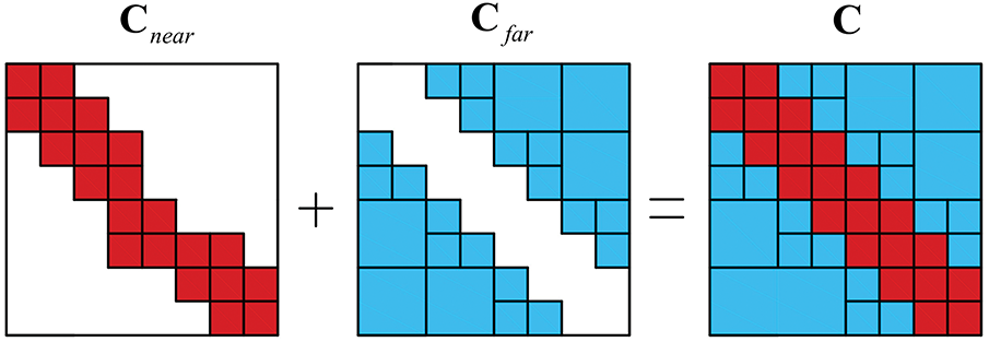
Figure 6: The coefficient matrix of the boundary element method is decomposed into two parts: the near-field and the far-field. Here, C=K,N

The kernel function expansion, based on the Gegenbauer addition theorem, can be written as:

{G(x,y)=ik4π∑n=0∞∑m=−nn(2n+1)I¯nm(k,ycy→)Onm(k,ycx→),|ycx→|>|ycy→|,G(x,y)=ik4π∑n=0∞∑m=−nn(2n+1)I¯nm(k,xcx→)Onm(k,xcy→),|xcy→|>|xcx→|,(13)

where yc and xc represent points near y and x, respectively. The term I¯nm denotes the complex conjugate of Inm, with the coefficients Inm and Onm defined as:

Inm(k,v→)=jn(kr)Ynm(θ,ϕ),(14)

Onm(k,v→)=hn(1)(kr)Ynm(θ,ϕ),(15)

where (r,θ,ϕ) represent the spherical coordinates of vector v→, jn is the Bessel function of the n-th order, hn(1) is the Hankel function of the first kind, and γnm is the spherical harmonic.

Partial derivative of the expanded kernel function with respect to the normal vector n can then be written as:

∂G(x,y)∂n(y)≈ik4π∑n=0∞∑m=−nn(2n+1) Onm(k,ycx→)∂I¯nm(k,ycy→)∂n(y).(16)

By using Eqs. (13) and (16), the boundary integral terms in the governing equation can be re-expressed as:

∫Γfar[∂G(x,y)∂n(y)∂n(y)p(y)−G(x,y)q(y)]dΓ(y)≈ik4π∑n=0∞∑m=−nn(2n+1)Onm(k,ycx→)Mnm(k,yc).(17)

In this context, Γfar represents the region Cfar illustrated in Fig. 6. The multipole expansion coefficient Mnm is expressed as:

Mnm(k,yc)=∫Γfar[∂I¯nm(k,ycy→)∂n(y)p(y)−I¯nm(k,ycy→)q(y)]dΓ(y).(18)

For more details of the FMM algorithm, please refer to [41,42].

4  CGAN for Accelerated Computation

Although FMM can greatly accelerate the computation of acoustic problems using subdivision surface BEM, the computational cost of large-scale and highly complex models is still unmanageable. To this end, neural networks have been extensively investigated in terms of accelerating computation of acoustic problems.

Typically, neural networks require a large number of training samples to achieve high prediction accuracy. However, obtaining such data is often complex, time-consuming, and computationally expensive. To address this limitation, this study employs a Conditional Generative Adversarial Network (CGAN) [43,44], which is capable of maintaining high prediction accuracy even with limited training data. The study first generates sample data through numerical simulations and uses this data as the training and testing dataset. The dataset was split into training and testing sets with a ratio of 9:1. Section 4.1 introduces the CGAN model and its numerical implementation.

CGAN Model

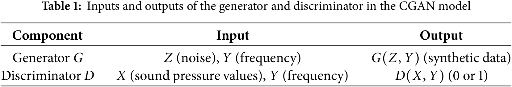
As shown in Fig. 7, the Conditional Generative Adversarial Network (CGAN) [45] comprises two adversarial neural networks: a generator that produces synthetic data and a discriminator that differentiates between real and generated data. In this study, the generator G receives random noise Z (a vector of random values between 0 and 1) and conditional input Y (representing frequency, e.g., 100 Hz) as input data, and produces (i.e., outputs) synthetic data G(Z,Y) that mimics the statistical distribution of real data. By integrating the conditional information Y, the model shifts from an unsupervised to a supervised learning paradigm, which facilitates precise control over the generated outputs.

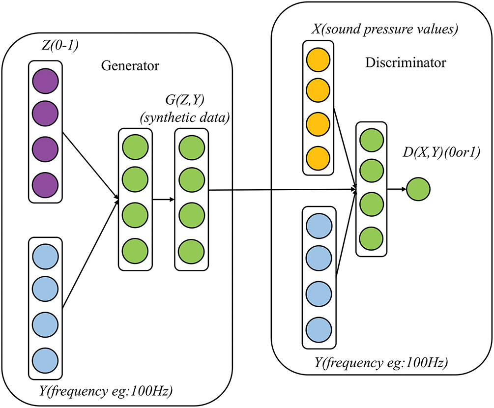
Figure 7: CGAN’s network structure

The discriminator D distinguishes real data from synthetic data, and thus its inputs include the real sound pressure data X (sound pressure values) with its corresponding condition Y (frequency), and the generated data G(Z,Y) paired with the same condition Y, while its output will be a binary value (0 or 1) denoting whether the data is real or synthetic data. During training, the generator and discriminator engage in an adversarial process, iteratively improving their performance. This dynamic resembles a minimax game, where both networks progressively converge toward a Nash equilibrium. At this equilibrium, the generator produces data indistinguishable from real data, and the discriminator cannot reliably differentiate between the two. Finally, the Table 1 presents the input and output structure of the CGAN model. In the CGAN model, the generator takes as input the random noise Z and the conditional information Y (i.e., frequency), and outputs G(Z,Y), which represents the generated data that follows the same pattern and distribution as the sound pressure. The discriminator receives the real sound pressure data X along with the corresponding condition Y, and outputs a binary result (0 or 1) indicating whether the input data is real or generated. Table 1 presents the input and output structure of the CGAN model.

Eq. (19) defines the CGAN’s adversarial objective function, which incorporates conditional information to establish a minimax optimization framework:

minGmaxDV(D,G)=EX∼Preal(X)[log⁡D(X,Y)]+EZ∼PZ(Z)[log⁡(1−D(G(Z,Y),Y))].(19)

Here, V denotes the value function of the adversarial game, and E represents the expectation operator. D(X,Y) corresponds to the discriminator’s output probability when evaluating real data X paired with its associated condition Y. Preal(⋅) and PZ(⋅) denote the probability distributions of the real data and latent noise, respectively. D(G(Z,Y),Y) reflects the discriminator’s evaluation of the generator’s synthetic output G(Z,Y) taking into consideration the conditional input Y.

In this architecture, the discriminator D operates as a binary classifier tasked with distinguishing real data from synthetic samples, whereas the generator G aims to synthesize data that matches the statistical distribution of the real data Preal(⋅). By explicitly conditioning both networks on Y, CGAN addresses the inherent limitations of traditional Generative Adversarial Networks (GANs), such as uncontrolled generation, and enables targeted synthesis of outputs aligned with specific frequency-based constraints.

During adversarial optimization, the generator G and the discriminator D iteratively refine their performance until reaching an equilibrium state where the discriminator cannot reliably differentiate between real and synthetic data. The training alternates between updating G and D, with the global loss function L(D,G) unifying their individual objectives:

L(D,G)=EX,Y∼Preal(X,Y)[log⁡D(X,Y)]+EY∼PY(Y),Z∼pZ(Z)[log⁡(1−D(G(Z,Y),Y))],(20)

while the loss functions for D and G can be expressed as:

LD=−E(X,Y)∼Preal(X,Y)[log⁡D(X,Y)]−EZ∼PZ(Z),Y∼PY(Y)[log⁡(1−D(G(Z,Y),Y))]LG=EZ∼PZ(Z),Y∼PY(Y)[log⁡(1−D(G(Z,Y),Y))].(21)

Notably, CGAN’s generator inherently produces diverse synthetic datasets by sampling from Preal(⋅) and PZ(⋅). These generated samples further refine the discriminator’s accuracy during training, creating a mutually reinforcing cycle. This capability enables CGAN to address the challenges outlined in this study, such as generating targeted outputs under conditional constraints while maintaining data diversity.

5  Numerical Examples

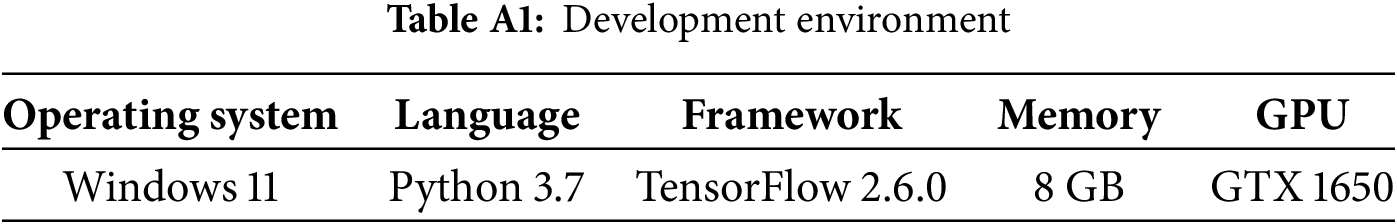
In this study, the isogeometric analysis method described in Section 3 was implemented using custom Fortran 90 code, while the CGAN framework outlined in Section 4 was developed in Python. All simulations were performed on a laptop with an Intel Core i5 processor and 8 GB of RAM. All models in this study use structural steel as the material, with a density of 7.86×103kg/m3, a Young’s modulus of 2.10×1011Pa, and a Poisson’s ratio of 0.30. Numerical examples were conducted to validate the efficiency and accuracy of the proposed CGAN-based accelerated computational method. The workflow for these numerical experiments is illustrated in Fig. 8.

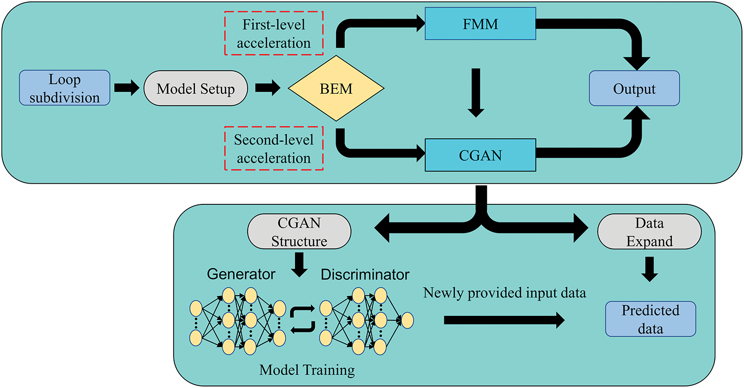
Figure 8: CGAN workflow for accelerating three-dimensional acoustic analysis

5.1 Spherical Model

We employ the boundary element method based on subdivision surfaces to analyze a spherical object with a radius of 1.2 m subjected to a unit-amplitude plane wave incident along the x-axis, the wave number is 0.100. The observation point is located at the coordinates (3, 0, 0 m), and additional geometric details are illustrated in Fig. 9. As a canonical three-dimensional acoustic problem [46], this spherical model has an analytical solution, making it a reliable benchmark for evaluating the accuracy and efficiency of the proposed algorithm.

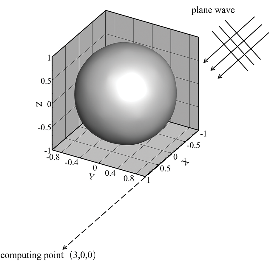
Figure 9: Acoustic scattering of a spherical model

The spherical mesh was refined iteratively using the Loop subdivision surface method (Fig. 10). Starting from a coarse polyhedral mesh, successive subdivision steps generated progressively smoother surfaces. Thus, it can bring higher computational accuracy.

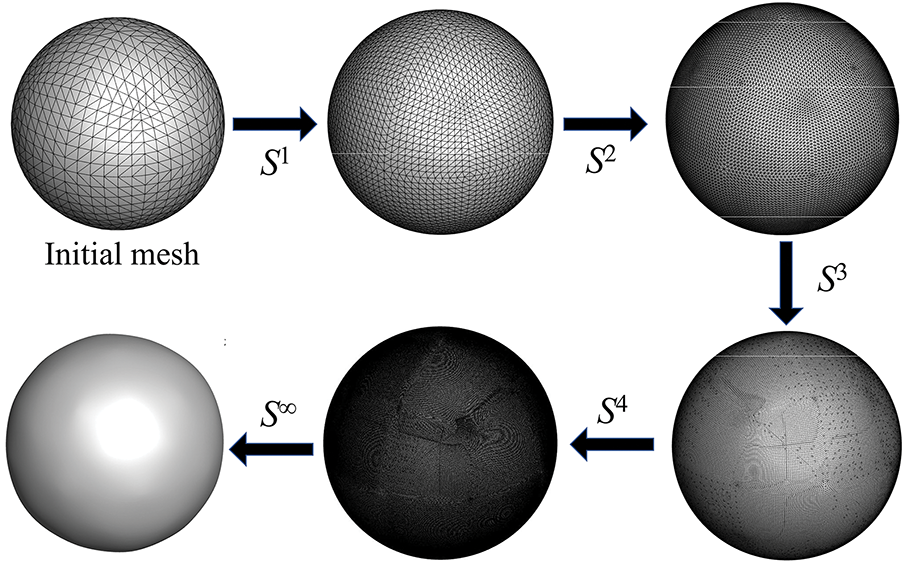
Figure 10: Sphere model meshes at different levels of subdivision

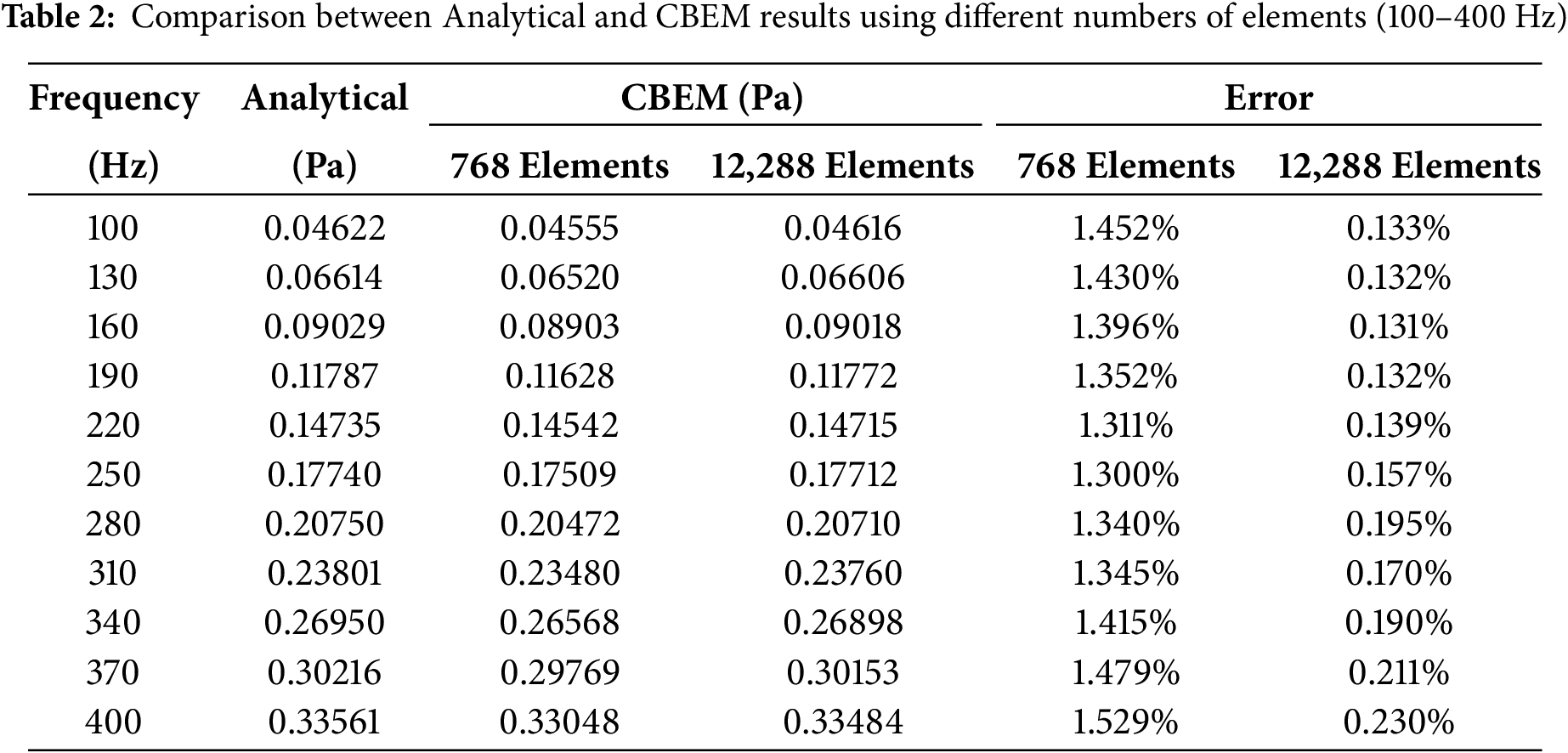
The Table 2 presents the errors between the numerical solutions obtained by the Boundary Element Method (BEM) and the analytical solutions for the spherical model with an initial mesh of 768 elements after two successive refinements. It can be observed that the refined mesh obtained through subdivision exhibits significantly smaller errors between the numerical and analytical solutions in the low-frequency range compared to the coarse mesh, resulting in an overall improvement in computational accuracy relative to the unrefined mesh. The spherical model in the example is based on an initial mesh of 768 elements, refined two times.

The discretized spherical model was solved via the Boundary Element Method (BEM), and a CGAN model was then trained to predict acoustic responses. To validate the proposed method’s correctness, an initial dataset generated by BEM calculations was divided into training and testing sets, with the CGAN training process detailed in Appendix A. After training, the model’s accuracy was evaluated on the test set, as shown in Figs. 11 and 12.

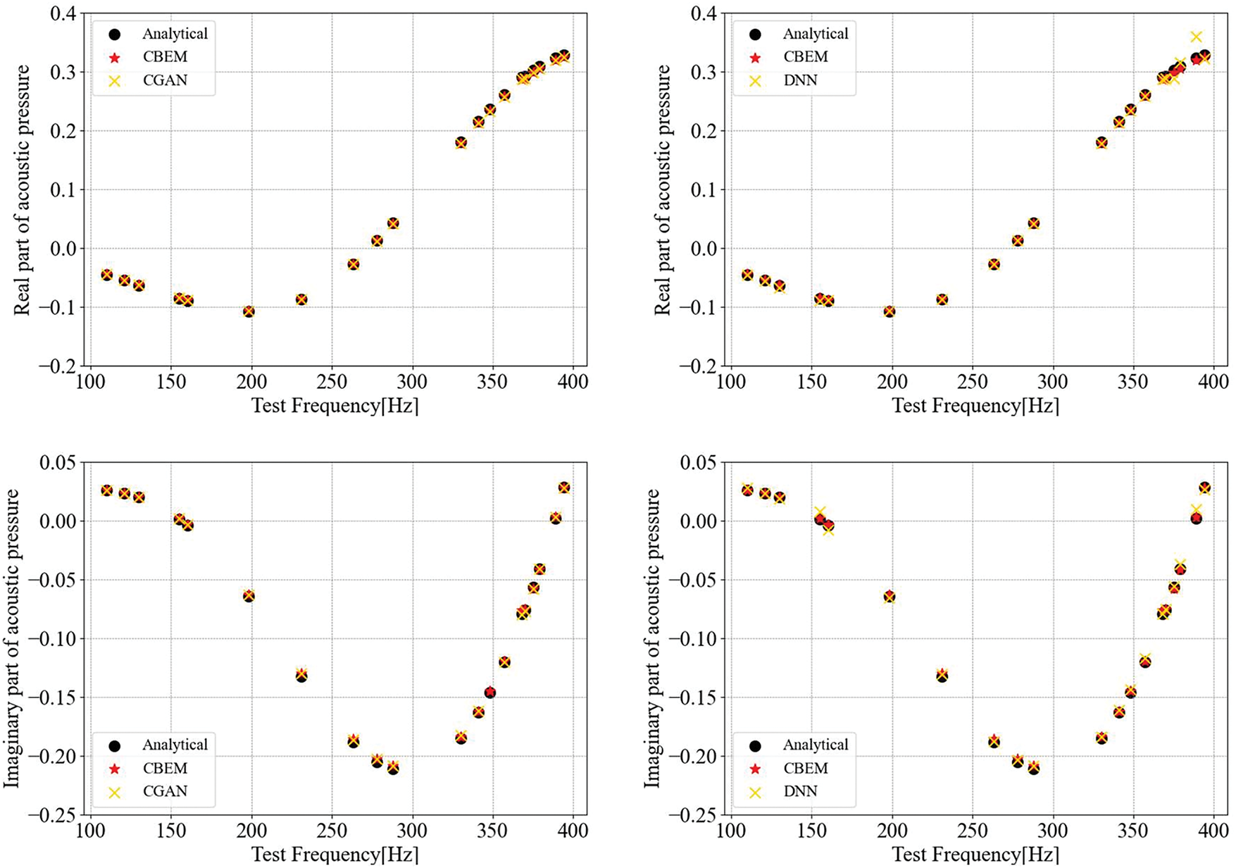
Figure 11: Real and imaginary parts of the acoustic pressure at point (3, 0, 0) obtained using different methods based on the subdivision surface

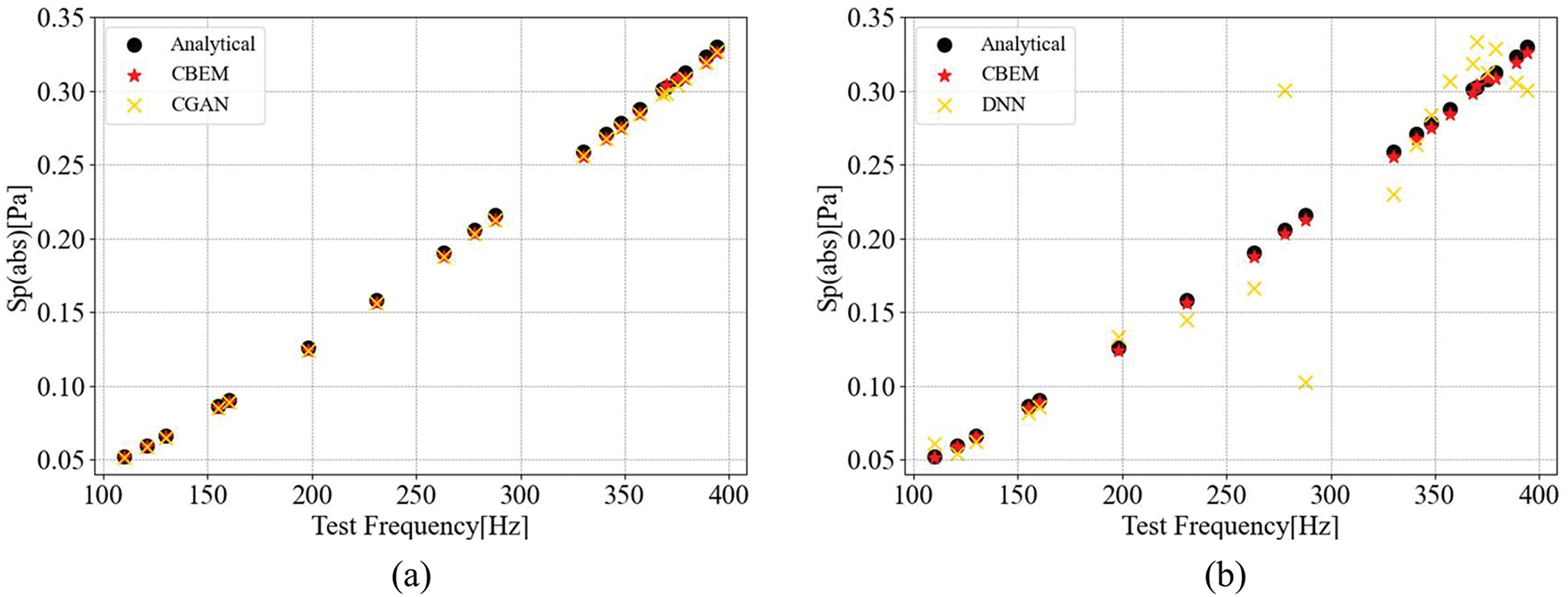
Figure 12: Sound pressure at point (3, 0, 0) obtained using different methods based on the subdivision surface: Comparison between results obtained from analytical solution, CBEM and (a) CGAN predictions; (b) DNN predictions

Fig. 11 compares the real and imaginary components of the acoustic pressure predicted by CGAN, DNN, and conventional models, while Fig. 12 illustrates their performance in predicting sound pressure magnitude. The CGAN model outperforms other methods in capturing both the complex components and overall pressure trends. By incorporating generator-synthesized data during training, CGAN maintains high accuracy even at dataset boundaries (100 and 400 Hz), where DNNs [47–49] struggle due to sparse boundary data. Notably, CGAN predictions align closely with analytical solutions, achieving accuracy comparable to the conventional BEM (CBEM).

The subdivision surface method enhances computational accuracy by iteratively refining meshes. However, this refinement significantly increases mesh density, leading to higher computational costs and prolonged simulation times. Consequently, traditional boundary element methods (BEM) struggle to efficiently handle complex models with fine meshes due to these scalability limitations. To mitigate this trade-off, the CGAN model was introduced to augment sparse datasets and accelerate computations.

To do this, the conventional boundary element method (CBEM) first computed sound pressure values at the observation point (3, 0, 0) across the 100–400 Hz frequency range using coarse 10 Hz intervals. This sparse dataset served as the training input for the CGAN model. After training, the CGAN generated predictions at a refined 1 Hz resolution, effectively augmenting the dataset. The augmented results were then rigorously validated against both CBEM outputs and analytical solutions, as demonstrated in Figs. 13 and 14, confirming the method’s ability to balance accuracy and efficiency.

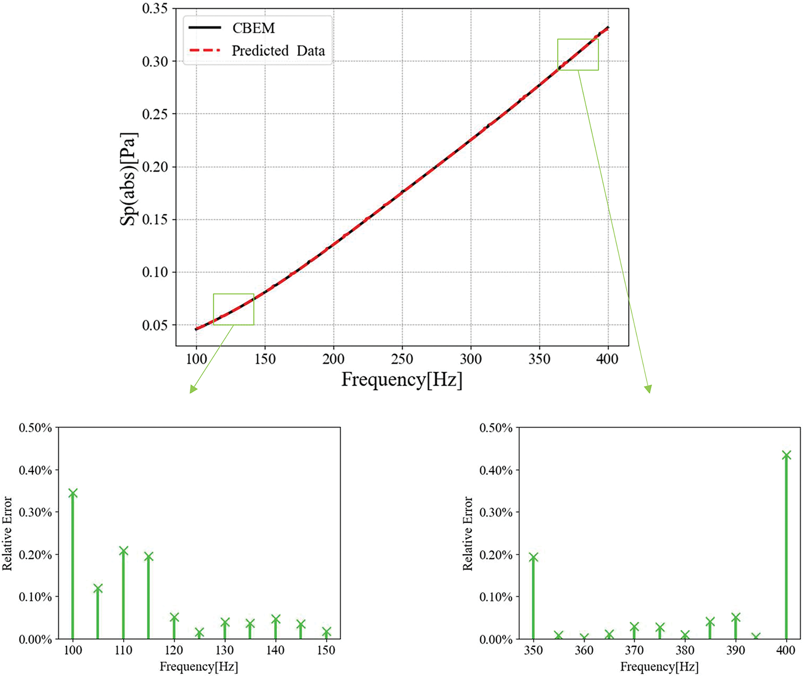
Figure 13: Comparison of CGAN-augmented data and CBEM results

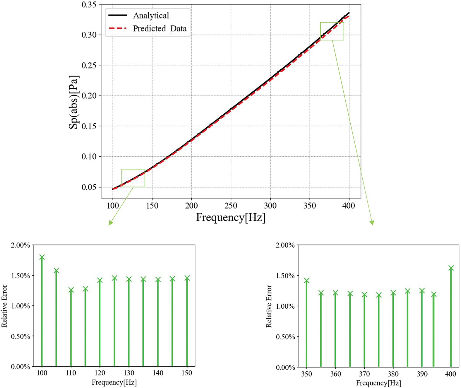
Figure 14: Comparison of CGAN-augmented data and analytical solutions

The CGAN-augmented data shows a high degree of agreement with both the analytical solution and the CBEM results, confirming that the model successfully learned the underlying data patterns and generalized effectively to unseen frequencies. As shown in the subfigure, relative errors at the dataset boundaries (100 nd 400 Hz) with respect to both algorithms are less than 2%. Specifically, the Fig. 14 demonstrates that CGAN and CBEM achieve nearly identical accuracy, as the errors are very small. These findings validate CGAN as an effective tool for accelerating computations without sacrificing precision. Furthermore, comparison with CBEM results reveals that CGAN achieves comparable predictive accuracy while significantly reducing computational effort, establishing its dual advantage in both accuracy and efficiency for acoustic analysis.

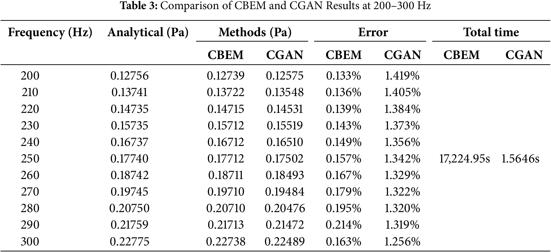
Table 3 provides a validation of the CGAN model’s predictive accuracy in the mid-frequency range, confirming that CGAN and CBEM achieve statistically indistinguishable error levels relative to analytical solutions, with discrepancies below 0.5% in mid-range frequencies. However, CGAN reduces computational time by orders of magnitude compared to CBEM when processing equivalent datasets. Typically, training a well-performing CGAN model takes about 30 min, while generating the initial dataset through numerical simulation with a frequency step of 10 Hz requires approximately 35 min. Overall, compared to computing all frequency points, this approach reduces computational costs. However, in practical applications, it is usually unnecessary to calculate the sound pressure at every frequency point. This condition is set here mainly to verify that CGAN can effectively assist computations in certain specific cases.

From this example, it can be observed that the subdivision surface method further enhances computational accuracy by generating smooth, high-quality meshes through iterative refinement of coarse polyhedral models. This approach produces multi-resolution meshes capable of handling complex geometries while improving numerical integration accuracy—a critical factor for precise boundary element calculations. Its adaptability to intricate structures, coupled with widespread software integration, makes it indispensable for 3D acoustic problems requiring geometric fidelity. However, finer meshes increase computational costs, exacerbating the trade-off between accuracy and efficiency.

This challenge is mitigated by the CGAN model, which uniquely addresses data scarcity inherent to high-fidelity 3D acoustic modeling. Conventional neural networks struggle in such scenarios due to the prohibitive computational cost of generating large training datasets. CGAN circumvents this limitation by leveraging conditional information (e.g., frequency) to synthesize physically realistic data through its adversarial framework. The generator produces virtual data distributions that mimic real data, while the discriminator refines its validation criteria iteratively. This process enables robust training on sparse datasets, achieving accuracy rivaling CBEM with far less computational overhead. By integrating subdivision surfaces for computational accuracy and CGAN for data-efficient acceleration, the proposed framework offers a balanced solution to the accuracy-efficiency trade-off in 3D acoustic analysis.

5.2 Washing Machine Model

To validate the generalizability of the CGAN framework across complex geometries and diverse acoustic scenarios, we analyzed a washing machine model in this section. The observation point was positioned at (0.5, 0, 0 m), with geometric and boundary condition details illustrated in Fig. 15. First, we considered a unit-amplitude plane wave incident along the positive x-axis, analogous to the spherical model case.

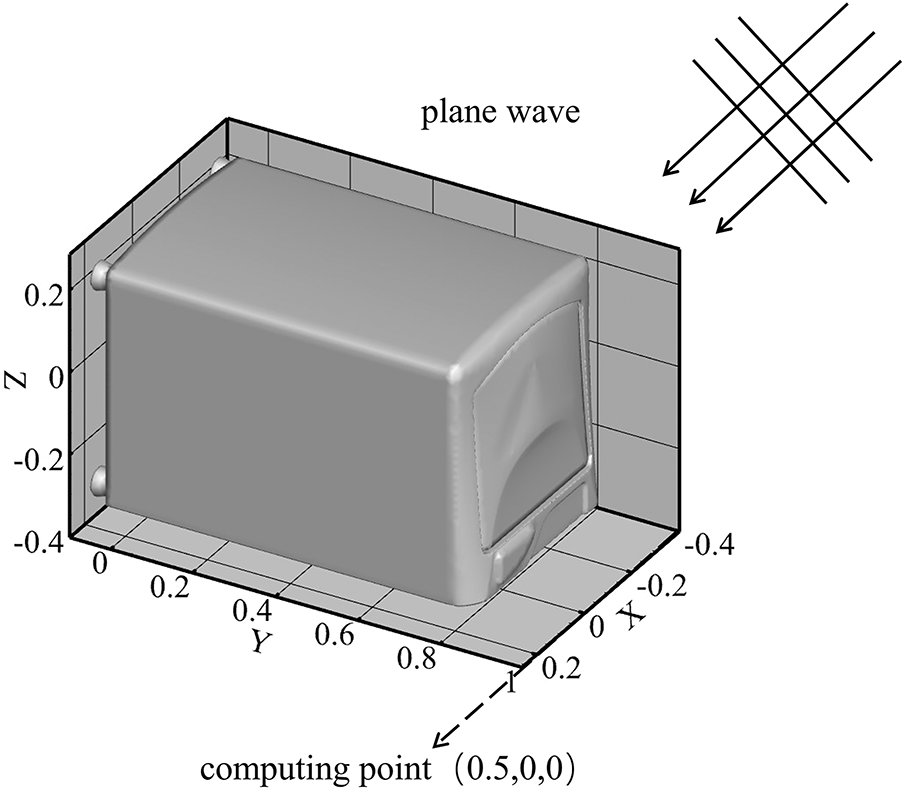
Figure 15: Acoustic scattering of a washing machine model

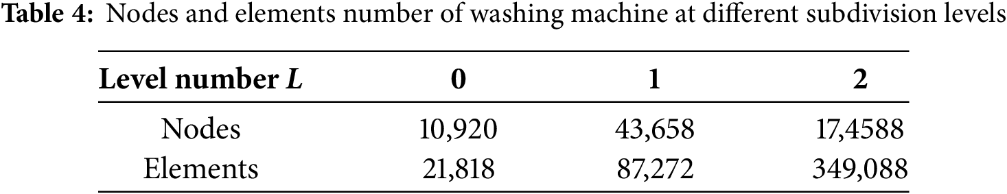
The model was discretized using Loop subdivision surfaces, with mesh refinement levels shown in Fig. 16 and quantified in Table 4. Each subdivision level quadruples the number of nodes and elements, progressively approximating the ideal subdivided surface. However, higher subdivision levels impose prohibitive computational and memory demands, rendering BEM calculations impractical. To balance accuracy and resource constraints, we selected the Level 1 mesh (43,658 nodes, 87,272 elements) for subsequent analyses.

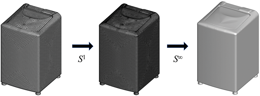
Figure 16: Meshes of washing machine model at different levels of subdivision

BEM simulations for the washing machine model proved computationally prohibitive, with even sparse initial datasets requiring substantial calculation time. To address this, we implemented a two-stage acceleration strategy. First, the fast multipole method (FMM) was integrated with the Loop subdivision surface technique to create an accelerated BEM framework (FMBEM) for efficient initial data generation.

The accuracy of this FMBEM implementation was validated by comparing real and imaginary sound pressure components at the observation point against conventional BEM results, as illustrated in Fig. 17. The near-identical agreement confirms that FMBEM preserves BEM’s precision while drastically reducing computation time. This validated FMBEM served as the foundation for generating training data.

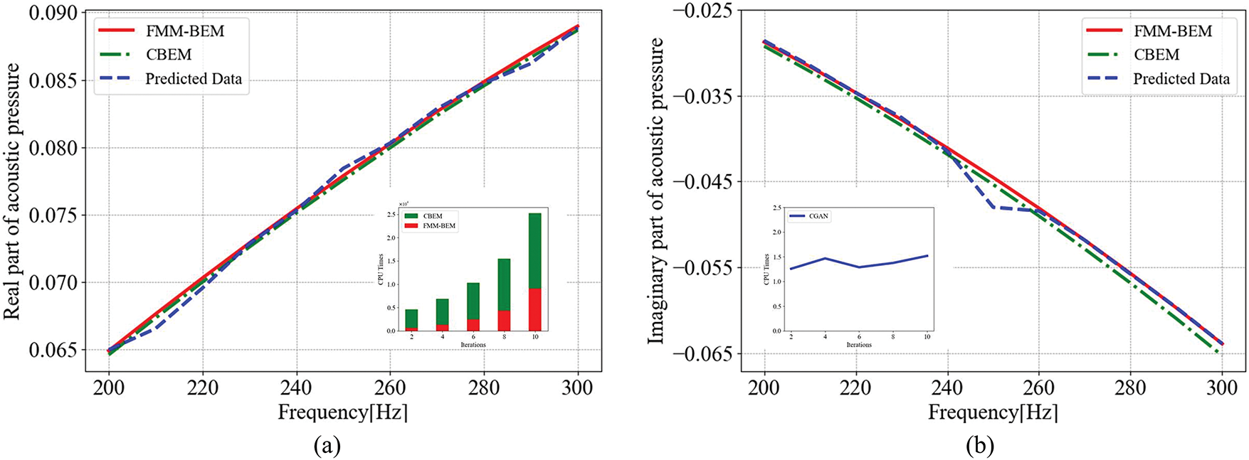
Figure 17: The acoustic pressure at point (0.5, 0, 0) using different methods based on the subdivision surface: (a) Real part and (b) Imaginary part of the aoustic pressure

Subsequently, the CGAN model was deployed as a secondary acceleration stage. Leveraging the FMBEM-computed dataset, CGAN performed data augmentation to predict high-resolution frequency responses, further accelerating the workflow without compromising accuracy. This hybrid approach—combining FMBEM for initial acceleration and CGAN for predictive augmentation—effectively addresses the computational bottlenecks of complex acoustic simulations.

The predicted results in Fig. 17 were generated after validating the accuracy of the fast multipole algorithm. Training data were computed at 20 Hz intervals in (200–300 Hz) using the fast multipole boundary element method (FMBEM). The trained CGAN model then augmented this dataset to a finer 10 Hz resolution, and the predictions were compared with numerical solutions. The results show close agreement between the CGAN-augmented data and numerical benchmarks, with only minor deviations at specific frequencies.

The subfigures in Fig. 17 also compare the computational time required for calculating 10 data points using the boundary element method (BEM), fast multipole method (FMM), and CGAN. The FMM significantly reduces computation time compared to conventional BEM. During BEM simulations, real and imaginary components are computed simultaneously, whereas the CGAN model bypasses this complexity by learning data patterns directly. As shown in the right subfigure, CGAN generates large datasets rapidly, with computation time remaining nearly constant regardless of data volume. This efficiency confirms CGAN’s ability to accelerate computations without compromising accuracy.

The sound pressure distribution across the model surface was analyzed at four distinct frequencies, as shown in Fig. 18. At lower frequencies (100–200 Hz), the surface pressure distribution exhibits minimal variation. In contrast, at higher frequencies (400–600 Hz), significant changes occur, particularly on the washing machine’s outer surface where incident wave energy concentrates. These variations grow increasingly pronounced with rising frequency, highlighting the dynamic response of the structure under acoustic excitation.

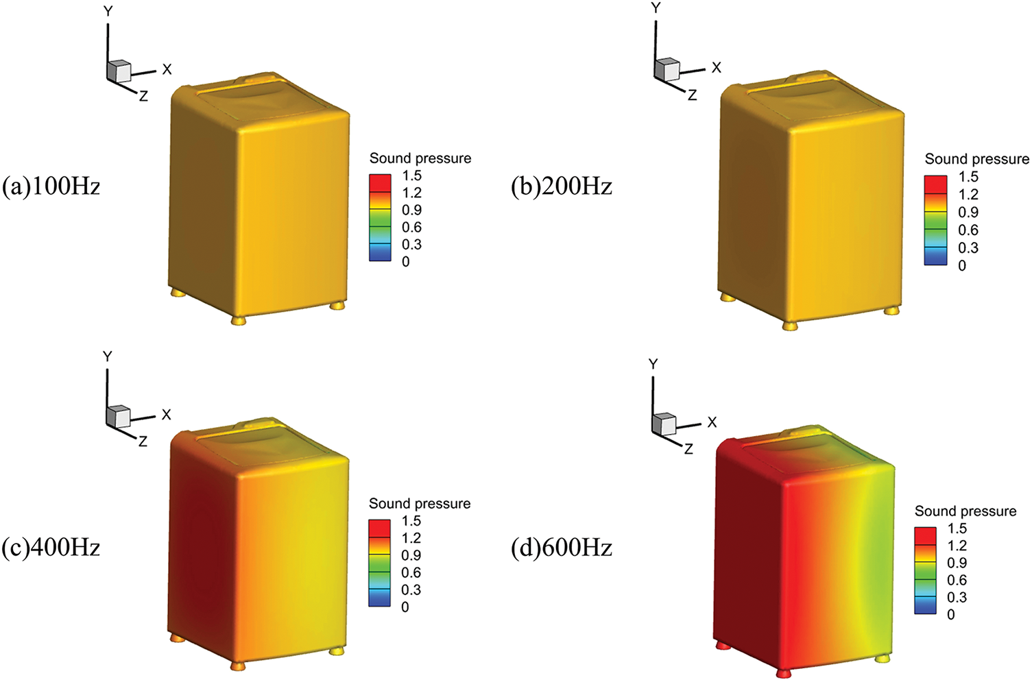
Figure 18: Sound pressure contour on the surface of the washing machine at different frequencies: (a) Frequency = 100 Hz; (b) Frequency = 200 Hz; (c) Frequency = 400 Hz; (d) Frequency = 600 Hz

5.3 Vibration Issues in the Washing Machine Model

Results of this study can help address a critical engineering challenge: understanding how vibrations generated during washing machine operation influence acoustic phenomena. These vibrations, an inevitable result of mechanical activity, often produce complex noise patterns. To investigate this interaction, vibrations were systematically applied to the washing machine model, and their effects on sound pressure distribution and acoustic performance were analyzed. The findings aim to advance theoretical insights and practical strategies for mitigating vibration-induced noise in industrial applications.

This study evaluates the CGAN model’s applicability to vibration acoustics by treating the washing machine as a rigid structure. The primary objective is to assess CGAN’s capability in predicting vibration-dependent sound pressure distributions. To quantify noise impacts under realistic conditions, two operational scenarios were simulated: Case 1 represents an observation point located at (0.5, 0, 1), while Case 2 represents an observation point at (0.5, 0, 1.8). These cases represent noise exposure at distinct heights, mimicking human ear levels in different positions. Corresponding CGAN predictions (labeled Case x-CGAN) are illustrated in Fig. 19, demonstrating the model’s ability to map vibration patterns to acoustic responses.

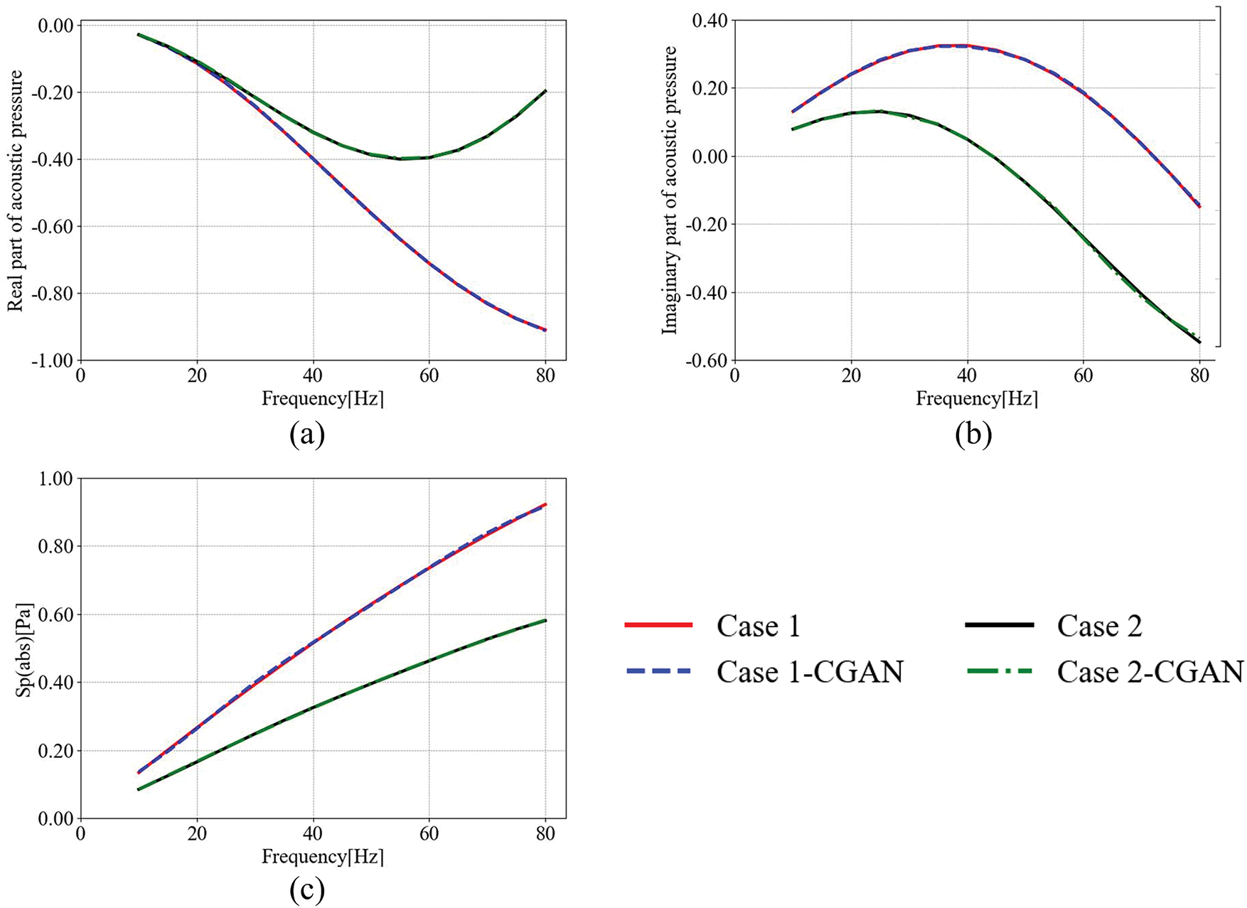
Figure 19: The acoustic pressure at computation points (0.5, 0, 1) and (0.5, 0, 1.8) obtained using the subdivision surface: (a) Real part; (b) Imaginary part; (c) Total sound pressure

The results in Fig. 20 reveal distinct trends in acoustic pressure characteristics at the two observation points. Case 1 (0.5, 0, 1) exhibits markedly higher magnitudes in the real part, imaginary part, and total sound pressure compared to Case 2 (0.5, 0, 1.8). Furthermore, the acoustic pressure in Case 1 increases more sharply with frequency, suggesting that lower positions experience greater noise exposure.

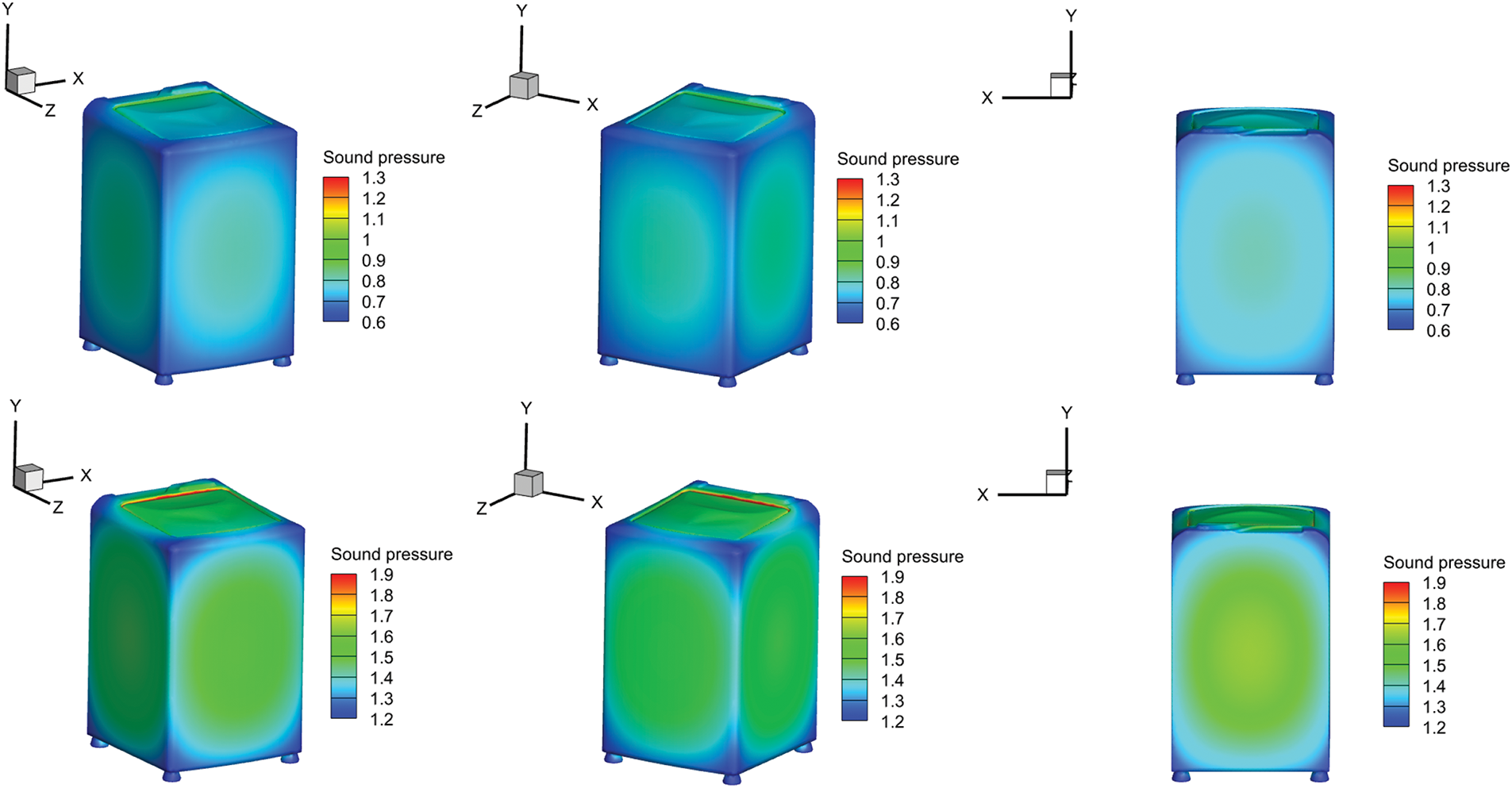
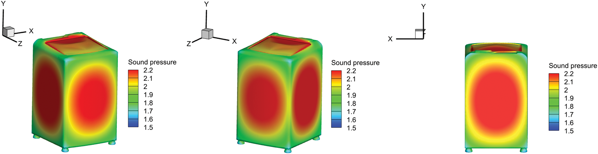
Figure 20: Sound pressure contour on the surface of the washing machine at different frequencies

The CGAN model achieves excellent agreement with reference data in predicting both complex components (real/imaginary) and total sound pressure, validating its ability to learn vibration-acoustic correlations and deliver high-fidelity predictions. This underscores CGAN’s key strength: its capacity to uncover latent data patterns irrespective of problem complexity, enabling reliable generalization across diverse scenarios.

In addition to localized noise analysis, Fig. 20 illustrates the spatial sound pressure distribution across the washing machine surface, further demonstrating the interplay between structural vibrations and acoustic responses.

6  Conclusion

A novel acceleration algorithm is proposed based on the loop subdivision surface method for BEM computation of acoustic scattering problems. This algorithm first accelerates computations using the fast multipole boundary element method (FMBEM) and then achieves secondary acceleration through data augmentation with the CGAN model. The accuracy of the BEM and CGAN model was validated using the spherical model example, confirming their high precision. The FMBEM’s accuracy was further verified with the washing machine model, demonstrating that the CGAN model retains high precision even for complex geometries. Practical engineering applications validated the algorithm’s effectiveness for real-world problems. The proposed secondary acceleration algorithm offers three key advantages:

1.   Smoother geometric models generated via Loop subdivision surfaces, ensuring high-precision computational inputs.

2.   Higher computational efficiency than traditional methods while maintaining accuracy.

3.   Broad applicability to diverse acoustic problems.

The limitations of the method are as follows: if the initial mesh quality is poor, it may compromise the smoothness of the subdivided geometry and the accuracy of the BEM discretization, thereby limiting the method’s applicability to complex geometries. Moreover, for highly complex models, the training time of the CGAN increases significantly, which may diminish the efficiency advantage of the proposed algorithm.

Future work will focus on applying this algorithm to three-dimensional acoustic sensitivity analysis and noise reduction optimization in practical engineering scenarios, through shape optimization or the application of adhesive sound-absorbing materials. In addition, the integration of Bayesian Neural Networks (BNNs) will be considered for uncertainty quantification, aiming to investigate the influence of material properties and other factors on sensitivity.

Acknowledgement: The authors would like to express their sincere thanks to Dr. Leilei Chen from Huanghuai University for his valuable suggestions in improving this manuscript.

Funding Statement: The author would like to thank the support from the 2025 Henan Provincial Science and Technology Research Project, the Zhumadian 2023 Major Science and Technology Special Project, and the Postgraduate Education Reform and Quality Improvement Project of Henan Province.

Author Contributions: The authors confirm contribution to the paper as follows: study conception and design: Ziyu Cui, Pei Li; data collection: Ziyu Cui; analysis and interpretation of results: Zijun Wei, Xiaohui Yuan, Pei Li; draft manuscript preparation: Ziyu Cui, Zijun Wei; manuscript revision: Xiaohui Yuan, Pei Li. All authors reviewed the results and approved the final version of the manuscript.

Availability of Data and Materials: The datasets generated and/or analyzed during the current study are available from the corresponding author on reasonable request.

Ethics Approval: Not applicable.

Conflicts of Interest: The authors declare no conflicts of interest to report regarding the present study.

Appendix A Arrangements for Network Training

The neural network training process requires careful selection of hyperparameters—such as learning rate, activation function, and optimizer—which critically influence model performance and training efficiency. To ensure network effectiveness and accuracy, hyperparameter tuning and optimization are essential. This appendix details the training of the CGAN model using spherical model data computed across the 100–400 Hz frequency range. This training workflow includes three key steps: data preprocessing, feature normalization, and network architecture design, all implemented to ensure training stability and convergence. The same procedure was applied to other models, enabling the CGAN network to generalize effectively across diverse acoustic analysis tasks while maintaining computational acceleration. A complete summary of hyperparameters and configurations is provided in Table A1.

For data preprocessing, the CGAN network employs min-max normalization (Eq. (A1)) to scale input features into a unified numerical range. This mitigates biases caused by varying data magnitudes and enhances training robustness.

x′=xinput−min(xinput)max(xinput)−min(xinput)(A1)

Here, xinput refers to the real data input into both the generator and the discriminator.

For regression-type acoustic problems, the loss function is defined as the Mean Squared Error (MSE), which quantifies the deviation between predicted and true values:

MSE=1N∑i=1N(yi−y^i)2(A2)

where yi and y^i represent the true and predicted values of the i-th sample, respectively.

After initializing key hyperparameters, the CGAN training process begins. The learning rate and number of hidden layers are iteratively optimized by monitoring loss convergence. The Sigmoid activation function is selected for both the discriminator and generator. For the discriminator, Sigmoid outputs a probability (0 or 1) to classify real vs. synthetic data. For the generator, Sigmoid ensures output consistency with the discriminator’s input format. Training outcomes, including loss dynamics and model performance, are illustrated in Fig. A1, demonstrating stable convergence and effective adversarial learning.

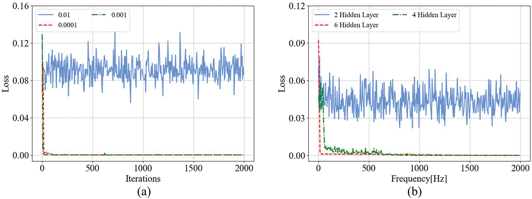
Figure A1: The CGAN training loss: (a) Learning rate; (b) Hidden layer

The results demonstrate that a learning rate of 0.0001 enables faster loss convergence with minimal oscillations compared to a rate of 0.001. Similarly, a network configuration with six hidden layers achieves rapid and stable loss convergence, outperforming other layer configurations. These findings underscore the importance of optimizing both learning rate and hidden layer count for enhancing model stability and performance. The finalized architecture and hyperparameters of the CGAN model are summarized in Table A2.

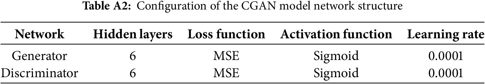
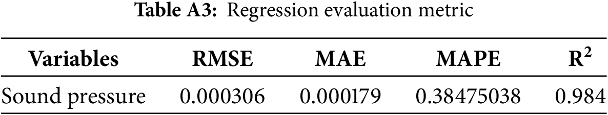
Table A3 provides multiple regression evaluation metrics, all satisfying predefined thresholds, collectively validating the model’s high accuracy. The consistent performance across metrics demonstrates the model’s ability to effectively capture data patterns and deliver reliable predictions.

For other examples in this study, the training follows the same workflow as the spherical model. To ensure CGAN accuracy, a dedicated model must be trained for each new geometry or data distribution.

References

1. Liu Z, Sheng L, Liu X, Chang Y, Chen G, Guo X. Mechanical analysis for deepwater drilling riser system with structural parameters uncertainty. Ocean Eng. 2024;305(3):118049. doi:10.1016/j.oceaneng.2024.117657. [Google Scholar] [CrossRef]

2. Mahrous E, Valéry Roy R, Jarauta A, Secanell M. A three-dimensional numerical model for the motion of liquid drops by the particle finite element method. Phys Fluids. 2022;34(5):052120. doi:10.1063/5.0091699. [Google Scholar] [CrossRef]

3. Vuong CD, Yu T, Rungamornrat J, Bui TQ. A smoothing gradient thermo-mechanical damage model for thermal shock crack propagation: theory and FE implementation. Int J Non Linear Mech. 2024;163(B12):104755. doi:10.1016/j.ijnonlinmec.2024.104755. [Google Scholar] [CrossRef]

4. Liu Z, Majeed M, Cirak F, Simpson RN. Isogeometric FEM-BEM coupled structural-acoustic analysis of shells using subdivision surfaces. Int J Num Meth Eng. 2018;113(9):1507–30. doi:10.1002/nme.5708. [Google Scholar] [CrossRef]

5. Pei Q, Li F, Fei Z, Lian H, Yuan X. A DFE2-SPCE method for multiscale parametric analysis of heterogenous piezoelectric materials and structures. Comput Mater Contin. 2025;83(1):79–96. doi:10.32604/cmc.2025.061741. [Google Scholar] [CrossRef]

6. Zheng CJ, Gao HF, Du L, Chen HB, Zhang C. An accurate and efficient acoustic eigensolver based on a fast multipole BEM and a contour integral method. J Computat Physics. 2016;305:677–99. doi:10.1016/j.jcp.2015.10.048. [Google Scholar] [CrossRef]

7. Marburg S, Nolte B. Computational acoustics of noise propagation in fluids: finite and boundary element methods. Vol. 578. Berlin, Germany: Springer; 2008. [Google Scholar]

8. Marburg S. The Burton and Miller method: unlocking another mystery of its coupling parameter. J Comput Acoust. 2016;24(1):1550016. doi:10.1142/s0218396x15500162. [Google Scholar] [CrossRef]

9. Huo R, Pei Q, Xu Y, Xu Y. Generalized nth-order perturbation method based on loop subdivision surface boundary element method for three-dimensional broadband structural acoustic uncertainty analysis. Comput Model Eng Sci. 2024;140(2):2053–77. doi:10.32604/cmes.2024.049185. [Google Scholar] [CrossRef]

10. Hughes TJ, Cottrell JA, Bazilevs Y. Isogeometric analysis: CAD, finite elements, NURBS, exact geometry and mesh refinement. Comput Methods Appl Mech Eng. 2005;194(39–41):4135–95. doi:10.1016/j.cma.2004.10.008. [Google Scholar] [CrossRef]

11. Bazilevs Y, Calo VM, Cottrell JA, Evans JA, Hughes TJR, Lipton S, et al. Isogeometric analysis using T-splines. Comput Methods Appl Mech Eng. 2010;199(5–8):229–63. doi:10.1016/j.cma.2009.02.036. [Google Scholar] [CrossRef]

12. Barendrecht PJ, Bartoň M, Kosinka J. Efficient quadrature rules for subdivision surfaces in isogeometric analysis. Comput Meth Appl Mech Eng. 2018;340:1–23 doi:10.1016/j.cma.2018.05.017. [Google Scholar] [CrossRef]

13. Chen L, Wang Z, Lian H, Ma Y, Meng Z, Li P, et al. Reduced order isogeometric boundary element methods for CAD-integrated shape optimization in electromagnetic scattering. Comput Methods Appl Mech Eng. 2024;419:116654 doi:10.1016/j.cma.2023.116654. [Google Scholar] [CrossRef]

14. Cervera E, Trevelyan J. Evolutionary structural optimisation based on boundary representation of NURBS. Part II: 3D algorithms. Comput Struct. 2005;83(23–24):1917–29 doi:10.1016/j.compstruc.2005.02.017. [Google Scholar] [CrossRef]

15. Burkhart D, Hamann B, Umlauf G. Iso-geometric finite element analysis based on catmull-clark: ubdivision solids. In: Computer graphics forum. Vol. 29. Hoboken, NJ, USA: Wiley Online Library; 2010. p. 1575–84. [Google Scholar]

16. Cirak F, Ortiz M, Schröder P. Subdivision surfaces: a new paradigm for thin-shell finite-element analysis. Int J Numer Metho Eng. 2000;47(12):2039–72 doi:10.1002/(sici)1097-0207(20000430)47:12<2039::aid-nme872>3.0.co;2-1. [Google Scholar] [CrossRef]

17. Dyn N, Levine D, Gregory JA. A butterfly subdivision scheme for surface interpolation with tension control. ACM Transact Graph. 1990;9(2):160–9 doi:10.1145/78956.78958. [Google Scholar] [CrossRef]

18. Bandara K, Cirak F, Of G, Steinbach O, Zapletal J. Boundary element based multiresolution shape optimisation in electrostatics. J Computat Phy. 2015;297:584–98. doi:10.1016/j.jcp.2015.05.017. [Google Scholar] [CrossRef]

19. Settgast V, Müller K, Fünfzig C, Fellner D. Adaptive tesselation of subdivision surfaces. Comput Graph. 2004;28(1):73–8. [Google Scholar]

20. Morin G, Warren J, Weimer H. A subdivision scheme for surfaces of revolution. Comput Aid Geomet Des. 2001;18(5):483–502. doi:10.1016/s0167-8396(01)00043-7. [Google Scholar] [CrossRef]

21. Cirak F, Long Q. Subdivision shells with exact boundary control and non-manifold geometry. Int J Numer Meth Eng. 2011;88(9):897–923. doi:10.1002/nme.3206. [Google Scholar] [CrossRef]

22. Chen L, Lian H, Liu C, Li Y, Natarajan S. Sensitivity analysis of transverse electric polarized electromagnetic scattering with isogeometric boundary elements accelerated by a fast multipole method. Appl Math Model. 2025;141(47):115956. doi:10.1016/j.apm.2025.115956. [Google Scholar] [CrossRef]

23. Marburg S, Schneider S. Performance of iterative solvers for acoustic problems. Part I. Solvers and effect of diagonal preconditioning. Eng Analy Bound Elem. 2003;27(7):727–50. doi:10.1016/s0955-7997(03)00025-0. [Google Scholar] [CrossRef]

24. Marburg S. Numerical damping in the acoustic boundary element method. Acta Acustica United with Acustica. 2016;102(3):415–8. [Google Scholar]

25. Fischer M, Gaul L. Application of the fast multipole BEM for structural–acoustic simulations. J Computat Acoust. 2005;13(1):87–98. doi:10.1142/s0218396x05002578. [Google Scholar] [CrossRef]

26. Qu Y, Zhou Z, Chen L, Lian H, Li X, Hu Z, et al. Uncertainty quantification of vibro-acoustic coupling problems for robotic manta ray models based on deep learning. Ocean Eng. 2024;299(1553):117388. doi:10.1016/j.oceaneng.2024.117388. [Google Scholar] [CrossRef]

27. Chen L, Cheng R, Li S, Lian H, Zheng C, Bordas SP. A sample-efficient deep learning method for multivariate uncertainty qualification of acoustic-vibration interaction problems. Comput Methods Appl Mech Eng. 2022;393(5):114784. doi:10.1016/j.cma.2022.114784. [Google Scholar] [CrossRef]

28. Zhou Z, Gao Y, Cheng Y, Ma Y, Wen X, Sun P, et al. Uncertainty quantification of vibroacoustics with deep neural networks and catmull-clark subdivision surfaces. Shock Vib. 2024;2024(1):7926619. doi:10.1155/2024/7926619. [Google Scholar] [CrossRef]

29. Chen P, Zabaras N, Bilionis I. Uncertainty propagation using infinite mixture of Gaussian processes and variational Bayesian inference. J Computat Phy. 2015;284(3):291–333. doi:10.1007/978-3-319-11259-6_16-1. [Google Scholar] [CrossRef]

30. Jiang S, Liang Y, Cheng Y, Gao L. Research on the prediction method of wing structure noise based on the combination of conditional generative adversarial neural network and numerical methods. Front Phys. 2024;12:1452876. doi:10.3389/fphy.2024.1452876. [Google Scholar] [CrossRef]

31. Chen L, Lian H, Liu Z, Chen H, Atroshchenko E, Bordas S. Structural shape optimization of three dimensional acoustic problems with isogeometric boundary element methods. Comput Meth Appl Mech Eng 2019;355(2):926–51. doi:10.1016/j.cma.2019.06.012. [Google Scholar] [CrossRef]

32. Zhang Q, Sabin M, Cirak F. Subdivision surfaces with isogeometric analysis adapted refinement weights. Comput-Aided Des. 2018;102(6):104–14. doi:10.1016/j.cad.2018.04.020. [Google Scholar] [CrossRef]

33. Marburg S. A unified approach to finite and boundary element discretization in linear time-harmonic acoustics. In: Computational acoustics of noise propagation in fluids-finite and boundary element methods. Berlin, Germany: Springer; 2008. p. 1–34 doi:10.1007/978-3-540-77448-8_1. [Google Scholar] [CrossRef]

34. Cheng FH, Fan FT, Lai SH, Huang CL, Wang JX, Yong JH. Loop subdivision surface based progressive interpolation. J Comput Sci Technol. 2009;24(1):39–46. doi:10.1007/s11390-009-9199-2. [Google Scholar] [CrossRef]

35. Stam J. Evaluation of loop subdivision surfaces. In: International Conference on Computer Graphics and Interactive Techniques. New York, NY, USA: ACM; 2010. [Google Scholar]

36. Chen L, Lu C, Zhao W, Chen H, Zheng C. Subdivision surfaces-boundary element accelerated by fast multipole for the structural acoustic problem. J Theor Computat Acoust. 2020;28(2):2050011. doi:10.1142/s2591728520500115. [Google Scholar] [CrossRef]

37. Marburg S. A general concept for design modification of shell meshes in structural-acoustic optimization-Part I: formulation of the concept. Finite Elem Analy Des. 2002;38(8):725–35. doi:10.1016/s0168-874x(01)00101-9. [Google Scholar] [CrossRef]

38. Wilkes DR, Peters H, Croaker P, Marburg S, Duncan AJ, Kessissoglou N. Non-negative intensity for coupled fluid-structure interaction problems using the fast multipole method. J Acoust Soc America. 2017;141(6):4278–88. doi:10.1121/1.4983686. [Google Scholar] [PubMed] [CrossRef]

39. Marburg S. Boundary element method for time-harmonic acoustic problems. In: Kaltenbacher M, editor. Computational acoustics. CISM international centre for mechanical sciences. Vol. 579. Cham, Switzerland: Springer; 2017. p. 69–158. doi:10.1007/978-3-319-59038-7_3. [Google Scholar] [CrossRef]

40. Liu C, Pei Q, Cui Z, Song Z, Zhao G, Yang Y. Isogeometric boundary element method analysis for dielectric target shape optimization in electromagnetic scattering. Sci Progress. 2024;107(4):00368504241294114. doi:10.1177/00368504241294114. [Google Scholar] [PubMed] [CrossRef]

41. Simpson R, Liu Z. Acceleration of isogeometric boundary element analysis through a black-box fast multipole method. Eng Analy Bound Elem. 2016;66(1):168–82. doi:10.1016/j.enganabound.2016.03.004. [Google Scholar] [CrossRef]

42. Darbas M, Darrigrand E, Lafranche Y. Combining analytic preconditioner and fast multipole method for the 3-D Helmholtz equation. J Computat Phy. 2013;236(2):289–316. doi:10.1016/j.jcp.2012.10.059. [Google Scholar] [CrossRef]

43. Antoniou A, Storkey A, Edwards H. Data augmentation generative adversarial networks. arXiv:1711.04340. 2017. [Google Scholar]

44. Liu Y, Zhang J, Zhao T, Wang Z, Wang Z. Reconstruction of the meso-scale concrete model using a deep convolutional generative adversarial network (DCGAN). Constr Build Mater. 2023;370(5786):130704. doi:10.1016/j.conbuildmat.2023.130704. [Google Scholar] [CrossRef]

45. Mirza M, Osindero S. Conditional generative adversarial nets. arXiv:1411.1784. 2014. [Google Scholar]

46. Chen L, Huo R, Lian H, Yu B, Zhang M, Natarajan S, et al. Uncertainty quantification of 3D acoustic shape sensitivities with generalized nth-order perturbation boundary element methods. Comput Methods Appl Mech Eng. 2025;433(4):117464. doi:10.1016/j.cma.2024.117464. [Google Scholar] [CrossRef]

47. Jung MY, Chang JH, Oh M, Lee CH. Dynamic model and deep neural network-based surrogate model to predict dynamic behaviors and steady-state performance of solid propellant combustion. Combust Flame. 2023;250:112649. doi:10.1016/j.combustflame.2023.112649. [Google Scholar] [CrossRef]

48. Shahriari M, Pardo D, Moser B, Sobieczky F. A deep neural network as surrogate model for forward simulation of borehole resistivity measurements. Procedia Manufact. 2020;42:235–8. doi:10.1016/j.promfg.2020.02.075. [Google Scholar] [CrossRef]

49. Olofsson S, Deisenroth MP, Misener R. Design of experiments for model discrimination using Gaussian process surrogate models. In: Computer aided chemical engineering. Vol. 44. Amsterdam, The Netherlands: Elsevier; 2018. p. 847–52. doi:10.1016/b978-0-444-64241-7.50136-1. [Google Scholar] [CrossRef]