A Simple and Robust Mesh Refinement Implementation in Abaqus for Phase Field Modelling of Brittle Fracture

1  Introduction

The failure analysis of engineering materials and structures owing to fracture is vital as it is one of the most prevalent failure modes. In many engineering domains, avoiding failure owing to induced cracks is a critical constraint in the design of engineering structures, thus carrying substantial economic implications. Several studies have been done to explore and incorporate safety factors for varying loading conditions, ensuring a reliable service life of the structure. To investigate the evolution of brittle cracks, Griffith’s theoretical framework [1], which was then followed by Irwin’s contribution by introducing stress intensity factors for different modes of failure, became the foundation of the theory of linear elastic fracture mechanics (LEFM) [2].

It appears to be extremely difficult to anticipate the failure of engineering structures due to fracture using analytical and experimental approaches, as the latter is economically unsound, while solutions for the former are rare. Computational fracture modelling is an effective method for understanding and estimating the failure of engineering structures. Mathematical modelling of fracture in solids can be achieved using either a discontinuous (discrete) approach or a continuous (smeared/diffuse) approach. The displacement field is considered discontinuous at the crack surface in the discrete methods, whereas the degraded stress field describes the fracture process in the continuous approaches.

Several theories which fall within the category of discrete approach, like LEFM and cohesive zone model (CZM) [3,4], have reported to model fracture through numerical techniques, such as the finite element method (FEM) [5], meshfree methods [6,7], extended finite element method (XFEM) [8,9], floating node method (FNM) [10,11], and isogeometric analysis (IGA) [12,13], etc. Alternative numerical techniques, such as the Phantom Node Method (PNM), have also been reported in literature, demonstrating effectiveness in accurately representing the discrete cracks [14]. These discontinuous approaches pose a challenge to model fracture nucleation, propagation, and direction as they require additional criteria. In the case of a mesh-based methodology, such as FEM, which implements a continuous displacement field, introducing a displacement discontinuity where the domain of the solution changes with time is quite tedious and expensive. Although the XFEM with enrichment functions is used as an alternative method to model the crack domain evolving with time [8], the issues of crack branching, merging, and intersecting cracks remain challenging for researchers, especially in three dimensions. The cracking particle method (CPM) is an interesting alternative methodology recently reported in the literature for addressing complex fracture problems [15,16], where the crack is treated as a coalescence of discrete cracks constrained on nodes, known as cracked particles. The complex crack branching patterns can be numerically modelled intuitively and efficiently. Peridynamics theory by Silling [17–19] has also been developed to address discontinuous problems, where the interaction forces within the material are defined based on a parameter referred to as the horizon. Although the discrete fracture approaches such as CPM, Peridynamics, etc., can qualitatively deal with complex fracture problems yet, the challenges associated with the discontinuous approaches prompted the development of continuous/smeared crack approaches, in which the displacement discontinuity or jump is regularized over a small localization band of finite width, enabling crack paths to be naturally ascertained as part of the solution. The continuum damage mechanics (CDM) is the most widely used theory under the continuous approach, which establishes the effect and evolution of micro-cracks and micro-defects using damage variables [20,21]. The phase field model (PFM) is another recently developed approach alternative to CDM.

With the recent emergence of phase-field models in the research community to address the issues of discrete fracture models, this damage-based modelling approach has gained significant attention and is being used widely for studying complex fracture phenomena. In PFM, the discontinuity in the form of a crack is modelled as damage/field smeared over a regularized region. The physics-based models derived from the Ginsberg-Landau phase evolution [22,23] and mechanics-based models derived from the variational theory of fracture [24] have been developed for modelling the fracture, where the latter helped to overcome the shortcomings of Griffith’s approach to model the crack nucleation, deflection, branching, etc. The variational approach incorporates the minimization of the total potential energy with respect to the displacement field and a scalar phase variable governing the evolution of crack topology [25–29]. To assure distinct behaviour in tensile and compressive fields, an additive decomposition of elastic energy density based on volumetric and deviatoric contributions has been presented in the literature [30,31]. Miehe’s thermodynamically compatible phase field model, based on principles of continuum mechanics and thermodynamics with anisotropic strain energy density split, is an essential addition to phase-field modelling [32]. It incorporates crack irreversibility by inducting a local history field variable. A similar anisotropic model with a spectral split of the effective stress tensor based on the energy norm has been presented by Wu et al. [33,34]. The numerical investigation of the brittle fracture using the phase-field model has been extensively studied with experimental validations [35] and computational solution algorithms for the governing equations [36–38]. Readers interested in a more comprehensive review are advised to refer to the literature [39,40]. PFMs have been recognized as a promising computational approach for simulating a wide spectrum of complex fracture phenomena in the past decade, including nucleation, branching, coalescence and fragmentation [41,42]. It has been extensively employed to investigate the fracture problems for ductile fracture [43,44], hyperelastic materials [45,46], polycrystalline media [47–49], piezoelectric composites [50], shape memory alloys (SMA) [51,52], flexoelectric materials [53,54], corrosion-induced fracture of concrete [55], etc.

Implementing the phase field model to study fracture problems has been done on several open-source software platforms like ‘FENICS’ [56–58], ‘JIVE’ [59,60], etc. Bourdin has presented a Fortran-based code MEF90, to implement the phase field method. Moreover, other open-source adaptive phase-field models based on Python [61], MATLAB [62,63], and C++ [64,65] have been reported in the literature, which require additional subroutines to develop nonlinear solvers such as the Newton-Raphson iterative solver, Jacobian-free Newton-Krylov solver [66], etc. Recent advancements in the numerical studies, such as the Deep Energy Methods based phase-field models for fracture analysis, have also been introduced in the literature [67,68]. In these models, Deep Neural Networks (DNNs) are iteratively trained to solve the governing partial differential equations [69]. In contrast to the adaptive phase-field models, the density of training data points in the regions characterized by steep gradients or localized energy concentrations is increased in a load increment. On the other hand, the use of commercial FE software, such as Abaqus’ subroutine utilities, to implement the phase field model has been reported in the literature. In Abaqus, the finite element study of fracture problems using PFM can be efficiently performed using the FORTRAN subroutine utility. The numerical solutions of the governing equations are obtained via the Abaqus solver itself. The nonlinear solver of Abaqus has built-in support for the monolithic as well as staggered Newton-Raphson iterative scheme, modified Newton or Broyden-Fletcher-Goldfarb-Shanno (BFGS) [70] scheme, the latter requiring fewer iterations than the staggered Newton-Raphson scheme for phase field implementation. The Fortran subroutines: user element (UEL), user material (UMAT), and heat transfer analysis (HETVAL), can be used independently or in tandem for PFM implementation. Such implementation for brittle fracture problems employing UEL and UMAT subroutines was reported by Msekh et al. [71]. The element-level calculations are prescribed in the UEL subroutine, while the UMAT subroutine is used for the post-processing. Further building up on this conjecture, Molnar and Cervera [72] presented a layered system of user elements to implement a phase field model. Another implementation utilizing the analogy between the heat transfer partial differential equation and phase field force balance equation, the combination of UMAT-HETVAL subroutines, is presented in the literature [73]. Recently, Wu and Huang presented three unique implementations of the phase field method in Abaqus using UMAT and UEL [37]. Other procedures for implementation in Abaqus have also been discussed in the literature [74–77]. The conventional strategies of solving the discrete phase-field model equations for brittle and quasi-brittle fracture problems typically employ the implicit methods. These implicit techniques require a high iteration count per load step to resolve the underlying nonlinear system of equations, consequently adding computational resources. Typically, poor solver convergence characteristics are reported for monolithic approaches, and staggered or alternating minimization schemes are usually preferred [78]. To tackle this, various robust implementations of the monolithic approaches such as BFGS scheme [79], arc-length solvers [80,81] are reported in literature that have provided substantial savings in computational costs. The complexity in handling the convergence issues with the implicit methods becomes much cumbersome in cases with unstable crack growths and multi-crack problems. Recently reported explicit solution schemes offer a viable alternative to the implicit schemes for evaluating the quasi-static fracture problems [82]. An Abaqus implementation of such an explicit scheme using discrete cohesive elements for phase-field fracture modeling can be found in literature [83]. An efficient Abaqus implementation using VUEL and VUMAT subroutines along with the parallel computation features for studying concrete fracture has also been reported recently in the literature [84]. Although, incorporating such strategies is beyond the scope of current work, yet these noteworthy novel approaches are therefore briefly discussed.

A common aspect in all the aforementioned PFM implementations in Abaqus is the requirement of a relatively fine mesh to establish the length scale parameter, making it computationally intensive [39,73,85]. The mesh refinement in the domain where the crack growth is expected seems to be a precondition for the finite element implementation of the phase field model. Pre-refinement can be significantly achieved based on prior knowledge of the crack path, either from experimental results or previous numerical studies reported in the literature. Even if the expected path of crack growth is known from the experimental studies/literature, for simplistic problems such as Mode I and Mode II loading scenarios, it is insufficient to precisely work out the region where the mesh size can be reduced enough to fix the length scale parameter for capturing the phase field. Thus, a broad region with high mesh density is usually assigned, leading to many elements in the discretized domain. The situation is aggravated in the case of complex fracture problems with multiple voids and/or notches in the specimen. Following the argument, the practical real-world fracture problems where the location of crack nucleation and subsequent growth is unknown, the study of such problems would impose a significantly higher degree of freedom in the numerical solution domain. The degree of freedom explicitly relates to the tangent stiffness (AMATRX) in Abaqus. Thus, PFM implementation in Abaqus demands sufficiently large memory resources. The adaptive mesh refinement approach allows for a decrease in computing resources while requiring significantly less computational time. Numerous adaptive approaches have been proposed in the literature for improving the computational efficiency, including the adaptive time-stepping techniques [79,86] and spatial adaptivity algorithms tailored for phase-field models [78,87–89]. An automated step size control framework, in which the time increment is adjusted on the basis of iteration counts in the preceding step, was presented by Schlüter et al. [90]. This strategy was further generalized by incorporating the step-size ratio strategies to enhance the computational efficiency and stability [91]. These adaptive techniques extensively feature the use of critical damage value as an error indicator for identifying the regions of mesh refinement [92,93]. The adaptive refinement schemes typically based on a posteriori error estimation, such as goal-oriented, recovery, and residual-based methods, are also reported in the literature [94–96]. Recently, the authors proposed a hierarchical element-level based generalized adaptive phase-field model for unstructured and structured meshes with an active-inactive error estimation scheme. Unlike the damage induced adaptivity algorithms that require initial manual pre-refinement for accurate damage nucleation, the local equivalent strain accumulation factor was utilized to generate an adaptive mesh before the onset of infinitesimal damage in the domain [97]. Once the damage nucleates, the regions are then further marked based on the rate of energy degradation and the mesh intensity factor of the surface fracture energy gradient.

Although the use of adaptivity for PFMs has been discussed in the literature, a few such implementations for Abaqus are reported [98] (to the best of the authors’ knowledge). An alternative to such adaptive PFM implementations in Abaqus can be strategizing precisely to redefine the zone of expected crack growth for obtaining a reasonable computational time. It can be achieved by a robust combination of an element diagnostic, such as the built-in error indicator in Abaqus, with the physics of the phase field model. Therefore, the current study presents a mesh refinement strategy to achieve a precise pre-refinement zone to simulate fracture problems with the PFM. The goal is accomplished by utilizing a Python script for the Abaqus Python Development Environment (APDE) interface that integrates Abaqus’ adaptive remeshing tool with a subroutine utility. The script includes methods or functions for developing the problem model, user material data, and mesh in the initial ‘*.inp’ file. The Python script initializes a remeshing rule (Rr) on the set of elements easily using the posteriory-error indicator—MISESERI. The degree of refinement is defined within the remeshing rule. The script allows for initial numerical approximation on a coarsely discretized specimen, and the elements are marked based on the MISESERI error indicator. The numerical solutions during this initial process are obtained via the UEL subroutine. The UMAT subroutine is used for post-processing as well as feeding the necessary data to Rr for marking elements. The marked region(s) is/are refined, and now the specimen is again set for final numerical analysis. The whole process is automated with the help of the aforementioned Python script itself. A few benchmark numerical problems have been solved with the proposed mesh refinement algorithm, and the results are verified thereafter.

Regarding the notations in the manuscript, compact tensor notation is preferred as much as possible. As a general rule, the scalar ‘a’ is denoted as a light-face italic minuscule (Latin or Greek) letter; vector ‘a’, the second-order tensors ‘A’, and the fourth-order tensors ‘A’ are denoted by boldface minuscule, majuscule, and boldface majuscule letters, respectively. The dyadic product is signified with the operator ‘⨂’, while the operators ‘tr(.)’ and ‘(.)sym’ signify the trace and symmetricized operators, defined as trA=Aii and (Aij)sym=Aij + Aji2, respectively. The symbols ‘.’ and ‘:’ denote inner products with single and double contractions, respectively. Unless otherwise specified, notations not previously defined in the manuscript are introduced as needed.

The article’s overall structure is as follows: an overview of the phase field model is presented in Section 2. The details of the proposed mesh refinement algorithm and the implementation of PFM are presented in Section 3. The numerical studies showcasing the robustness of the proposed approach through numerical simulations and their outcomes are presented in Section 4, followed by the conclusive statements reported in Section 5.

2  Phase Field Model for Fracture

We consider a reference configuration of a linear elastic solid continuum as shown in Fig. 1, defined in an N-dimensional space such that the domain Ω⊂RNdim, and bounded by the surface ∂ΩNdim−1, (Ndim∈{2,3}). The kinematics of the cracking solid are specified via the displacement vector (u¯) and traction vector (t¯), specified on ∂Ωu and ∂Ωt respectively given that, ∂Ωu∩∂Ωt=∅ and ∂Ωu∪∂Ωt=∂Ω. The displacement field (u) and variation in the displacement field (δu), belonging to the Sobolev space (H1), are then defined as:

u(x)∈Su:={u∈H1(Ω)|u(x)=u¯∀x∈∂Ωu}(1)

δu(x)∈Sδu:={δu∈H1(Ω)|δu(x)=0∀x∈∂Ωu}(2)

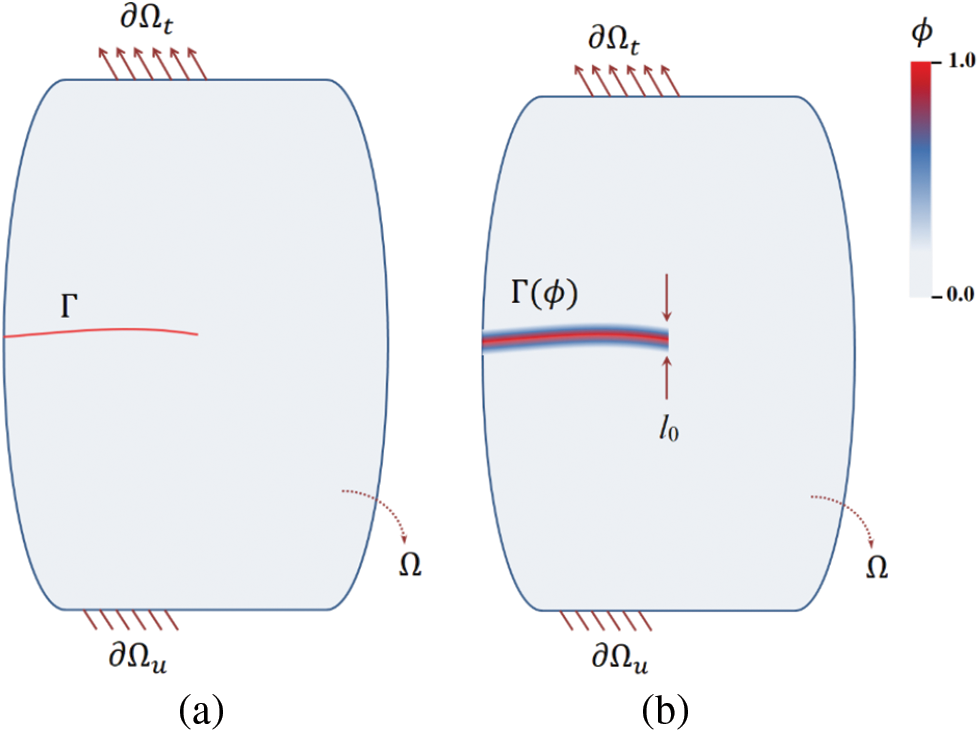
Figure 1: Schematic configuration of a solid continuum representing an internal crack as (a) sharp crack, and (b) diffuse crack

Within the phase-field model framework, the crack Γ(ϕ)⊂RNdim is smeared over the localization band X⊆Ω in the vicinity of the crack surface Γ(ϕ) and can be represented as a manifold of Ndim−1, with unit normal vector n^b. The crack emerges once a specific failure criterion is fulfilled. Here, we introduce the phase field ϕ(x) and its variation δϕ belonging to the Sobolev space (H1) as:

ϕ(x)∈𝒮ϕ:={ϕ∈H1(Ω)|ϕ(x)∈[0,1];ϕ˙(x)≥0∀x∈X}(3)

δϕ(x)∈𝒮δϕ:={δϕ∈H1(Ω)|δϕ(x)≥0∀x∈X;δϕ(x)=0∀x∈Γ}(4)

The energy dissipation (𝒟c) based on the principle of virtual work, guides the evolution of the crack in the continuum and can be expressed in terms of internal (𝒲int) and external work (𝒲ext) as [99]:

δ𝒟c=δ𝒲ext−δ𝒲int≥0(5)

The external work (𝒲ext) for prescribed body force vector (b¯) and boundary traction vector (t¯) on the reference configuration can be formulated as:

δ𝒲ext=∫Ωb¯⋅δudV+∫∂Ωt¯⋅δudA(6)

To couple the crack evolution with the deformation process in terms of the phase-field variable (ϕ) and the strain field ε(x)=∇symu(x), the associated internal work is expressed as a confluence of internal bulk energy (Ψb(ε,ϕ)=g(ϕ)⋅Ψ0(ε)) and dissipated energy (ΨΓ=Gc⋅γ(ϕ,∇ϕ)) due to the evolution of the crack,

δ𝒲int=∫ΩδΨb(ε,ϕ)dV+∫ΩδΨΓ(ϕ)dV(7)

The crack topology is defined in a regularized context in the localization band (X) as a crack density functional (γ) as follows [32]:

γ(ϕ,∇ϕ)=1c0[1l0α(ϕ)+l0|∇ϕ|2](8)

∀c0=4∫01α(z)dz=2(9)

The length scale parameter (l0) governs the width of the diffuse zone with c0>0 as a scaling factor and Gc as fracture energy. The crack geometric function α(ϕ)=ϕ2∀α∈[0,1] as per the standard AT-2 model is considered [28,100]. The energy degradation function, g(ϕ)=(1−ϕ)2+Kstab∀g(ϕ)∈[0,1], chosen as a quadratic polynomial function, describes the loss of strain energy density in the cracking solid. The stability parameter, considered as a small positive value (≈10−7−10−11) ensures residual stiffness once the material is fully damaged (ϕ=1). The energy degradation function satisfies the following properties:

g′(ϕ)<0,g(0)=1,g(1)=0 and g′(1)=0(10)

2.1 Constitutive Relations

The local strain energy density (Ψ0) can be accounted for as:

Ψ0(ε)=12ε:D0:ε=12σ¯:C0:σ¯(11)

The effective stress tensor (σ¯) for an isotropic elastic body is defined in terms of elastic stiffness (D0) and compliance (C0), respectively, as:

σ¯=D0:ε;ε=C0:σ¯;D0=C0−1(12)

D0=λ(I2⊗I2)+2μI4(13)

where Ij is jth order Identity tensor with λ & μ as Lame’s constants. The isotropic models consider that the strain energy density is degraded equally in the presence of compressive and tensile fields. To dissociate from this unphysical behaviour, anisotropy is considered as follows:

•   Volumetric-deviatoric split [30]

Ψ0(ε)⟶{Ψ0(ε)+=12K0⟨tr(ε)⟩2+μ(εdev:εdev)+Ψ0(ε)−=12K0⟨−tr(ε)⟩2(14)

•   Anisotropic split [41]

Ψ0(ε)±=λ2⟨tr(εi)⟩±2+μ⟨tr2(εi)⟩±(15)

ε=∑a=13εi[na⊗na](16)

with the Macaulay operator defined as ⟨V⟩±=V±|V|2 and K0=λ+2μ/3 as the bulk modulus. The constitutive relations can be expressed as:

σ=g(ϕ)⋅σ¯=∂Ψ(ε,ϕ)∂ε(17)

σ=∂∂ε[g(ϕ)Ψ0++Ψ0−]=g(ϕ)σ++σ−(18)

To ensure the irreversibility of damage, a history parameter is considered as the maximum positive reference energy subjected to Karush-Kuhn-Tucker (KKT) conditions [81] for loading and unloading as follows:

ℋ∗={Ψ0+(ε)Ψ0+>ℋnℋnotherwise(19)

2.2 Governing Equations

The variational of internal bulk energy (δΨb) and dissipation energy functional (δΨΓ) can be expressed as:

δΨb(ε,ϕ)=∫Ω[∂Ψb∂ε:∇symδu+∂Ψb∂ϕ:δϕ]dV=∫Ω[σ:∇symδu+∂Ψb∂ϕ:δϕ]dV(20)

⇒δΨb(ε,ϕ)=∫Ω[σ:∇symδu+g′(ϕ)ℋ∗δϕ]dV(21)

δΨΓ(ϕ)=Gcδγ(ϕ,∇ϕ)=∫ΩGcc0[1l0α′(ϕ)δϕ+2l0|∇ϕ|δ∇ϕ]dV(22)

The variational formulation of internal work can then be defined as:

δ𝒲int=∫Ω[σ:∇symδu+g′(ϕ).ℋ∗δϕ+Gcc0[α′(ϕ)l0δϕ+2l0|∇ϕ|δ∇ϕ]dV(23)

In accordance with the principle of virtual work and using the divergence theorem, the optimization condition δ𝒟c=δ𝒲ext−δ𝒲int≥0 yields,

∫Ωb¯⋅δu dV+∫∂Ωt¯⋅δu dA−∫Ω[σ⏞F:∇δu⏞∇G+g′(ϕ)⋅ℋ∗δϕ]dV+∫ΩGcc0[α′(ϕ)l0δϕ+2l0∇ϕ⏞F∇δϕ⏞∇G]dV=0(24)

Using the Divergence theorem, F⋅∇G=∇(FG)−∇F⋅G for manipulating the highlighted terms, the following set of governing equations is obtained:

∫Ω[∇⋅σ+b¯]δu dV+∫∂Ωt[t¯−σ⋅n]δu dA=0(25)

∫Ω{g′(ϕ)⋅ℋ∗+Gc[ϕl0−l0(Δϕ)]}δϕdV+∫∂ΩGcl0[∇ϕ.n^b]δϕdA=0(26)

here, n^b is the outward unit normal vector on the boundary ∂X, with Δ(.) representing the Laplacian operator.

2.3 Implementation of PFM with FEM

The nodal displacement field (u) and phase field (ϕ) in the computational domain are approximated via the matrix [Niu] and [Niϕ] in terms of the nodal displacements (ui) and phase-field (ϕi) degrees of freedom, respectively, as:

u=∑i=1mNiuui and ϕ=∑i=1mNiϕϕi(27)

where the element shape function matrix for the corresponding node i is defined as:

Niu=[Ni00Ni] and Niϕ=Ni(28)

The respective displacement-strain relation and damage gradient can then be defined as:

ε=∑i=1mBiuui&∇ϕ=∑i=1mBiϕϕi(29)

for Biu=[Ni,x00Ni,yNi,yNi,x]& Biϕ=[Ni,xNi,y](30)

The set of governing equations (Eqs. (25) and (26)) is solved in an iterative-incremental manner using the standard Newton-Raphson procedure. Since the energy functional (Eq. (5)) is non-convex for the set of unknowns (u,ϕ), it is reported that the standard monolithic approach delivers poor performance [37], the alternating minimisation strategy is employed [29] for solving the following system of equations:

[Ksϕ00Ksu]{ϕs+1us+1}={RsϕRsu}(31)

The corresponding residual vector and tangent matrix are expressed as follows:

Kϕ=∫Ω{[Gcl0+2ℋ∗](Nϕ)TNϕ+Gcl0(Bϕ)TBϕ}dV(32)

Ku=∫Ω{g(ϕ)(Bϕ)TD0Bϕ}dV(33)

Rϕ=−∫Ω{[g′(ϕ)ℋ∗+Gcl0ϕ](Nϕ)T+Gcl0(Bϕ)T∇ϕ}dV(34)

Ru=∫Ωg(ϕ)(Bu)Tσ¯dV−∫Ω(Nu)Tb¯dV−∫∂Ωt(Nu)Tt¯dA(35)

3  Refinement Strategy and Implementation Procedure in Abaqus

In the current finite element study, we have utilized the UEL and UMAT subroutines for numerical evaluation and post-processing [72]. In the adopted layered approach, 3-node and 4-node user elements are defined in the input file. The UMAT subroutine serves the dual purpose of post-processing and feedback for the MISESERI error indicator, which is a prerequisite for establishing the remeshing rule in Abaqus.

3.1 Error Indicators

The Abaqus module library offers the utility of various posteriori error indicators (e.g., MISESERI, ENDENERI, etc.) that can be used as output variables for numerical analysis. These error indicators develop the groundwork for adaptive remeshing in Abaqus, which can be prompted by a remeshing rule. The posteriori error indicators provide information about the region where discretization error potentially exists. These error indicators feature units identical to the base solution variable and can be requested as field output variables for individual elements. In the proposed refinement strategy, we have utilized the MISESERI error indicator variable as the basis of the remeshing. The MISESERI error indicator provides a discretization error estimate for the stress profile in the discretized specimen for the specified boundary conditions. The computations of this error indicator are based on the superconvergent patch recovery (SPR) technique, as reported in the literature [101 ]. A difference exists in the order of assumed trial functions for displacement and stress approximations. The stress values at the integration points are computed by employing a higher-order trial function whose order is the same as that of the displacement trial function. The energy norm distance between the values obtained by the smoothed estimation of the stress field and the non-smoothed estimation of the stress field serves as the value of the error estimate in the FEM solution. A detailed discussion on error estimation can be found in the literature [101–103].

3.2 Phase Field Implementation Using UEL and UMAT Subroutines

In Abaqus, the phase field implementation is accomplished by combining a UEL subroutine for integration point calculations and a UMAT subroutine for post-processing [72]. As a prerequisite, the UEL subroutine requires a ‘*_UEL.inp’ file, which contains the essential inputs regarding the nodal repository, element connectivity for user-defined elements, and a set of elements ‘umatelem,’ which serves as a dummy layer for post-processing via the UMAT subroutine. The initial input file ‘*.inp’ is generated by Abaqus itself for any analysis; however, for the phase field implementation, it is essential to define the user-defined elements, material, and fracture parameters and generate an element set for post-processing. All these essential data tweaks to the initial ‘*.inp’ file can be saved as ‘*_UEL.inp’ file, which can be used with the UEL subroutine for phase field implementation. The UEL subroutine requires the user to calculate the element’s tangent stiffness matrix (AMATRX) and force vector (RHS). The material and fracture parameters specified in the ‘*_UEL.inp’ file can be incorporated into the subroutine as an argument (*PROPS). The Abaqus solver interacts with the pre-defined array arguments of UEL to calculate and store results in the ‘*.odb’ file. The solution-dependent state variable array (STATEV) in the UMAT subroutine is utilized to post-process the results. The detailed implementation of this approach is reported in the literature [71,72].

3.3 Mesh Refinement Procedure for the Phase-Field Model

The proposed mesh refinement strategy for the phase field model is implemented entirely through Python scripting. The Python scripting utility’s goal is to automate this entire implementation process in a single pass, which is disassembled block-by-block, as illustrated in Fig. 2. The script contains appropriate functions/procedures for executing block-by-block operations simultaneously.

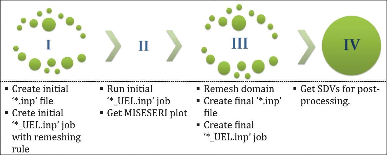
Figure 2: Block-wise overview of the mesh refinement procedure

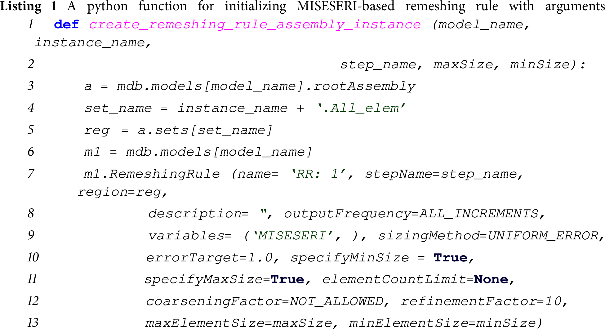
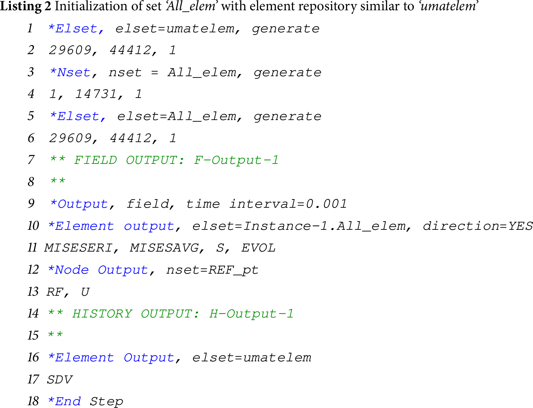
The process flowchart or the detailed operational plan depicting the algorithm for mesh refinement is shown in Fig. 3. The model geometry, user material data (with 16 dependent variables), section assignment, load step, boundary condition, amplitudes, etc., are defined initially through user-defined functions in the script. The discretization of the specimen geometry, the element type(s), and coarse mesh size is controlled via the script. The mesh refinement consists of two simultaneous steps: first reporting the error indicator as field output variables (from step I to step II in Fig. 2) and then remeshing the designated regions so the error estimate is within the tolerance limit. The tolerance limit is specified as errorTarget (refer to Listing 1) in the Remeshing Rule object for the whole domain. This tolerance limit for the numerical examples considered in the current work is kept in the range of 1%–5%, subjective to the type of problem. Two identical sets containing the element ids are defined in the input file—’umatelem’ and ‘All_elem’ (using *elset keyword in input file). The remeshing rule object is specified on the part set ‘All_elem’ as shown in Listing 1. It should be noted that defining this part set ‘All_elem’ is crucial for establishing the remeshing rule in Abaqus. The set ‘All_elem’ is the facsimile set with the same element connectivity as the ‘umatelem’ set (Listing 2). This guarantees that the field output variable values at the integration points in the elements of ‘umatelem’ set are also mapped to corresponding elements in this facsimile set within the solver’s data structure, therefore allowing the refinement to be triggered by the Remeshing Rule. The mesh parameters for executing mesh refinement can be specified as arguments to the RemeshingRule object (Listing 1) as ‘minElementSize’ and ‘maxElementSize’, both being subjective to the length scale parameter considered for the problem (h/l0).

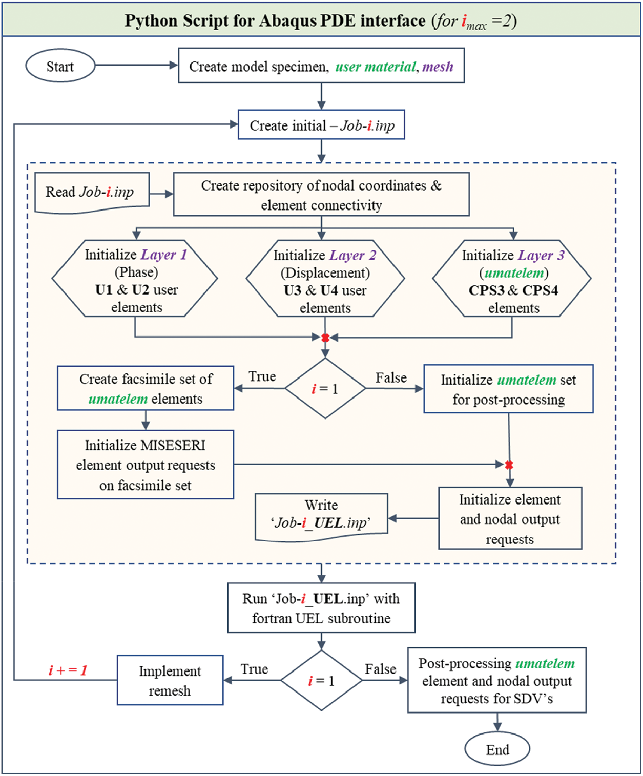
Figure 3: Flowchart for the Python based script for proposed mesh refinement implementation for phase-field model

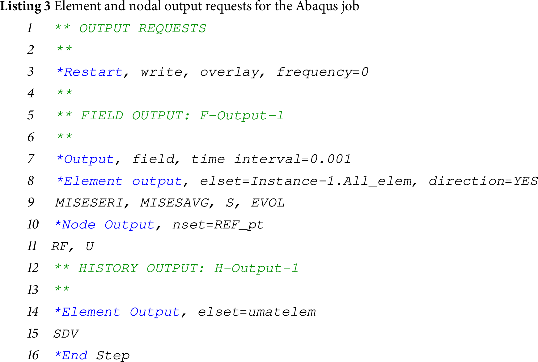
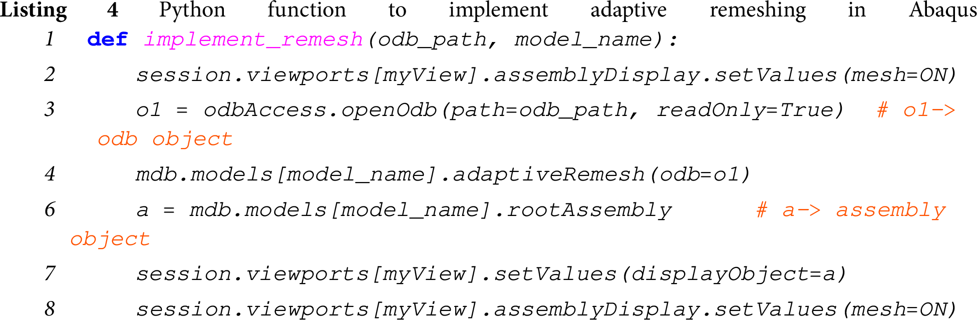
The first step of this automated process begins with defining the specimen’s geometry and initial coarse discretization which is stored in the input file—‘Job-1.inp’. The Python script extracts the element connectivity and nodal data from ‘Job-1.inp’. It then generates a modified input file—‘Job-1_UEL.inp’, which defines the layered system comprising user elements U1 & U2 (phase-field approximation), U3 & U4 (displacement approximation) and another layer for post-processing results, as documented in the literature [72]. The material and fracture properties are passed to the subroutine via ‘Job-1_UEL.inp’ as user element properties in the input file (using *UEL property keyword). Now, ‘Job-1_UEL.inp’ is submitted for analysis with the user subroutine to obtain the requested MISESERI values for the facsimile set ‘All_elem’, for each element (refer to Listing 3). The MISESERI values indicate regions that require local refinement, and then adaptive remeshing is implemented by calling a function ‘implement_remesh’ in the Python script that requires ‘*.odb’ file path and ‘model_name’ as arguments (refer to Listing 4). Abaqus utilizes its inherent refinement routines and the new refined mesh is registered. A new input file—‘Job-2.inp’ is again generated with the refined mesh data. Now, as we have obtained a refined mesh, a new input file ‘Job-2_UEL.inp’ is created and submitted along with the Fortran subroutine for numerical simulations. The readers are referred to the literature [72] for further insights into the method of running the phase-field simulations using UEL-UMAT subroutines. Solution-dependent variables (SDVs) are used to post-process the results.

4  Numerical Results and Discussion

In this section, the validity and robustness of the proposed mesh refinement strategy for PFM are validated through some of the benchmark fracture problems reported in the literature. All the numerical simulations are also performed for the standard PFM without the proposed remeshing strategy for comparative purposes. The results from the proposed strategy are compared with the standard PFM and the results from the available literature. The computational efficiency of the proposed PFM strategy is shown in a pie chart for all the problems considered. In all the problems, the model is discretized using triangular and quadrilateral elements in a non-uniform pattern. First, the standard problem of a single-edge notch plate under mode I and mode II loading conditions is considered for simulations. Further, a rectangular notched plate with a hole under the uniaxial tensile load is considered for simulation. Thereafter, the L-shaped panel test is conducted to assess the capacity of the proposed approach to capture the crack nucleation, growth, and failure in mixed-mode loading conditions. Finally, the tensile failure of multi-hole specimens in the absence of an initial crack is analyzed for two different geometries: a square panel with five and seven holes, respectively. The numerical tests are performed on an HP Desktop with an Intel(R) i7-7700 @ 2.80 GHz processor and 32 GB RAM.

4.1 Finite-Size Edge Crack Plate under Mode-I Loading

In the first example, a square plate with an edge crack of length 0.5 mm is considered for the simulations. The geometry and boundary conditions of the specimen are shown in Fig. 4a. The material properties of the specimen are taken from the literature [41] and are given as Young’s modulus, E = 210 GPa, and Poisson’s ratio, ν = 0.3. The length scale parameter, l0 = 0.0075 mm, and fracture energy, Gc = 2.7 × 10−3 KN/mm, are taken as fracture parameters.

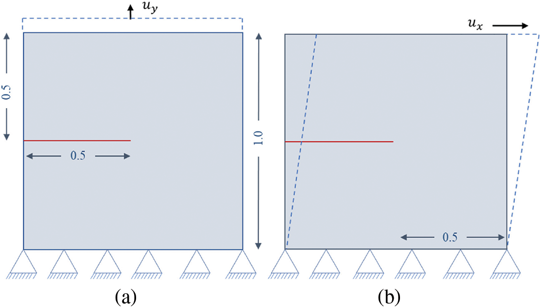
Figure 4: Single edge crack specimen geometry, dimensions and boundary conditions for (a) Mode-I loading (b) Mode-II loading

Firstly, the problem is simulated using standard PFM, where the model is discretized with 26,282 linear quadrilateral and linear triangular elements with a global mesh size of 0.02 mm. Further, the mesh is refined with mesh size h = 0.003 mm in the zone where the crack is expected to propagate (refer to Fig. 5). It is done by enforcing a suitable ratio of mesh size and length scale (h/l0 << 1) in the region. To simulate this problem, the anisotropic strain energy decomposition of Miehe et al. [32] with staggered implementation [72] in Abaqus is considered. The loading is applied via a displacement control strategy to determine the load variation to displacement. The displacement is applied in two steps. In the first step, the displacement u = 0.005 mm is specified for 2000 increments at increment size Δu1 = 10−4. In the second step, the displacement is ramped to u = 0.01 mm at Δu2 = 10−5 for the remaining increments. It is achieved by defining the tabular amplitudes for each Abaqus step separately. The predicted crack path for standard PFM is illustrated by plotting the contours of the phase field variable (ϕ), as shown in Fig. 5a, for different displacement points.

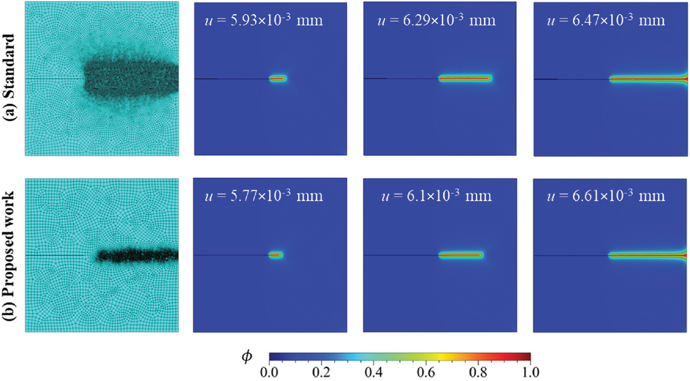
Figure 5: Discretized specimen and phase-field contours for (a) Standard and (b) Proposed PFM implementation for Mode-I loading condition at l0 = 0.0075 mm

Further, the proposed strategy for PFM is implemented in Abaqus using a Python script. The material and fracture parameters considered are similar to the standard PFM simulation.

The specimen is initially discretized with a global mesh size of 0.02 mm without local mesh refinement. A remeshing rule that governs the remesh region and global and local mesh size is established based on the MISESERI error indicator in the Abaqus utility for the whole specimen using Python scripting. To identify the MISESERI values, a displacement control scheme is applied with increment size Δu1 = 10−3 for 500 increments, followed by increment size Δu2 = 5 × 10−4 for the subsequent 1000 increments. Based on the MISESERI plot, the region shown in Fig. 6a has been designated as the one requiring mesh refinement. The adaptive remesh is then incorporated with a global mesh size of 0.02 mm and locally refined mesh size h = 0.001 mm, comprising 13,941 linear quadratic and triangular elements (refer to Fig. 5), which is quite less than the standard PFM. The phase field results for the proposed PFM are reported in Fig. 5b, which are similar to the standard PFM results. Further, the load-displacement responses for both methods, i.e., standard PFM and with the proposed PFM strategy, are compared in Fig. 7a, which agrees with the literature [32,41].

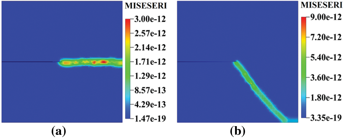
Figure 6: Error indicator plots for (a) Mode-I and (b) Mode-II loading

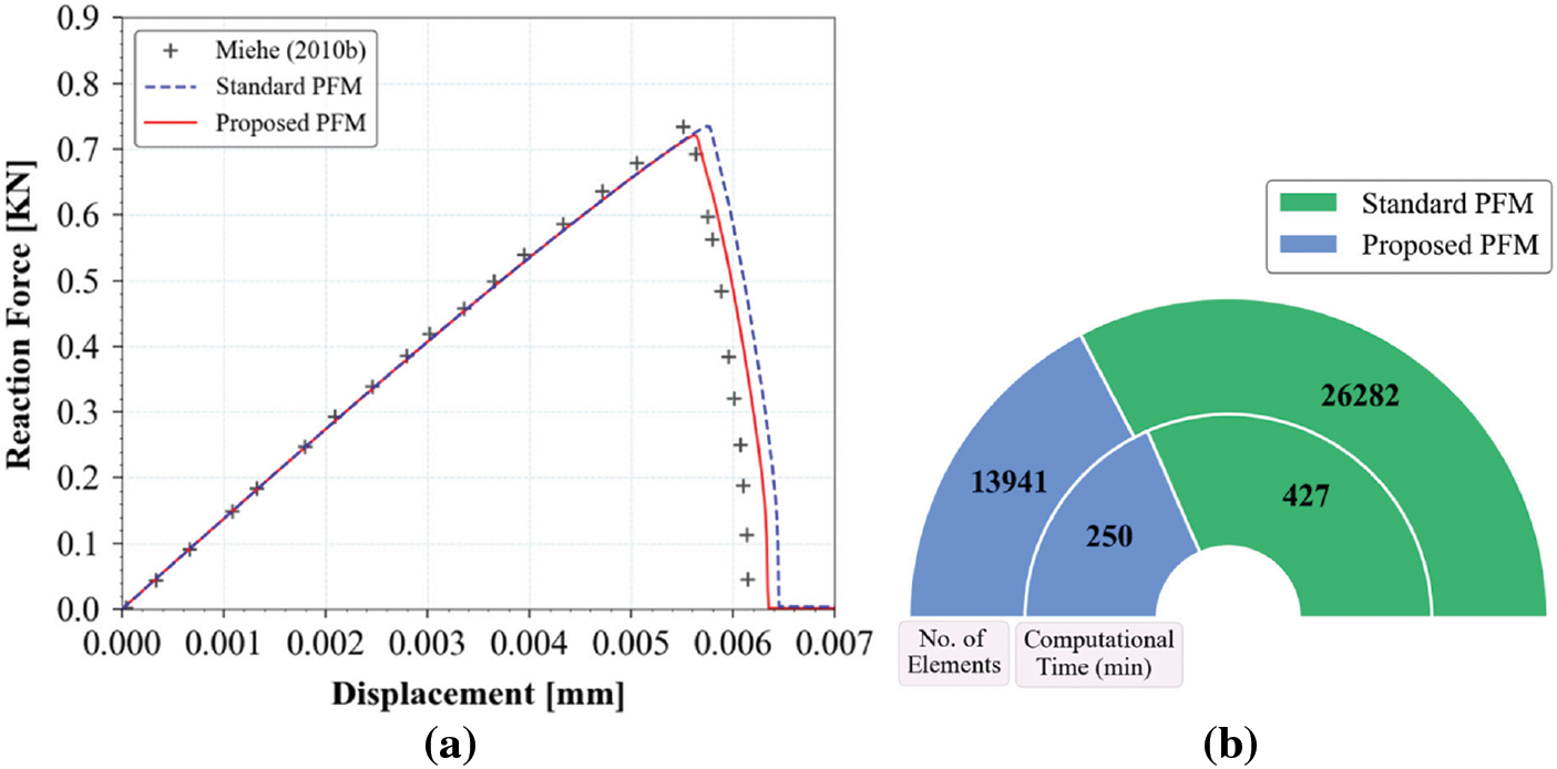
Figure 7: (a) Load-displacement response for single edge crack specimen under mode I loading, (b) Comparison of number of elements and computational time between standard PFM & proposed PFM

A comparison of computational efficiency for standard PFM and proposed PFM is shown in Fig. 7b. Compared to standard PFM, the global stiffness matrix size for the proposed PFM is about half, allowing for less memory requirement. The CPU time required to solve the problem in standard PFM is 427 min, whereas 250 min for the proposed PFM, indicating that the proposed PFM is more computationally efficient than the standard PFM. In the following subsections, the sensitivity of the proposed algorithmic framework to key parameters influencing the refined mesh density is systematically examined. At first, the influential parameters that directly or indirectly affect the mesh density are identified, i.e., the length scale parameter (l0), initial coarse mesh size, and the arguments of the Remeshing Rule (errorTarget, refinementFactor, etc.). Then, each case study is designed such that a single parameter is varied while the rest are kept constant, enabling a clear assessment of the individual impact on the resulting mesh refinement and the corresponding fracture response of the system. The condition numbers for different discretization are estimated to assess the numerical solution accuracy. The condition number measures sensitivity to input variations for a system of nonlinear equations. The condition number (Kcn) for a system of equations in the form Ax=B can be evaluated as Kcn=‖A−1‖⋅‖A‖. For the phase-field fracture model, the resulting system of nonlinear equations involves a global stiffness matrix of high dimensionality. Therefore, the evaluation of Kcn for such a high-order matrix seems not only computationally expensive. However, to probe the evolution of ill-conditioning, we propose an alternative method for the estimation of Kcn for the system. The primary source of nonlinearity in the system arises from the non-zero damage degrees of freedom. A suitable displacement step is considered near the peak load point in the mechanical response of the system. At this stage, a notable damage localization (in the range ϕ∈[0,1]) is observed near the notch tip. Beyond this point, the structural response indicates a reduction in the system’s load-bearing capacity.

The elements whose centroid falls within the region defined by 0.01≤ϕ≤1 are selected for assembling a damaged local stiffness matrix (Klocalϕ) at the representative displacement step.

This region can be generalized to be within the range (r¯dist=2l0). In this manner, the estimated Kcn serves as a reasonable proxy for understanding the system’s conditioning in the context of damage evolution.

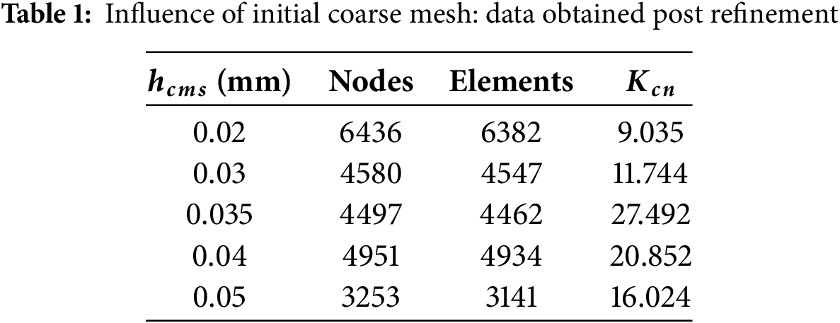
4.1.1 Influence of Initial Coarse Mesh Size (hcms)

In the first case study, we investigate the fracture response of the nonlinear system under the influence of varying initial coarse mesh sizes for Mode-I loading. The numerical simulations are performed considering a length scale parameter, l0 = 0.01 mm. The remeshing rule arguments are chosen as: errorTarget = 5 and refinementFactor = 10. The damage contour plots obtained with the considered parameters are shown along with the refined mesh in Fig. 8. It can be observed that with the proposed strategy, sufficiently good results are obtained with low initial coarse mesh sizes, but as the initial coarse mesh size is increased, erroneous error-indicator plots are reported. Consequently, refinement zones that are not feasible for accurate solutions are obtained. Thus, hcms= 0.03 mm can be selected for subsequent analysis, considering that further lowering the hcms might result in increased computational overhead. The statistics for this case study are reported in Table 1.

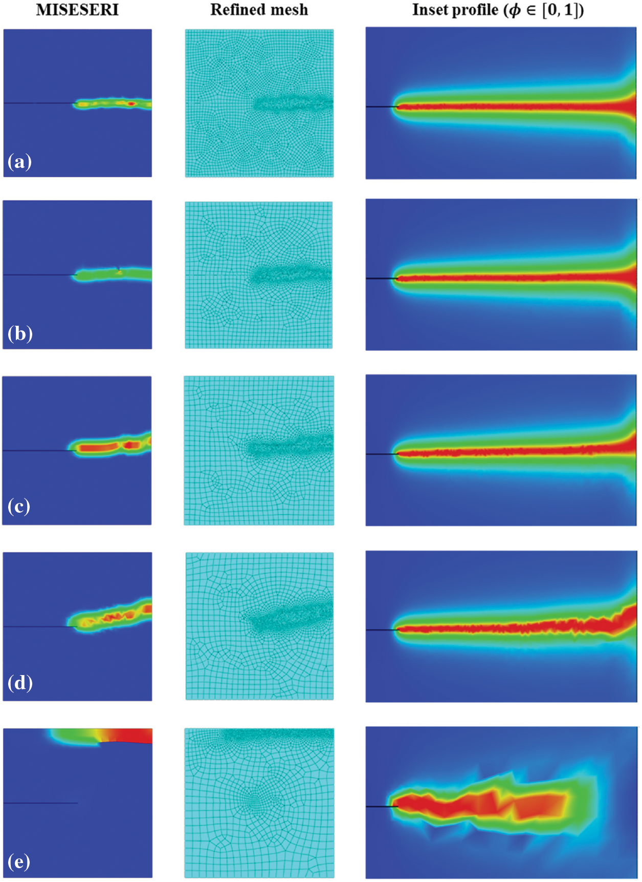
Figure 8: Influence of initial coarse mesh: Error indicator plots, refined mesh and inset phase-field contour plots for finite size edge crack plate under Mode-I loading for varying initial coarse mesh sizes (a) 0.02 mm (b) 0.03 mm (c) 0.035 mm (d) 0.04 mm (e) 0.05 mm

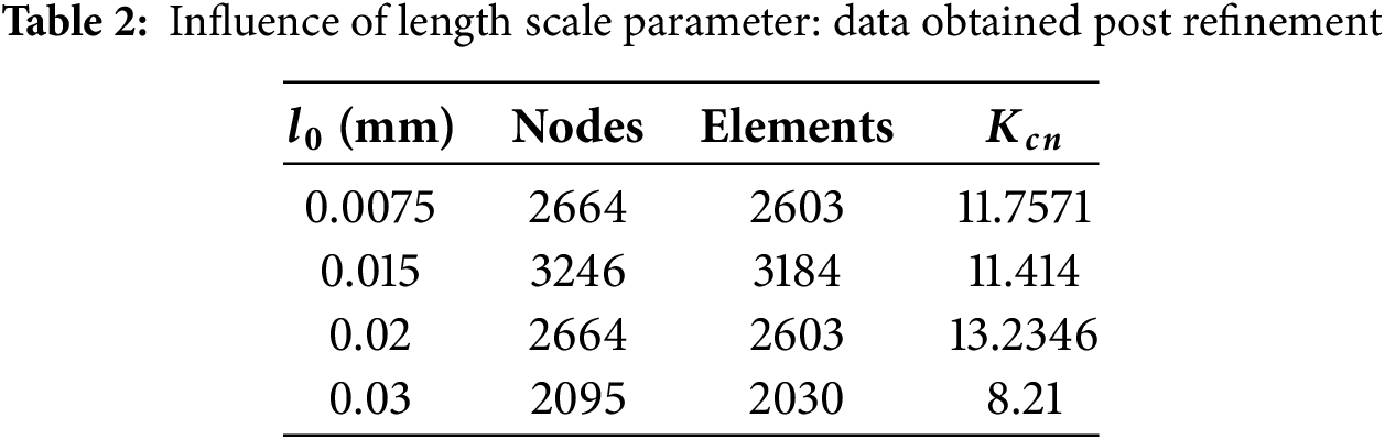
4.1.2 Influence of the Length Scale Parameter

Next, we consider varying the length scale parameter and investigating its influence on the overall refinement profiles. Based on the numerical solutions of the preceding subsection, hcms = 0.03 mm is considered the optimal mesh size. The rest of the key parameters (errorTarget and refinementFactor) are similar to those in the previous case study. The numerical tests are conducted for l0∈ {0.0075, 0.015, 0.02, 0.03} mm. The contour plots for phase-field, error indicator MISESERI and refined mesh are illustrated in Fig. 9. The contour plots indicate that while the numerically obtained crack paths are generally similar, the adaptive solutions corresponding to larger length scales (l0 = {0.02, 0.03}) exhibit reduced smoothness compared to those associated with smaller length scales. This behavior can be attributed to insufficient mesh refinement under the current values of adaptivity parameters for the Remeshing Rule object (errorTarget and refinementFactor), suggesting a practical need for further numerical investigations. As per the observations, a length scale value of 0.01 mm would be practical for further simulations of a finite-size edge crack plate under Mode-I loading. The statistics for this case study are reported in Table 2.

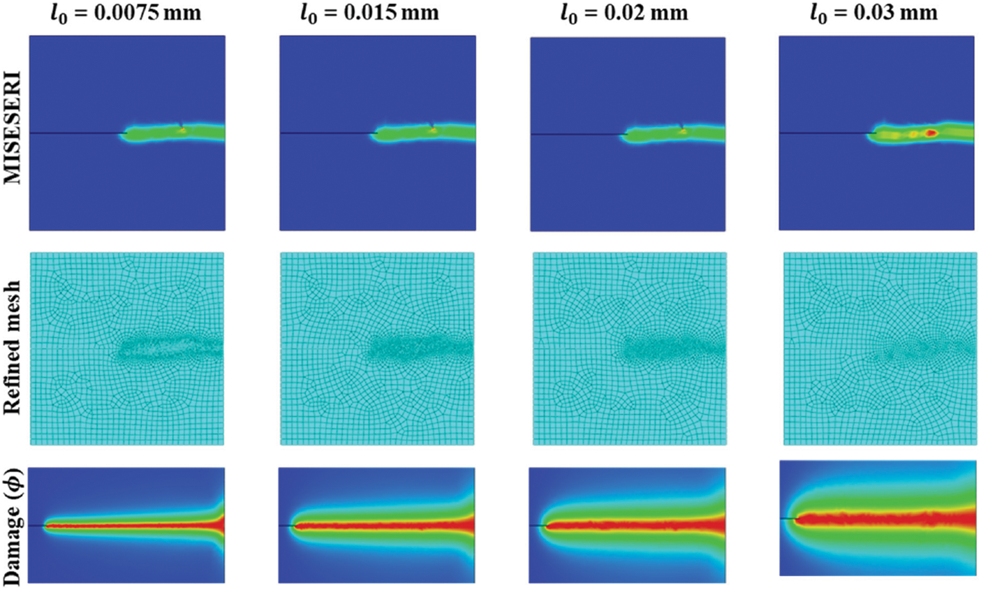
Figure 9: Influence of length scale parameter: Error indicator plots, refined mesh and inset phase-field contour plots for finite size edge crack plate under Mode-I loading for varying l0

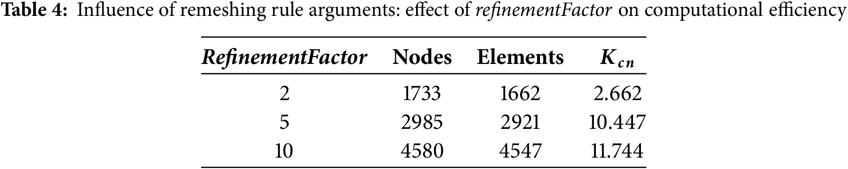
4.1.3 Influence of Remeshing Rule Arguments

In this subsection, we investigate the influence of two major arguments of the Remeshing Rule object, i.e., values of errorTarget and refinementFactor chosen for the numerical simulations using the proposed strategy. The numerical tests are first considered for l0 = 0.01 mm, hcms = 0.03 mm, refinementFactor = 10 with varying errorTarget values ∈ {2, 5, 10, 20}. In this case study, both l0 and hcms are kept constant. Consequently, as expected, the resulting MISESERI plots are nearly identical for all the cases. The extent and intensity of mesh refinement, however, are governed by the errorTarget parameter, as demonstrated by the refined mesh and damage contour plots (see Fig. 10). From the figure, it is evident that errorTarget implicitly controls the spatial extent of the refinement region. Accordingly, for a fixed l0, a higher value of errorTarget leads to a less dense refined zone, which in turn results in reduced solution accuracy in obtaining the crack paths. A summary of the post refinement statistics is presented in Table 3. While using a lower errorTarget in subsequent numerical simulations could enhance the solution accuracy, it might result in additional computational overheads. Therefore, the errorTarget value of 5 for numerical analysis is considered a practical choice for further numerical analysis, as it provides a favorable balance between accuracy and computational efficiency. Using this errorTarget value, we next vary the refinementFactor ∈ {2, 5, 10}. As the name implies, it controls the degree of refinement within the marked region. The corresponding contour plots and refined mesh profiles are presented in Fig. 11. Almost negligible mesh refinement is observed for lower values of refinementFactor. As indicated in Table 4, increasing refinementFactor from 5 →10 does not significantly affect the conditioning of the nonlinear solution system. Henceforth, refinementFactor = 10 is adopted for the rest of the simulations.

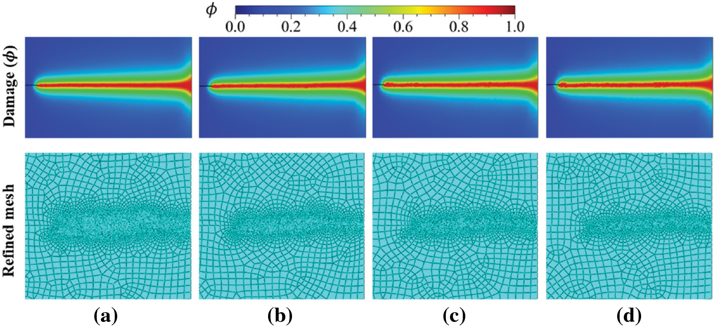
Figure 10: Influence of Remeshing Rule arguments: inset plots for phase-field and refined mesh for finite size edge crack plate under Mode-I loading for varying errorTarget values: (a) 2 (b) 5 (c) 10 (d) 20

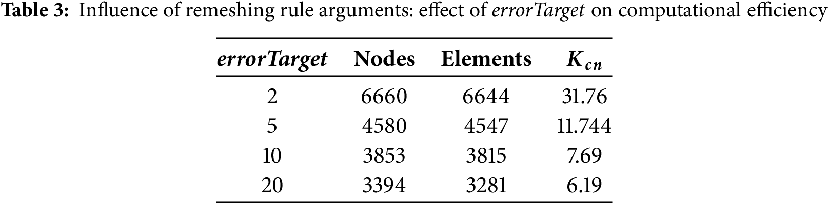
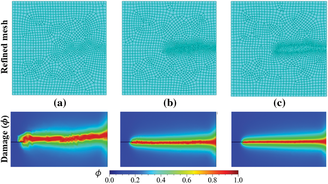
Figure 11: Influence of Remeshing Rule arguments: refined mesh and inset phase-field contours for finite size edge crack plate under Mode-I loading for varying refinementFactor values: (a) 2 (b) 5 (c) 10

4.2 Finite-Size Edge Crack Plate under Mode-II Loading

In this section, the problem considered in Section 4.1 is simulated under shear loading conditions, as shown in Fig. 4b. The bottom edge is kept fixed (ux = uy = 0), and horizontal displacement is applied at the top edge of the plate. It is a standard fracture problem in the literature to analyze the capacity of a method to dissociate diffuse crack topology based on tensile and compressive fields. Anisotropic split by Miehe et al. [41] is employed in this problem. The material properties, such as Young’s modulus (E), Poisson’s ratio (ν) are taken similar to the previous section. For the given problem, the fracture parameters, i.e., length scale, l0 = 0.015 mm and fracture energy, Gc = 2.7 × 10−3 KN/mm, are considered for implementation in both standard PFM and proposed mesh refinement PFM.

The crack is expected to grow towards the bottom edge, inclining to the right corner of the panel [32,72]. The deflected crack’s precise path cannot be determined; hence, a broad zone with a high mesh density must be established where crack propagation is anticipated. The finite element model of the specimen in Abaqus for standard PFM is discretized with 37,155 elements of a global mesh size of 0.04 mm with a refined mesh size of 0.003 mm, as shown in Fig. 12a. The displacement is applied in two simultaneous Abaqus steps with a median of 0.06 mm at increment size Δu1 = 10−5 for 2000 increments and Δu2 = 10−6 for the rest of the increments, respectively. The phase field contours for standard PFM are shown in Fig. 12a for multiple displacement values.

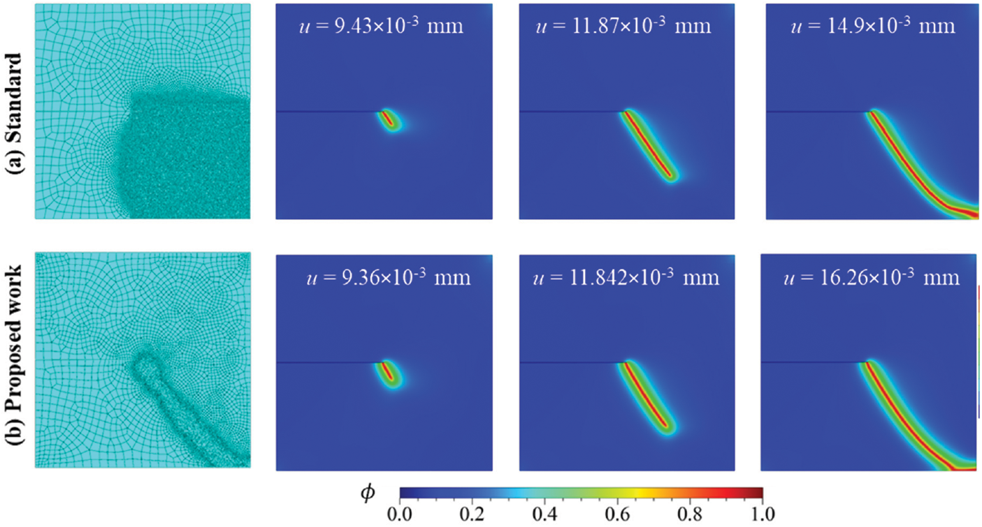
Figure 12: Discretized specimen and phase-field contours for (a) Standard and (b) Proposed PFM implementation for Mode-II loading condition at l0 = 0.015 mm

Further, the proposed PFM is applied to model the crack topology for the mode II loading scenario. The pre-adaptive ‘Job-1_UEL.inp’ is submitted for 2100 increments of size Δu1 = 5 × 10−4 and then at Δu2 = 10−5 for a further 5000 increments. The initial mesh with the global mesh size of 0.02 mm is analyzed for the MISESERI error indicator values. The MISESERI plot demarcating the crack propagation region is presented in Fig. 6b. The MISESERI plot demonstrates the effective tracking of the predicted crack direction. The error indicator-based adaptively refined mesh is shown in Fig. 12b with 19,963 elements. The functions implement the refinement scheme (refer to Listings 1 and 4) present in the Python script, and the final job, i.e., ‘Job-2_UEL.inp’ is submitted in conjunction with the Fortran subroutine according to the algorithm given in Fig. 3. The results of the proposed PFM are illustrated in Fig. 12 for different displacement points, which are quite similar to the standard PFM.

The load vs. displacement response for both standard PFM and proposed PFM is shown in Fig. 13a, which reasonably agrees with the literature [73]. Beyond the displacement u = 15 × 10−3 mm, the structural response of the proposed PFM exhibits a little more relaxation than the standard PFM, where the diffuse crack reaches the bottom edge of the specimen earlier. Fig. 13b compares the standard PFM and the proposed PFM, demonstrating that the proposed PFM implementation in Abaqus outperforms the standard PFM regarding the computational expense. The computing time for the proposed PFM is 471 min, almost half of that for the standard PFM in Abaqus.

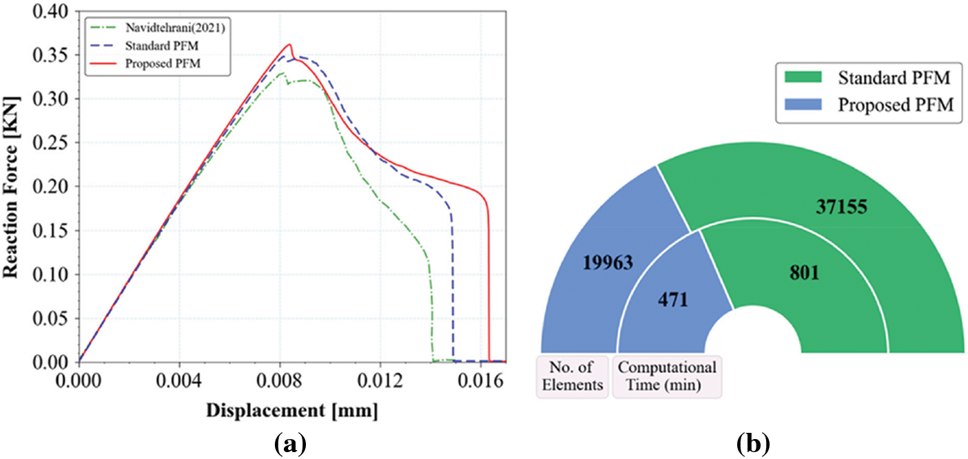
Figure 13: (a) Load-displacement response for single edge crack specimen under Mode-II loading, (b) Comparison of number of elements and computational time between standard PFM & proposed PFM

4.3 Rectangular Notched Plate with a Hole

This problem is considered to examine the ability of the proposed mesh refinement strategy for PFM to capture the influence of significant voids on the crack path. The presence of a hole in front of the notch in the specimen ensures the induction of a mixed-mode loading scenario. The notch width is taken as 0.4 mm. The experimental analysis of this problem was previously conducted by Ambati et al. [39], which reports the nucleation of two crack profiles, one from the notch and the other one from the edge of the hole. For imposing the boundary conditions, the lower hole is kept fixed while the incremental displacement is applied at the upper hole, as shown in Fig. 14. The experimentally observed crack path domain is illustrated in Fig. 15a. The material properties, such as Young’s modulus, E = 210 GPa, and Poisson’s ratio, ν = 0.3, are taken from the literature [62]. The length scale parameter, l0 = 0.285 mm, and fracture energy Gc = 2.28 × 10−3 KN/mm are taken as fracture parameters. The anisotropic formulation of Miehe et al. [32] is considered for both standard PFM and proposed PFM.

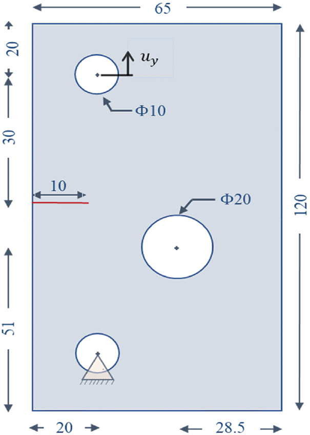
Figure 14: Geometry and boundary conditions of rectangular notched plate with hole

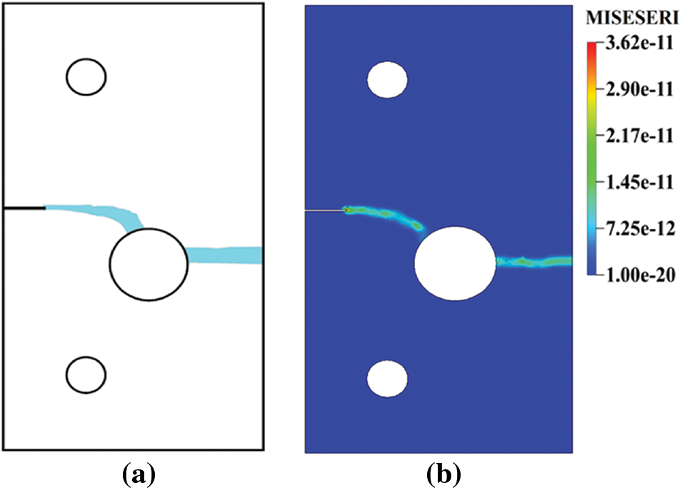
Figure 15: (a) Experimentally observed crack path [39] and (b) error indicator plot for a rectangular notched plate with a hole

For standard PFM implementation, the specimen is discretized with the global mesh size of 2 mm with a local refinement of h = 0.143 mm, constituting approximately 86,000 linear triangular and quadrilateral elements as shown in Fig. 16a. The displacement is applied in two Abaqus steps with increment sizes Δu1 = 5 × 10−4 and Δu2 = 2 × 10−4 for 2000 and 4000 increments, respectively, to ensure the structural response is well recorded. The standard PFM numerical crack path prediction is illustrated in Fig. 16a for the marked loading points s1–s4 (see Fig. 17a), and is found to be in good agreement with the experimental analysis results [39].

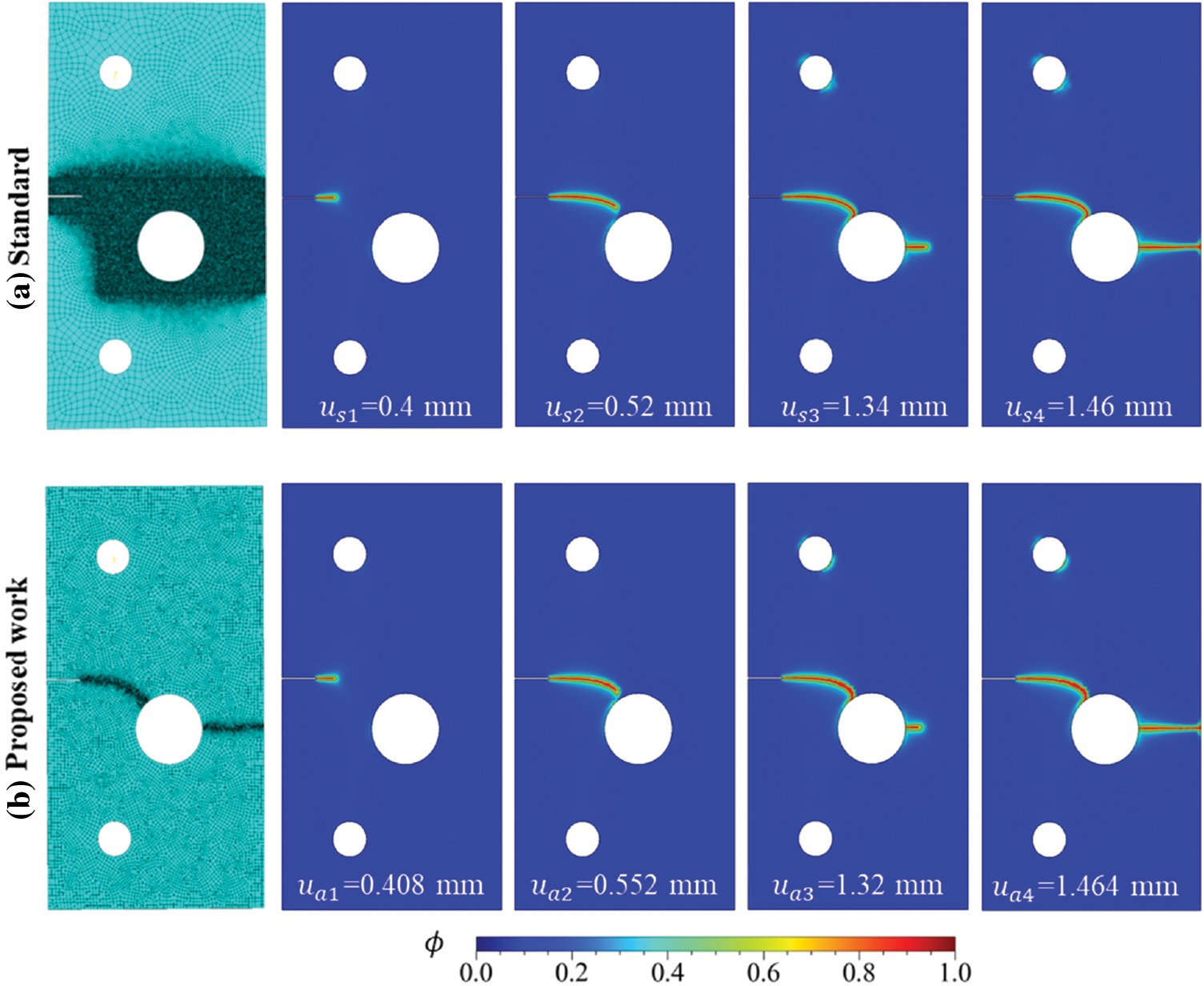
Figure 16: Discretized specimen and phase-field contours for (a) Standard and (b) Proposed PFM implementation for rectangular notched plate with hole at l0 = 0.285 mm

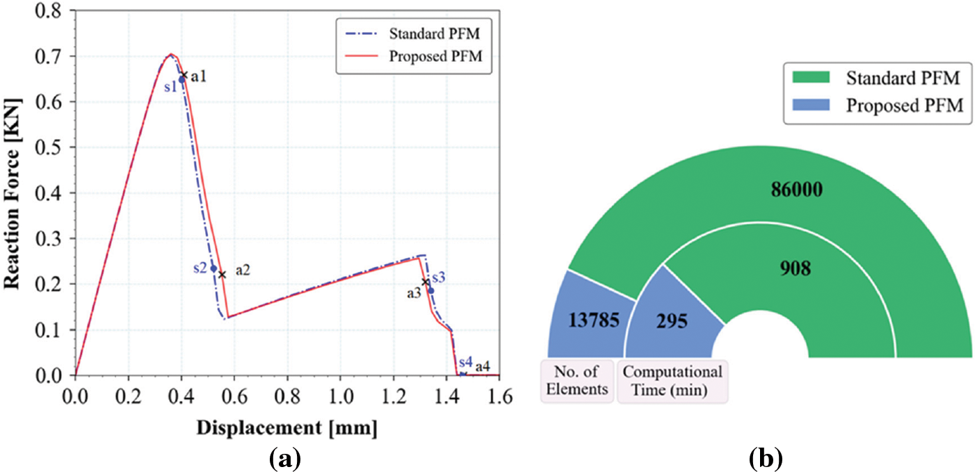
Figure 17: (a) Load-displacement response for rectangular notched plate with a hole, (b) Computational time and number of elements comparison between standard PFM and proposed PFM

Further, the proposed mesh refinement strategy in PFM is implemented by defining the initial global mesh size of 1.5 mm for the whole specimen. The MISESERI plot is obtained as shown in Fig. 15b. The Python script specifies two specific functions for initializing the remeshing rule (refer to Listing 1) and its implementation (refer to Listing 3). The remeshing rule refines the mesh in the marked regions with local mesh refinement size h = 0.143 mm. The post-adaptive discretized specimen, as depicted in Fig. 16b, is used to generate the new element and nodal repository (Job-2.inp file) through the Python script. Next, the ‘Job-2_UEL.inp’ is submitted along with the Fortran subroutine to obtain phase field results for the proposed PFM as shown in Fig. 16b, corresponding to the displacement points a1 to a4 in the structural response of the system.

The structural responses for standard PFM and proposed PFM are compared in Fig. 17a and are found to be in agreement. The diffuse crack that emerges from the notch develops to a state where the crack reaches the boundary of the hole in the specimen, following a curved path. As the displacement increases, the second crack emerges from the hole’s boundary. The observations from both approaches are in coherence with those reported in the literature [39]. A comparative analysis between standard PFM and proposed PFM is presented in Fig. 17b. The proposed PFM results are obtained in 295 min, while the standard PFM takes 908 min. Thus, a significant reduction in computational time is observed for the proposed PFM compared to the standard PFM. The order of AMATRX for standard PFM is almost six times that of the proposed PFM, which signifies that the latter provides considerable savings in memory requirements.

4.4 L-Panel Test

This section considers a mixed-mode failure problem of an L-shaped panel for the analysis. The geometry, dimensions, and loading conditions are shown in Fig. 18. The bottom edge is fixed, while the incremental displacement is applied at 30 mm from the right edge in the upward direction as shown in the figure. The experimental analysis of this problem has been reported in the literature [104], and the experimentally observed crack path is depicted in Fig. 19a. This fracture study is commonly considered a validation benchmark for the crack path obtained from the numerical results. The material properties are considered Young’s modulus, E = 25.84 GPa, and Poisson’s ratio, ν = 0.18. The length scale parameter, l0 = 3.125 mm, and fracture energy, Gc = 9.5 × 10−5 KN/mm, are taken as fracture parameters from the literature [105]. The thickness of the L-panel is taken as 100 mm.

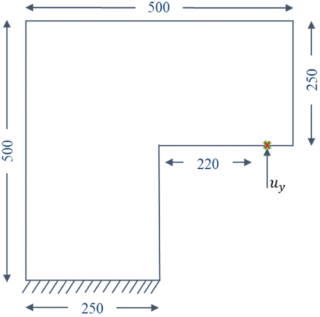
Figure 18: Geometry and boundary conditions for L-panel specimen

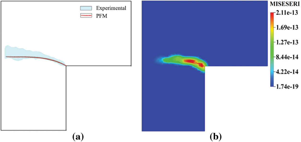
Figure 19: (a) Experimentally observed crack path [104] and (b) error indicator plot for L-panel test

First, an L-shaped panel is simulated using standard PFM by discretizing the geometry with a global mesh size of ≈17 mm. A local mesh refinement with element size 0.625 mm (h/l0 = 0.2) is adopted for the region depicted in Fig. 20a. The whole domain is discretized with a non-uniform mesh consisting of 55,625 linear triangular and quadrilateral elements. A net displacement of 1 mm is applied in two steps at increment sizes of Δu1 = 10−5 and Δu2 = 10−6 for 1000 and 2000 increments, respectively, to ensure the structural response is well recorded. The structural response for the standard PFM is shown in Fig. 21a. The numerically predicted diffused crack pattern for standard PFM is illustrated in Fig. 20 for different displacement points (s1 to s3).

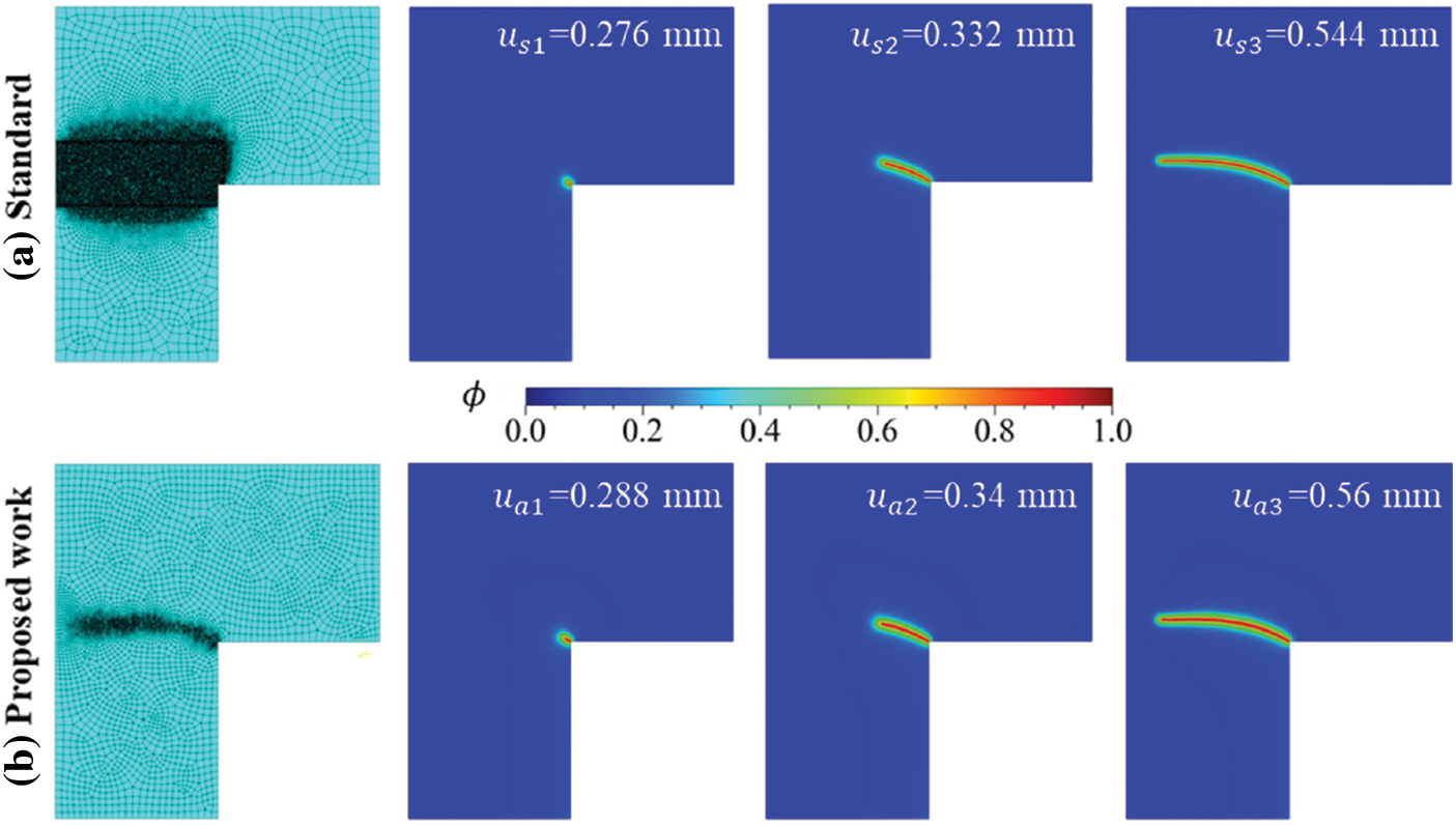
Figure 20: Discretized specimen and phase-field contours for (a) Standard and (b) Proposed PFM implementation for L-panel test at l0 = 3.125 mm

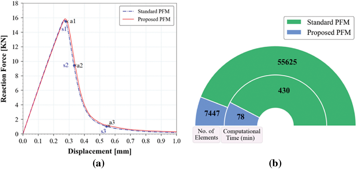
Figure 21: (a) Load-displacement response corresponding for L-shaped panel and (b) Computational time and number of elements comparison between standard PFM and proposed PFM for the L-shaped panel

Next, the L-shaped panel is simulated using the proposed strategy. The material and fracture parameters are kept the same as in standard PFM. Initially, the global mesh size was 12 mm for the whole model, with no local mesh refinement. The region that requires local mesh refinement is obtained with the help of MISESERI values. For the initial ‘Job-1_UEL’, a net displacement of 1 mm is applied in two steps with increment sizes of Δu1 = 10−3 and Δu2 = 10−4 for 1000 and 2000 increments, respectively, and the corresponding MISESERI plot is shown in Fig. 19b. The error-target value for the remeshing rule is kept at a numerical value of 3.5 on a ‘UNIFORM_ERROR’ basis for the current example. The global mesh size and local mesh size (h) are specified in the remeshing rule for the arguments ‘maxElementSize’ and ‘minElementSize’ (Listing 1) as 15 mm and 0.625 mm, respectively. The adaptively refined mesh for the L-shaped panel is depicted in Fig. 20b. The nodal coordinates and element connectivity repository are read from ‘Job-2.inp’ via the Python script, and the input file ‘Job-2_UEL.inp’ required for final phase field results is developed. The incremental displacement of Δu1 = 10−5 and Δu2 = 10−6 for 1000 and 2000 increments, respectively, is applied to ensure the accurate structural response for the proposed PFM. The phase field results for the proposed PFM are shown in Fig. 20b, corresponding to the points a1 to a3 marked in Fig. 21a. A good agreement between the standard PFM and proposed PFM regarding the crack path and structural response is observed, which signifies that the proposed refinement strategy for PFM can successfully track the crack evolution mechanism for the L-shaped panel test.

The comparison metrics for standard PFM and proposed PFM are presented in Fig. 21b. The computational time required for standard PFM is 352 min more than that of the proposed PFM. Also, the memory requirement for later is found to be almost one-seventh of that of standard PFM.

4.5 Tensile Failure of a Square Plate with Five Holes

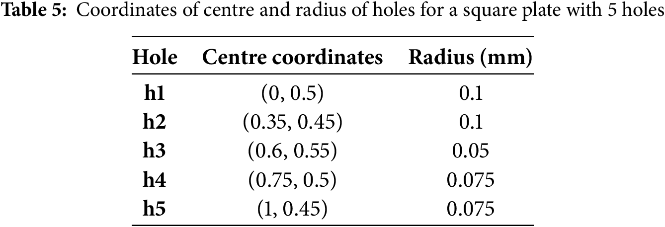
The tensile failure of a square plate with five holes without any initial crack is considered for the numerical analysis. The objective of studying this problem is to demonstrate the capacity of the proposed mesh refinement strategy to capture the crack nucleation and growth in the presence of multiple voids or defects in the absence of any pre-existing crack. Fig. 22a shows the geometry and the applied boundary conditions. The specimen consists of two semi-circular holes at the left and right edges and three circular holes of different radii within the specimen [106]. The holes’ geometric centres and radii are specified in Table 5. The volumetric-deviatoric energy split by Amor et al. [30] is implemented in the Fortran subroutine for this problem.

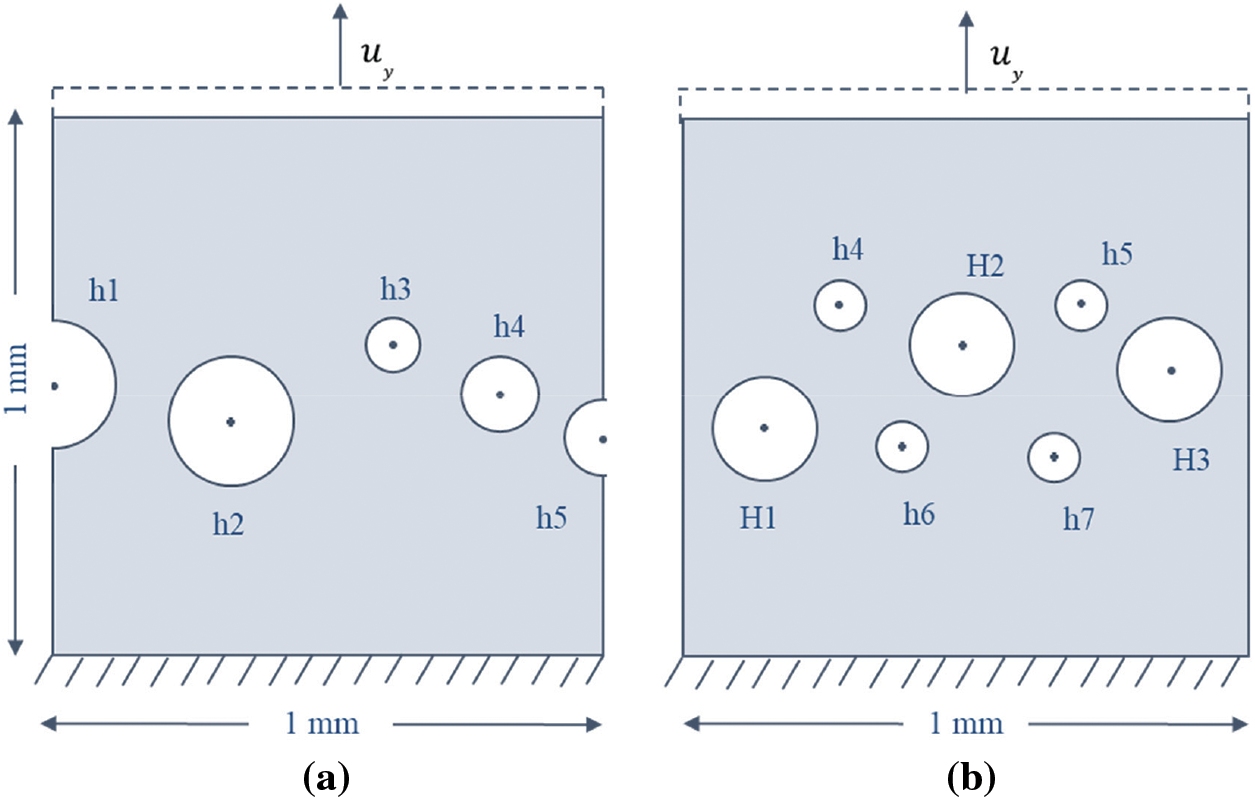
Figure 22: Geometry and boundary conditions for a square plate with (a) 5 holes and (b) 7 holes

The problem is first simulated using the standard PFM method. The discretized specimen consisting of 45,399 linear triangular and quadrilateral elements is shown in Fig. 23a. The total displacement uy = 0.01 mm is applied in two steps. In the first step, the increment size Δu1 = 10−4 for 2000 increments; for the second step, the increment size Δu2 = 5 × 10−5 for 5000 increments is specified. The crack nucleation initiates near the hole h5, with a similar but much subdued nucleation near h4. Further, the crack grows along h3 and h2 with a modest increase in displacement. The crack growth mechanism observed between h5 and h4 exhibits distinct characteristics from that observed for crack growth from h4 to h2. The crack growth trajectory for standard PFM corresponding to the points marked in Fig. 24a is depicted in Fig. 23a and agrees with the literature [106].

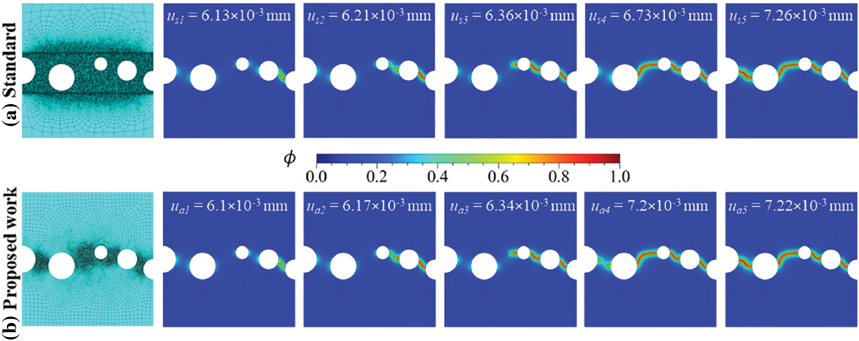
Figure 23: Discretized specimen and phase-field contours for (a) Standard PFM and (b) Proposed PFM implementation for square plate with 5 holes at l0 = 0.008 mm

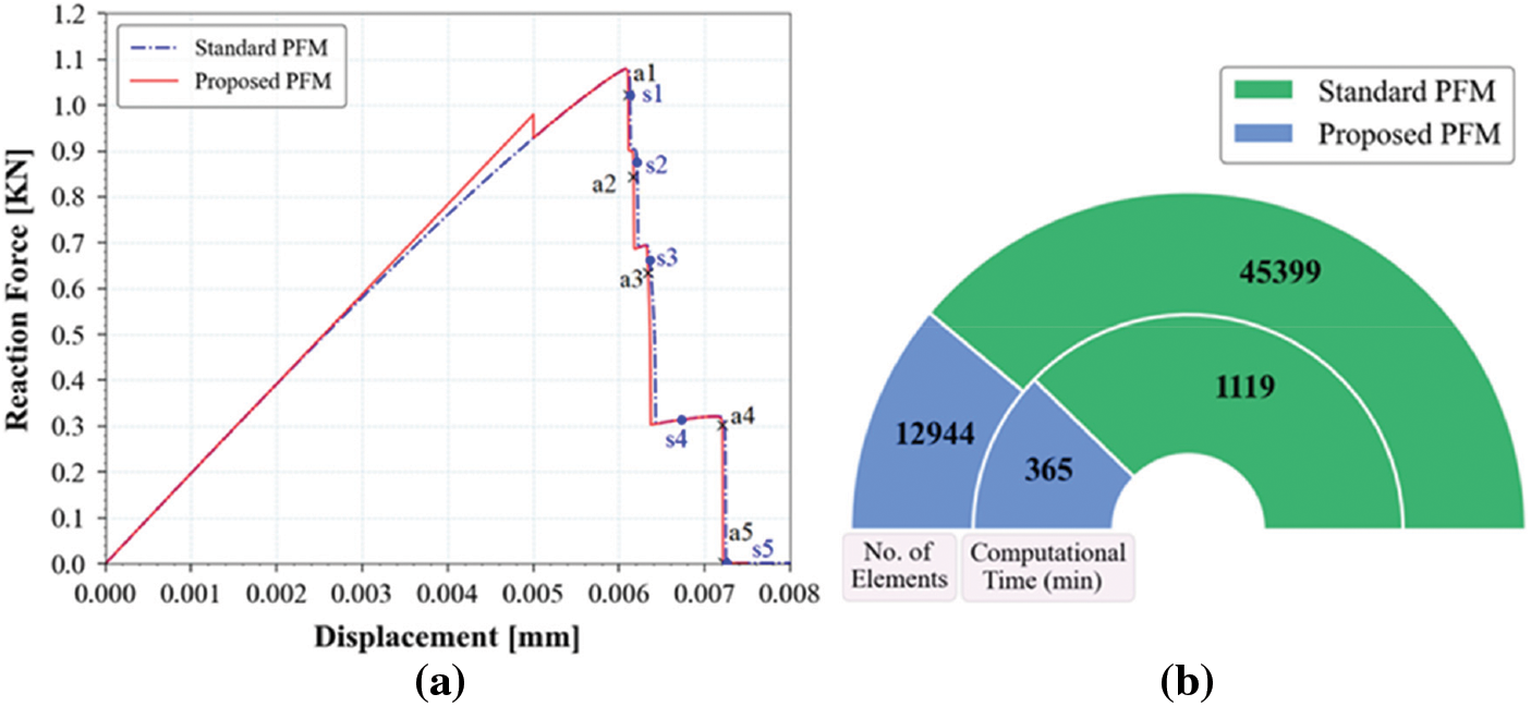
Figure 24: (a) Load-displacement response for square plate specimen with 5 holes, (b) Computational time and number of elements comparison between standard PFM and proposed PFM

Further, as discussed previously, the mesh refinement strategy implementation in PFM is executed via a two-job process. The specimen is first discretized coarsely with a global mesh size of 0.02 mm. The ‘Job-1_UEL.inp’ is submitted along with the Fortran subroutine to obtain the MISESERI values. The MISESERI plot is depicted in Fig. 25a. The MISESERI plot represents the region requiring local mesh refinement, which is implemented through the remeshing rule specified in Listing 4. The adaptive remeshing enables a local mesh refinement of size h = 0.001 mm and a global mesh of size of 0.3 mm, constituting 12,944 elements, as shown in Fig. 23b. The phase field results for the proposed PFM are shown in Fig. 23b, corresponding to the points marked in Fig. 24a. The crack growth pattern and mechanism for the proposed PFM are similar to those observed in standard PFM results and literature [106].

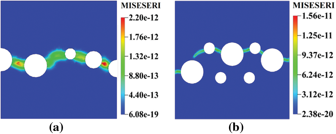
Figure 25: Error indicator plots for a square plate specimen with (a) 5 holes and (b) 7 holes

The load vs. displacement plot for standard PFM and proposed PFM is reported in Fig. 24a. The number of elements and computational time are presented in Fig. 24b. The computational time for standard PFM and proposed PFM is 1119 min and 365 min, respectively. Therefore, from the simulations, it can be concluded that the proposed PFM is computationally much more efficient for simulating such a problem.

4.6 Tensile Failure of a Square Plate with Seven Holes

In the last example, a square plate with seven holes, as shown in Fig. 22b, is considered for the numerical analysis. The material properties and fracture parameters are the same as in Section 4.5. The radius and coordinates of the centre of the holes are reported in Table 6. The standard PFM simulations are carried out for specimens discretized with 81,090 linear triangular and quadrilateral elements with a global size of 0.03 mm. The local mesh refinement, h = 0.002, is made in the region where the crack is expected to grow, as shown in Fig. 26a. The net displacement in the increment size Δu1 = 10−4 for 3500 increments and Δu2 = 2 × 10−6 for the further 10,000 increments is applied. The phase field contours for standard PFM are shown in Fig. 26a and are found to be in agreement with those reported in the literature [106].

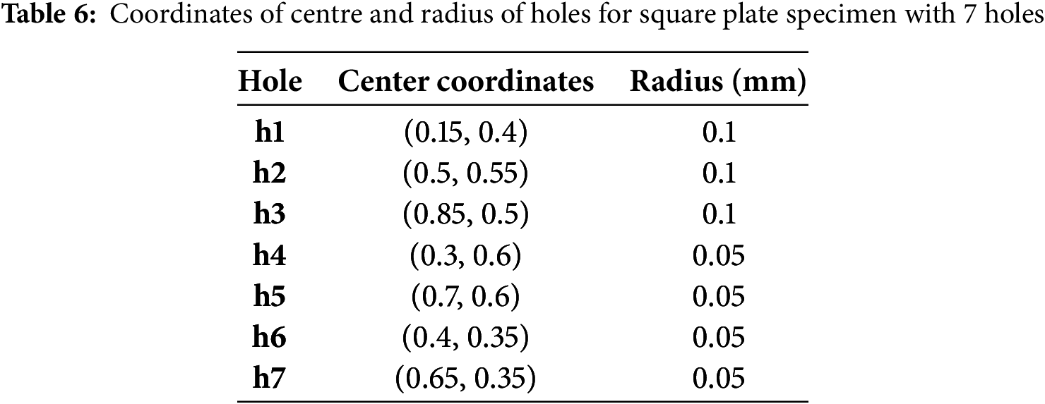
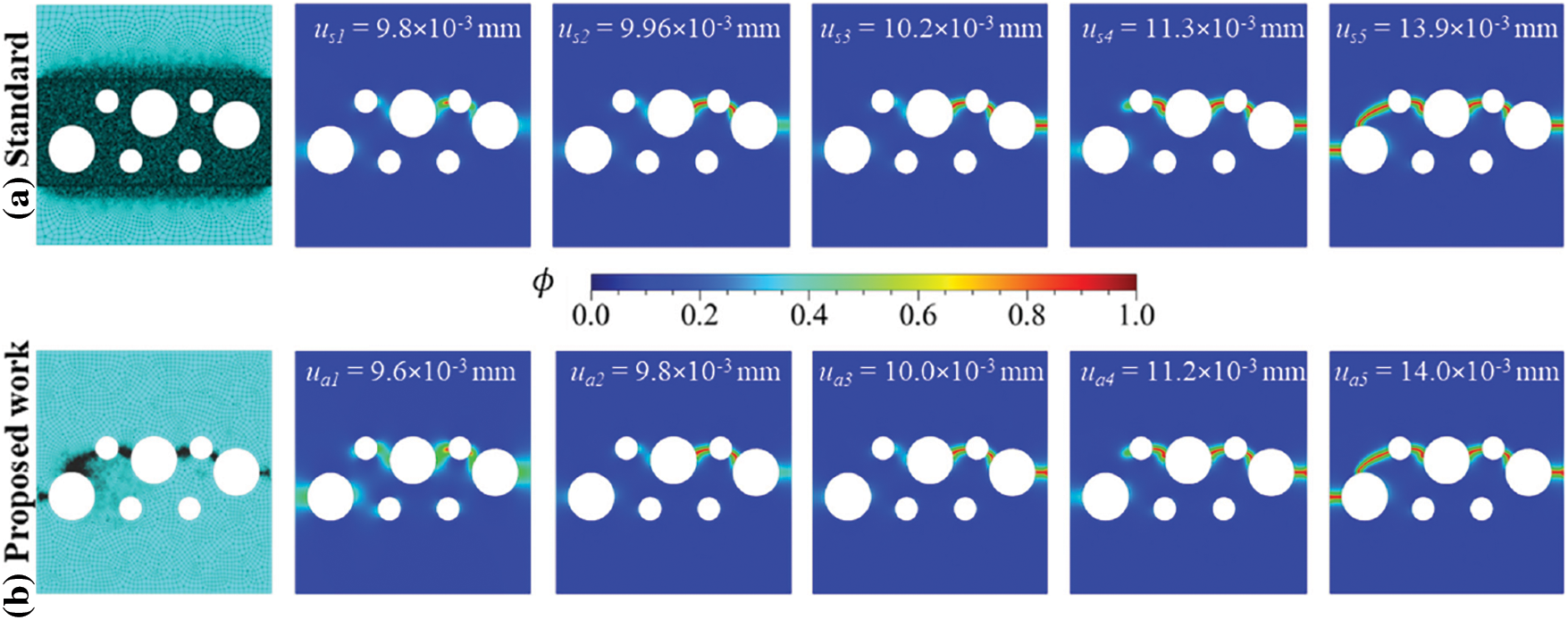
Figure 26: Discretized specimen and phase-field contours for (a) Standard PFM and (b) Proposed PFM implementation for square plate with 7 holes at l0 = 0.008 mm

The specimen is initially discretized for the proposed PFM implementation with a global element size of 0.02 mm. The initial ‘Job-1.inp’ file obtains the nodal coordinates and element connectivity for the initial UEL job ‘Job-1_UEL.inp’. The initial UEL job provides corresponding MISESERI values on an element basis, as shown in Fig. 25b. The MISESERI values can potentially predict the region for local mesh refinement positively. The remeshing rule enforces a local refinement with mesh size, h = 0.001 mm, and global mesh size 0.03 mm, as shown in Fig. 26b. The increment size for ‘Job-1_UEL.inp’ is considered as Δu1 = 10−5 for 3100 increments and then Δu2 = 5 × 10−6 for further 4500 increments, whereas the increment size for the post-adaptive refinement job ‘Job-2_UEL.inp’ is considered the same as that of standard PFM.

The phase field contours for the proposed PFM are shown in Fig. 26b, corresponding to the points marked in Fig. 27a. The crack trajectory obtained using the proposed PFM is qualitatively in agreement with the standard PFM results and those reported in the literature [106]. The structural response for standard and proposed PFM is found to be similar and shown in Fig. 27a. Further, a comparative analysis of the computational efficiency of standard PFM and proposed PFM is presented in Fig. 27b. The proposed PFM takes 555 min, while the standard PFM takes 1942 min to analyze the problem. The order of AMATRX for standard PFM is more than five times that of the proposed PFM, which signifies that the latter also provides huge savings in memory requirement.

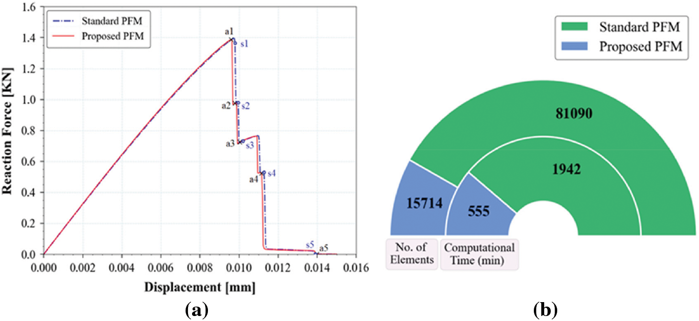
Figure 27: (a) Load-displacement response for a square plate specimen with 7 holes, (b) Computational time and number of elements comparison metrics between standard PFM and proposed PFM for a square plate specimen with 7 holes

5  Conclusion

This work discusses the implementation procedure of the posteriori error indicator-based mesh refinement algorithm for the phase field model in Abaqus. The proposed algorithm implementation in PFM is executed in Abaqus using a Python script that features user-defined functions/procedures for the operational plan. The robustness and efficiency of the proposed approach are examined through several standard fracture problems. The proposed study is performed within the small-strain framework, utilizing the AT-2 phase-field brittle fracture formulation in the 2D domain. The material behavior is assumed to be linear elastic with anisotropic degradation, enabling the dissociation of tensile and compressive fields via the spectral split of the strain tensor contributing to the strain energy functional. The history variable approach is used to enforce fracture irreversibility. The algorithm, at present, does not incorporate dynamic effects, multi-physics coupling, such as thermomechanical interactions, etc. To focus on the efficacy of the mesh refinement strategy and developing a basic framework, simplified geometries and boundary conditions with different fracture nucleation scenarios—presence/absence of a physical notch, multiple voids in the specimen, mixed mode fracture, etc., are considered as examples. As the refinement strategy involves Abaqus’ built-in error indicator, a few case studies investigating the sensitivity of key parameters, including the length scale parameter, initial coarse mesh size, and Remeshing Rule arguments (errorTarget, refinementFactor), are presented. While the extension to 3D geometries seems to be an encouraging and practical direction, it is currently beyond the scope of this study due to added complexity and computational demands. However, it remains a significant motivation for our future work with enhancements such as incorporating the restart analysis-based simulations, integrated with explicit solution schemes and parallelization features of the Abaqus utility. The conclusions drawn, based on the study, are given as:

•   The proposed algorithm in the PFM approach enables Abaqus’ built-in error indicators to be used for mesh refinement instead of user-specified computations at the element level to mark regions requiring local mesh pre-refinement.

•   The proposed approach successfully captures the expected crack path through the Abaqus built-in MISESERI indicator.

•   The proposed PFM approach eliminates the requirement to designate a high mesh density zone based on prior information about the crack growth direction. Hence, the proposed approach can be used to solve more generic problems.

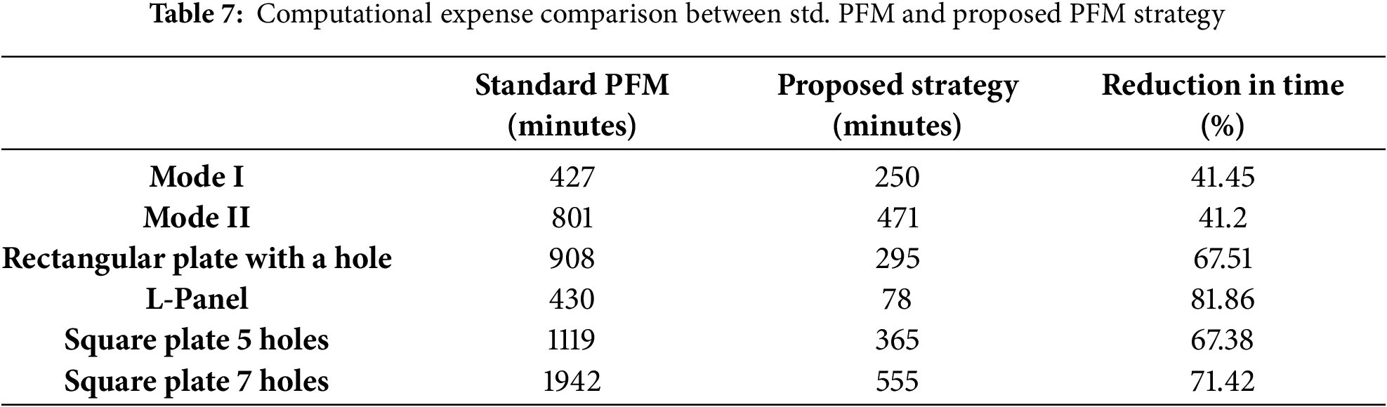
•   The proposed PFM can provide accurate results with significantly reduced computational resource requirements. For mode I and mode II problems, the proposed approach produces sufficiently accurate results with approximately 41% lower computational costs than the standard PFM implementation. For the rest of the benchmark numerical problems, resource savings in the range of 67%–82% are achieved (Table 7).

•   Although the proposed PFM performance and capability are positively demonstrated for 2D problems, extension to 3D problems is a potential future work to be considered.

Acknowledgement: The authors have not received any funding for this work. However, they acknowledge the Indian Institute of Technology Ropar for providing the necessary facilities used in this study.

Funding Statement: The authors received no specific funding for this study.

Author Contributions: The authors confirm contribution to the paper as follows—Anshul Pandey: conception and design of study, methodology, acquisition of data, analysis and/or interpretation of data, writing. Sachin Kumar: supervision, conception and design of study, analysis and/or interpretation of data, drafting the manuscript, writing—review & editing. All authors reviewed the results and approved the final version of the manuscript.

Availability of Data and Materials: The necessary data will be made available on request from the authors.

Ethics Approval: Not Applicable: The present study did not involve any human or animal participants.

Conflicts of Interest: The authors declare no conflicts of interest to report regarding the present study.

References

1. Griffiths AA.VI. The phenomena of rupture and flow in solids. Philos Trans R Soc Lond Ser A Contain Pap Math Phys Character. 1921;221:163–98. doi:10.1098/rsta.1921.0006. [Google Scholar] [CrossRef]

2. Irwin GR. Analysis of stresses and strains near the end of a crack traversing a plate. J Appl Mech. 1957;24(3):361–4. doi:10.1115/1.4011547. [Google Scholar] [CrossRef]

3. Barenblatt GI. The mathematical theory of equilibrium cracks in brittle fracture. In: Advances in applied mechanics. Vol. 7. Amsterdam: Elsevier; 1962. p. 55–129. doi:10.1016/s0065-2156(08)70121-2. [Google Scholar] [CrossRef]

4. Dugdale DS. Yielding of steel sheets containing slits. J Mech Phys Solids. 1960;8(2):100–4. doi:10.1016/0022-5096(60)90013-2. [Google Scholar] [CrossRef]

5. Belytschko T. The finite element method: linear static and dynamic finite element analysis. Thomas J R Hughes Comput Aided Civ Infrastruct Eng. 1989;4(3):245–6. doi:10.1111/j.1467-8667.1989.tb00025.x. [Google Scholar] [CrossRef]

6. Belytschko T, Gu L, Lu YY. Fracture and crack growth by element free Galerkin methods. Modelling Simul Mater Sci Eng. 1994;2(3A):519–34. doi:10.1088/0965-0393/2/3a/007. [Google Scholar] [CrossRef]

7. Pathak H, Singh A, Singh IV. Numerical simulation of bi-material interfacial cracks using EFGM and XFEM. Int J Mech Mater Des. 2012;8(1):9–36. doi:10.1007/s10999-011-9173-3. [Google Scholar] [CrossRef]

8. Belytschko T, Black T. Elastic crack growth in finite elements with minimal remeshing. Int J Numer Meth Eng. 1999;45(5):601–20. [Google Scholar]

9. Kumar S, Singh IV, Mishra BK, Rabczuk T. Modeling and simulation of kinked cracks by virtual node XFEM. Comput Meth Appl Mech Eng. 2015;283:1425–66. doi:10.1016/j.cma.2014.10.019. [Google Scholar] [CrossRef]

10. Kumar S, Wang Y, Poh LH, Chen B. Floating node method with domain-based interaction integral for generic 2D crack growths. Theor Appl Fract Mech. 2018;96:483–96. doi:10.1016/j.tafmec.2018.06.013. [Google Scholar] [CrossRef]

11. Singh U, Kumar S, Chen B. Smoothed floating node method for modelling 2D arbitrary crack propagation problems. Theor Appl Fract Mech. 2022;117:103190. doi:10.1016/j.tafmec.2021.103190. [Google Scholar] [CrossRef]

12. Hughes TJR, Cottrell JA, Bazilevs Y. Isogeometric analysis: cad, finite elements, NURBS, exact geometry and mesh refinement. Comput Meth Appl Mech Eng. 2005;194(39–41):4135–95. doi:10.1016/j.cma.2004.10.008. [Google Scholar] [CrossRef]

13. Soni A, Negi A, Kumar S, Kumar N. An IGA based nonlocal gradient-enhanced damage model for failure analysis of cortical bone. Eng Fract Mech. 2021;255(2):107976. doi:10.1016/j.engfracmech.2021.107976. [Google Scholar] [CrossRef]

14. Feng Z, Duan Q, Chen S. Adaptive phantom node method: an efficient and robust approach towards complex engineering cracks. Eng Anal Bound Elem. 2023;156(9):356–71. doi:10.1016/j.enganabound.2023.08.013. [Google Scholar] [CrossRef]

15. Rabczuk T, Belytschko T. Cracking particles: a simplified meshfree method for arbitrary evolving cracks. Int J Numer Meth Eng. 2004;61(13):2316–43. doi:10.1002/nme.1151. [Google Scholar] [CrossRef]

16. Rabczuk T, Zi G, Bordas S, Nguyen-Xuan H. A simple and robust three-dimensional cracking-particle method without enrichment. Comput Meth Appl Mech Eng. 2010;199(37–40):2437–55. doi:10.1016/j.cma.2010.03.031. [Google Scholar] [CrossRef]

17. Silling SA. Reformulation of elasticity theory for discontinuities and long-range forces. J Mech Phys Solids. 2000;48(1):175–209. doi:10.1016/s0022-5096(99)00029-0. [Google Scholar] [CrossRef]

18. Silling SA, Epton M, Weckner O, Xu J, Askari E. Peridynamic states and constitutive modeling. J Elast. 2007;88(2):151–84. doi:10.1007/s10659-007-9125-1. [Google Scholar] [CrossRef]

19. Ni T, Zaccariotto M, Zhu QZ, Galvanetto U. Coupling of FEM and ordinary state-based peridynamics for brittle failure analysis in 3D. Mech Adv Mater Struct. 2021;28(9):875–90. doi:10.1080/15376494.2019.1602237. [Google Scholar] [CrossRef]

20. Kachanov LM. Rupture time under creep conditions. Int J Fract. 1999;97(1):11–8. doi:10.1023/A:1018671022008. [Google Scholar] [CrossRef]

21. Jirásek M. Mathematical analysis of strain localization. Rev Eur De Génie Civ. 2007;11(7–8):977–91. doi:10.1080/17747120.2007.9692973. [Google Scholar] [CrossRef]

22. Karma A, Kessler DA, Levine H. Phase-field model of mode III dynamic fracture. Phys Rev Lett. 2001;87(4):045501. doi:10.1103/PhysRevLett.87.045501. [Google Scholar] [PubMed] [CrossRef]

23. Hakim V, Karma A. Laws of crack motion and phase-field models of fracture. J Mech Phys Solids. 2009;57(2):342–68. doi:10.1016/j.jmps.2008.10.012. [Google Scholar] [CrossRef]

24. Francfort GA, Marigo JJ. Revisiting brittle fracture as an energy minimization problem. J Mech Phys Solids. 1998;46(8):1319–42. doi:10.1016/s0022-5096(98)00034-9. [Google Scholar] [CrossRef]

25. Mumford D, Shah J. Optimal approximations by piecewise smooth functions and associated variational problems. Commun Pure Appl Math. 1989;42(5):577–685. doi:10.1002/cpa.3160420503. [Google Scholar] [CrossRef]

26. Buliga M. Energy minimizing brittle crack propagation. J Elast. 1998;52(3):201–38. doi:10.1023/A:1007545213010. [Google Scholar] [CrossRef]

27. Bourdin B, Francfort GA, Marigo JJ. Numerical experiments in revisited brittle fracture. J Mech Phys Solids. 2000;48(4):797–826. doi:10.1016/s0022-5096(99)00028-9. [Google Scholar] [CrossRef]

28. Bourdin B. Numerical implementation of the variational formulation for quasi-static brittle fracture. Interfaces Free Bound. 2007;9(3):411–30. doi:10.4171/ifb/171. [Google Scholar] [CrossRef]

29. Francfort GA, Bourdin B, Marigo JJ. The variational approach to fracture. J Elast. 2008;91(1):5–148. doi:10.1007/s10659-007-9107-3. [Google Scholar] [CrossRef]

30. Amor H, Marigo JJ, Maurini C. Regularized formulation of the variational brittle fracture with unilateral contact: numerical experiments. J Mech Phys Solids. 2009;57(8):1209–29. doi:10.1016/j.jmps.2009.04.011. [Google Scholar] [CrossRef]

31. Lancioni G, Royer-Carfagni G. The variational approach to fracture mechanics. A practical application to the French panthéon in Paris. J Elast. 2009;95(1):1–30. doi:10.1007/s10659-009-9189-1. [Google Scholar] [CrossRef]

32. Miehe C, Welschinger F, Hofacker M. Thermodynamically consistent phase-field models of fracture: variational principles and multi-field FE implementations. Int J Numer Meth Eng. 2010;83(10):1273–311. doi:10.1002/nme.2861. [Google Scholar] [CrossRef]

33. Wu JY, Cervera M. A novel positive/negative projection in energy norm for the damage modeling of quasi-brittle solids. Int J Solids Struct. 2018;139–140(10):250–69. doi:10.1016/j.ijsolstr.2018.02.004. [Google Scholar] [CrossRef]

34. Wu JY, Nguyen VP. A length scale insensitive phase-field damage model for brittle fracture. J Mech Phys Solids. 2018;119(8):20–42. doi:10.1016/j.jmps.2018.06.006. [Google Scholar] [CrossRef]

35. Kriaa Y, Hentati H, Zouari B. Applying the phase-field approach for brittle fracture prediction: numerical implementation and experimental validation. Mech Adv Mater Struct. 2022;29(6):828–39. doi:10.1080/15376494.2020.1795957. [Google Scholar] [CrossRef]

36. Dujc J, Brank B. Combining coupled, staggered and uncoupled solution methods for phase-field-based fracture analysis. Mech Adv Mater Struct. 2022;29(27):6361–78. doi:10.1080/15376494.2021.1976888. [Google Scholar] [CrossRef]

37. Wu JY, Huang Y. Comprehensive implementations of phase-field damage models in Abaqus. Theor Appl Fract Mech. 2020;106(4):102440. doi:10.1016/j.tafmec.2019.102440. [Google Scholar] [CrossRef]

38. Yu Y, Hou C, Zheng X, Rabczuk T, Zhao M. An efficient and robust staggered scheme based on adaptive time field for phase field fracture model. Eng Fract Mech. 2024;301(7–8):110025. doi:10.1016/j.engfracmech.2024.110025. [Google Scholar] [CrossRef]

39. Ambati M, Gerasimov T, De Lorenzis L. A review on phase-field models of brittle fracture and a new fast hybrid formulation. Comput Mech. 2015;55(2):383–405. doi:10.1007/s00466-014-1109-y. [Google Scholar] [CrossRef]

40. Wu JY, Nguyen VP, Nguyen CT, Sutula D, Sinaie S, Bordas SPA. Phase-field modeling of fracture. In: Advances in applied mechanics. Amsterdam: Elsevier; 2020. p. 1–183. doi:10.1016/bs.aams.2019.08.001. [Google Scholar] [CrossRef]

41. Miehe C, Hofacker M, Welschinger F. A phase field model for rate-independent crack propagation: robust algorithmic implementation based on operator splits. Comput Meth Appl Mech Eng. 2010;199(45–48):2765–78. doi:10.1016/j.cma.2010.04.011. [Google Scholar] [CrossRef]

42. Loew PJ, Peters B, Beex LAA. Rate-dependent phase-field damage modeling of rubber and its experimental parameter identification. J Mech Phys Solids. 2019;127(8):266–94. doi:10.1016/j.jmps.2019.03.022. [Google Scholar] [CrossRef]

43. Huber W, Asle Zaeem M. A mixed mode phase-field model of ductile fracture. J Mech Phys Solids. 2023;171(4):105123. doi:10.1016/j.jmps.2022.105123. [Google Scholar] [CrossRef]

44. Ulloa J, Wambacq J, Alessi R, Samaniego E, Degrande G, François S. A micromechanics-based variational phase-field model for fracture in geomaterials with brittle-tensile and compressive-ductile behavior. J Mech Phys Solids. 2022;159:104684. doi:10.1016/j.jmps.2021.104684. [Google Scholar] [CrossRef]

45. Mandal TK, Gupta A, Nguyen VP, Chowdhury R, de Vaucorbeil A. A length scale insensitive phase field model for brittle fracture of hyperelastic solids. Eng Fract Mech. 2020;236(4):107196. doi:10.1016/j.engfracmech.2020.107196. [Google Scholar] [CrossRef]

46. Mandal TK, Nguyen VP, Wu JY. A length scale insensitive anisotropic phase field fracture model for hyperelastic composites. Int J Mech Sci. 2020;188(8):105941. doi:10.1016/j.ijmecsci.2020.105941. [Google Scholar] [CrossRef]

47. Paggi M, Corrado M, Reinoso J. Fracture of solar-grade anisotropic polycrystalline silicon: a combined phase field-cohesive zone model approach. Comput Meth Appl Mech Eng. 2018;330(5):123–48. doi:10.1016/j.cma.2017.10.021. [Google Scholar] [CrossRef]

48. Zhu J, Luo J. Study of transformation induced intergranular microcracking in tetragonal zirconia polycrystals with the phase field method. Mater Sci Eng A. 2017;701(5):69–84. doi:10.1016/j.msea.2017.06.060. [Google Scholar] [CrossRef]

49. Nguyen-Thanh N, Nguyen-Xuan H, Li W. Phase-field modeling of anisotropic brittle fracture in rock-like materials and polycrystalline materials. Comput Struct. 2024;296(11):107325. doi:10.1016/j.compstruc.2024.107325. [Google Scholar] [CrossRef]

50. Kiran R, Nguyen-Thanh N, Zhou K. Adaptive isogeometric analysis-based phase-field modeling of brittle electromechanical fracture in piezoceramics. Eng Fract Mech. 2022;274(45–48):108738. doi:10.1016/j.engfracmech.2022.108738. [Google Scholar] [CrossRef]

51. Simoes M, Martínez-Pañeda E. Phase field modelling of fracture and fatigue in Shape Memory Alloys. Comput Meth Appl Mech Eng. 2021;373(96):113504. doi:10.1016/j.cma.2020.113504. [Google Scholar] [CrossRef]

52. Simoes M, Braithwaite C, Makaya A, Martínez-Pañeda E. Modelling fatigue crack growth in shape memory alloys. Fatigue Fract Eng Mater Struct. 2022;45(4):1243–57. doi:10.1111/ffe.13638. [Google Scholar] [CrossRef]

53. Zhang B, Luo J, Fang Z, Huang H. Phase field study of the thermo-electro-mechanical fracture behavior of flexoelectric solids. Theor Appl Fract Mech. 2023;125:103833. doi:10.1016/j.tafmec.2023.103833. [Google Scholar] [CrossRef]

54. Li H, Yu T, Liu Z, Sun J, Chen L. Adaptive phase-field modeling for electromechanical fracture in flexoelectric materials using multi-patch isogeometric analysis. Comput Meth Appl Mech Eng. 2025;443(6):118070. doi:10.1016/j.cma.2025.118070. [Google Scholar] [CrossRef]

55. Xia X, Qin C, Lu G, Gu X, Zhang Q. Simulation of corrosion-induced cracking of reinforced concrete based on fracture phase field method. Comput Model Eng Sci. 2024;138(3):2257–76. doi:10.32604/cmes.2023.031238. [Google Scholar] [CrossRef]

56. Farrell P, Maurini C. Linear and nonlinear solvers for variational phase-field models of brittle fracture. Int J Numer Meth Eng. 2017;109(5):648–67. doi:10.1002/nme.5300. [Google Scholar] [CrossRef]

57. Barchiesi E, Yang H, Tran CA, Placidi L, Müller WH. Computation of brittle fracture propagation in strain gradient materials by the FEniCS library. Math Mech Solids. 2021;26(3):325–40. doi:10.1177/1081286520954513. [Google Scholar] [CrossRef]

58. Tangella RG, Kumbhar P, Annabattula RK. Hybrid phase field modelling of dynamic brittle fracture and implementation in FEniCS. In: Composite materials for extreme loading. Singapore: Springer; 2021. p. 15–24. doi:10.1007/978-981-16-4138-1_2. [Google Scholar] [CrossRef]

59. May S, Vignollet J, de Borst R. A numerical assessment of phase-field models for brittle and cohesive fracture: Γ-Convergence and stress oscillations. Eur J Mech A. 2015;52:72–84. doi:10.1016/j.euromechsol.2015.02.002. [Google Scholar] [CrossRef]

60. Ahmed A, Khan R. A phase field model for damage in asphalt concrete. Int J Pavement Eng. 2022;23(12):4320–32. doi:10.1080/10298436.2021.1942871. [Google Scholar] [CrossRef]

61. Freddi F, Mingazzi L. Adaptive mesh refinement for the phase field method: a FEniCS implementation. Appl Eng Sci. 2023;14(2):100127. doi:10.1016/j.apples.2023.100127. [Google Scholar] [CrossRef]

62. Patil RU, Mishra BK, Singh IV. An adaptive multiscale phase field method for brittle fracture. Comput Meth Appl Mech Eng. 2018;329(4):254–88. doi:10.1016/j.cma.2017.09.021. [Google Scholar] [CrossRef]

63. Hirshikesh, Jansari C, Kannan K, Annabattula RK, Natarajan S. Adaptive phase field method for quasi-static brittle fracture using a recovery based error indicator and quadtree decomposition. Eng Fract Mech. 2019;220:106599. doi:10.1016/j.engfracmech.2019.106599. [Google Scholar] [CrossRef]

64. Klinsmann M, Rosato D, Kamlah M, McMeeking RM. An assessment of the phase field formulation for crack growth. Comput Meth Appl Mech Eng. 2015;294(10):313–30. doi:10.1016/j.cma.2015.06.009. [Google Scholar] [CrossRef]

65. Jin T, Li Z, Chen K. A novel phase-field monolithic scheme for brittle crack propagation based on the limited-memory BFGS method with adaptive mesh refinement. Int J Numer Meth Eng. 2024;125(22):e7572. doi:10.1002/nme.7572. [Google Scholar] [CrossRef]

66. Gaston D, Newman C, Hansen G, Lebrun-Grandié D. MOOSE: a parallel computational framework for coupled systems of nonlinear equations. Nucl Eng Des. 2009;239(10):1768–78. doi:10.1016/j.nucengdes.2009.05.021. [Google Scholar] [CrossRef]

67. Ghaffari Motlagh Y, Jimack PK, de Borst R. Deep learning phase-field model for brittle fractures. Int J Numer Meth Eng. 2023;124(3):620–38. doi:10.1002/nme.7135. [Google Scholar] [CrossRef]

68. Samaniego E, Anitescu C, Goswami S, Nguyen-Thanh VM, Guo H, Hamdia K, et al. An energy approach to the solution of partial differential equations in computational mechanics via machine learning: concepts, implementation and applications. Comput Meth Appl Mech Eng. 2020;362(2):112790. doi:10.1016/j.cma.2019.112790. [Google Scholar] [CrossRef]

69. Goswami S, Anitescu C, Chakraborty S, Rabczuk T. Transfer learning enhanced physics informed neural network for phase-field modeling of fracture. Theor Appl Fract Mech. 2020;106:102447. doi:10.1016/j.tafmec.2019.102447. [Google Scholar] [CrossRef]

70. Wu JY, Huang Y, Nguyen VP. On the BFGS monolithic algorithm for the unified phase field damage theory. Comput Meth Appl Mech Eng. 2020;360(8):112704. doi:10.1016/j.cma.2019.112704. [Google Scholar] [CrossRef]

71. Msekh MA, Sargado JM, Jamshidian M, Areias PM, Rabczuk T. Abaqus implementation of phase-field model for brittle fracture. Comput Mater Sci. 2015;96(8):472–84. doi:10.1016/j.commatsci.2014.05.071. [Google Scholar] [CrossRef]

72. Molnár G, Gravouil A. 2D and 3D Abaqus implementation of a robust staggered phase-field solution for modeling brittle fracture. Finite Elem Anal Des. 2017;130(582–593):27–38. doi:10.1016/j.finel.2017.03.002. [Google Scholar] [CrossRef]

73. Navidtehrani Y, Betegón C, Martínez-Pañeda E. A simple and robust Abaqus implementation of the phase field fracture method. Appl Eng Sci. 2021;6(12):100050. doi:10.1016/j.apples.2021.100050. [Google Scholar] [CrossRef]

74. Liu G, Li Q, Msekh MA, Zuo Z. Abaqus implementation of monolithic and staggered schemes for quasi-static and dynamic fracture phase-field model. Comput Mater Sci. 2016;121(4):35–47. doi:10.1016/j.commatsci.2016.04.009. [Google Scholar] [CrossRef]

75. Pillai U, Heider Y, Markert B. A diffusive dynamic brittle fracture model for heterogeneous solids and porous materials with implementation using a user-element subroutine. Comput Mater Sci. 2018;153(5):36–47. doi:10.1016/j.commatsci.2018.06.024. [Google Scholar] [CrossRef]

76. Jeong H, Signetti S, Han TS, Ryu S. Phase field modeling of crack propagation under combined shear and tensile loading with hybrid formulation. Comput Mater Sci. 2018;155:483–92. doi:10.1016/j.commatsci.2018.09.021. [Google Scholar] [CrossRef]

77. Reddy SSK, Amirtham R, Reddy JN. Modeling fracture in brittle materials with inertia effects using the phase field method. Mech Adv Mater Struct. 2023;30(1):144–59. doi:10.1080/15376494.2021.2010289. [Google Scholar] [CrossRef]

78. Hu X, Tan S, Xia D, Min L, Xu H, Yao W, et al. An overview of implicit and explicit phase field models for quasi-static failure processes, implementation and computational efficiency. Theor Appl Fract Mech. 2023;124(2):103779. doi:10.1016/j.tafmec.2023.103779. [Google Scholar] [CrossRef]

79. Kristensen PK, Martínez-Pañeda E. Phase field fracture modelling using quasi-Newton methods and a new adaptive step scheme. Theor Appl Fract Mech. 2020;107(8):102446. doi:10.1016/j.tafmec.2019.102446. [Google Scholar] [CrossRef]

80. Bharali R, Goswami S, Anitescu C, Rabczuk T. A robust monolithic solver for phase-field fracture integrated with fracture energy based arc-length method and under-relaxation. Comput Meth Appl Mech Eng. 2022;394(8):114927. doi:10.1016/j.cma.2022.114927. [Google Scholar] [CrossRef]

81. Singh N, Verhoosel CV, de Borst R, van Brummelen EH. A fracture-controlled path-following technique for phase-field modeling of brittle fracture. Finite Elem Anal Des. 2016;113(45–48):14–29. doi:10.1016/j.finel.2015.12.005. [Google Scholar] [CrossRef]

82. Zhang P, Yao W, Hu X, Bui TQ. An explicit phase field model for progressive tensile failure of composites. Eng Fract Mech. 2021;241:107371. doi:10.1016/j.engfracmech.2020.107371. [Google Scholar] [CrossRef]

83. Su XT, Yang ZJ, Liu GH. Monte Carlo simulation of complex cohesive fracture in random heterogeneous quasi-brittle materials: a 3D study. Int J Solids Struct. 2010;47(17):2336–45. doi:10.1016/j.ijsolstr.2010.04.031. [Google Scholar] [CrossRef]

84. Hai L, Li J. A rate-dependent phase-field framework for the dynamic failure of quasi-brittle materials. Eng Fract Mech. 2021;252(2):107847. doi:10.1016/j.engfracmech.2021.107847. [Google Scholar] [CrossRef]

85. Martínez-Pañeda E, Golahmar A, Niordson CF. A phase field formulation for hydrogen assisted cracking. Comput Meth Appl Mech Eng. 2018;342(3):742–61. doi:10.1016/j.cma.2018.07.021. [Google Scholar] [CrossRef]

86. Gupta A, Krishnan UM, Chowdhury R, Chakrabarti A. An auto-adaptive sub-stepping algorithm for phase-field modeling of brittle fracture. Theor Appl Fract Mech. 2020;108(4):102622. doi:10.1016/j.tafmec.2020.102622. [Google Scholar] [CrossRef]

87. Saberi H, Saberi H, Quoc Bui T, Heider Y, Ngoc Nguyen M. A multi-level adaptive mesh refinement method for phase-field fracture problems. Theor Appl Fract Mech. 2023;125(12):103920. doi:10.1016/j.tafmec.2023.103920. [Google Scholar] [CrossRef]

88. Dean A, Asur Vijaya Kumar PK, Reinoso J, Gerendt C, Paggi M, Mahdi E, et al. A multi phase-field fracture model for long fiber reinforced composites based on the Puck theory of failure. Compos Struct. 2020;251:112446. doi:10.1016/j.compstruct.2020.112446. [Google Scholar] [CrossRef]

89. Freddi F, Mingazzi L. Mesh refinement procedures for the phase field approach to brittle fracture. Comput Meth Appl Mech Eng. 2022;388(8):114214. doi:10.1016/j.cma.2021.114214. [Google Scholar] [CrossRef]

90. Schlüter A, Willenbücher A, Kuhn C, Müller R. Phase field approximation of dynamic brittle fracture. Comput Mech. 2014;54(5):1141–61. doi:10.1007/s00466-014-1045-x. [Google Scholar] [CrossRef]

91. Paul K, Zimmermann C, Mandadapu KK, Hughes TJR, Landis CM, Sauer RA. An adaptive space-time phase field formulation for dynamic fracture of brittle shells based on LR NURBS. Comput Mech. 2020;65(4):1039–62. doi:10.1007/s00466-019-01807-y. [Google Scholar] [CrossRef]

92. Tian F, Tang X, Xu T, Yang J, Li L. A hybrid adaptive finite element phase-field method for quasi-static and dynamic brittle fracture. Int J Numer Meth Eng. 2019;120(9):1108–25. doi:10.1002/nme.6172. [Google Scholar] [CrossRef]

93. Li T, Marigo JJ, Guilbaud D, Potapov S. Gradient damage modeling of brittle fracture in an explicit dynamics context. Int J Numer Meth Eng. 2016;108(11):1381–405. doi:10.1002/nme.5262. [Google Scholar] [CrossRef]

94. Mahnken R. Goal-oriented adaptive refinement for phase field modeling with finite elements. Int J Numer Meth Eng. 2013;94(4):418–40. doi:10.1002/nme.4464. [Google Scholar] [CrossRef]

95. Hirshikesh, Pramod ALN, Annabattula RK, Ooi ET, Song C, Natarajan S. Adaptive phase-field modeling of brittle fracture using the scaled boundary finite element method. Comput Meth Appl Mech Eng. 2019;355:284–307. doi:10.1016/j.cma.2019.06.002. [Google Scholar] [CrossRef]

96. Wick T. Goal functional evaluations for phase-field fracture using PU-based DWR mesh adaptivity. Comput Mech. 2016;57(6):1017–35. doi:10.1007/s00466-016-1275-1. [Google Scholar] [CrossRef]

97. Pandey A, Kumar S. A multi-level adaptive mesh refinement strategy for unified phase field fracture modeling using unstructured conformal simplices. Comput Meth Appl Mech Eng. 2025;433:117514. doi:10.1016/j.cma.2024.117514. [Google Scholar] [CrossRef]

98. Huang YJ, Zheng ZS, Yao F, Zeng C, Zhang H, Natarajan S, et al. Arbitrary polygon-based CSFEM-PFCZM for quasi-brittle fracture of concrete. Comput Meth Appl Mech Eng. 2024;424(3):116899. doi:10.1016/j.cma.2024.116899. [Google Scholar] [CrossRef]

99. Wu JY. A unified phase-field theory for the mechanics of damage and quasi-brittle failure. J Mech Phys Solids. 2017;103(4):72–99. doi:10.1016/j.jmps.2017.03.015. [Google Scholar] [CrossRef]

100. Ambrosio L, Tortorelli VM. Approximation of functional depending on jumps by elliptic functional via t-convergence. Commun Pure Appl Math. 1990;43(8):999–1036. doi:10.1002/cpa.3160430805. [Google Scholar] [CrossRef]

101. Zienkiewicz OC, Zhu JZ. The superconvergent patch recovery and a posteriori error estimates. Part 1: the recovery technique. Int J Numer Meth Eng. 1992;33(7):1331–64. doi:10.1002/nme.1620330702. [Google Scholar] [CrossRef]

102. Zienkiewicz OC, Zhu JZ. A simple error estimator and adaptive procedure for practical engineerng analysis. Int J Numer Meth Eng. 1987;24(2):337–57. doi:10.1002/nme.1620240206. [Google Scholar] [CrossRef]

103. Zienkiewicz OC, Zhu JZ. The superconvergent patch recovery and a posteriori error estimates. Part 2: error estimates and adaptivity. Int J Numer Meth Eng. 1992;33(7):1365–82. doi:10.1002/nme.1620330703. [Google Scholar] [CrossRef]

104. Winkler B, Hofstetter G, Niederwanger G. Experimental verification of a constitutive model for concrete cracking. Proc Inst Mech Eng Part L J Mater Des Appl. 2001;215(2):75–86. doi:10.1177/146442070121500202. [Google Scholar] [CrossRef]

105. Lampron O, Therriault D, Lévesque M. An efficient and robust monolithic approach to phase-field quasi-static brittle fracture using a modified Newton method. Comput Meth Appl Mech Eng. 2021;386(582–593):114091. doi:10.1016/j.cma.2021.114091. [Google Scholar] [CrossRef]

106. Han J, Shintaku Y, Moriguchi S, Terada K. A transition scheme from diffusive to discrete crack topologies at finite strain during the course of a staggered iterative procedure. Int J Numer Meth Eng. 2023;124(6):1405–33. doi:10.1002/nme.7169. [Google Scholar] [CrossRef]