Topology Optimization of Lattice Structures through Data-Driven Model of M-VCUT Level Set Based Substructure

1  Introduction

Lattice structures have excellent mechanical properties, for instance, the high specific strength and stiffness, and their rich geometric characteristics give a large design space [1]. Therefore, it is used in various engineering applications [2–4].

Because many microscale features exist in the lattice structures, an accurate finite element analysis (FEA) calls for a fine mesh to capture their mechanical behavior, and this is time-consuming [5]. To improve the computational efficiency of FEA and sensitivity analysis in the topology optimization of lattice structures, scholars often use homogenization to obtain the effective properties of microscale features and view them as homogeneous materials [6–10]. In addition to compliance problem [11–13], scholars have also done a lot of work in other fields such as stress constraint [14–16]. The use of homogenization, however, requires two conditions to be met: (1) the microstructures should be periodically distributed; (2) the scale of the microstructure should be much smaller than that of the macrostructure. However, the two conditions can not be strictly satisfied in many engineering applications. In such circumstances, to improve the computational efficiency, the extended multiscale finite element method [17–19] and substructure method [20–24] are often used.

In the present study on the topology optimization of lattice structures, the substructure method is also used. The lattice structure is divided into multiple substructures. Each substructure is converted to a super element through static condensation that retains only the boundary nodes. By this means, the degrees of freedom of the stiffness matrix is reduced [24]. The key ideas of the present study is explained as follows.

First, the M-VCUT level set method is used to generate substructures with various configurations [25–27], and this diversity of configuration is important for obtaining a large design space of topology optimization. In addition, the M-VCUT level set method also ensures the connectivity between neighboring substructures [26].

Second, in order to avoid time-consuming static condensation once the configurations of substructures are changed during the optimization, a data-driven model is constructed. In an offline stage, a database is prepared by sampling the space of substructures spanned by several prototypes of substructures, and for each substructure in this database, static condensation is used to obtain its stiffness matrix. Meanwhile, the volume of the substructure is also computed. Then, a data-driven model of substructures is constructed through interpolation with CS-RBF [28–30]. The inputs of the data-driven model are the design variables of topology optimization, and the outputs are the condensed stiffness matrix and volume of substructures. In the online optimization stage, this data-driven model is used in the FEA and sensitivity analysis.

The remaining part of this paper is organized as follows. Section 2 introduces the representation of lattice structures and substructures. Section 3 introduces the data-driven model. Section 4 presents the optimization problem and sensitivity analysis. Section 5 presents several examples of topology optimization. The conclusion is presented in Section 6.

2  Geometric and Mechanical Models of Substructure

The geometry of substructure is modeled by using the M-VCUT level set method [25,26]. The mechanical model of substructures, i.e., the stiffness matrix in the present study, is obtained by static condensation [20,21].

2.1 Geometry Model of Substructure Based on M-VCUT Level Set

In the optimization, the lattice structure Ω⊂Rd (where d=2 or 3) is confined within a reference domain D⊂Rd, i.e., Ω⊂D. According to the substructure method, D is divided into cells Dk so that D=⋃k=1MDk, as shown in Fig. 1. Within each cell Dk, a substructure Ωk may exist, i.e., Ωk⊂Dk. Therefore, the lattice structure Ω can be represented by the assembly of substructures as

Ω=∪k=1MΩk(1)

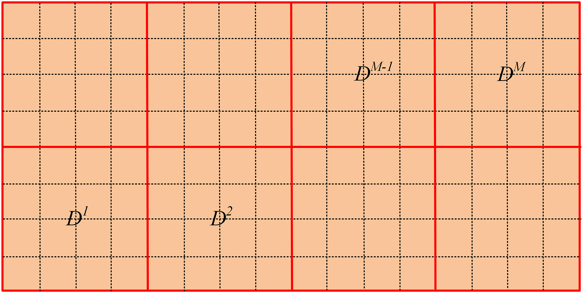
Figure 1: Design domain of lattice structure is divided into multiple cells

According to the M-VCUT level set method, a substructure Ωk in Dk is described by using N pairs of basic level set functions Φi(x) and a cutting height plane hi, i=1,...,N. Each Φi is cut by its corresponding hi, and after completing the cutting operations, N virtual substructure Ω~i are obtained as

Ω~i={x|Φi(x)−hi<0,x∈Dk},i=1,...,N(2)

Fig. 2 shows four basic level set functions, cutting planes, and corresponding virtual substructures. During the optimization, the basic level set functions are fixed, and the height of cutting planes is changed. The admissible ranges of cutting heights are set to ensure the virtual substructures can change from full void to full solid.

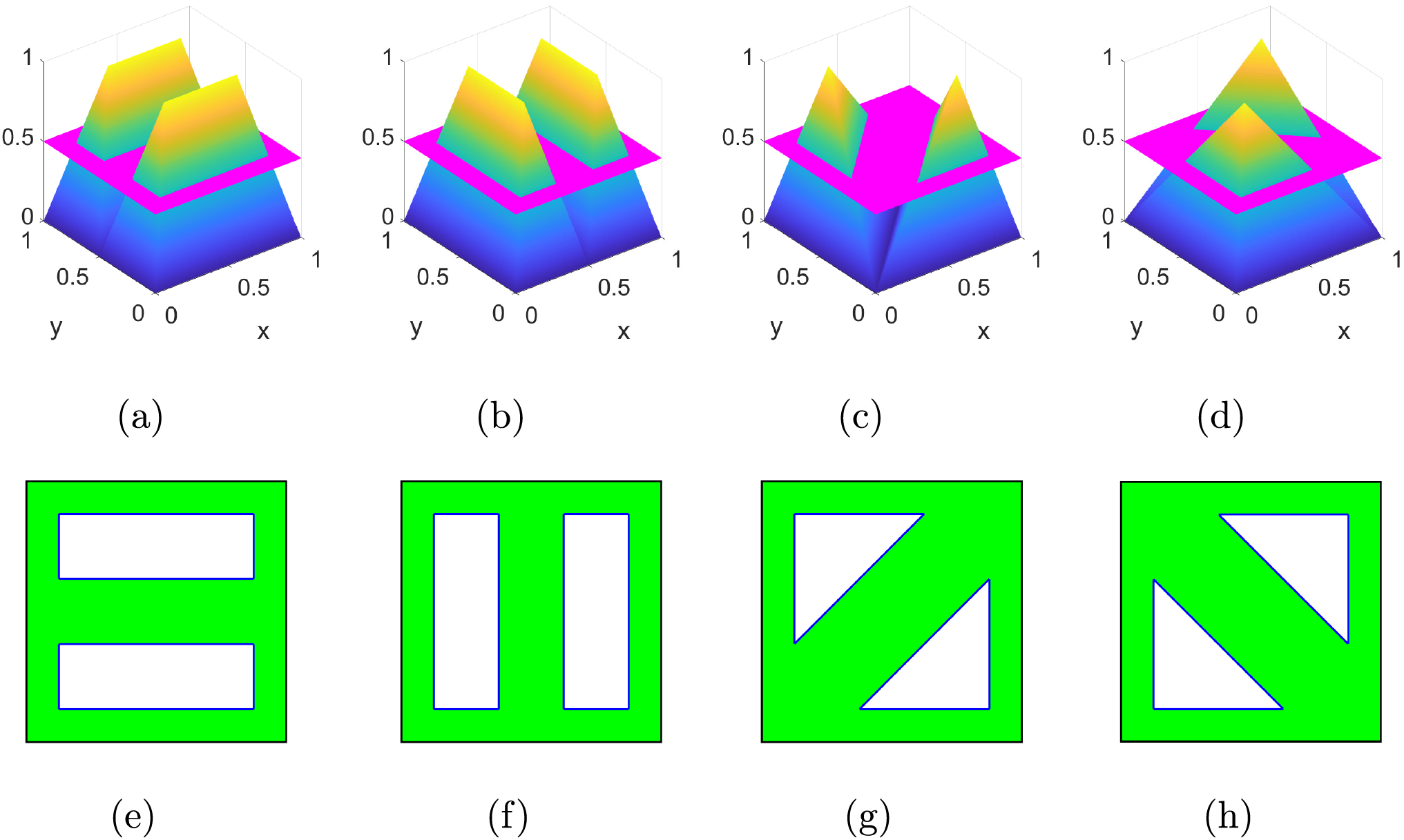
Figure 2: Four basic level set functions and cutting planes (purple horizontal plane), corresponding virtual substructures. (a)–(d) are four basic level set functions and cutting planes with the cutting height of 0.5, while (e)–(h) are the corresponding virtual substructures

The choice of basic level set functions determines the basic configuration of virtual substructures and gives a set of bases that span a space of substructures. In the virtual substructures Ω~i shown in Fig. 2, solid material is distributed in horizontal, vertical, and two diagonal directions, and they offer stiffness in these directions to the actual substructures Ωk obtained by combining Ω~i, i.e.,

Ωk=∪i=1NΩ~i(3)

The combination of virtual substructures Ω~i is implemented by using an intermediate function Υk(x), defined as

Υk(x)=min{Φ1(x)−h1,…,ΦN(x)−hN},x∈Dk,k=1,...,M(4)

Then, Ωk is defined as

Ωk={x|Υk(x)<0,x∈Dk},k=1,...,M(5)

Fig. 3 shows six examples of actual substructures obtained by combining virtual substructures.

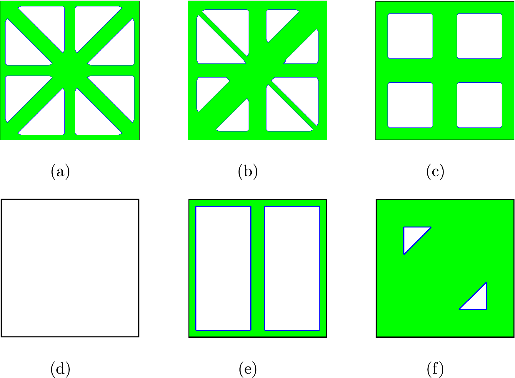
Figure 3: Six examples of actual substructure. (a) h=[0.15,0.15,0.15,0.15]; (b) h=[0.2,0.25,0.25,0.05]; (c) h=[0.35,0.35,0,0]; (d) h=[0,0,0,0]; (e) h=[−0.2,0.2,0,−0.4]; (f) h=[−0.15,0,0.8,−0.25]

2.2 Static Condensation of Substructure

In the finite element analysis, the stiffness matrix of the lattice structure is obtained by assembling the stiffness matrices of substructures, which are obtained by static condensation [20,21].

The concept of static condensation is shown in Fig. 4. Before condensation, the equilibrium equation of a substructure is written as

[KbbKbiKibKii][UbUi]=[FbFi](6)

where the subscript i and b respectively represent internal nodes and boundary nodes; Ub and Ui are respectively the displacement vectors of boundary nodes and internal nodes.

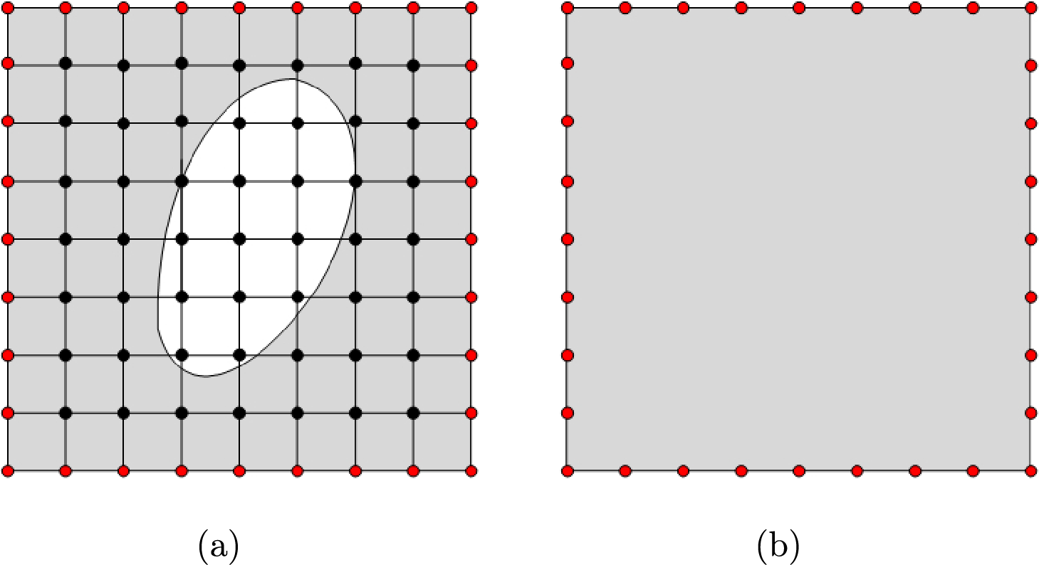
Figure 4: Static condensation of substructure. (a) substructure before static condensation, (b) substructure after static condensation

According to second row of Eq. (6), Ui can be expressed as

Ui=Kii−1[Fi−KibUb](7)

Substitute Eq. (7) into the first row of Eq. (6), the condensed equation can be obtained as

[Kbb−KbiKii−1Kib]Ub=Fb−KbiKii−1Fi(8)

where the coefficient matrix is the condensed stiffness matrix Ksub, i.e.,

Ksub=Kbb−KbiKii−1Kib(9)

Similarly, the force vector of the condensed substructure is given by

Fsub=Fb−KbiKii−1Fi(10)

3  Data-Driven Model of Substructure

The static condensation can reduce the degrees of freedom in the stiffness matrices of substructures, thus improving computational efficiency. However, as the topology optimization progresses, the configurations of substructures will be changed in every iteration; thus, the stiffness matrices need to be condensed again. This process is still time-consuming. In order to avoid repeated static condensation during the optimization, a data-driven model of substructure is proposed in this study.

3.1 Database of Substructures

In order to establish a data-driven model, a database of substructures is first prepared by sampling the space of substructures, i.e., the substructures are obtained by sampling the cutting heights hi (i=1,...,N) in the range of [−0.4,1.4] with a space of 0.2. The admissible range [−0.4, 1.4] is set to ensure the virtual substructures change from full void to full solid. Therefore, there are 104 combinations of cutting heights, which gives 104 samples of substructure. For each sample in this database, the condensed stiffness matrix Ksub and the volume Vsub are computed, and they are stored in the database. With such a database, a numerical mapping model can be constructed to predict the condensed stiffness matrix Ksub and volume Vsub of the substructure based on the cutting heights hi.

3.2 Mapping Model of Substructure

The CS-RBF interpolation is used to construct the mapping model. When an evaluation point is inputted to the mapping model, we search the database for several nearest data points, and the CS-RBF interpolation is used to obtain the condensed stiffness matrix Ksub and volume Vsub of the substructure at the evaluation point.

The evaluation point h is defined as h=[h1,h2,…,hN]T, where N is the number of virtual substructures. The condensed stiffness matrix Ksub and volume Vsub of the substructure are obtained through interpolation functions given by

Kmnsub(h)=∑q=1Qαqmnϕ(rq(h))(11)

Vsub(h)=∑q=1Qγqϕ(rq(h))(12)

where αqmn and γq are the coefficients; Q is the number of data points in the local neighborhood (set to 16 in this study), and ϕ(rq) is the CS-RBF defined as

ϕ(rq)=max{0,(1−rq)4}(4rq+1)(13)

where rq is the function of h and is given by

rq(h)=1ds‖h−h^q‖2+τ2(14)

where h^q are the data points stored in the database, ds is the support radius (set to 2), and τ is a small positive number (set to 0.05) to ensure numerical stability.

The coefficients αqmn and γq are determined by solving a system of equations that enforce the interpolation function to match the data samples in the database. These equations are given by

Kmnsub(h^q)=[K^mnsub]q, q=1,2,...,Q(15)

Vsub(h^q)=V^qsub, q=1,2,...,Q(16)

where K^mnsub and V^sub are respectively the condensed stiffness matrix and volume of substructure stored in the database. The matrix form of Eq. (15) is

[ϕ1,1…ϕ1,Q⋮⋱⋮ϕQ,1…ϕQ,Q][α1mn⋮αQmn]=[[K^mnsub]1⋮[K^mnsub]Q](17)

where ϕi,j is given by

ϕi,j=‖h^i−h^j‖2+τ2,i,j=1,...,Q(18)

Similarly, Eq. (16) can be rewritten in a matrix form.

The accuracy of the CS-RBF interpolation function is verified. Fig. 5 shows the value of K11sub, K14sub, K180sub and Vsub of the substructure when the cutting height h1 is varied from 0 to 1 and h2=0,h3=h4=0.2. The maximum error appears at h1=0.9, where the volume obtained by interpolation is 0.9871 but the truth is 0.9714 (the relative error is 1.62%). From many numerical tests, we see that the CS-RBF interpolation has good accuracy and can be used to construct data-driven models.

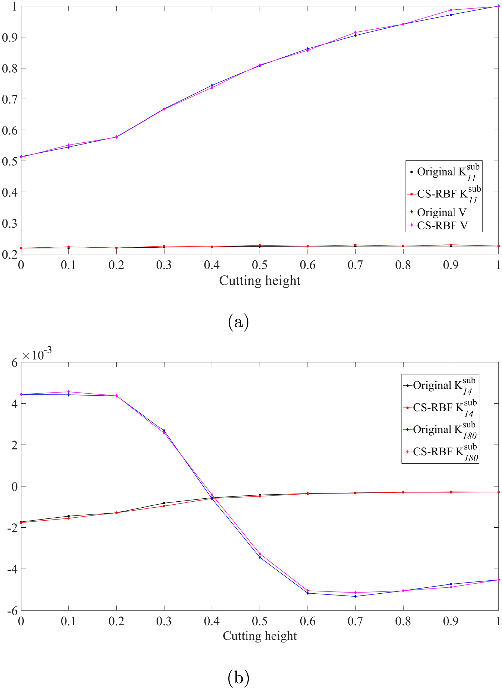
Figure 5: Comparison of interpolation accuracy. (a) is the curve of K11sub and Vsub changing with the first cutting height, and (b) is the curve of K14sub and K180sub changing with the first cutting height

4  Topology Optimization and Sensitivity Analysis of Lattice Structure

The topology optimization problem is defined as

minC=fTu s.t. Ku=fV−V¯≤0h_i≤hik≤h¯i(19)

where C represents the objective function, i.e., the compliance in the present study; f denotes the global force vector; u is the global displacement vector; K stands for the global stiffness matrix; V indicates the volume of the structure, while V¯ is the allowed volume. Additionally, h_i and h¯i define the lower and upper bounds for the height of the cutting planes, respectively. The subscript i is related to the virtual substructure (1≤i≤N), and the superscript k is related to the cell (1≤k≤M).

The design variables of the optimization problem are the cutting heights hi, and the adjoint method is used to compute the sensitivity of design variables. The derivative of C with respect to the cutting height hi is given by

∂C∂hik=−uT∂K∂hiku=−uT∂Ksub,k∂hiku(20)

where Ksub,k is the condensed stiffness matrix of the k-th substructure. According to Eq. (11), we have

∂Kmnsub,k∂hik=∑q=1Qαqmn∂ϕ(rq)∂hik(21)

According to Eq. (13), we have [30]

∂ϕ(rq)∂hik=∂ϕ∂rq∂rq∂hik=max{0,(1−rq)3}(−20rq)∂rq∂hik(22)

where

∂rq∂hik=hik−h^q,ids‖h−h^q‖2+τ2(23)

The derivatives of the volume constraint are also computed. The volume V is obtained from the mapping model, and its sensitivity is calculated similarly to the stiffness matrix.

In the present study, the method of moving asymptote (MMA) is used to solve the optimization problem [31]. Set the move limit parameter to 0.05. The procedure of optimization is shown in Fig. 6. It comprises two stages: the offline stage and the online stage. The purple box represents the construction of the data-driven model of substructure in the offline stage, while the green box represents the online optimization stage.

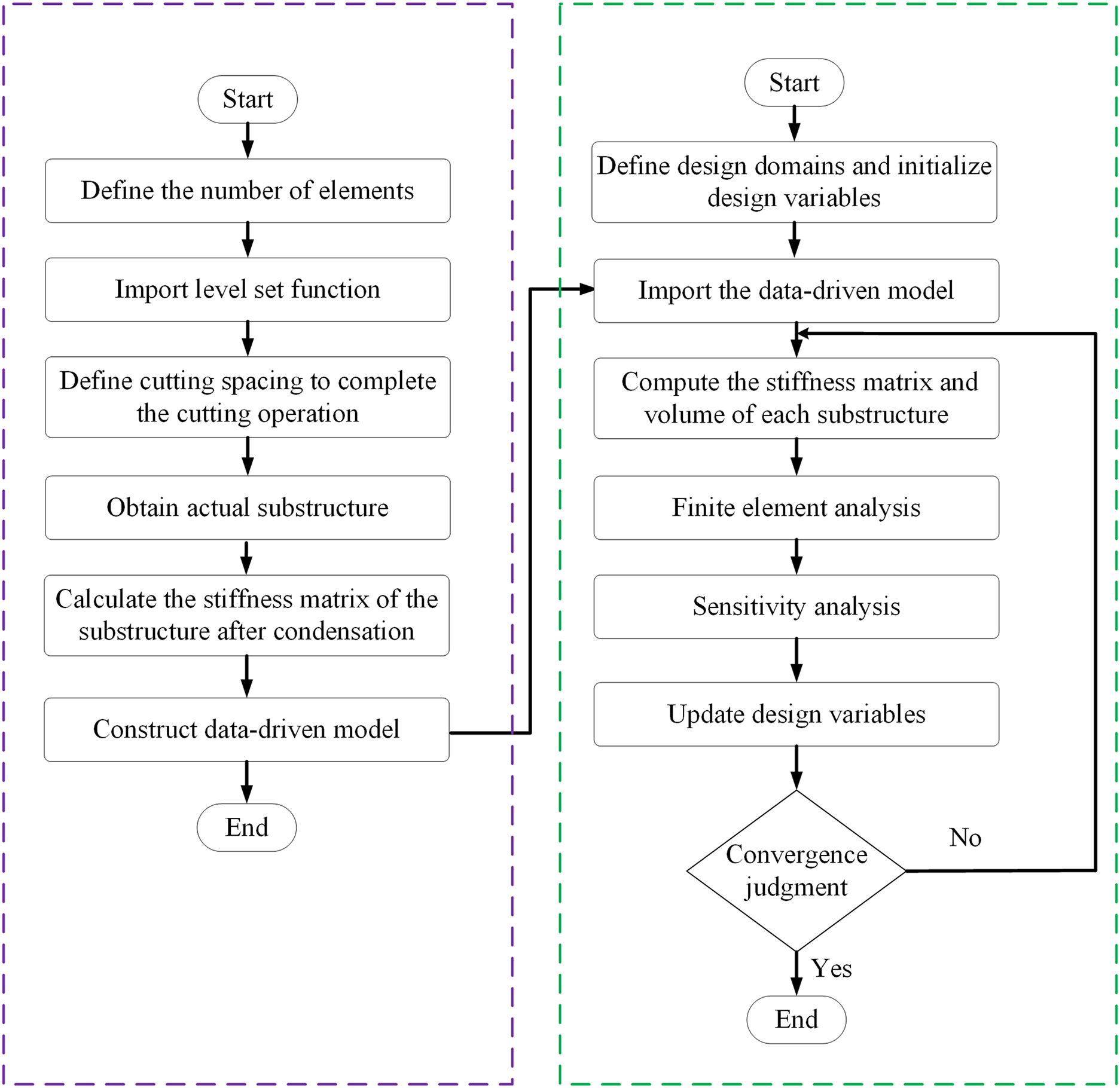
Figure 6: Flowchart of optimization procedure

5  Numerical Example

In this section, several examples of topology optimization were presented. For the topology optimization of two-dimensional lattice structures, Young’s modulus E=1 and Poisson’s ratio of ν=0.3, each substructure is discretized using 40×40 square bilinear elements, and then it is condensed to a super element with 11 points on each edge, and all internal nodes and other nodes in side are condensed. At this time, the degrees of freedom are reduced from 41×41×2=3362 to 10×4×2=80. For a three-dimensional problem, the material parameters are consistent with the two-dimensional problem, substructure is discretized using 20×20×20 elements, and condensed with 11 points on each edge, the size of the condensed stiffness matrix of a substructure is 348×348, while that of the original stiffness matrix is 27,783×27,783. One can see that the size of the stiffness matrix has been significantly reduced. All examples are performed in the same computing environment: Intel Core i9-10900 CPU @ 2.80 GHz. In order to make the optimized structure smoother, a node averaging method was also applied in this study [16,18,32].

The following convergence criteria Eq. (24) is used in all optimizations that include both the method proposed in this paper and the Solid Isotropic Material with Penalization (SIMP) method.

cerr=∑j=15|cs−j+1−cs−5−j+1|∑j=15cs−j+1≤δc(24)

where cerr is the error, s is the current number of iteration, δc is the tolerance of error (set to 0.5%). In addition, the optimization is terminated when the iteration exceeds 150.

5.1 Example 1

The optimization problem of the first example is shown in Fig. 7. The reference design domain is a 5×1 rectangle, with the lower left corner being fixed and the lower right corner being constrained in the vertical direction. A downward force f=1 is applied at the midpoint of the top edge. The allowed volume ratio is 50%. The design domain is discretized into Nx×Ny=100×20 substructures. The initial design is constructed by setting the cutting heights in each substructure to [0.2,0.2,0.25,0.25]T.

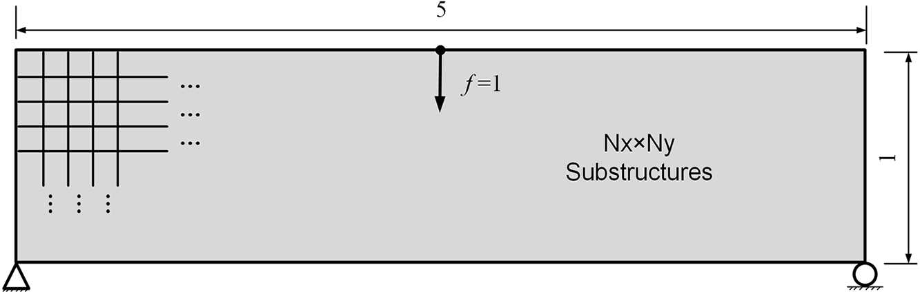
Figure 7: Design problem of the first example

The initial design is shown in Fig. 8a, the compliance is 104.01. The optimized design is shown in Fig. 8b, with a compliance of 79.72. The convergence history is shown in Fig. 8c, it can be seen that the optimization converged smoothly.

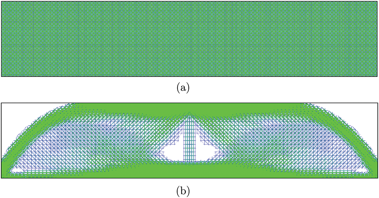
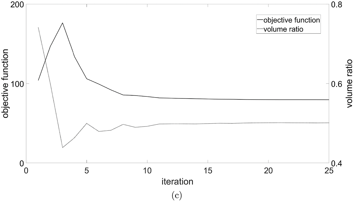
Figure 8: Initial and optimized designs and convergence curve with simply supported beam. Compliance of (a) is 104.01, (b) is 79.72, (c) is the convergence curve

For comparison, a method for directly solving the stiffness matrix of substructures through online condensation has also been considered. As shown in Table 1, it can be found that when directly solving the simply supported beam example online, the finite element calculation time, including calculation of substructure stiffness matrix, is 143.18 s for one iteration, and the final compliance is 83.29. When considering the use of the method proposed in this paper, the finite element calculation time is shortened to 68.28 s, and the compliance is 79.72. Comparison shows that the data-driven approach proposed in this paper can effectively improve the computational efficiency, and the compliance is very close. Besides, a macroscale optimization is also conducted by using the SIMP method [33,34]. Considering that each substructure in this example contains 40×40 elements and there are 100×20 substructures, the finite element mesh is set to 4000×800 in the comparison. Fig. 9 shows the optimized structure obtained by using the SIMP method, and the compliance is 70.33; the compliances of the optimized structures are close.

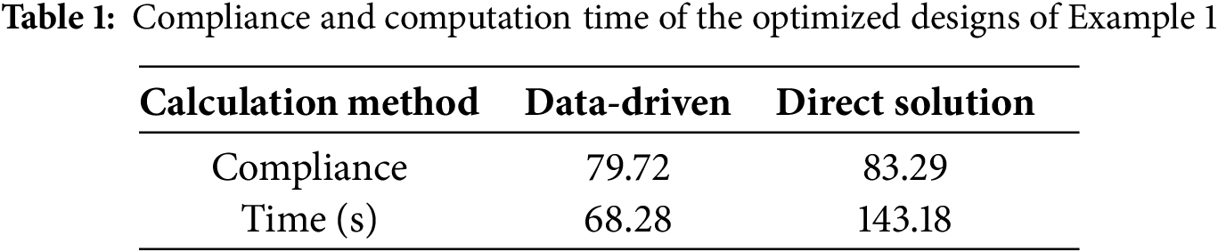
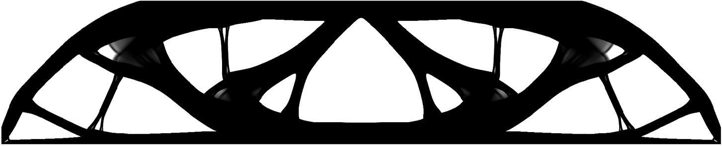
Figure 9: Optimized design by SIMP method with 4000×800 elements, compliance is 70.33

5.2 Example 2

As shown in Fig. 10, the second example has a 2×1 reference design domain. The left side is fixed, and the upper right corner is subjected to a unit concentrated force f=1. The volume fraction is set to 30%.

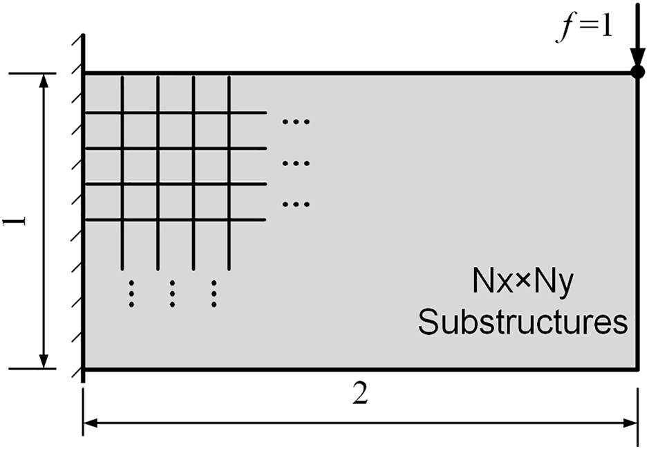
Figure 10: Design problem of the second example

Firstly, the design domain is discretized into Nx×Ny=32×16 substructures. The initial design shown in Fig. 11a is constructed by setting the cutting heights in each substructure to [0.2,0.2,0.25,0.25]T, and its compliance is 116.43. The optimized design is shown in Fig. 11b, with a compliance of 154.82, and the volume is decreased from 74.1% to 30%.

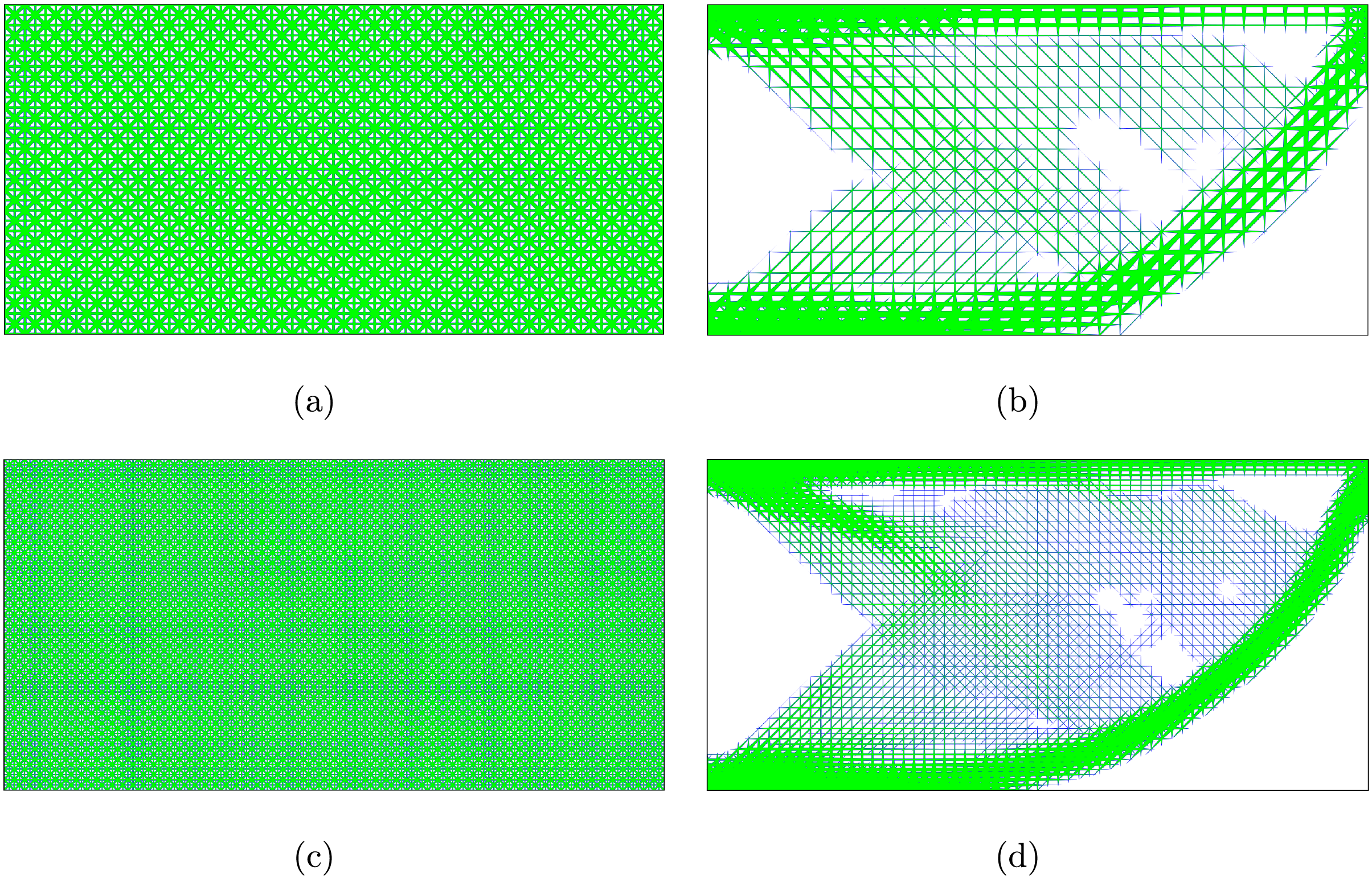
Figure 11: Initial and optimized designs with Nx×Ny=32×16 and Nx×Ny=64×32 substructures. Compliance of (a) is 116.43, (b) is 154.82, (c) is 120.08, (d) is 147.80

Secondly, the optimization is done with the number of substructures being increased to 64×32. The initial design is shown in Fig. 11c, and its compliance is 120.08. The optimized design is shown in Fig. 11d, and its compliance is 147.80. One can see that with more substructures, the compliance of optimized structure is reduced. In addition, comparing Fig. 11b,d, it can be observed that the distribution of substructures is basically consistent.

Similar to Example 1, the method of directly calculating the substructure stiffness matrix online is also considered here. As shown in Table 2, for the same 64×32 substructure problem, the final compliance obtained through direct solution is 153.67, and the calculation time for the finite element part is 144.91 s for one iteration. The compliance by data-driven method is 147.80, and the calculation time for finite element is 71.79 s, which increases the calculation efficiency by more than twice. Also, an optimization at the macro scale is conducted by using the SIMP method [33,34]. Here, the finite element mesh is set to 2560×1280 (corresponding to Fig. 11d with 64×32 substructures). Fig. 12 shows the optimized structure, and the compliance is 134.12. Again, the compliances of the optimized structures are close.

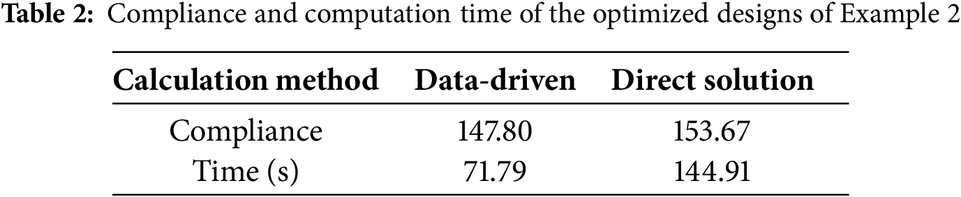
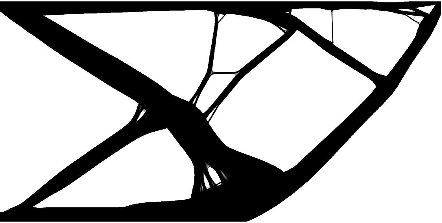
Figure 12: Optimized design by SIMP method with 2560×1280 elements, compliance is 134.12

5.3 Example 3

In the third example, the proposed method is applied to the topology optimization of a thermoelastic lattice structure. The reference design domain is a 2×1 rectangle, with left and right edges being fixed and a force f=1 applied at the midpoint of the bottom, as shown in Fig. 13. The volume fraction of the cantilever beam is set to 20%. The design domain is discretized into Nx×Ny=32×16 substructures. The initial design is constructed by setting the cutting heights in each substructure to [0.2,0.2,0.2,0.2]T. The coefficient of thermal expansion η=0.616. In the FEA of thermoelastic structure, the thermal load vector of the substructure is also obtained by a data-driven model.

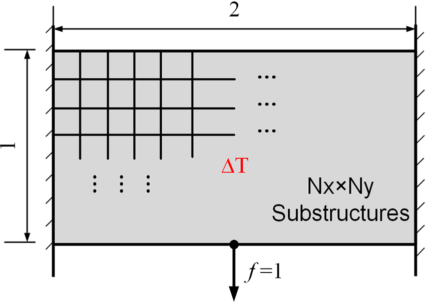
Figure 13: Design problem of the third example

Fig. 14a shows the initial design of the thermoelastic lattice structure. Fig. 14b–d shows the optimized designs at ΔT=5,10,15, respectively, with compliance of 17.83, 28.12, and 36.34. According to Table 3, although the temperature changes, the volume constraint remains at the 20%. Comparing the optimized designs under three different ΔT, it can be seen that temperature is an important factor affecting the optimized configuration of thermoelastic lattice structures.

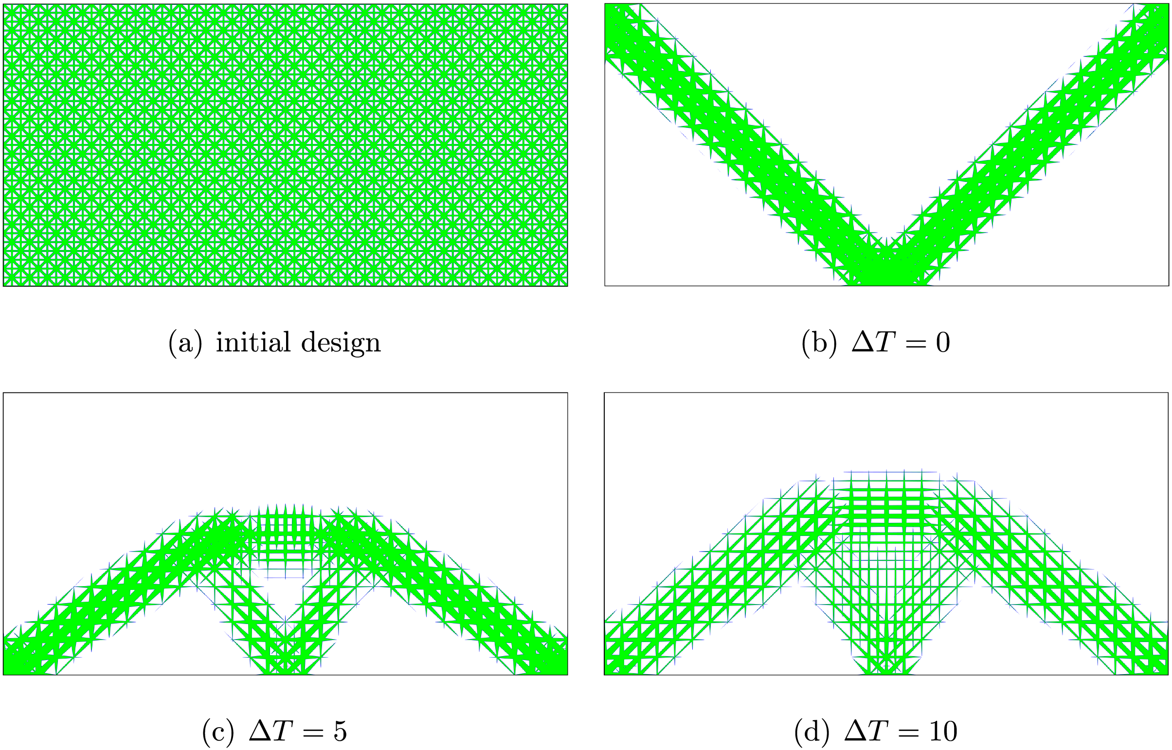
Figure 14: Initial and optimized designs with Nx×Ny=32×16 substructures. Compliance of (a) is 14.50, (b) is 17.83, (c) is 28.12, (d) is 36.34

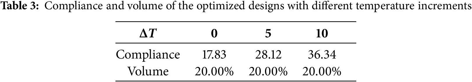
Similarly, the structure is optimized by using the SIMP method with 1280×640 elements and the MMA algorithm (the move limit parameter here is set to 0.05). The optimized structure is shown in Fig. 15, and the compliance is 38.26. As one can see, there are many gray elements in the optimized design, and they implicitly indicate isotropic microstructures. If one needs to determine the configuration of these microstructures, another optimization of the microstructures should be conducted. In comparison, the microstructures are explicitly obtained by the proposed method, as shown in Fig. 14.

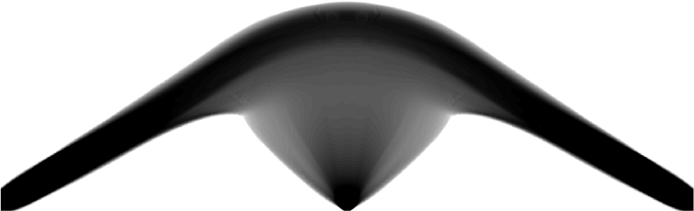
Figure 15: Optimized design by SIMP method with 1280×640 elements, ΔT=10 compliance is 38.26

5.4 Example 4

The fourth example considers a three-dimensional lattice structure, as shown in Fig. 16. The reference design domain is an 8×4×1 cuboid, with the left face fixed and the right bottom edge subjected to uniformly distributed loads q=21N/m. The volume fraction is set to 30%. The design domain is discretized into Nx×Ny×Nz=32×16×4 substructures.

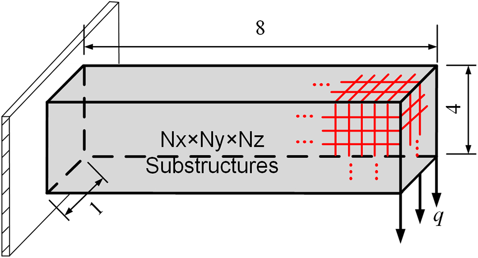
Figure 16: Design problem of the fourth example

Two virtual substructures shown in Fig. 17 are used in the optimization. The initial and optimized designs are shown in Fig. 18, whose compliance is respectively 1544.42 and 2185.53, the volume fraction has decreased from 70.4% to 30%.

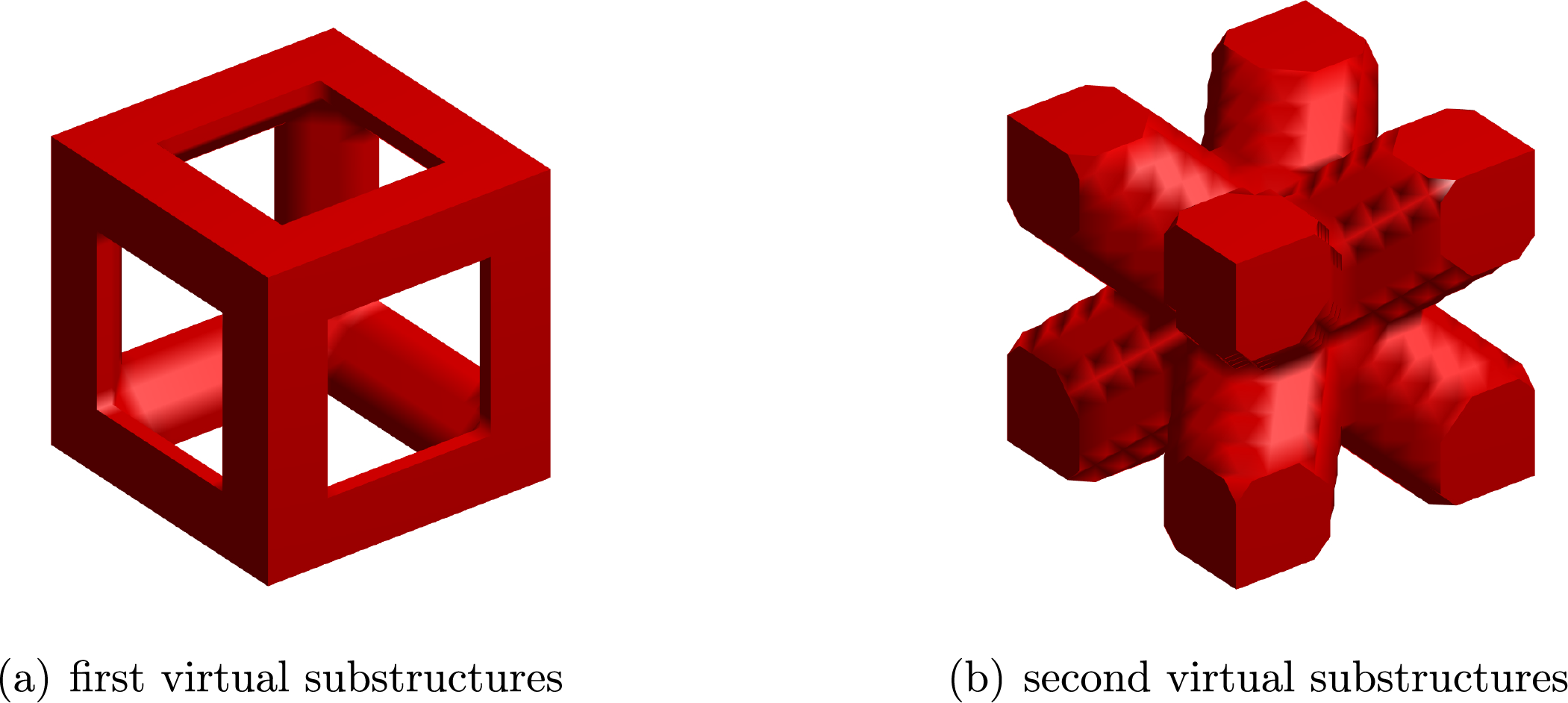
Figure 17: Two 3D virtual substructures. Cutting height (a) h1=0.2, (b) h2=0.2

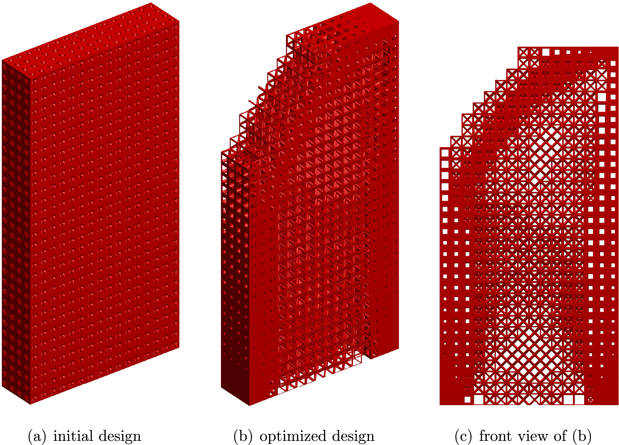
Figure 18: Initial and optimized designs with Nx×Ny×Nz=32×16×4 substructures. Compliance of (a) is 1544.42, (b) is 2185.53, (c) is the front view of the optimized design

6  Conclusion

In this paper, a data-driven model of M-VCUT level set-based substructure is proposed for the topology optimization of lattice structures. The geometries of substructures are described by using the M-VCUT level set method. The condensed stiffness matrix of substructures is obtained by a data-driven model during the optimization, which is computationally efficient, and they are used in the finite element analysis and sensitivity analysis. The data-driven model is constructed by using the CS-RBF interpolation method. The numerical examples demonstrate that the proposed method is effective and efficient for the topology optimization of lattice structures.

In current research, CS-RBF interpolation itself involves computational overhead, especially in solving 3D problems, which is very time-consuming, and the optimization results often contain slim beams that cannot be manufactured. Therefore, in our future work, we will consider multi-scale optimization results that meet manufacturing conditions and more efficient methods.

Acknowledgement: The authors gratefully thank Zhen Liu for providing the code of the substructuring method and Krister Svanberg for providing MMA code support.

Funding Statement: This research work is supported by the National Natural Science Foundation of China (Grant No. 12272144).

Author Contributions: The authors confirm contribution to the paper as follows: study conception and design: Minjie Shao, Qi Xia; data collection: Minjie Shao; analysis and interpretation of results: Minjie Shao, Tielin Shi; draft manuscript preparation: Minjie Shao, Qi Xia, Tielin Shi, Shiyuan Liu. All authors reviewed the results and approved the final version of the manuscript.

Availability of Data and Materials: All data generated or analyzed during this study are included in this published article.

Ethics Approval: Not applicable.

Conflicts of Interest: The authors declare no conflicts of interest to report regarding the present study.

References

1. Wu J, Sigmund O, Groen JP. Topology optimization of multi-scale structures: a review. Struct Multidiscip Optim. 2021;63(3):1455–80. doi:10.1007/s00158-021-02881-8. [Google Scholar] [CrossRef]

2. Wang C, Zhu JH, Wu MQ, Hou J, Zhou H, Meng L, et al. Multi-scale design and optimization for solid-lattice hybrid structures and their application to aerospace vehicle components. Chinese J Aeronaut. 2021;34(5):386–98. doi:10.1016/j.cja.2020.08.015. [Google Scholar] [CrossRef]

3. Aage N, Andreassen E, Lazarov BS, Sigmund O. Giga-voxel computational morphogenesis for structural design. Nature. 2017;550(7674):84–6. doi:10.1038/nature23911. [Google Scholar] [PubMed] [CrossRef]

4. Zhu JH, Zhou H, Wang C, Zhou L, Yuan SQ, Zhang WH. A review of topology optimization for additive manufacturing: status and challenges. Chinese J Aeronaut. 2021;34(1):91–110. doi:10.1016/j.cja.2020.09.020. [Google Scholar] [CrossRef]

5. Mukherjee S, Lu DC, Raghavan B, Breitkopf P, Dutta S, Xiao MY, et al. Accelerating large-scale topology optimization: state-of-the-art and challenges. Arch Computat Methods Eng. 2021;28(7):1–23. doi:10.1007/s11831-021-09544-3. [Google Scholar] [CrossRef]

6. Bendsoe MP, Kikuchi N. Generating optimal topologies in structural design using a homogenization method. Comput Methods Appl Mech Eng. 1988;71(2):197–224. doi:10.1016/0045-7825(88)90086-2. [Google Scholar] [CrossRef]

7. Dong GY, Tang YL, Zhao YYF. A 149 line homogenization code for three-dimensional cellular materials written in matlab. J Eng Mater-T ASME. 2019;141(1):011005. doi:10.1115/1.4040555. [Google Scholar] [CrossRef]

8. Groen JP, Sigmund O. Homogenization-based topology optimization for high-resolution manufacturable microstructures. Int J Numer Methods Eng. 2018;113(8):1148–63. doi:10.1002/nme.5575. [Google Scholar] [CrossRef]

9. Allaire G, Geoffroy-Donders P, Pantz O. Topology optimization of modulated and oriented periodic microstructures by the homogenization method. Comput Math Appl. 2019;78(7):2197–229. doi:10.1016/j.camwa.2018.08.007. [Google Scholar] [CrossRef]

10. Wang YJ, Xu H, Pasini D. Multiscale isogeometric topology optimization for lattice materials. Comput Methods Appl Mech Eng. 2017;316:568–85. doi:10.1016/j.cma.2016.08.015. [Google Scholar] [CrossRef]

11. Chen WJ, Tong LY, Liu ST. Concurrent topology design of structure and material using a two-scale topology optimization. Comput Struct. 2017;178:119–28. doi:10.1016/j.compstruc.2016.10.013. [Google Scholar] [CrossRef]

12. Wang YG, Kang Z. Concurrent two-scale topological design of multiple unit cells and structure using combined velocity field level set and density model. Comput Methods Appl Mech Eng. 2019;347:340–64. doi:10.1016/j.cma.2018.12.018. [Google Scholar] [CrossRef]

13. Wang YJ, Li XQ, Long K, Wei P. Open-source codes of topology optimization: a summary for beginners to start their research. Comp Model Eng. 2023;137(1):1–34. doi:10.32604/cmes.2023.027603. [Google Scholar] [CrossRef]

14. Wei GK, Chen Y, Li Q, Fu KK. Multiscale topology optimisation for porous composite structures with stress-constraint and clustered microstructures. Comput Methods Appl Mech Eng. 2023;416:116329. doi:10.1016/j.cma.2023.116329. [Google Scholar] [CrossRef]

15. Cheng L, Bai JX, To AC. Functionally graded lattice structure topology optimization for the design of additive manufactured components with stress constraints. Comput Methods Appl Mech Eng. 2019;344(5):334–59. doi:10.1016/j.cma.2018.10.010. [Google Scholar] [CrossRef]

16. Wang YJ, Arabnejad S, Tanzer M, Pasini D. Hip implant optimization design with three-dimensional porous material of graded density. AMSE J Mech Des. 2018;140(11):111406. doi:10.1115/1.4041208. [Google Scholar] [CrossRef]

17. Chen XL, Liu H, Wei P. Extended multiscale fem-based concurrent optimization of three-dimensional graded lattice structures with multiple microstructure configurations. Compos Struct. 2024;341:118186. doi:10.1016/j.compstruct.2024.118186. [Google Scholar] [CrossRef]

18. Wu TY, Li S. An efficient multiscale optimization method for conformal lattice materials. Struct Multidiscip O. 2021;63(3):1063–83. doi:10.1007/s00158-020-02739-5. [Google Scholar] [CrossRef]

19. Huang MC, Du ZL, Liu C, Zheng YG, Cui TC, Mei Y, et al. Problem-independent machine learning (piml)-based topology optimization-a universal approach. Extreme Mech Lett. 2022;56:101887. doi:10.1016/j.eml.2022.101887. [Google Scholar] [CrossRef]

20. Wu ZJ, Xia L, Wang ST, Shi TL. Topology optimization of hierarchical lattice structures with substructuring. Comput Methods Appl Mech Eng. 2019;345(2):602–17. doi:10.1016/j.cma.2018.11.003. [Google Scholar] [CrossRef]

21. Liu Z, Xia L, Xia Q, Shi TL. Data-driven design approach to hierarchical hybrid structures with multiple lattice configurations. Struct Multidiscip Optim. 2020;61(6):2227–35. doi:10.1007/s00158-020-02497-4. [Google Scholar] [CrossRef]

22. Huang MC, Liu C, Guo YL, Zhang LF, Du ZL, Guo X. A mechanics-based data-free problem independent machine learning (piml) model for large-scale structural analysis and design optimization. J Mech Phys Solids. 2024;193(7674):105893. doi:10.1016/j.jmps.2024.105893. [Google Scholar] [CrossRef]

23. Wu ZJ, Fan F, Xiao RB, Yu LQ. The substructuring-based topology optimization for maximizing the first eigenvalue of hierarchical lattice structure. Int J Numer Meth Eng. 2020;121(13):2964–78. doi:10.1002/nme.6342. [Google Scholar] [CrossRef]

24. Fu JJ, Xia L, Gao L, Xiao M, Li H. Topology optimization of periodic structures with substructuring. J Mech Design. 2019;141(7):071403. doi:10.1115/1.4042616. [Google Scholar] [CrossRef]

25. Liu H, Zong HM, Shi TL, Xia Q. M-VCUT level set method for optimizing cellular structures. Comput Methods Appl Mech Eng. 2020;367(8):113154. doi:10.1016/j.cma.2020.113154. [Google Scholar] [CrossRef]

26. Xia Q, Zong HM, Shi TL, Liu H. Optimizing cellular structures through the m-vcut level set method with microstructure mapping and high order cutting. Compos Struct. 2021;261(3):113298. doi:10.1016/j.compstruct.2020.113298. [Google Scholar] [CrossRef]

27. Zhou J, Shao MJ, Tian Y, Xia Q. Concurrent two-scale topology optimization of thermoelastic structures using a m-vcut level set based model of microstructures. Comp Model Eng. 2024;141(2):1327–45. doi:10.32604/cmes.2024.054059. [Google Scholar] [CrossRef]

28. Buhmann MD. Radial basis functions: theory and implementations. In: Cambridge monographs on applied and computational mathematics. Vol. 12. New York, NY, USA: Cambridge University Press; 2004. [Google Scholar]

29. Wang SY, Wang MY. Radial basis functions and level set method for structural topology optimization. Int J Numer Meth Eng. 2006;65(12):2060–90. doi:10.1002/nme.1536. [Google Scholar] [CrossRef]

30. Wei P, Li Z, Li X, Wang MY. An 88-line Matlab code for the parameterized level set method based topology optimization using radial basis functions. Struct Multidiscip Optim. 2018;58(2):831–49. doi:10.1007/s00158-018-1904-8. [Google Scholar] [CrossRef]

31. Svanberg K. The method of moving asymptotes-a new method for structural optimization. Int J Numer Methods Eng. 1987;24(2):359–73. doi:10.1002/nme.1620240207. [Google Scholar] [CrossRef]

32. Liu H, Chen LX, Bian H. Data-driven m-vcut topology optimization method for heat conduction problem of cellular structure with multiple microstructure prototypes. Int J Heat Mass Tran. 2022;198(7646):123421. doi:10.1016/j.ijheatmasstransfer.2022.123421. [Google Scholar] [CrossRef]

33. Andreassen E, Clausen A, Schevenels M, Lazarov BS, Sigmund O. Efficient topology optimization in matlab using 88 lines of code. Struct Multidiscip O. 2011;43(1):1–16. doi:10.1007/s00158-010-0594-7. [Google Scholar] [CrossRef]

34. Sigmund O. A 99 line topology optimization code written in matlab. Struct Multidiscip O. 2001;21(2):120–7. doi:10.1007/s001580050176. [Google Scholar] [CrossRef]