
 Submit a Paper
 Propose a Special lssue
 Open Access
ARTICLE

Investigating the Role of Antimalarial Treatment and Mosquito Nets in Malaria Transmission and Control through Mathematical Modeling
1 Department of Mathematics and Statistics, College of Science, King Faisal University, Al-Ahsa, 31982, Saudi Arabia
2 Department of Mathematics, Government College University, Lahore, 54000, Pakistan
3 Tandy School of Computer Science, University of Tulsa, Tulsa, OK 74104, USA
4 School of Finance and Operations Management, University of Tulsa, Tulsa, OK 74104, USA
5 Polytechnic Institute, University of Oklahoma, Tulsa, OK 74135, USA
* Corresponding Authors: Azhar Iqbal Kashif Butt. Email: ; Tariq Ismaeel. Email:
(This article belongs to the Special Issue: Advances in Mathematical Modeling: Numerical Approaches and Simulation for Computational Biology)
Computer Modeling in Engineering & Sciences 2025, 144(3), 3463-3492. https://doi.org/10.32604/cmes.2025.069277
Received 19 June 2025; Accepted 20 August 2025; Issue published 30 September 2025
 View Full Text
 Download PDF
Abstract
Malaria is a significant global health challenge. This devastating disease continues to affect millions, especially in tropical regions. It is caused by Plasmodium parasites transmitted by female Anopheles mosquitoes. This study introduces a nonlinear mathematical model for examining the transmission dynamics of malaria, incorporating both human and mosquito populations. We aim to identify the key factors driving the endemic spread of malaria, determine feasible solutions, and provide insights that lead to the development of effective prevention and management strategies. We derive the basic reproductive number employing the next-generation matrix approach and identify the disease-free and endemic equilibrium points. Stability analyses indicate that the disease-free equilibrium is locally and globally stable when the reproductive number is below one, whereas an endemic equilibrium persists when this threshold is exceeded. Sensitivity analysis identifies the most influential mosquito-related parameters, particularly the bite rate and mosquito mortality, in controlling the spread of malaria. Furthermore, we extend our model to include a treatment compartment and three disease-preventive control variables such as antimalaria drug treatments, use of larvicides, and the use of insecticide-treated mosquito nets for optimal control analysis. The results show that optimal use of mosquito nets, use of larvicides for mosquito population control, and treatment can lower the basic reproduction number and control malaria transmission with minimal intervention costs. The analysis of disease control strategies and findings offers valuable information for policymakers in designing cost-effective strategies to combat malaria.Keywords
Malaria is a contagious disease caused by Plasmodium parasites, mainly transmitted to humans through the bite of a female mosquito [1]. Although there has been significant progress in decreasing the number of malaria cases worldwide, the disease continues to pose an important public health challenge, especially in tropical and subtropical regions. The groups at risk include children under the age of five, pregnant women, and travelers who lack immunity [1,2]. Travelers from countries without local malaria transmission are at significant risk of contracting malaria and its consequences when traveling abroad, as they lack immunity. Additionally, individuals who leave malaria-endemic countries and immigrate to malaria-free nations are also at risk when they return to their home countries to visit friends and family, as their immunity wanes or becomes nonexistent. However, Sub-Saharan Africa remains the most vulnerable region, representing a significantly high share of deaths attributed to malaria [3].
Female mosquitoes that transmit disease have salivary glands that contain sporozoites. In the human body, these sporozoites develop into two forms: erythrocytic and hepatocyte schizogony. During the hepatocyte phase, the sporozoite transforms into a hypnozoite, a dormant form, which later develops into a schizont [4]. The schizont undergoes rapid cell division, producing merozoites that infect red blood cells. Meanwhile, hypnozoites can remain dormant for an extended period. The merozoites produced in the liver invade red blood cells, thereby sustaining the cycle of infection [5]. Trophozoites form and associate with merozoites, developing into blood schizonts that produce merozoites to infect new red blood cells. In some plasmodium parasites, hypnozoites develop into liver schizonts that burst, releasing a large number of merozoites after 8 to 10 months. The number of sporozoites injected by mosquitoes into humans is a crucial factor in the recurrence of malaria [6].
To mitigate the impact of malaria on the global population, various scientific initiatives have been undertaken, including the development of mathematical models [7,8]. The SEIR model, introduced by Kermack and McKendrick, has been widely adopted for modeling malaria transmission [9–11]. Since then, numerous mathematical models have been developed to combat malaria and reduce its global mortality rate [12–14]. However, predicting the severity of malaria remains a challenging task despite these efforts. As climate change awareness grows, it’s essential to recognize the significant impact of climatic and environmental conditions on the spread and transmission of vector-borne diseases [15]. Environmental factors like temperature, rainfall, humidity, wind speed, and daylight duration play a crucial role in shaping the seasonal and daily rhythms of mosquito populations, influencing their ecological and behavioral aspects [16].
Mathematical modeling has become a powerful tool in understanding the transmission dynamics of malaria [17–21]. In [22], the primary focus was on the development of a mathematical model and the evaluation of two disease control strategies: human precautions and mosquito sprays. The study determined that the system achieves a disease-free state when at least 40% of susceptible humans undertake the necessary precautions. In another study [23], the authors proposed an effective disease control approach known as awareness-based intervention, which utilizes media for malaria management. The model incorporates time-dependent control measures for treatment, insecticides, and social media initiatives to minimize the costs associated with malaria control. A new mathematical model using partial differential equations was developed for malaria in [24]. The authors studied the effectiveness of spraying in malaria control and found that uniform spraying produced comparable results to a non-spatial model.
Most mathematical models overlook the mosquito life cycle, excluding eggs, larvae, and pupae from the transmission cycle. While this simplification is helpful, it leads to a significant limitation: these models often struggle to accurately predict the magnitude of malaria in regions where it is most prevalent. To comprehensively understand the complex processes driving malaria transmission and develop more accurate predictive models, it is essential to consider the mosquito life cycle and the impacts of seasonality [25]. Moulay et al. [26] recently developed a mathematical model that simulates the dynamics of mosquito populations, incorporating the self-regulatory mechanisms of the egg and larval stages. They identified a threshold that plays a crucial role in controlling mosquito population growth. However, these models often overlook important factors like the life cycle of mosquitoes and variations in the environment. This can lead to inaccuracies in predicting the severity of the disease, particularly in areas where malaria is widespread.
In comparison to earlier models [22–26] that either assume a constant mosquito population or neglect the impact of treatments, this study addresses these shortcomings by integrating the dynamics of mosquito populations and seasonal variations into a non-linear mathematical model. It also presents a more comprehensive model that incorporates both symptomatic and asymptomatic human infections, considers the different stages of the mosquito life cycle, and integrates treatment effects with vector control. This approach improves realism and facilitates the examination of integrated control strategies. Overall, the combination of stability analysis, detailed compartmental dynamics, and optimal control within realistic constraints represents a significant advancement that differentiates it from existing approaches in both scope and suitability. We will explore the most efficient approaches to managing the disease, emphasizing the utilization of anti-malaria medications, vector control methods to reduce mosquito populations, and the use of mosquito nets.
The sections of the article are arranged as follows. Section 2 outlines the formulation of the model, which divides human and mosquito populations into different compartments and uses a set of nonlinear ordinary differential equations (ODEs) to represent the spread of the disease. In Section 3, we present theoretical findings, including the existence, uniqueness, positivity, and boundedness of the model’s solutions. The stability analysis of disease-free equilibrium (DFE), and endemic equilibrium (EE) with respect to reproduction number
2 Mathematical Modeling of Malaria
We develop an extended SEIR-based mathematical model that incorporates asymptomatic human cases and vector populations, capturing the complex dynamics of malaria transmission more effectively than classical models. The SEIR type models are particularly effective for modeling malaria because they include a latency period in both human and mosquito populations. The model will analyze how human and mosquito populations change over time, with humans represented as
The infection period of mosquitoes is directly correlated with their relatively short life. Therefore, our model focuses exclusively on mature mosquitoes, as their maturity aligns with their infection period. At any given time
and
The growth rate of mosquitoes is represented by
and hence the susceptible mosquitoes move to the exposed class at this rate. The exposed mosquitoes become infectious at the rate
The susceptible humans are recruited at a constant birth rate
The humans exposed to the virus become infectious, which can further be divided into two subgroups: symptomatic and asymptomatic. The rate at which symptomatic individuals develop symptoms is denoted by
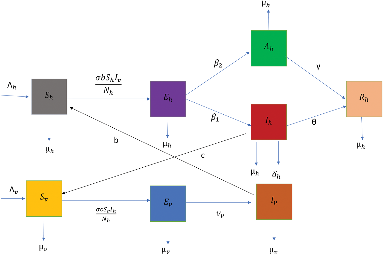
Figure 1: Diagram showing the transmission of disease through the compartments
The malaria parasite transmission flow diagram is transformed into the following system of nonlinear ODEs:
with initial conditions that are non-negative, i.e.,
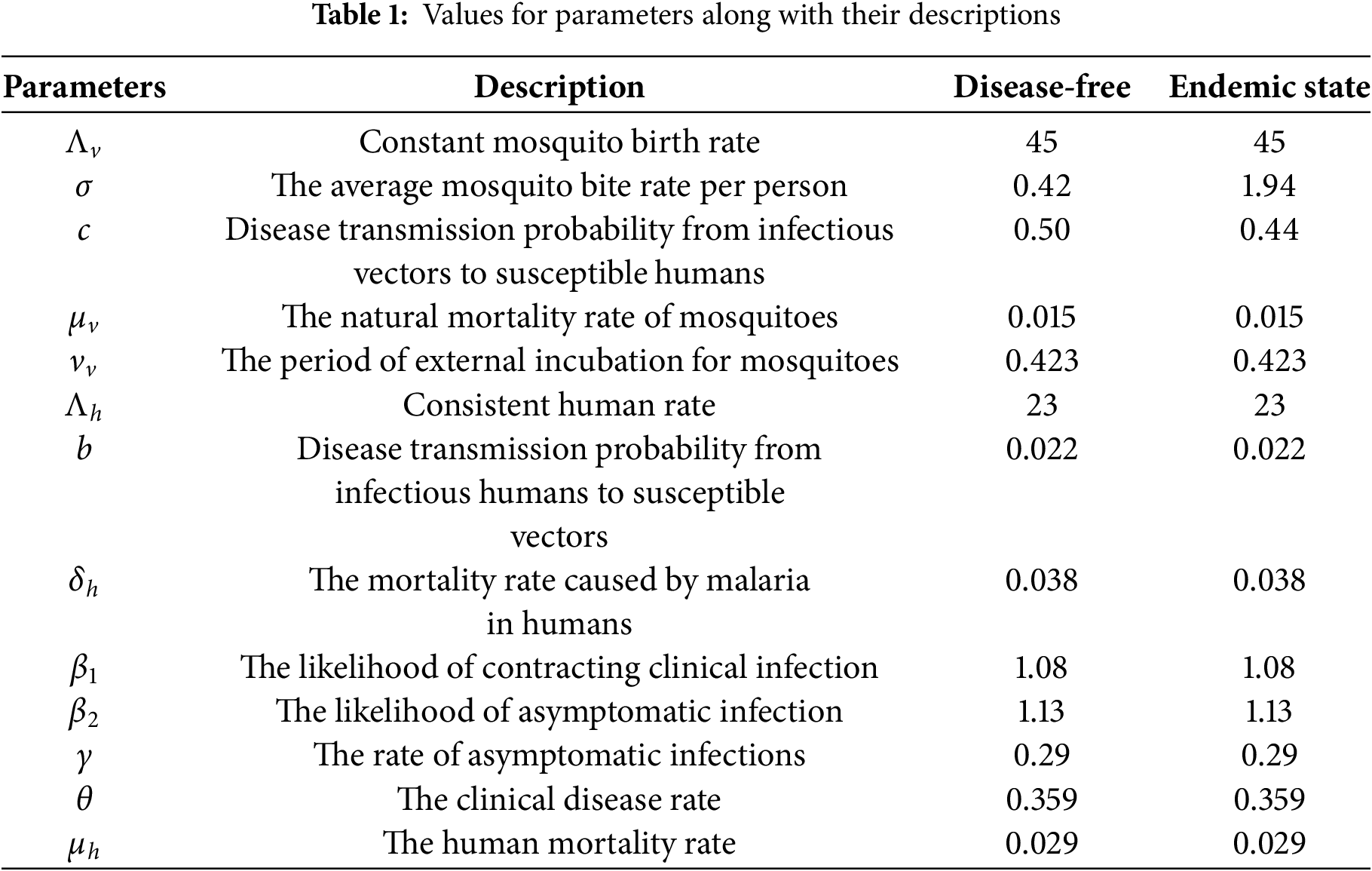
Table 1 presents the model parameters’ descriptions and values. In compact form, we put the model (3) as follows:
where
with
and
In this section, we present the main theoretical results, demonstrating the physical viability of the proposed mathematical model and its potential for further exploration in numerical simulations. We establish the uniqueness of the solution of the model (3) and verify that the solution of each state equation remains positive and bounded for all
3.1 Positivity and Boundedness of the Solutions
We aim to establish that the variable
Theorem 1: The solution
Proof: The Eq. (3f) can be rewritten as:
or
where
The differential Eq. (6) yields us an integrated factor
Integrating the above equation over the interval
After simplification, we obtain the following expression for
Given
Theorem 2: The solution
Proof: Differentiating Eqs. (1) and (2) with respect to time
and
with
and
Suppose for any given initial condition, if
then
Similarly if
then
We employ the Grönwall’s inequality to determine the following solutions.
and
This implies that
and
Thus, we can write the following inequalities.
which proves the boundedness of
As a result of the above two theorems, the feasible region for the proposed model (3) is defined as follows.
To demonstrate the existence and uniqueness of the solutions of the disease model (3), we present the following foundational results of [27,28].
Theorem 3: Consider the domain
where
Theorem 4: If
then for
We now introduce the theorem that establishes the existence of a unique solution for IVP (4).
Theorem 5: Assume that the domain for the problem (4) is
Proof: Here, the function
All other first-order derivatives are equal to zero, i.e.,
Here
Thus,
This proves the existence of a unique solution of the disease model (4). □
We determine the Disease-Free Equilibrium (DFE) point by setting
The endemic equilibrium point represents a stable state in which the disease continues to persist and circulate within the population with a constant number of infected individuals who coexist within the population. In this scenario, the disease persists in both the mosquito and human populations, which means
where
and
The reproduction number
To determine
The jacobian matrices F and V are then determined as follows:
where
Thus,
The reproduction number,
3.5 Stability Characterization of Model
This section investigates the stability of the malaria mathematical model, analyzing both local and global stability at the equilibrium points of DFE and EE.
3.5.1 Evaluation of Local Stability
To evaluate the local stability of the model at the DFE point, the Jacobian matrix is calculated and evaluated at
We introduce the following theorem to analyze the local stability of model (3) at the DFE point
Theorem 6: State model (3) is locally asymptotically stable at
Proof: The Jacobian matrix (15) has the following eigenvalues.
The eigenvalues (
3.5.2 Evaluation of Global Stability
This section presents a global stability analysis of the model, focusing on the disease-free equilibrium and the epidemic equilibrium points. We employed the Castillo-Chavez approach to investigate global stability at the DFE point (
To establish global stability at the DFE point (
Here,
Here,
Lemma 1: If conditions
Now, we proceed to confirm the following theorem.
Theorem 7: The DFE point,
Proof: We define
If
As
Now,
where,
The matrix
The following theorem illustrates the global stability of model (3) at the endemic equilibrium point
Theorem 8: For disease model (3), if
Proof: A Volterra-type Lyapunov function is a powerful tool for establishing global stability. The function is defined as:
The equilibrium point
or
We substitute the derivatives in the equation with the right-hand side of the ODEs of the model (3), resulting in the following expression.
After rearranging the terms on the right-hand side, we obtain:
The above derivative expression for L can be rearranged to take the following form.
where
and
Thus,
Global stability means that the system converges to the endemic equilibrium point
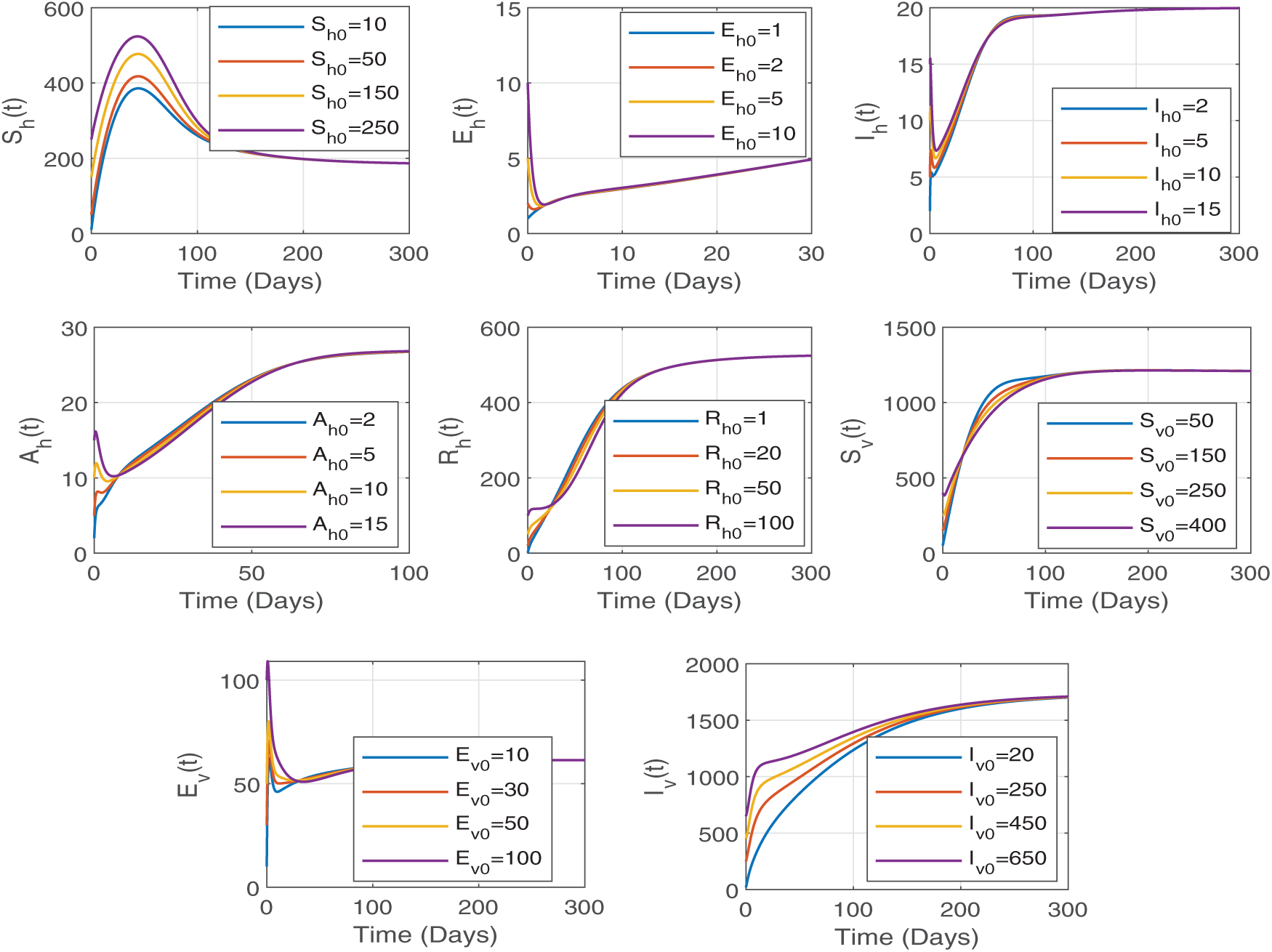
Figure 2: Figure displays the numerical evidence of global stability where the system trajectories converge to the endemic equilibrium point for any positive initial conditions
Sensitivity analysis is crucial in formulating successful strategies to restrict or reduce the effect of a pandemic. Using sensitivity analysis tools, we can identify the parameters with the highest sensitivity to
The sensitivity of a parameter of the reproduction number
that gives the sensitivity index of the parameter
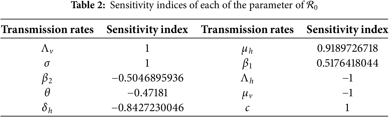
The sensitivity indices in the given table provide valuable information about how modifications to certain parameters impact the reproduction number
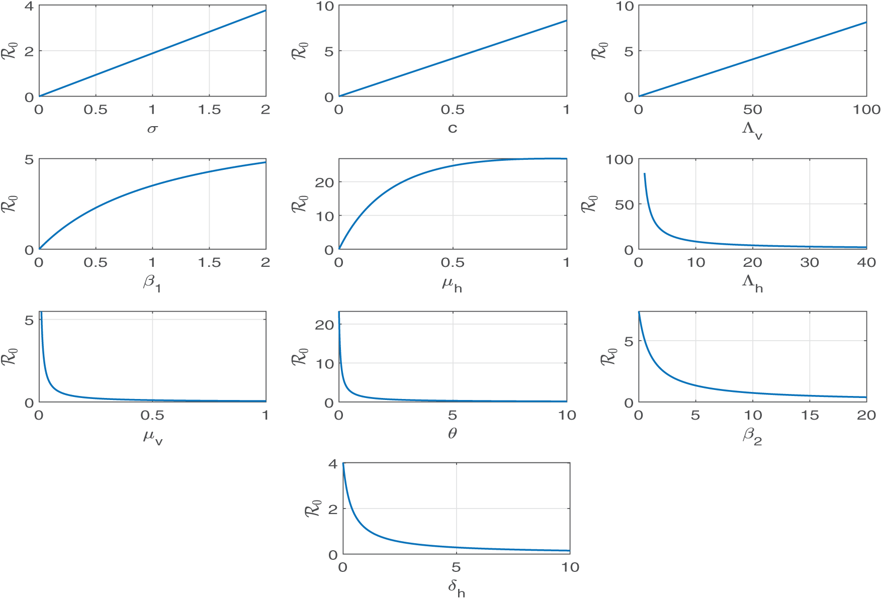
Figure 3: The parameters
Therefore, implementing specific control strategies aimed at decreasing transmission rates
5 Malaria Model for Disease Control
In this section, we extend the model outlined in (3) by adding a treat compartment T and adjusting three time-dependent control variables
The revised system of ordinary differential equations with controls is presented as follows.
with initial conditions:
where
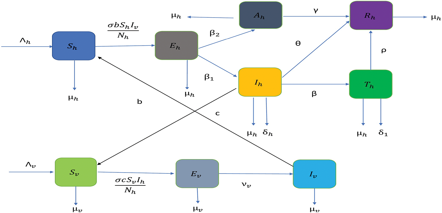
Figure 4: Flow diagram of an updated malaria model where we have incorporated a treatment compartment as a disease control strategy
5.1 Positive and Bounded Solutions
To demonstrate that the solutions of the malaria model (22) are positive and bounded for all
Theorem 9: The solution
Theorem 10: The solution
The proof of these two theorems is similar to the proof of Theorems 1 and 2 presented for model (3).
5.2 Disease-Free Equilibrium Point and Reproduction Number
We solve the steady-state equations of the extended disease model (22) by considering
To derive the reproduction number for the modified malaria model (22), we divide the population into infected and uninfected compartments. The infected compartment includes individuals exposed to mosquitoes, infected mosquitoes, exposed humans, and those who are clinically and asymptomatically infected and have received treatment. All others are considered uninfected.
To determine
where
The spectral radius of the malaria transmission model is given by the maximum absolute value among the eigenvalues of
The dynamics of the state variables, as shown in Fig. 5, illustrate two key scenarios based on the basic reproduction number,
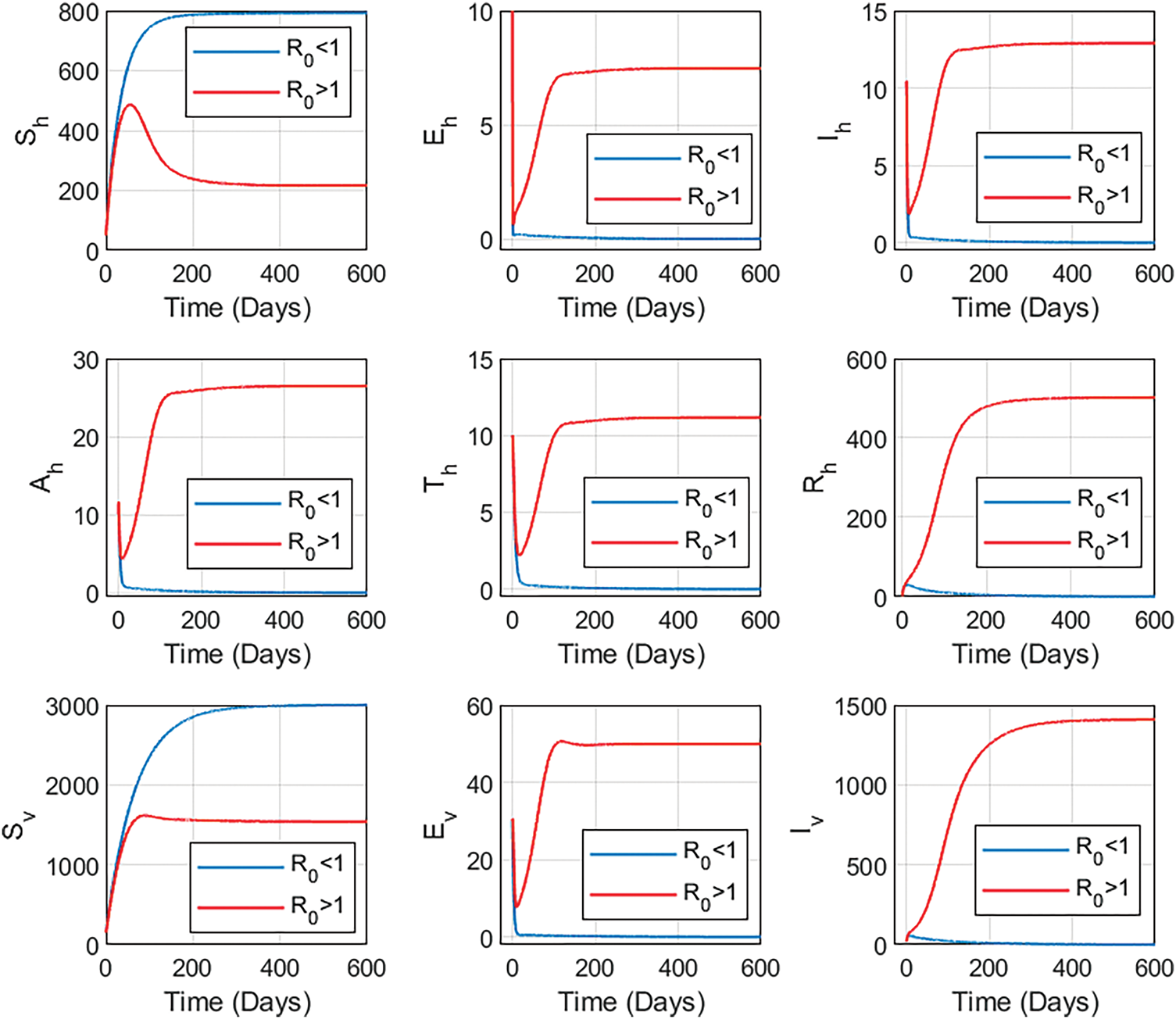
Figure 5: Figure illustrates two key scenarios based on the basic reproduction number,
This section presents the most effective strategies to minimize the population’s exposure to disease. It aims to prevent malaria through the use of mosquito nets, insecticides, and anti-malaria medications. By formulating an optimal control problem, we determine the optimal conditions necessary to achieve this goal [32–36].
We consider the following cost functional to formulate an optimal control problem to implement disease control strategies.
In this context,
The objective is to minimize the cost functional (23), leading to determine the optimal control
To derive the prerequisites for an effective control problem, Pontryagin’s Maximum Principle is employed. The condition is expressed in terms of the Hamiltonian,
where
The first optimality condition is met when
which leads us to the following expressions for the control variables.
We impose bounds on control variables to ensure that the model remains realistic and feasible.
The second optimality condition:
results in an adjoint system of linear ordinary differential equations:
supported with the following terminal conditions:
The derivative of
Algorithm 1 outlines the procedure employed to derive an optimal solution
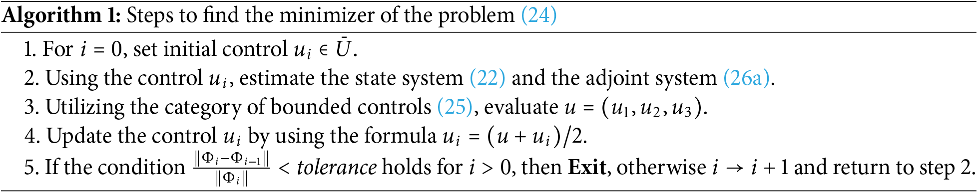
With
6.3 Optimal Solutions and Discussions
In this section, we present a comprehensive analysis of the solutions to the optimal control problem outlined in Algorithm 1. The optimal solutions are obtained using the proposed algorithm along with its implementation in MATLAB. To discretize the state Eq. (22) and the adjoint Eq. (26a), we implement the Fourth-order Runge-Kutta (RK4) method. The continuous time domain
In this analysis, three control variables are examined, and their impact on both the mosquito and human populations is illustrated through graphical representations. These visualizations highlight the influence of controls on disease dynamics and offer valuable insight into the effectiveness of the strategies implemented.
The profiles of the optimized control variables are illustrated in Fig. 6. It can be seen that all three controls begin at relatively high levels and then gradually decrease over time (days). At the beginning, a strong implementation of
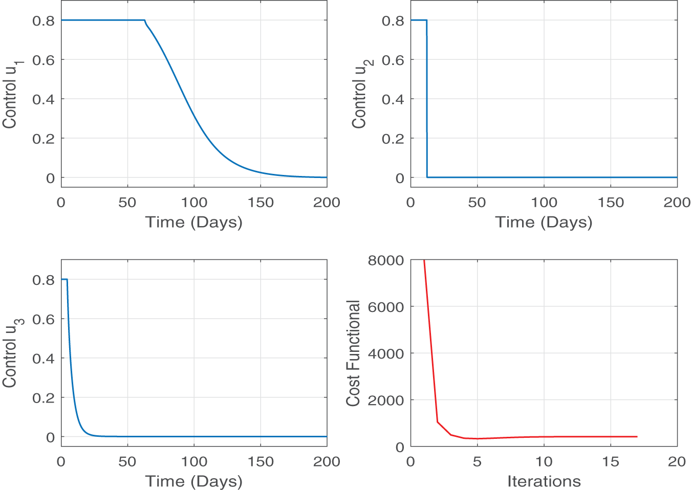
Figure 6: Figure shows the optimal profiles for control variables and their impact on the minimization of cost functional J. All three controls begin at relatively high levels and then gradually decrease over time. This means a strong implementation of
The effect of the optimal control strategy on the different compartments of the human population is depicted in Fig. 7. Without any control measures, the susceptible population decreases more significantly due to the continuous spread of infections. However, with the implementation of the optimal control measures, a larger proportion of the human population remains susceptible, demonstrating effective disease prevention efforts. The number of people who are exposed, infected, asymptomatic, and receiving treatment is significantly decreased with controls than without, indicating a successful suppression of disease progression. In addition, we also observed a decrease in the recovered population with the optimal controls. The optimal profiles of the state variables suggest that the disease is progressing towards the disease-free state under the optimal control measures. These findings clearly highlight the positive effect of the control strategies on public health outcomes.
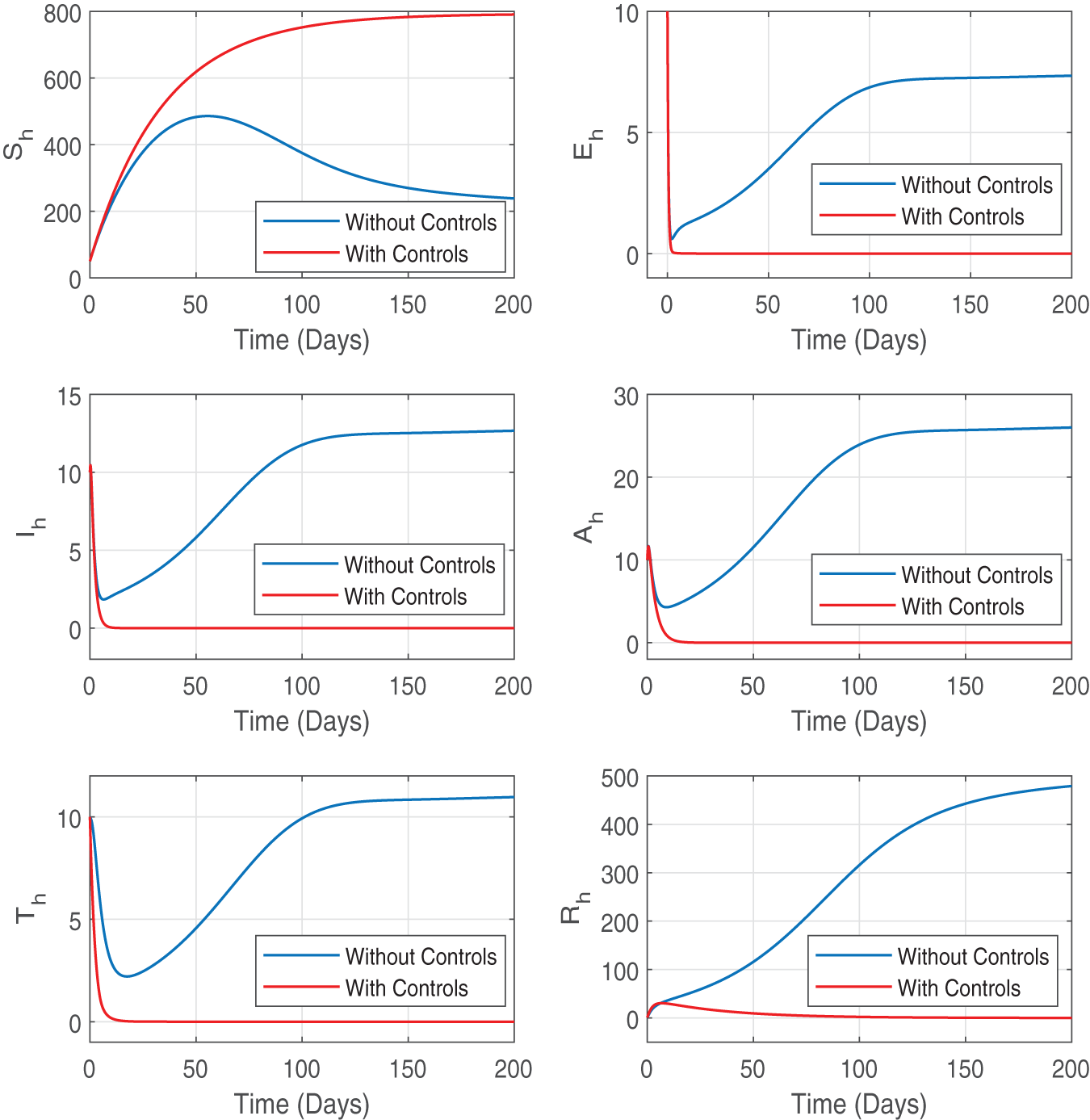
Figure 7: Figure shows the profile of state variables for the human population with and without optimal control variables. The convergence of trajectories of the optimal state variables
The impact of the control strategies on the mosquito population dynamics is illustrated in Fig. 8. The implementation of control measures results in a significant decrease in the population of susceptible, exposed, and infected mosquitoes compared to the uncontrolled scenario. Notably, the number of infected mosquitoes has observed a significant decline, which directly contributes to reducing the transmission of malaria to humans. These findings emphasize the critical role of mosquito control efforts, denoted by
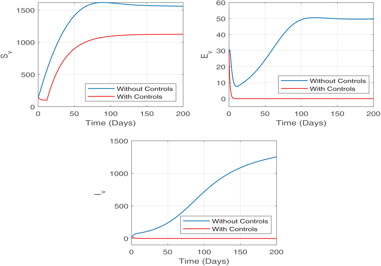
Figure 8: The impact of the control strategies on the mosquito population dynamics is illustrated in this Figure. We observe a significant decrease in the population of exposed and infected mosquitoes compared to the uncontrolled scenario
The graphical results illustrate the effectiveness and cost-efficiency of the optimal control strategy. By incorporating realistic intervention measures such as insecticide-treated nets, larvicides, and improved treatment protocols, the model accurately reflects the dynamics of the disease. The significant reduction in both disease prevalence and mosquito infection rates, achieved through moderate and gradually decreasing control measures, underscores the economic feasibility of the strategy. Furthermore, the decline in functional cost during the optimization process demonstrates that initial investments in intensive control measures can lead to substantial health improvements and long-term economic savings. In conclusion, the optimal control strategy suggested provides a valid and economically feasible method to manage and alleviate the burden of malaria.
The mathematical model developed in this study effectively captures the dynamics of malaria transmission. The model integrates asymptomatic human cases and vector populations into the traditional SEIR framework, providing a comprehensive understanding of the disease’s transmission dynamics. Through a detailed stability analysis of disease-free and endemic equilibrium points, we have identified the critical role of the basic reproduction number
The study also underscores the importance of timely and coordinated interventions. Early implementation of control measures, such as insecticide-treated nets, indoor spraying, and antimalarial drug administration, leads to the most effective reduction in transmission. A cost-effectiveness analysis suggests that combining preventive and treatment measures results in sustainable long-term malaria control. This model not only improves our understanding of the dynamics of malaria transmission but also provides practical strategies for public health authorities to implement and optimize malaria control efforts.
Some possible limitations of the model are the assumption that parameter values remain constant, the absence of spatial variability, and the exclusion of factors such as reinfection or partial immunity. Future research could introduce stochasticity and climate-related factors or different treatment regimens to further enhance its applicability in diverse settings.
Acknowledgement: We would like to thank the King Faisal University, The University of Tulsa and the University of Oklahoma for providing financial assistance.
Funding Statement: This work was supported by the Deanship of Scientific Research, Vice Presidency for Graduate Studies and Scientific Research, King Faisal University, Saudi Arabia [Grant No. KFU252959]. We are also thankful to The University of Tulsa and the University of Oklahoma for providing financial assistance.
Author Contributions: The authors confirm contribution to the paper as follows: Azhar Iqbal Kashif Butt: Conceptualization, Data curation, Formal analysis, Software, Validation, Writing—original draft, Project administration, resources. Tariq Ismaeel: Supervision, Data curation, Formal analysis, Investigation, Project administration, Resources, Writing—review & editing. Sara Khan: Conceptualization, Writing—original draft, Data curation, Formal analysis, Investigation. Muhammad Imran: Software, Validation, Visualization, Writing—review & editing. Waheed Ahmad: Formal analysis, Investigation, Validation, Visualization, Writing—review & editing. Ismail Abdulrashid: Data curation, Visualization, Project administration, Writing—review & editing. Muhammad Sajid Riaz: Software, Data curation, Project administration, Writing—review & editing. All authors reviewed the results and approved the final version of the manuscript.
Availability of Data and Materials: Data sharing not applicable to this article as no datasets were generated or analyzed during the current study.
Ethics Approval: Not applicable.
Conflicts of Interest: The authors declare no conflicts of interest to report regarding the present study.
Use of AI Tools Declaration: The authors utilized ChatGPT AI to refine the language and enhance the clarity of this manuscript. All content was thoroughly reviewed and edited to ensure accuracy, and the authors take full responsibility for the final publication.
References
1. Haringo AT, Obsu LL, Bushu FK. A mathematical model of malaria transmission with media-awareness and treatment interventions. J Appl Math Comput. 2024;70(5):4715–53. doi:10.1007/s12190-024-02154-9. [Google Scholar] [CrossRef]
2. Duve P, Charles S, Munyakazi J, Lühken R, Witbooi P. A mathematical model for malaria disease dynamics with vaccination and infected immigrants. Math Biosci Eng. 2024;21(1):1082–109. doi:10.3934/mbe.2024045. [Google Scholar] [PubMed] [CrossRef]
3. Mojeeb A, Adu IK, Yang C. A simple SEIR mathematical model of malaria transmission. Asian Res J Math. 2017;7(3):1–22. doi:10.9734/arjom/2017/37471. [Google Scholar] [CrossRef]
4. Imran M, McKinney BA, Butt AI, Palumbo P, Batool S, Aftab H. Optimal control strategies for dengue and malaria co-infection disease model. Mathematics. 2024;13(1):43. doi:10.3390/math13010043. [Google Scholar] [CrossRef]
5. Crutcher JM, Hoffman SL. Malaria. In: Baron S, editor. Medical Microbiology. 4th edition. Galveston, TX, USA: University of Texas Medical Branch at Galveston; 1996. [Google Scholar]
6. White NJ. Determinants of relapse periodicity in Plasmodium vivax malaria. Malar J. 2011;10(1):297. doi:10.1186/1475-2875-10-297. [Google Scholar] [PubMed] [CrossRef]
7. Yunus AO, Olayiwola MO. Mathematical modeling of malaria epidemic dynamics with enlightenment and therapy intervention using the Laplace-Adomian decomposition method and Caputo fractional order. Franklin Open. 2024;8(1):100147. doi:10.1016/j.fraope.2024.100147. [Google Scholar] [CrossRef]
8. Yunus AO, Olayiwola MO. The analysis of a co-dynamic ebola and malaria transmission model using the Laplace Adomian decomposition method with Caputo fractional-order. Tanz J Sci. 2024;50(2):204–43. doi:10.4314/tjs.v50i2.5. [Google Scholar] [CrossRef]
9. Abdulrashid I, Han X. A mathematical model of chemotherapy with variable infusion. Commun Pure Appl Anal. 2020;19(4):1875–90. [Google Scholar]
10. Abdulrashid I, Friji H, Topuz K, Ghazzai H, Delen D, Massoud Y. An analytical approach to evaluate the impact of age demographics in a pandemic. Stoch Environ Res Risk Assess. 2023;37(10):3691–705. doi:10.1007/s00477-023-02477-2. [Google Scholar] [PubMed] [CrossRef]
11. Mandal S, Sarkar RR, Sinha S. Mathematical models of malaria—a review. Malar J. 2011;10(1):202. doi:10.1186/1475-2875-10-202. [Google Scholar] [PubMed] [CrossRef]
12. Chiyaka C, Tchuenche JM, Garira W, Dube S. A mathematical analysis of the effects of control strategies on the transmission dynamics of malaria. Appl Math Comput. 2008;195(2):641–62. doi:10.1016/j.amc.2007.05.016. [Google Scholar] [CrossRef]
13. Ngwa GA, Shu WS. A mathematical model for endemic malaria with variable human and mosquito populations. Math Comput Model. 2000;32(7–8):747–63. doi:10.1016/s0895-7177(00)00169-2. [Google Scholar] [CrossRef]
14. Karaoglu S, Imran M, McKinney BA. Network-based SEITR epidemiological model with contact heterogeneity: comparison with homogeneous models for random, scale-free and small-world networks. Eur Phys J Plus. 2025;140(6):551. doi:10.1140/epjp/s13360-025-06481-z. [Google Scholar] [CrossRef]
15. Ferraccioli F, Riccetti N, Fasano A, Mourelatos S, Kioutsioukis I, Stilianakis NI. Effects of climatic and environmental factors on mosquito population inferred from West Nile virus surveillance in Greece. Sci Rep. 2023;13(1):18803. doi:10.1038/s41598-023-45666-3. [Google Scholar] [PubMed] [CrossRef]
16. Beck-Johnson LM, Nelson WA, Paaijmans KP, Read AF, Thomas MB, Bjørnstad ON. The effect of temperature on Anopheles mosquito population dynamics and the potential for malaria transmission. PLoS One. 2013;8(11):e79276. doi:10.1371/journal.pone.0079276. [Google Scholar] [PubMed] [CrossRef]
17. Imran M, Butt AI, McKinney BA, Al Nuwairan M, Al Mukahal FH, Batool S. A comparative analysis of different fractional optimal control strategies to eradicate Bayoud disease in date palm trees. Fractal Fract. 2025;9(4):260. doi:10.3390/fractalfract9040260. [Google Scholar] [CrossRef]
18. Yunus AO, Olayiwola MO. Epidemiological analysis of Lassa fever control using novel mathematical modeling and a dual-dosage vaccination approach. BMC Res Notes. 2025;18(1):199. doi:10.1186/s13104-025-07218-y. [Google Scholar] [PubMed] [CrossRef]
19. Imran M, McKinney B, Butt AI. SEIR mathematical model for influenza-corona co-infection with treatment and hospitalization compartments and optimal control strategies. Comput Model Eng Sci. 2025;142(2):1899–931. doi:10.32604/cmes.2024.059552. [Google Scholar] [CrossRef]
20. Srivastav AK, Steindorf V, Stollenwerk N, Aguiar M. The effects of public health measures on severe dengue cases: an optimal control approach. Chaos Solitons Fractals. 2023;172:113577. [Google Scholar]
21. Thongtha A, Modnak C. Optimal control strategy of a dengue epidemic dynamics with human-mosquito transmission. Bur Sci J. 2017;2017:333–42. [Google Scholar]
22. Adom-Konadu A, Yankson E, Naandam SM, Dwomoh D. A mathematical model for effective control and possible eradication of malaria. J Math. 2022;2022(1):6165581. doi:10.1155/2022/6165581. [Google Scholar] [CrossRef]
23. Al Basir F, Abraha T. Mathematical modelling and optimal control of malaria using awareness-based interventions. Math. 2023;11(7):1687. doi:10.3390/math11071687. [Google Scholar] [CrossRef]
24. Al-Arydah MT, Smith R. Controlling malaria with indoor residual spraying in spatially heterogenous environments. Math Biosci Eng. 2011;8(4):889–914. doi:10.3934/mbe.2011.8.889. [Google Scholar] [PubMed] [CrossRef]
25. Traoré B, Sangaré B, Traoré S. A mathematical model of malaria transmission with structured vector population and seasonality. J Appl Math. 2017;2017(1):6754097. doi:10.1155/2017/6754097. [Google Scholar] [CrossRef]
26. Moulay D, Aziz-Alaoui MA, Cadivel M. The chikungunya disease: modeling, vector and transmission global dynamics. Math Biosci. 2011;229(1):50–63. doi:10.1016/j.mbs.2010.10.008. [Google Scholar] [PubMed] [CrossRef]
27. Burden R, Faires J. Numerical analysis. 9th ed. Boston, MA, USA: Cengage Learning; 2011. [Google Scholar]
28. Birkhoff G, Rota G. Ordinary differential equation. 4th ed. New York, NY, USA: John Wiley & Sons; 1989. [Google Scholar]
29. Van den Driessche P. Reproduction numbers of infectious disease models. Infect Dis Model. 2017;2(3):288–303. doi:10.1016/j.idm.2017.06.002. [Google Scholar] [PubMed] [CrossRef]
30. Diekmann O, Heesterbeek JA, Metz JA. On the definition and the computation of the basic reproduction ratio R0 in models for infectious diseases in heterogeneous populations. J Math Biol. 1990;28(4):365–82. doi:10.1007/bf00178324. [Google Scholar] [PubMed] [CrossRef]
31. Castillo-Chavez C, Blower S, van den Driessche P, Kirschner D, Yakubu AA. Mathematical approaches for emerging and reemerging infectious diseases: models, methods, and theory. New York, NY, USA: Springer Science & Business Media; 2002. [Google Scholar]
32. Pontryagin LS. Mathematical theory of optimal processes. London, UK: Routledge; 2018. [Google Scholar]
33. Agusto FB. Optimal chemoprophylaxis and treatment control strategies of a tuberculosis transmission model. World J Model Simul. 2009;5(3):163–73. [Google Scholar]
34. Mukhtar AY, Munyakazi JB, Ouifki R, Clark AE. Modelling the effect of bednet coverage on malaria transmission in South Sudan. PLoS One. 2018;13(6):e0198280. doi:10.1371/journal.pone.0198280. [Google Scholar] [PubMed] [CrossRef]
35. Imran M, Rafique H, Khan A, Malik T. A model of bi-mode transmission dynamics of Hepatitis C with optimal control. Theory in Biosciences. 2014;133(2):91–109. doi:10.1007/s12064-013-0197-0. [Google Scholar] [PubMed] [CrossRef]
36. Lenhart S, Workman JT. Optimal control applied to biological models. Boca Raton, FL, USA: Chapman and Hall/CRC; 2007. [Google Scholar]
Cite This Article
 Copyright © 2025 The Author(s). Published by Tech Science Press.
This work is licensed under a Creative Commons Attribution 4.0 International License , which permits unrestricted use, distribution, and reproduction in any medium, provided the original work is properly cited.
 Downloads
 Citation Tools