
 Submit a Paper
 Propose a Special lssue
 Open Access
ARTICLE

Type-I Heavy-Tailed Burr XII Distribution with Applications to Quality Control, Skewed Reliability Engineering Systems and Lifetime Data
1 Department of Statistics, Faculty of Physical Sciences, Nnamdi Azikiwe University, Awka, P.O. Box 5025, Nigeria
2 Department of Mathematics and Statistics, Faculty of Science, Imam Mohammad Ibn Saud Islamic University (IMSIU), Riyadh, 11432, Saudi Arabia
3 Department of Mathematics and Statistics, Faculty of Engineering and Applied Sciences, Riphah International University, Islamabad, 44000, Pakistan
4 Department of Statistics, School of Computer Science and Engineering, Lovely Professional University, Phagwara, 144411, Punjab, India
5 Department of Basic Sciences, Higher Institute of Administrative Sciences, Belbeis, AlSharkia, 44621, Egypt
* Corresponding Author: Okechukwu J. Obulezi. Email:
Computer Modeling in Engineering & Sciences 2025, 144(3), 2991-3027. https://doi.org/10.32604/cmes.2025.069553
Received 26 June 2025; Accepted 21 August 2025; Issue published 30 September 2025
 View Full Text
 Download PDF
Abstract
This study introduces the type-I heavy-tailed Burr XII (TIHTBXII) distribution, a highly flexible and robust statistical model designed to address the limitations of conventional distributions in analyzing data characterized by skewness, heavy tails, and diverse hazard behaviors. We meticulously develop the TIHTBXII’s mathematical foundations, including its probability density function (PDF), cumulative distribution function (CDF), and essential statistical properties, crucial for theoretical understanding and practical application. A comprehensive Monte Carlo simulation evaluates four parameter estimation methods: maximum likelihood (MLE), maximum product spacing (MPS), least squares (LS), and weighted least squares (WLS). The simulation results consistently show that as sample sizes increase, the Bias and RMSE of all estimators decrease, with WLS and LS often demonstrating superior and more stable performance. Beyond theoretical development, we present a practical application of the TIHTBXII distribution in constructing a group acceptance sampling plan (GASP) for truncated life tests. This application highlights how the TIHTBXII model can optimize quality control decisions by minimizing the average sample number (ASN) while effectively managing consumer and producer risks. Empirical validation using real-world datasets, including “Active Repair Duration,” “Groundwater Contaminant Measurements,” and “Dominica COVID-19 Mortality,” further demonstrates the TIHTBXII’s superior fit compared to existing models. Our findings confirm the TIHTBXII distribution as a powerful and reliable alternative for accurately modeling complex data in fields such as reliability engineering and quality assessment, leading to more informed and robust decision-making.Keywords
In the analysis of real-world phenomena, rare events and complex hazard behaviors are common, necessitating the use of flexible statistical distributions. Classical models such as the normal, exponential, Weibull, and Rayleigh often prove inadequate in modeling data characterized by significant skewness, heavy tails, or non-monotonic hazard functions. Consequently, the development of more versatile distributions, particularly those with heavy-tailed behavior, has been a central focus of modern applied statistics.
Heavy-tailed distributions, which allocate a higher probability mass to extreme outcomes than Gaussian models, have been observed across a wide range of disciplines. In finance, for example, asset prices and stock returns frequently exhibit fat-tailed tendencies, with the probability of large gains or losses exceeding what would be predicted by a normal distribution [1]. This has led to the adoption of stable laws to better explain high market volatility. Similarly, in actuarial science, catastrophic claims in insurance are a classic example of heavy-tailed behavior, particularly when modeling loss severity [2]. Environmental and natural systems also display these characteristics; hydrological records, rain intensities, and seismic events often follow distributions with slowly decaying tails [3,4]. In medicine and biology, skewed and extreme-value data, such as tumor sizes and survival times, similarly require heavy-tailed models for accurate analysis [5–7].
Formally, a distribution with distribution function
This implies that heavy-tailed distributions place significantly more probability mass in the tails than exponential-type distributions. Classic examples include the Cauchy distribution by Cauchy [8], Student’s
where
Among these flexible models, the Burr Type XII (BXII) distribution has been particularly influential. Introduced by Burr [21] as part of a system of distributions designed to fit a wide range of empirical data, it is a continuous probability distribution for a non-negative random variable
The ongoing demand for models capable of capturing complex data characteristics has led to a proliferation of BXII generalizations. These extensions often enhance the original BXII’s flexibility by adding new parameters or by embedding it within a larger family of distributions. For example, Gad et al. [23] introduced the Burr XII-Burr XII (BXI-BXII) distribution, a compound model that demonstrated a superior fit to certain datasets compared to the baseline BXII. The literature is rich with such constructions, which can be broadly categorized by their methodological approach.
One common strategy is the use of general families of distributions. The T-X family by Alzaatreh et al. [24], for instance, has been used to derive the Burr XII-moment exponential (BXII-ME) distribution, which offers greater flexibility for modeling lifetime data [25]. Similarly, the Kumaraswamy-G family has led to the Kumaraswamy Burr XII (KBXII) distribution, a four-parameter model with a remarkable ability to accommodate diverse functional shapes and hazard rate behaviors [26]. Another important approach involves the Marshall-Olkin extended family, which produced the Marshall-Olkin extended Burr Type XII (MOEBXII) distribution to provide enhanced flexibility for reliability and survival analysis [27]. For more details see [28–30] as well as [31–33].
Other specialized extensions of the BXII distribution have been developed to address specific challenges. Ocloo [34] introduced a novel extension of the Burr XII distribution, demonstrating its enhanced capability to model data with complex characteristics such as bimodality and heavy tails, and providing a better fit than many existing BXII extensions. Recent innovations also include the Sine-Burr XII distribution, which utilizes a trigonometric transformation to add flexibility without introducing new parameters [35], and the Odd Burr XII Gompertz (OBXIIGo) distribution, which provides a more adaptable model for lifetime data by integrating the BXII family with the Gompertz distribution [36].
The work of Gad et al. [23] and other similar studies underscore a critical motivation in modern statistical modeling: the development of new distributions that can effectively capture complex data structures not adequately described by classical models. The literature reviewed herein indicates a clear trend toward creating higher-order BXII-based models that offer greater flexibility in their distributional shapes and hazard rate functions. These models consistently serve as a better alternative to their classical counterparts, a finding supported by statistical goodness-of-fit metrics.
One such area where the choice of distribution is paramount is in acceptance sampling, particularly within truncated life-testing experiments. In specialized manufacturing or medical diagnosis, using simple, stratified, or cluster sampling may be insufficient. Group acceptance sampling plans (GASPs) provide an efficient alternative by examining several units in batches, conserving resources. The efficacy of a GASP, however, hinges on the choice of the underlying product lifetime distribution. An ill-suited model can lead to misclassifying good or bad lots, resulting in either excessive consumer risk or uneconomical producer rejection. This has prompted researchers to propose GASPs under more generalized distributions to overcome the limitations of standard models. For example, GASPs have been developed for truncated life tests based on the inverse Rayleigh and log-logistic distributions by Aslam & Jun [37], the Marshall-Olkin extended Lomax distribution by Rao [38], and the inverse Weibull distribution with median lifetime as a quality measure by Singh & Tripathi [39]. Other recent studies have employed generalized distributions like the AG-transmuted exponential by Almarashi & Khan [40], transmuted exponential by Owoloko et al. [41], transmuted Rayleigh by Saha et al. [42], and exponential-logarithmic distributions by Ameeq et al. [43] in the GASP framework. This body of research demonstrates that superior modeling of the lifetime distribution directly leads to more efficient and risk-balanced sampling decisions. Most recently, Ekemezie et al. [44] presented the odd Perks-Lomax (OPL) distribution and used it to construct a GASP, showcasing how a novel, versatile distribution can enhance both statistical theory and practical application simultaneously.
Building on this demonstrated need for more intricate models, this research proposes and thoroughly investigates a novel statistical distribution: the Type-I Heavy-Tailed Burr Type XII (TIHTBXII) distribution. The primary motivation is to address the persistent challenges in adequately modeling real-world data with extreme skewness, heavy tails, and complex, non-monotonic hazard functions, for which existing generalized distributions still exhibit limitations. We not only meticulously derive the mathematical properties of the TIHTBXII distribution and examine various parameter estimation procedures but, more significantly, we demonstrate its practical utility by constructing a group acceptance sampling plan (GASP) specifically tailored to truncated life tests based on this new model. This new tool leverages the TIHTBXII distribution’s excellent capability to provide more accurate and reliable data, thereby enabling better decision-making in fields like quality control, reliability engineering, and lifetime data analysis, where current models may fail to capture the true underlying risk mechanisms.
The rest of this paper is organized as follows: In Section 2, we define the basic functions of the proposed TIHTBXII model, including its probability density function (PDF), cumulative distribution function (CDF), survival function, and hazard function. Section 3 is dedicated to the derivation of several key characteristics of the TIHTBXII model, such as its quantile function, moments, incomplete moments, moment-generating function, mean residual life function, entropy, extropy, and order statistics. In Section 4, we discuss the estimation of the model parameters using maximum likelihood, maximum product spacing, least squares, and weighted least squares methods. Section 5 presents a Monte Carlo Markov Chain (MCMC) simulation study conducted with four different parameter settings, with the bias and root mean square error (RMSE) also plotted to support the numerical results. In Section 6, we design a group acceptance sampling plan (GASP) to illustrate how the TIHTBXII model can optimize quality control decisions by minimizing the average sample number. Finally, Section 7 reports the applications of the proposed model to real datasets, including the duration of active repairs of airborne communication transceivers, groundwater contaminant measurements, and Dominica COVID-19 mortality rate data, while Section 8 provides the conclusion of this study.
2 Development of the Type-I Heavy-Tailed Burr XII Distribution
The Burr XII distribution has cumulative distribution function (CDF) and probability density function (PDF), respectively, given as
and
Reference [45] proposed the Type I heavy-Tailed (TI-HT) family of distributions with CDF and PDF respectively given as
and
where
and
The survival function is
The hazard function is
The proposed TIHTBXII distribution aims to improve model flexibility, provide the best fit to real-world data, and accommodate heavy-tailed data in fields such as reliability engineering, medical and financial sciences, among others.
Fig. 1a and b represents the graph of the PDF and hazard function, respectively. These plots are at various combination of the parameter values. The plots reflect left-skewed behaviour, both low and high peaks, and bumped-shape. This demonstrate that the TIHTBXII can be utilized in modeling different lifetime events. The hazard rate plots depict bump-shape, bathtub, L-shape, J-shape and strictly non-decreasing shape. This again implies that TIHTBXII model can benefit from modeling different lifetime events.
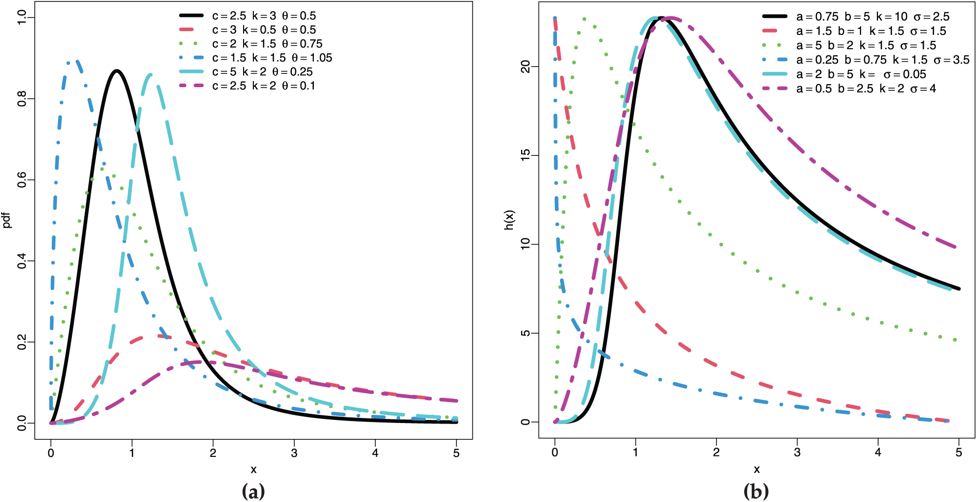
Figure 1: Plots of (a) PDF, (b) Hazard function of the TIHTBXII distribution
3 Characterization of the TIHTBXII Model
In this section, we study some basic properties of the new distribution which include quantile function, moment and incomplete moment, moment generating function, order statistic, entropy and extropy, and the mean residual life function.
The quantile function
In inference, the advantage of
The
Using series expansion
For
Also, for
Similarly,
By back substitution,
Notice that
so that
Therefore,
For a continuous random variable
Substitute into the incomplete moment:
Using the generalized binomial expansion:
Expanding the second term yields
and
Also,
The integrand becomes a power series in
Now collect all powers of
Hence,
3.4 Moment Generating Function
Let
Using series expansion
For
Also, for
Similarly,
By back substitution,
Notice that
so that
Therefore,
3.5 Mean Residual Life Function
The mean residual life (MRL) function of a non-negative continuous random variable X is defined as
where
Recall that for
hence
Similarly, by expanding
Also, by expanding
Recall
Therefore, the MRL function is
Entropy is a fundamental concept in information theory and statistical mechanics, used to quantify the uncertainty or randomness associated with a probability distribution. For a given probability density function
In this section, we derive the Rényi entropy of the proposed distribution. Due to the complexity of the density function, the integral involved is analytically intractable in closed form. However, by applying the generalized binomial expansion and power series techniques, we express the entropy in terms of infinite series and known special functions, particularly the Gamma function.
Using generalized binomial expansion when
Similarly,
Therefore,
Recall that
This subsection defines extropy, a measure of order or information content within a system, serving as a dual to the more commonly known concept of entropy. We consider a specific mathematical formulation of extropy, denoted by the functional
Using generalized binomial expansion; for
Also,
Similarly,
So that,
Since,
In the realm of probability theory and statistics, an order statistic is a fundamental concept representing the
We proceed with the estimation of the parameters of the TIHTBXII distribution using maximum likelihood, maximum product spacing, least squares and weighted least squares procedures.
4.1 Maximum Likelihood Estimation
Maximum Likelihood Estimation (MLE) involves finding the values of the parameters that maximize the likelihood of observing the given data. First, we formulate the likelihood function. Let
Formulate the log-likelihood function since it is almost always easier to work with the natural logarithm of the likelihood function, called the log-likelihood function, denoted as
and
Next, solve the system of score equations. The MLEs for
The solutions can be obtained numerically.
4.2 Maximum Product Spacing Estimation
The Maximum Product Spacing (MPS) method estimates parameters by maximizing the product of the differences between consecutive values of the CDF, evaluated at ordered observations. Let
for
Alternatively, it is often more convenient to maximize the logarithm of the product spacing function:
The MPS estimates
The Least Squares (LS) method estimates parameters by minimizing the sum of squared differences between the empirical CDF and the theoretical CDF. Let
To find the estimates, we set the partial derivatives of
These equations are typically solved numerically.
4.4 Weighted Least Squares Estimation
Weighted Least Squares (WLS) is an extension of LS that incorporates weights to account for varying precision across observations. In the context of empirical CDF fitting, weights are often chosen to reflect the variance of the ordered statistics. The WLS estimates
A common choice for weights
The system of equations to solve for the WLS estimates is:
Numerical optimization is required to solve this system. To implement the LS and WLS methods, the partial derivatives of
To contrast the performance of the estimation methods (MLE, MPS, LS, and WLS), we conduct a Monte Carlo Markov Chain (MCMC) simulation study. In the simulation, we test the bias and root mean square error (RMSE) of the parameter estimates for various sample sizes and true parameter values. MCMC simulation is a powerful and widely used approach for evaluating the efficiency of estimators, particularly for advanced statistical models in which analytical solutions are impossible, based on early work by Metropolis et al. [46] and then subsequently broadened by Hastings [47].
For our computation, we performed 1000 Monte Carlo repetitions for each of the scenarios and sample sizes. In each of these, we generated data from the TIHTBXII distribution, via its quantile function, from uniformly distributed random numbers. Numerical optimization (with in particular optim in R) was used to estimate MLE, LS, and WLS parameters, while the MPS estimates were calculated using the function mpsedist from the package BMT.
Our simulation experiment is done on the basis of four distinct scenarios, which are equivalent to different combinations of the distribution parameters
Scenario I
Scenario II
Scenario III
Scenario IV
For each situation, we generate random samples of varying sizes (
The simulation results, which are reported in Tables 1 and 2, provide information about the performance of the MLE, MPS, LS, and WLS estimators of the parameters of the TIHTBXII distribution for various sample sizes and settings. The overall pattern in all the methods and settings is that Bias and Root Mean Square Error (RMSE) decrease as the sample size increases. This demonstrates that all estimators are more precise and accurate with larger data. Estimation of
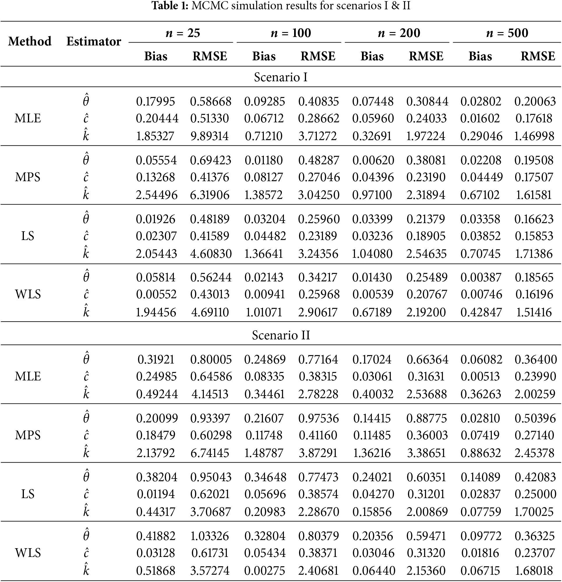
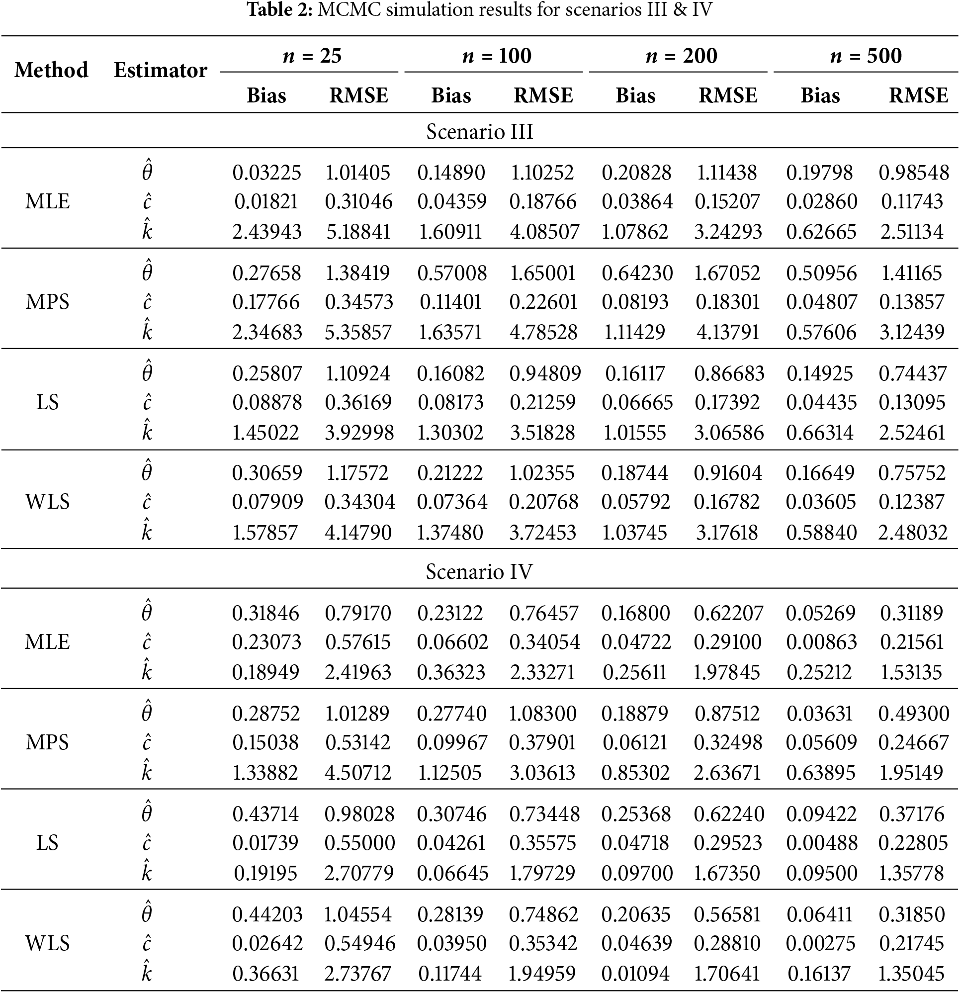
Scenario-dependent results show that the parameter values chosen influence estimation challenge. For instance, Scenario I is “easier” to estimate with lower overall RMSE values, whereas Scenarios II and IV are challenging, particularly for
Fig. 2a and b is the plots of the Bias and RMSE of the four non-Bayesian methods for Scenarios I and II while Fig. 3a and b is the plots of the Bias and RMSE of the four non-Bayesian methods for Scenarios III and IV. These support the numerical results in Tables 1 and 2 since as the sample size increases, the Bias remain positive and the RMSE decrease. These are indicators of good convergence behavior which indicate that the TIHTBXII model is fit for modeling lifetime datasets.
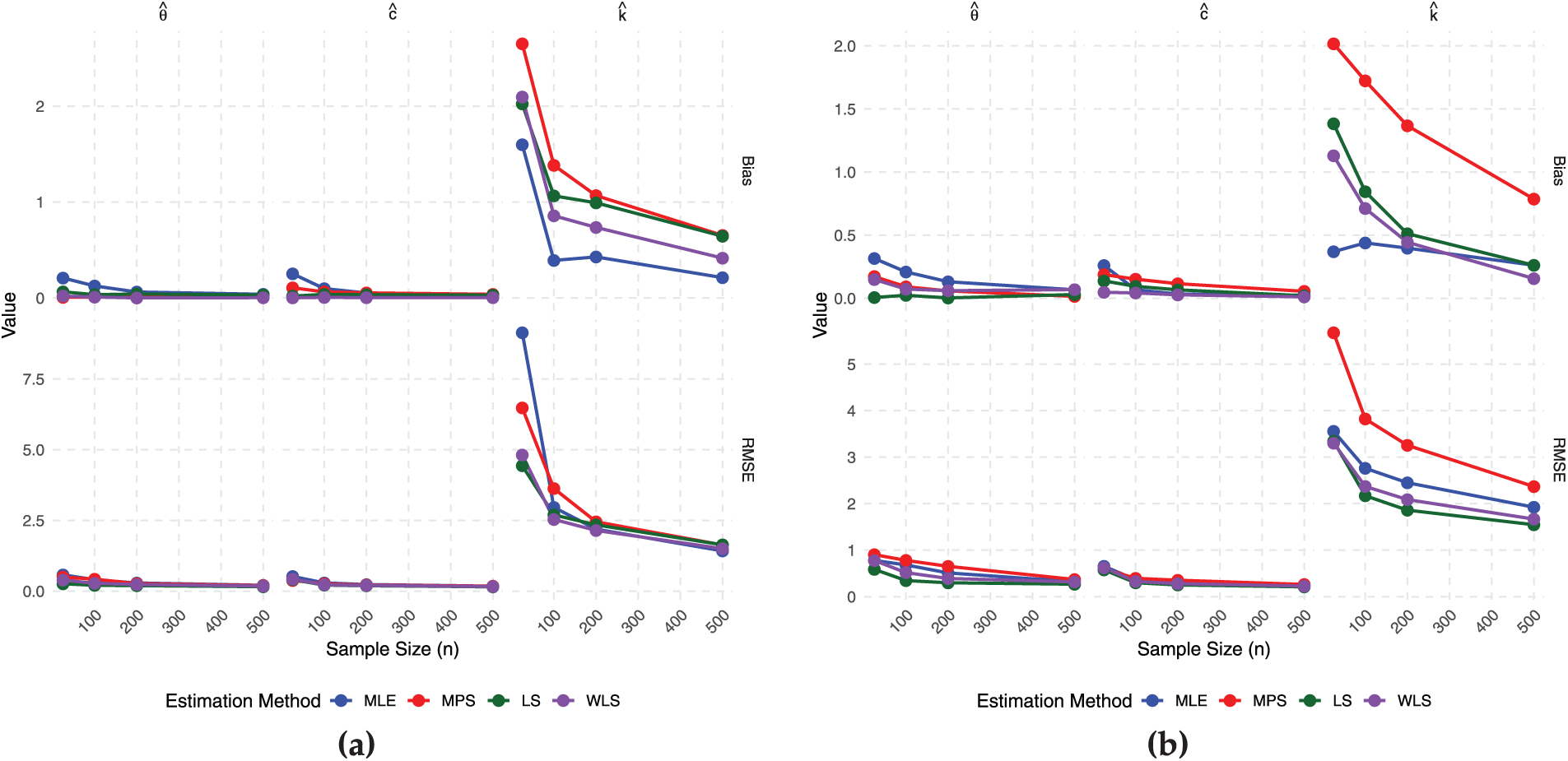
Figure 2: Estimator performance (a) scenario I (b) scenario II
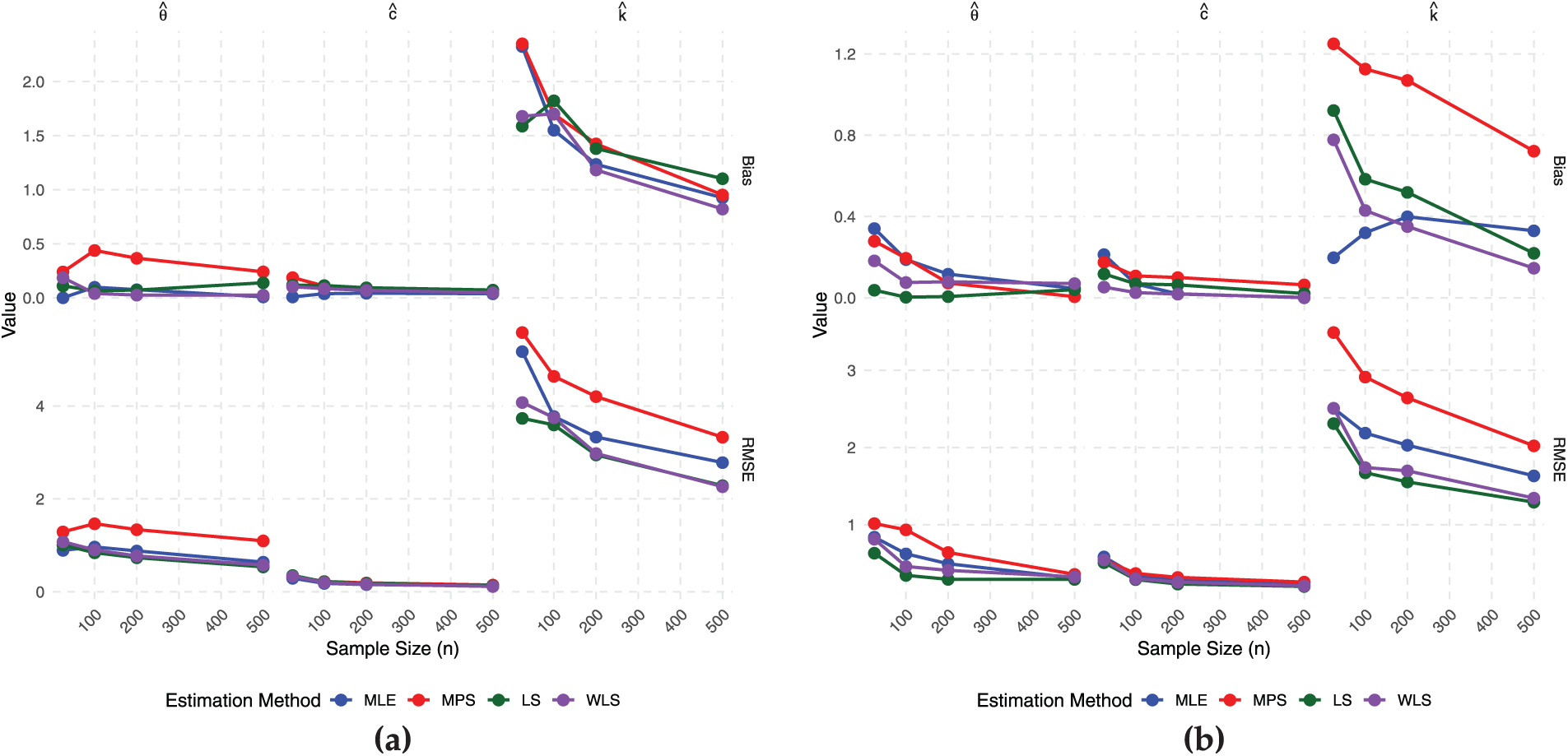
Figure 3: Estimator performance (a) scenario III (b) scenario IV
6 GASP Based on Truncated Life Tests for TIHTBXII Distribution
This section presents the use of Group Acceptance Sampling Plan (GASP) in truncated life tests for items having lifetimes that are TIHTBXII-distributed. Truncated life tests are very important for effective quality control, particularly in the case of testing long-lifetime components. The median lifetime of an item with TIHTBXII-distributed lifetime is obtained using its quantile function, given in Eq. (9). For the median (
For ease of calculations under the GASP platform, we split
This split is such that
For the truncated life tests, the test duration is provided by
The failure probability,
This expression for
The GASP design parameters, i.e., the number of groups (G), the acceptance number (
Here,
Table 3 presents an illustrative set of GASP design parameters for the TIHTBXII distribution, based on specific parameter values (
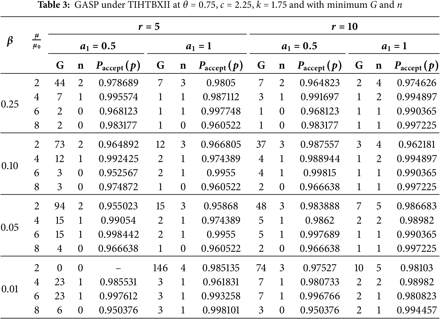
The factors influencing the optimal plan are:
(a)
(b)
(c)
(d)
The triplet given
(i) Mean Ratio Influence (
For example, for
This means that more inspection repetitions enable a more effective sampling plan with fewer groups or items in each run needed to get the required acceptance probability.
(ii) Impact of the truncation time scaling factor (
The trend, while generally generating more frugal plans, will be at the expense of G or
(iii) Non-Feasible Plans (
The
Fig. 4a–d is the operating characteristic (OC) curve for

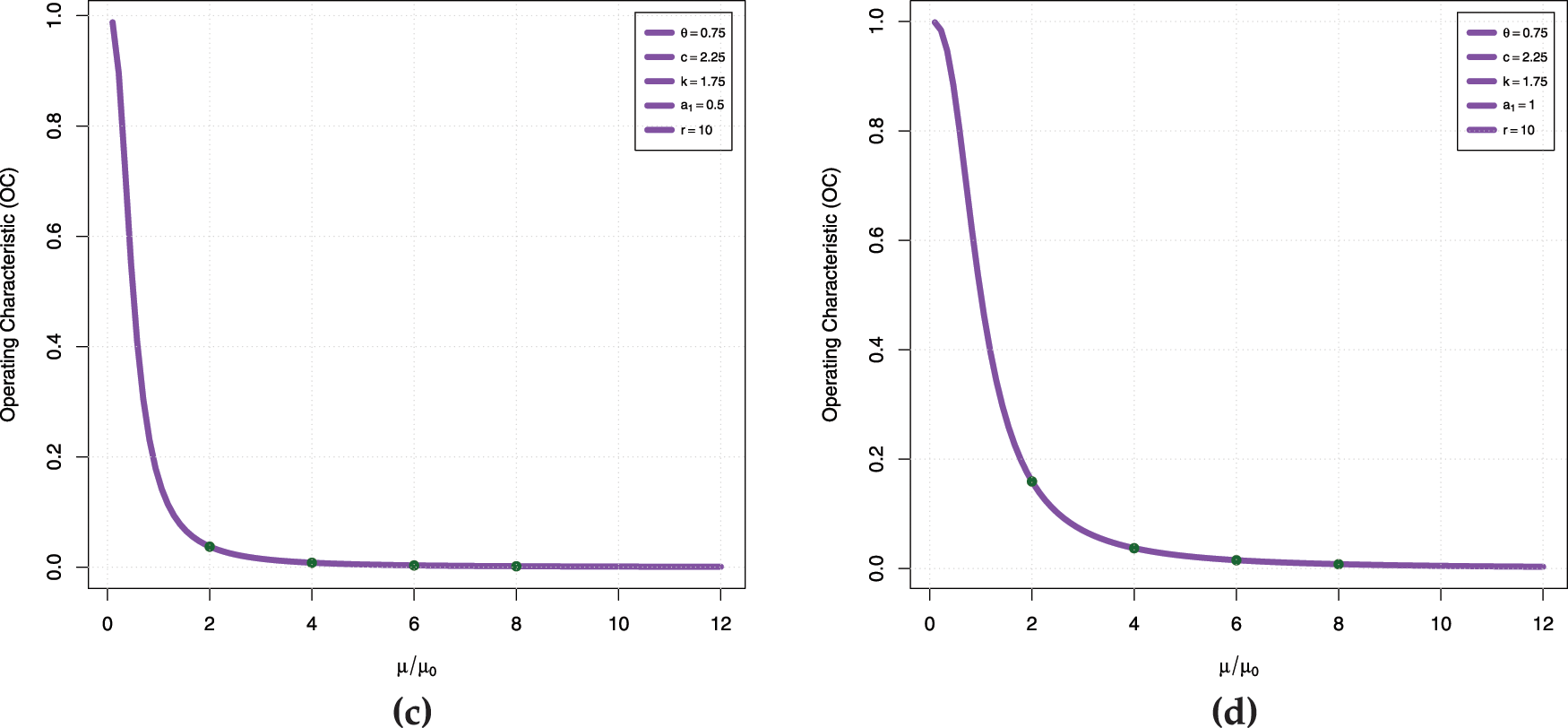
Figure 4: OC curve (a) case I (b) case II (c) case III (d) case IV
Case I:
Case II:
Case III:
Case IV:
Table 4 provides the optimum parameters

Each triplet
(i) Influence of Mean Ratio (
(ii) Consumer’s Risk (
(iii) Impact of Repetition Factor (
For example, for
(iv) Effect of Truncation Time Scaling Factor (
This indicates that having a relatively longer test duration (
(v) Non-Feasible Plans (
The accept values of
Fig. 5a–d is the operating characteristic (OC) curve for Case I, Case II, Case III and Case IV, respectively, based on
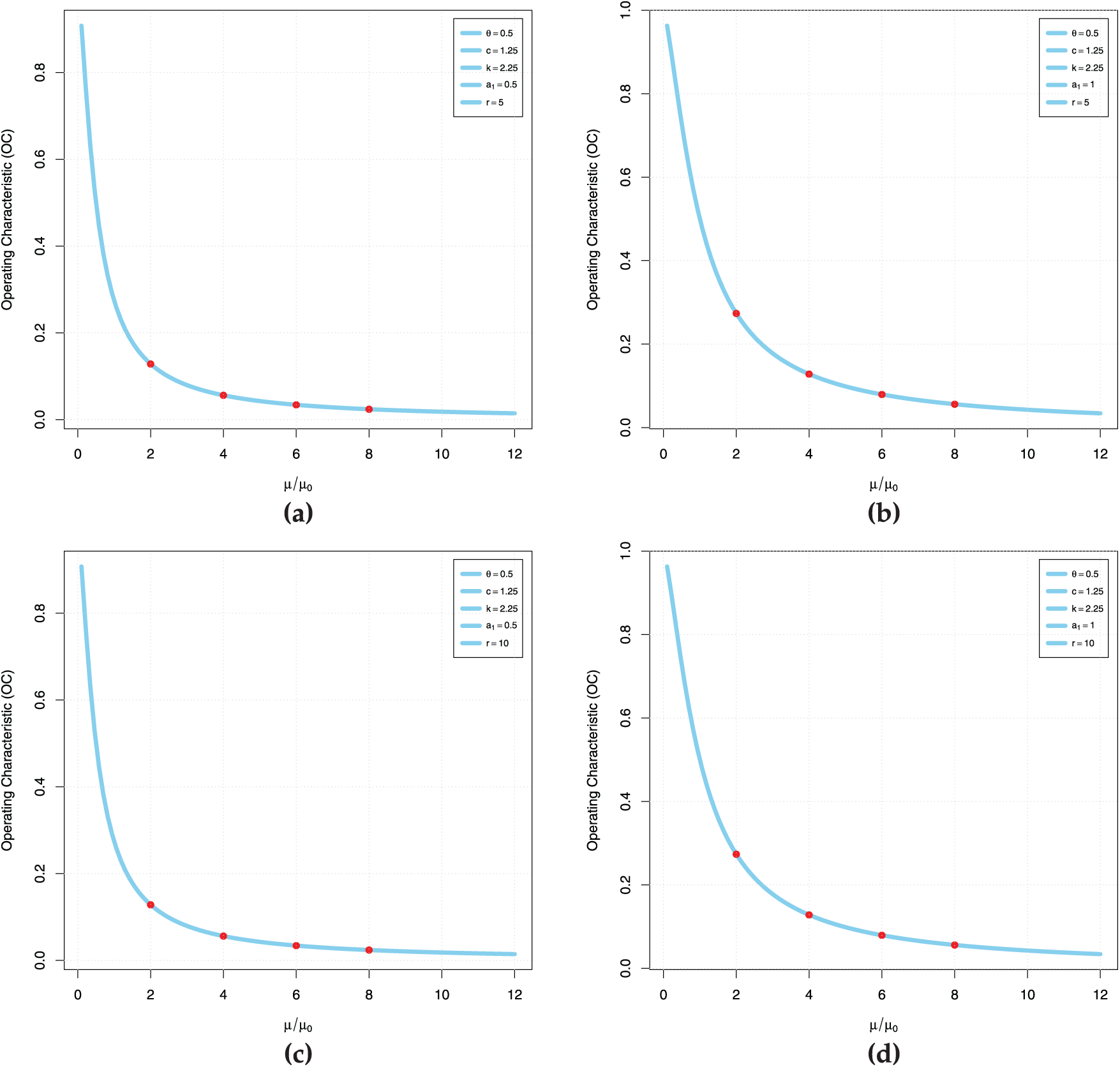
Figure 5: OC curve for
The first data to be used for illustrating the importance of the TIHTBXII model is the duration of active repairs for airborne communication transceivers. This data was studied by El-Saeed et al. [48] and Mead et al. [49] and presented in Table 5.

The second application data is related to groundwater contaminants measurements taken to monitor and assess the effectiveness of environmental cleanup efforts. It has been studied by Bhaumik et al. [50] and contained in Table 6, clean-up-gradient monitoring wells, expressed in milligrams per liter (mg/L).

Weekly Death rate due to COVID-19 from 22/3/2020 to 20/12/2020 in Dominica retrieved from https://data.who.int/dashboards/covid19/data?n=c (accessed on 20 August 2025) and reported in Table 7 below.

We present a table of summary statistics with important measures such as the

Table 8 brings together three different data sets, showing a similar pattern of positive skewness in each. This means each data set holds more small values and a tail that extends to high values due to occasional gigantic observations or outliers. The Active Repair Duration data is the most skewed and dispersed, and it accounts for many short repairs but also for every now and then a very long one, as indicated by its very high skewness (2.7171) and kurtosis (10.5433). Groundwater Contaminant Measurements also show clear right-skewness (1.6037), indicating that most measurements are low but with the periodic high contaminant levels pulling the average quite high. Lastly, Dominica COVID-19 Mortality data, though still positively skewed (1.0777), is the most compact and least spread out with only outliers at higher mortality rates.
Fig. 6 contains boxplots superimposed on the violin plots for the three datasets, respectively. The image provide evidence that the three datasets contains outliers.

Figure 6: Boxplot superimposed on violin plots
Fig. 7 contains the density plots sumperimposed on the histogram of the respective datasets. All three show positive skewness.
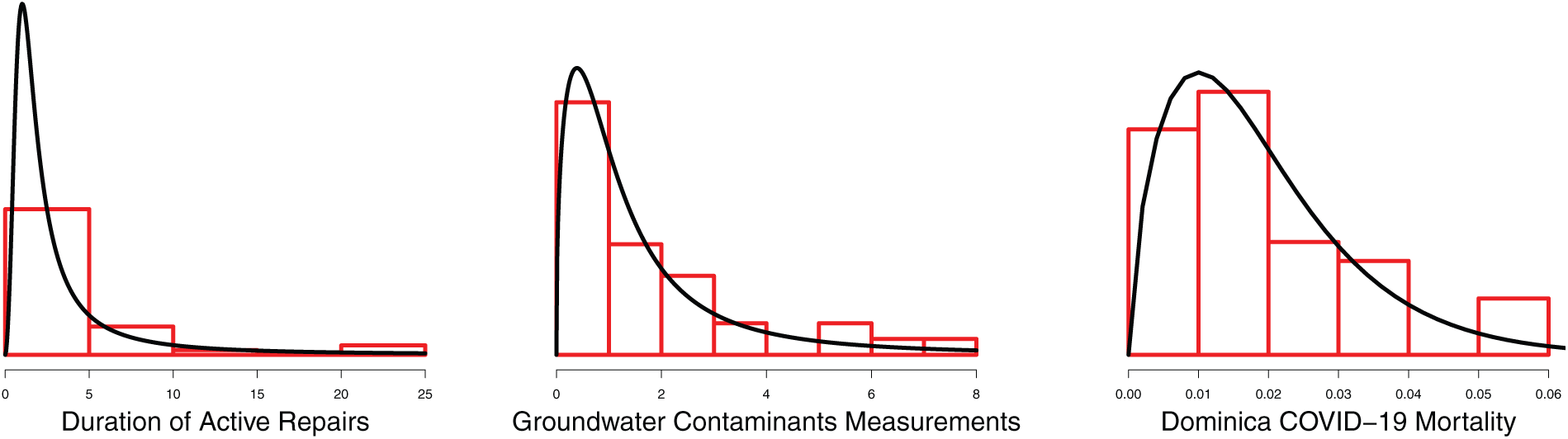
Figure 7: Kernel density superimposed on histogram
Figs. 8 and 9 are the TIHTBXII CDF and survival functions with those of the empirical from the datasets. These reflect the degree of fit of the proposed TIHTBXII to the various datasets.
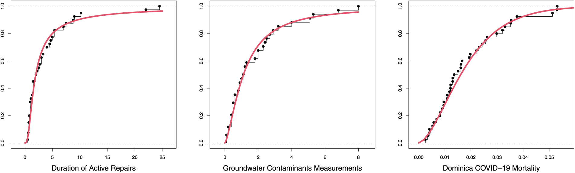
Figure 8: Empirical with TIHTBXII CDF
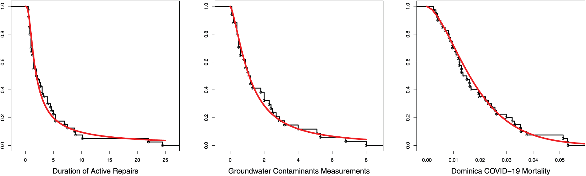
Figure 9: Empirical with TIHTBXII survival functions
Fig. 10 is the total time on test plot. The duration of active repairs and the groundwater contaminants measurements data show convex upwards TTT plots. These indicate a decreasing hazard rate (DHR). That is, as time goes on, the probability of failure for a surviving item decreases. This is often seen in early life failures where “weak” items fail quickly, leaving stronger ones. However, the Dominica COVID-19 mortality rate shows concave upward TTT plot. This indicates an increasing hazard rate (IHR). That is, as time goes on, the probability of failure for a surviving item increases.
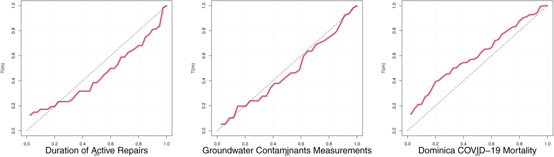
Figure 10: TTT plots
Fig. 11 is the P-P plots. For the three datasets, the P-P plots showed S-shapes or curved patterns that which indicate differences in skewness or kurtosis.
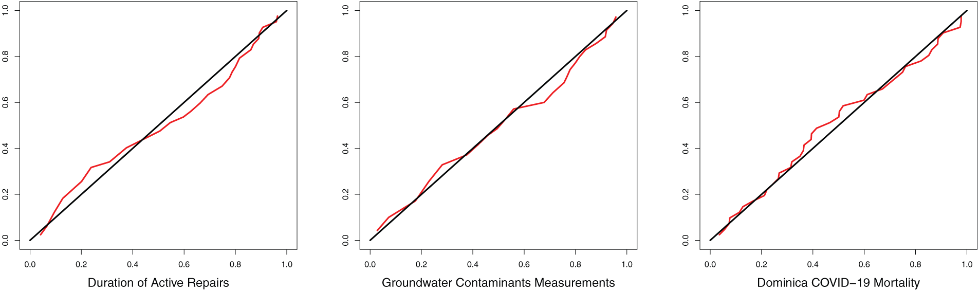
Figure 11: P-P plots
Fig. 12 is the Q-Q plots. For the groundwater contaminants measurements and the Dominica COVID-19 mortality rate, the Q-Q plots curved upwards at both ends (S-shape). These indicate heavier tails (more extreme values) in data than the TIHTBXII distribution. Hence, the datasets have higher kurtosis.
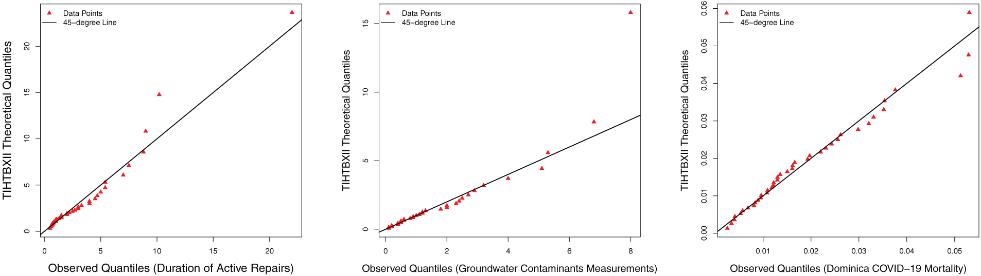
Figure 12: Q-Q plots
Figs. 13–15 are the contour plots for the three datasets. Each is a combination of any two of the parameters. The plots suggest the optimal points of the likelihood function which are contained in the MLEs table in Table 9.
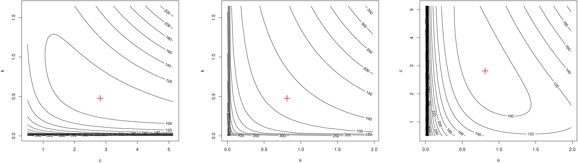
Figure 13: Contour plots for duration of active repairs

Figure 14: Contour plots for groundwater contaminants measurements

Figure 15: Contour plots for Dominica COVID-19 mortality

The choice of competing distributions are the baseline distribution being modified which is Burr type XII (BXII) distribution by Burr [21], Kumaraswamy bell-Rayleigh (KwBR) distribution by Nadir et al. [51], Gamma distribution by Johnson et al. [52], Weibull distribution by [53], Gumbel distribution by Weibull [54] and Pareto I and III by Arnold [12].
Table 10 compares a number of statistical distributions for best fit for three datasets: “Duration of Active Repairs,” “Groundwater Contaminant Measurements,” and “Dominica COVID-19 Mortality.” Comparison is by information criteria (Log-Lik, AIC, CAIC, BIC, HQIC) where lower values are preferable, and goodness-of-fit tests (W, A, D, and their p-values) where higher p-values (ideally

For the Active Repairs Duration data, the KwBR distribution, despite seemingly good information criteria, is definitively a poor fit due to its extremely low p-value (
For Groundwater Contaminants Measurements, the KwBR distribution again has a very poor fit with a null p-value. The Gamma and Weibull distributions and TIHTBXII provide the best fits, which are reinforced by their competitive information criteria and high p-values, suggesting that these models adequately describe the features of the data. The Pareto I distribution is a very poor fit for this data, as indicated by its high AIC and an extremely low p-value of 0.0017. In contrast, the Pareto III distribution is an excellent fit, with a low AIC and the highest p-value (0.9779) among all tested distributions, making it a very strong candidate for this dataset.
While comparable standard errors might make the additional parameter of TIHTBXII seem less useful, its real value is that it can provide a better fit for datasets that have more complex and highly skewed distributions. The “Duration of Active Repairs” data provides a particular case where, even with the penalty for an extra parameter, the TIHTBXII outperformed the BurrXII on the key goodness-of-fit measures. This is an indication that the extra parameter is not superfluous; it is capturing valuable information on the data structure that the simpler BurrXII model cannot capture effectively. The benefit of TIHTBXII is not always the best model, but its additional flexibility, so that it is a more viable choice for a larger array of highly skewed data from the real world, such as a hypothetical time series of volatile stock returns.
Finally, for the Dominica COVID-19 Mortality Data, the Gamma Distribution is by far the most appropriate model. It has the lowest information criteria and a high p-value (0.9157), highly indicating its suitability. Other distributions like TIHTBXII and BXII also yield good fits. The Pareto I distribution performs very poorly, with a high AIC and a p-value of 0.0007. The Pareto III distribution, however, provides a very good fit, with an excellent p-value of 0.9266 and competitive information criteria, making it a strong contender for this dataset. Again, the TIHTBXII has the best fit in the duration of active repairs data.
Table 10 provides the Maximum Likelihood Estimates (MLEs) of the parameters of various statistical distributions fitted to three data sets: “Duration of Active Repairs,” “Groundwater Contaminant Measurements,” and “Dominica COVID-19 Mortality.” Along with each MLE, in parentheses, is its standard error, a measure of the precision of the estimate; smaller standard errors indicate more precise estimates. For the Duration of Active Repairs data, the parameter estimates vary considerably across distributions. The BXII distribution, for instance, estimates the parameters c as 2.9725 and k as 0.3383, both of which have relatively small standard errors, suggesting stable estimates. Similar results were obtained for the proposed TIHTBXII distribution. For the Pareto distributions, Pareto I yields an
In this study, we introduced the Type-I Heavy-Tailed Burr Type XII (TIHTBXII) distribution as a highly flexible and robust statistical model. Our primary motivation was to address the limitations of conventional distributions in accurately capturing the complexities of real-world data, particularly those exhibiting skewness, heavy tails, and diverse hazard behaviors, common in fields such as finance, insurance, environmental science, and reliability engineering. We meticulously defined the TIHTBXII distribution, providing its PDF and CDF, and thoroughly investigated its fundamental statistical properties, including its quantile function, moments, moment-generating function, order statistics, and entropy. These foundational elements are crucial for both theoretical understanding and practical application. A significant part of our research focused on parameter estimation, where we rigorously compared four standard methods: MLE, MPS, LS, and WLS. Our extensive Monte Carlo simulation studies consistently demonstrated the consistency of these estimators; as sample size increased, the bias and RMSE of the parameter estimates decreased for all methods. Notably, the WLS and LS procedures generally outperformed MLE and MPS, exhibiting lower bias and RMSE, which underscores their stability and robustness across various scenarios and sample sizes. While MLE and MPS improved with larger sample sizes, LS and WLS consistently proved more stable and accurate in estimation for all sample sizes and parameter values considered.
Beyond theoretical exploration and estimation, we showcased the practical utility of the TIHTBXII distribution by developing a Group Acceptance Sampling Plan (GASP) using truncated life tests. This methodology is particularly valuable for quality control and life-testing procedures involving long-lifespan products and specific failure modes. We provided a comprehensive guide for optimizing GASP design parameters (number of groups, acceptance number, group size, and test duration) by minimizing the Average Sample Number (ASN) while effectively balancing consumer and producer risks. Our research highlighted how factors such as the mean ratio, consumer’s risk, repetition factor, and truncation time scaling factor influence the stringency and efficiency of the sampling plan. The TIHTBXII distribution’s ability to realistically model lifetime data directly translates into more efficient and risk-balanced decision-making in industrial settings. Empirical validation further solidified the TIHTBXII distribution’s applicability and versatility. We successfully applied the distribution to real-world datasets, including Active Repair Duration, Groundwater Contaminant Measurements, and Dominica COVID-19 Mortality. In cases like the “Active Repair Duration” data, the TIHTBXII distribution demonstrated a superior fit compared to other established models, as supported by favorable information criteria and goodness-of-fit test statistics. This empirical evidence underscores the TIHTBXII’s potential as a valuable tool for analysts and engineers working with heavy-tailed, skewed, and complex data in reliability engineering and quality measurement.
While this study effectively demonstrates the significant potential of the TIHTBXII distribution, it’s important to acknowledge certain limitations. Our Monte Carlo simulation studies, though extensive, were conducted under specific assumptions regarding parameter values and sample sizes. The performance of estimation methods, particularly MLE and MPS, might exhibit different convergence rates or biases in scenarios with extremely small sample sizes or highly unusual parameter combinations not explored in our simulations. Second, the GASP design was developed specifically for truncated life tests. The applicability and optimality of the proposed GASP framework might vary for other life-testing scenarios, such as complete life tests or different truncation mechanisms. Finally, while the empirical applications showcased the TIHTBXII’s superior fit for the selected datasets, its generalizability and superiority across all possible heavy-tailed and skewed datasets need further validation through broader comparative studies. Future research could explore its performance with even more diverse and complex real-world data from various domains to fully ascertain its range of applicability.
In conclusion, the Type-I Heavy-Tailed Burr Type XII distribution is a robust and valuable addition to the family of statistical models. It offers enhanced flexibility and strength to accurately identify realistic data patterns, particularly for data characterized by skewness and heavy tails. Its improved parameter estimation capabilities and proven effectiveness in real-world problems like acceptance sampling make it an effective alternative to traditional distributions, ultimately leading to more reliable and accurate decisions across various scientific and engineering disciplines.
Acknowledgement: Not applicable.
Funding Statement: This work was supported and funded by the Deanship of Scientific Research at Imam Mohammad Ibn Saud Islamic University (IMSIU) (Grant Number IMSIU-DDRSP2501).
Author Contributions: Okechukwu J. Obulezi: Conceptualization, Methodology, Software, Formal Analysis, Writing—Original Draft, Writing—Review & Editing. Hatem E. Semary: Supervision, Validation, Funding Acquisition, Writing—Review & Editing. Sadia Nadir: Formal Analysis, Data Curation, Writing—Review & Editing. Chinyere P. Igbokwe: Investigation, Visualization, Resources, Writing—Original Draft. Gabriel O. Orji: Methodology, Data Curation, Project Administration. A. S. Al-Moisheer: Validation, Data Curation, Writing—Review & Editing. Mohammed Elgarhy: Software, Formal Analysis, Writing—Original Draft. All authors reviewed the results and approved the final version of the manuscript.
Availability of Data and Materials: Data available within the article.
Ethics Approval: Not applicable.
Conflicts of Interest: The authors declare no conflicts of interest to report regarding the present study.
References
1. Nolan JP. Financial modeling with heavy-tailed stable distributions. Wiley Interdiscip Rev Comput Stat. 2014;6(1):45–55. doi:10.1002/wics.1286. [Google Scholar] [CrossRef]
2. Alsubie A. On modeling the insurance claims data using a new heavy-tailed distribution. In: Intelligent Decision Technologies: Proceedings of the 14th KES-IDT 2022 Conference. Cham, Switzerland: Springer. 2022, pp. 149–58. doi:10.1007/978-981-19-3444-5. [Google Scholar] [CrossRef]
3. Macdonald E, Merz B, Nguyen VD, Vorogushyn S. Heavy-tailed flood peak distributions: what is the effect of the spatial variability of rainfall and runoff generation? Hydrol Earth Syst Sci. 2025;29(2):447–63. doi:10.5194/hess-29-447-2025. [Google Scholar] [CrossRef]
4. Navas-Portella V, González Á, Serra I, Vives E, Corral Á. Universality of power-law exponents by means of maximum-likelihood estimation. Phys Rev E. 2019;100(6):062106. doi:10.1103/PhysRevE.100.062106. [Google Scholar] [PubMed] [CrossRef]
5. Endo A, Murayama H, Abbott S, Ratnayake R, Pearson CB, Edmunds WJ, et al. Heavy-tailed sexual contact networks and monkeypox epidemiology in the global outbreak, 2022. Science. 2022;378(6615):90–4. doi:10.1126/science.add4507. [Google Scholar] [PubMed] [CrossRef]
6. Karlsson M, Wang Y, Ziebarth NR. Getting the right tail right: modeling tails of health expenditure distributions. J Health Econ. 2024;97(3):102912. doi:10.1016/j.jhealeco.2024.102912. [Google Scholar] [PubMed] [CrossRef]
7. Tokutomi N, Nakai K, Sugano S. Extreme value theory as a framework for understanding mutation frequency distribution in cancer genomes. PLoS One. 2021;16(8):e0243595. doi:10.1371/journal.pone.0243595. [Google Scholar] [PubMed] [CrossRef]
8. Cauchy AL. Sur les résultats moyens d’observations de même nature, et sur les résultats les plus probables. CR Acad Sci Paris. 1853;37:198–206. [Google Scholar]
9. Student. The probable error of a mean. Biometrika. 1908;6(1):1–25. doi:10.2307/2331554. [Google Scholar] [CrossRef]
10. Fréchet M. Sur la loi de probabilité de l’écart maximum. Ann De La Soc Polonaise De Math. 1927;6(2):123–49. [Google Scholar]
11. Pareto V. Cours d’économie politique. Lausanne, Switzerland: F. Rouge; 1897. [Google Scholar]
12. Arnold BC. Pareto distributions. Fairland, MD, USA: International Cooperative Publishing House; 1983. doi:10.1007/978-1-4615-6805-4. [Google Scholar] [CrossRef]
13. Lomax KS. Business failures: another example of the analysis of failure data. J Am Stat Assoc. 1954;49(268):847–52. doi:10.1080/01621459.1954.10501239. [Google Scholar] [CrossRef]
14. Beirlant J, Matthys G, Dierckx G. Heavy-tailed distributions and rating. ASTIN Bull J IAA. 2001;31(1):37–58. doi:10.2143/AST.31.1.993. [Google Scholar] [CrossRef]
15. Orji GO, Etaga HO, Almetwally EM, Igbokwe CP, Aguwa OC, Obulezi OJ. A new odd reparameterized exponential transformed-X family of distributions with applications to public health data. Innov Stat and Prob. 2025;1(1):88–118. doi:10.64389/isp.2025.01107. [Google Scholar] [CrossRef]
16. Husain QN, Qaddoori AS, Noori NA, Abdullah KN, Suleiman AA, Balogun OS. New expansion of Chen distribution according to the nitrosophic logic using the Gompertz family. Innov Stat Prob. 2025;1(1):60–75. doi:10.64389/isp.2025.01105. [Google Scholar] [CrossRef]
17. Gemeay AM, Moakofi T, Balogun OS, Ozkan E, Hossain MM. Analyzing real data by a new heavy-tailed statistical model. Modern J Stat. 2025;1(1):1–24. doi:10.64389/mjs.2025.01108. [Google Scholar] [CrossRef]
18. Mazza A, Punzo A. Modeling household income with contaminated unimodal distributions. In: New statistical developments in data science (SIS 2017). Cham, Switzerland: Springer; 2017. p. 373–91. doi:10.1007/978-3-030-21158-5. [Google Scholar] [CrossRef]
19. Punzo A, Mazza A, Maruotti A. Fitting insurance and economic data with outliers: a flexible approach based on finite mixtures of contaminated gamma distributions. J Appl Stat. 2018;45(14):2563–84. doi:10.1080/02664763.2018.1428288. [Google Scholar] [CrossRef]
20. Punzo A, Bagnato L, Maruotti A. Compound unimodal distributions for insurance losses. Insur Math Econ. 2018;81(13–14):95–107. doi:10.1016/j.insmatheco.2017.10.007. [Google Scholar] [CrossRef]
21. Burr IW. Cumulative frequency functions. Ann Math Stat. 1942;13(2):215–32. [Google Scholar]
22. Singh SK, Maddala GS. A function for size distribution of incomes. In: Modeling income distributions and Lorenz curves. Cham, Switzerland: Springer; 2008. p. 27–35. doi:10.1007/978-0-387-72796-7_2. [Google Scholar] [CrossRef]
23. Gad AM, Hamedani GG, Salehabadi SM, Yousof HM. The Burr XII-Burr XII distribution: mathematical properties and characterizations. Pak J Stat. 2019;35(3):229–48. [Google Scholar]
24. Alzaatreh A, Lee C, Famoye F. A new method for generating families of continuous distributions. J Appl Stat. 2013;40(9):1606–21. doi:10.1007/s40300-013-0007-y. [Google Scholar] [CrossRef]
25. Bhatti FA, Hamedani GG, Korkmaz M, Sheng W, Ali A. On the Burr XII-moment exponential distribution. PLoS One. 2021;16(2):e0246935. doi:10.1371/journal.pone.0246935. [Google Scholar] [PubMed] [CrossRef]
26. Alizadeh M, Cordeiro GM, de Castro A, Santos PA. The Kumaraswamy-Burr XII distribution. J Stat Comput Simul. 2015;85(13):2697–2715. doi:10.1080/00949655.2012.683003. [Google Scholar] [CrossRef]
27. Al-Saiari AY, Baharith LA, Mousa SA. Marshall-Olkin extended Burr type XII distribution. Int J Stat Probab. 2014;3(1):78–84. [Google Scholar]
28. Alsadat N, Nagarjuna VBV, Hassan AS, Elgarhy M, Ahmad H, Almetwally EM. Marshall–Olkin Weibull–Burr XII distribution with application to physics data. AIP Adv. 2023;13(9):095325. doi:10.1063/5.0172143 2023. [Google Scholar] [CrossRef]
29. Hassan MHO, Elbatal I, Al-Nefaie AH, Elgarhy M. On the Kavya–Manoharan–Burr X model: estimations under ranked set sampling and applications. J Risk Financ Manag. 2023;16(1):19. [Google Scholar]
30. Algarni A, MAlmarashi A, Elbatal I, Hassan SA, Almetwally EM, Daghistani MA, et al. Type I half logistic Burr XG family: properties, Bayesian, and non-Bayesian estimation under censored samples and applications to COVID-19 data. Math Probl Eng. 2021;2021(1):5461130. [Google Scholar]
31. Bantan RA, Chesneau C, Jamal F, Elbatal I, Elgarhy M. The truncated burr X-G family of distributions: properties and applications to actuarial and financial data. Entropy. 2021;23(8):1088. [Google Scholar] [PubMed]
32. Ahsanullah M, Shakil M, Elgarhy M, Kibria BM. On a generalized Burr life-testing model: characterization, reliability, simulation, and Akaike information criterion. J Stat Theory Appl. 2019;18(3):259–69. [Google Scholar]
33. Haq M, Elgarhy M, Hashmi S. The generalized odd Burr III family of distributions: properties, and applications. J Taibah Univ Sci. 2019;13(1):961–71. [Google Scholar]
34. Ocloo SK, Brew L, Nasiru S, Odoi B. On the extension of the Burr XII distribution: applications and regression. Comput J Math Stat Sci. 2023;2(1):1–30. doi:10.21608/cjmss.2023.181739.1000. [Google Scholar] [CrossRef]
35. Isa AM, Ali BA, Zannah U. Sine Burr XII distribution: properties and application to real data sets. Arid Zone J Basic Appl Res. 2022;1:48–58. [Google Scholar]
36. Noori NA. Exploring the properties, simulation, and applications of the odd Burr XII Gompertz distribution. Adv Theory Nonlinear Anal Appl. 2023;7(4):60–75. doi:10.17762/atnaa.v7.i4.283. [Google Scholar] [CrossRef]
37. Aslam M, Jun C-H. A group acceptance sampling plans for truncated life tests based on the inverse Rayleigh and log-logistics distributions. Pak J Stat. 2009;25(2):107–19. [Google Scholar]
38. Rao GS. A group acceptance sampling plans based on truncated life tests for Marshall-Olkin extended Lomax distribution. Electronic J Appl Stat Anal. 2009;3(1):18–27. doi:10.1285/i20705948v3n1p18. [Google Scholar] [CrossRef]
39. Singh S, Tripathi YM. Acceptance sampling plans for inverse Weibull distribution based on truncated life test. Life Cycle Reliab Saf Eng. 2017;6(3):169–78. doi:10.1007/s41872-017-0022-8. [Google Scholar] [CrossRef]
40. Almarashi AM, Khan K. Optimizing group size using percentile based group acceptance sampling plans with application. Contemp Math. 2024;5(4):4763–75. doi:10.37256/cm.5420245193. [Google Scholar] [CrossRef]
41. Owoloko EA, Oguntunde PE, Adejumo AO. Performance rating of the transmuted exponential distribution: an analytical approach. SpringerPlus. 2015;4(1):818. doi:10.1186/s40064-015-1590-6. [Google Scholar] [PubMed] [CrossRef]
42. Saha M, Tripathi H, Dey S. Single and double acceptance sampling plans for truncated life tests based on transmuted Rayleigh distribution. J Ind Prod Eng. 2021;38(5):356–68. doi:10.1080/21681015.2021.1893843. [Google Scholar] [CrossRef]
43. Ameeq M, Naz S, Hassan MM, Fatima L, Shahzadi R, Kargbo A. Group acceptance sampling plan for exponential logarithmic distribution: an application to medical and engineering data. Cogent Eng. 2024;11(1):2328386. doi:10.1080/23311916.2024.2328386. [Google Scholar] [CrossRef]
44. Ekemezie D-FN, Alghamdi FM, Aljohani HM, Riad FH, Abd El-Raouf MM, Obulezi OJ. A more flexible Lomax distribution: characterization, estimation, group acceptance sampling plan and applications. Alex Eng J. 2024;109(7):520–31. doi:10.1016/j.aej.2024.09.005. [Google Scholar] [CrossRef]
45. Zhao W, Khosa SK, Ahmad Z, Aslam M, Afify AZ. Type-I heavy tailed family with applications in medicine, engineering and insurance. PLoS One. 2020;15(8):e0237462. doi:10.1371/journal.pone.0237462. [Google Scholar] [PubMed] [CrossRef]
46. Metropolis N, Rosenbluth AW, Rosenbluth MN, Teller AH, Teller E. Equation of state calculations by fast computing machines. J Chem Phys. 1953;21(6):1087–92. doi:10.1063/1.1699114. [Google Scholar] [CrossRef]
47. Hastings WK. Monte Carlo sampling methods using Markov chains and their applications. Biometrika. 1970;57(1):97–109. doi:10.1093/biomet/57.1.97. [Google Scholar] [CrossRef]
48. El-Saeed AR, Obulezi OJ, Abd El-Raouf MM. Type II heavy tailed family with applications to engineering, radiation biology and aviation data. J Radiat Res Appl Sci. 2025;18(3):101547. doi:10.1016/j.jrras.2025.101547. [Google Scholar] [CrossRef]
49. Mead M, Nassar MM, Dey S. A generalization of generalized gamma distributions. Pak J Stat Oper Res. 2018;14(1):121–38. doi:10.18187/pjsor.v14i1.1692. [Google Scholar] [CrossRef]
50. Bhaumik DK, Kapur K, Gibbons RD. Testing parameters of a gamma distribution for small samples. Technometrics. 2009;51(3):326–34. doi:10.1198/tech.2009.07038. [Google Scholar] [CrossRef]
51. Nadir S, Aslam M, Anyiam KE, Alshawarbeh E, Obulezi OJ. Group acceptance sampling plan based on truncated life tests for the Kumaraswamy Bell–Rayleigh distribution. Sci Afr. 2025;27(6):e02537. doi:10.1016/j.sciaf.2025.e02537. [Google Scholar] [CrossRef]
52. Johnson NL, Kemp AW, Kotz S. Univariate discrete distributions. Hoboken, NJ, USA: John Wiley & Sons; 2005. [Google Scholar]
53. Weibull W. A statistical theory of strength of materials. Stockholm, Sweden: Generalstabens Litografiska Anstalts Forlag; 1939. [Google Scholar]
54. Gumbel EJ. Statistics of extremes. New York, NY, USA: Columbia University Press; 1958. [Google Scholar]
Cite This Article
 Copyright © 2025 The Author(s). Published by Tech Science Press.
This work is licensed under a Creative Commons Attribution 4.0 International License , which permits unrestricted use, distribution, and reproduction in any medium, provided the original work is properly cited.
 Downloads
 Citation Tools