Deployable and Accurate Time Series Prediction Model for Earth-Retaining Wall Deformation Monitoring

1  Introduction

Excavation works for underground space development inevitably cause deformations in earth-retaining walls (ERWs). During the excavation process, these deformations can significantly impact the surrounding ground and adjacent structures. Accurately predicting the deformations of ERWs is crucial to minimize the impact on the surrounding environment. The deformation of ERWs due to excavation has been extensively studied for many years, and field measurements are the simplest method to understand wall deformations. Since the publication of Peck’s study in 1969 [1], a substantial amount of excavation site data based on actual measurements has been documented [2–6]. For example, empirical methods have been established to classify and predict the movement patterns of ERWs based on soil type using field measurement data [7]. Even after that, numerous studies have been conducted based on measurement data to analyze wall displacement and surrounding ground behavior during different excavation stages, and the relationship between ground settlement and adjacent structures. Lee et al. [8] presented a risk assessment case for building damage due to deep excavation in soft soil, while Son and Cording [9,10] investigated building response characteristics, including damage estimation and the influence of building stiffness on excavation-induced movements. Lam et al. [11] provided insights into ground deformation mechanisms in multi-propped excavations through physical model tests. Finno et al. [12] documented the performance of deep excavations through field observations in urban settings. Cui et al. [13] combined field monitoring and numerical simulation to evaluate the impact of over- and under-excavation scenarios in ultra-deep foundation pits. Zheng et al. [14] analyzed deformation behavior in complex framed retaining wall systems with multibench excavations using both measurements and numerical analysis.

Numerical analysis methods have also been widely used to assess the deformation problems caused by excavation [15–18]. Numerical studies have been conducted to evaluate soil behavior due to excavation, considering factors such as soil type, shape of excavation site, type of walls, support systems, and construction techniques [19,20]. Additionally, the effects of wall length, depth, supporting layer depth, and stiffness of support material on ground behavior have been analyzed [21,22]. Although numerical analysis can theoretically predict more accurately by considering the interaction between the ground and structural elements, it often faces challenges as it may not account for all influencing factors, and the results can sometimes be inconsistent with field measurements [23].

Recently, data-driven machine learning techniques have been increasingly utilized in geotechnical engineering. Various studies applying machine learning techniques to predict the deformation of ERWs have demonstrated the feasibility of using ML methods such as ANN (Artificial Neural Network), RF (Random Forest), GRNN (General Regression Neural Network), SVM (Support Vector Machine), MARS (Multivariate Adaptive Regression Splines), XGB (eXtreme Gradient Boosting), and LS-SVR (Least Squares Support Vector Regressor). Kung et al. [24] and Goh et al. [25] used ANN to estimate wall deflection during excavation, showing good agreement with field data in soft clays. Zhang et al. [26] presented a comprehensive review on soft computing techniques in underground excavations, summarizing ML model capabilities and challenges. More recently, ensemble learning methods were employed to improve prediction robustness, as shown in diaphragm wall deformation modeling in anisotropic clays [27] and retaining wall lateral displacement prediction under construction scenarios [28]. Furthermore, Sheini Dashtgoli et al. [29] compared the performance of several ML algorithms in predicting maximum displacements in soldier pile wall excavations, highlighting model efficiency and generalization capability. A gene expression programming (GEP)-based model was proposed to predict the maximum lateral displacement of retaining walls, demonstrating high accuracy and revealing soil density as the most influential factor through sensitivity analysis [30]. Deep learning techniques, which can handle large volumes of complex data, are also gaining attention. Among various deep learning methods, recurrent neural networks (RNN) have unique advantages in dealing with time series problems like ground deformation [31–33]. Recent research on predicting the deformation of ERWs using deep learning has included the use of CNN (Convolutional Neural Network) by Zhao et al. [34] for predicting wall deformation by depth, showing superior performance to conventional LSTM (Long Short Term Memory) for time series prediction. This research focused on short-term predictions within seven days and the spatial variations of ERWs. Seo and Chung [35] proposed a 1D CNN-LSTM model for wall deformation prediction, demonstrating that combining 1D CNN with LSTM could reflect both spatial and temporal characteristics of ERWs, though increasing the model parameters may require more time to enhance prediction accuracy. Recently, CNN-based VGG6 has been applied to deformation prediction of ERWs, and it has been shown that it can provide reliable predictions even in the case of different ground properties compared to RF-FEM (Random Field Finite Element Method) [36]. A reliability-based seismic stability analysis using Conditional Random Finite Element Method (CRFEM) showed improved accuracy in predicting lateral displacement and safety margins by incorporating site-specific geostatistical data [37]. While previous research on predicting the deformation of ERWs has used numerous input variables, including ground conditions, numerical analysis results, and ground measurement data, focusing on using prediction models for real-time monitoring in the field has its limitations. It was also difficult to predict wall deformation based on excavation stages or the length of time the excavation was in progress. However, research focused on field applicability using measurement data from excavation sites exists. Shan et al. [38] reported that combining empirical mode decomposition (EMD) methods with LSTM using spatio-temporal clustering of excavation site data, including backfill subsidence, adjacent building data, and wall deformation data, is more effective than standard LSTM.

As evident from previous research, time series analysis based on sensor data is important to predict the deformation of ERWs during construction and effectively apply these predictions to the field. However, most prior studies have relied on a large number of input variables including ground investigation results, structural design parameters, and numerical simulation outputs which makes them difficult to implement for real-time monitoring in actual construction sites [39,40]. In contrast, this study focuses solely on using inclinometer-based time series data that are routinely collected in the field, aiming to develop a practical and deployable prediction model that minimizes reliance on hard-to-obtain information. Excavation site data exhibit high variability depending on construction phases, ground conditions, and measurement intervals. The frequency of ground monitoring may range from every few days to irregular intervals, and the length of time series can vary significantly depending on the duration of excavation. These characteristics often result in time series data with short sequences and volatile patterns, posing significant challenges for conventional deep learning models that typically require large volumes of data. To address these issues, this study compares both traditional statistical models and deep learning methods for time series prediction of ERW deformation. While ARIMA captures linear dependencies via lagged relationships, LSTM is better suited to learn temporal patterns in nonlinear sequences. However, standard LSTM still processes entire sequences uniformly, which may reduce efficiency and accuracy when important information is embedded unevenly across the time series. To overcome these limitations, we propose an Attention-based LSTM (ATLSTM) model that enhances predictive performance by learning to focus on the most relevant portions of the inclinometer time series. The attention mechanism is particularly useful for data with high volatility and non-stationary patterns, as it dynamically assigns weights to critical time steps rather than treating all data points equally. By integrating attention into the LSTM framework, our model can effectively capture short- and long-term dependencies even from relatively small and noisy geotechnical datasets. Furthermore, to evaluate the practical applicability of the model, this study systematically analyzes inclinometer data from three real-world excavation sites, applying both univariate and multivariate settings, variations in time series length, and excavation-stage domain shifts. Through these comprehensive analyses, we demonstrate the feasibility of using ATLSTM for real-time monitoring and predictive control of wall deformations in deep excavations with minimal input requirements.

2  Analysis Methods

2.1 ARIMA

The ARIMA model was first proposed by Box et al. [41] as a statistical model that combines the Autoregressive (AR) and Moving Average (MA) models to probabilistically predict time series data. Specifically, ARIMA integrates the AR model, which utilizes its own past information, and the MA model, which utilizes information from past errors, incorporating trends through an ARMA (Autoregressive Integrated Moving Average) framework. This model identifies the intrinsic relationships between past and present values to forecast the future.

The AR model is expressed through the autocorrelation of time series between the current time (t) and past times (p). A p th-order autoregressive model, AR(p), is formulated as:

yt=c+α1yt−1+α2yt−2+⋯+αpyt−p+εt(1)

The MA model represents a moving average of white noise, expressed as a weighted sum. A q th-order moving average model, MA(q), is represented as:

yt=c−β1εt−1−β2εt−2−⋯−βqεt−q−εt(2)

Combining the AR and MA models results in the ARMA model as follows:

yt=c+α1yt−1+α2yt−2+⋯+αpyt−p+εt−β1εt−1−β2εt−2−⋯−βqεt−q(3)

The ARIMA model employs the ARMA model on data differentiated d times, represented as ARIMA(p,d,q). Prior to model construction, it is essential to assess the stationarity of the data. In this study, the extended Augmented Dickey-Fuller (ADF) test was utilized to estimate data stationarity. Differentiation is applied to non-stationary data until it exhibits stationarity, at which point the number of differences d with a p-value less than 0.05 is applied. Additionally, data stationarity is verified through the Autocorrelation Function (ACF) and Partial Autocorrelation Function (PACF). The parameters p and q are determined using combinations that yield the lowest values of the Akaike Information Criterion (AIC) and Bayesian Information Criterion (BIC), which can be effectively determined using Python’s auto.arima function. The ARIMA model is appropriate for univariate time series, whereas the ARIMAX (Autoregressive Moving Average with eXogenous variables) model can handle multivariate time series by incorporating additional exogenous variables. ARIMAX models consider various exogenous conditions and reflect the relationships with the dependent variable to enhance the model, allowing for long-term prediction performance with multiple input variables [41,42]. However, when considering exogenous variables, it is necessary to analyze their significance within the model and their future availability before application.

2.2 LSTM

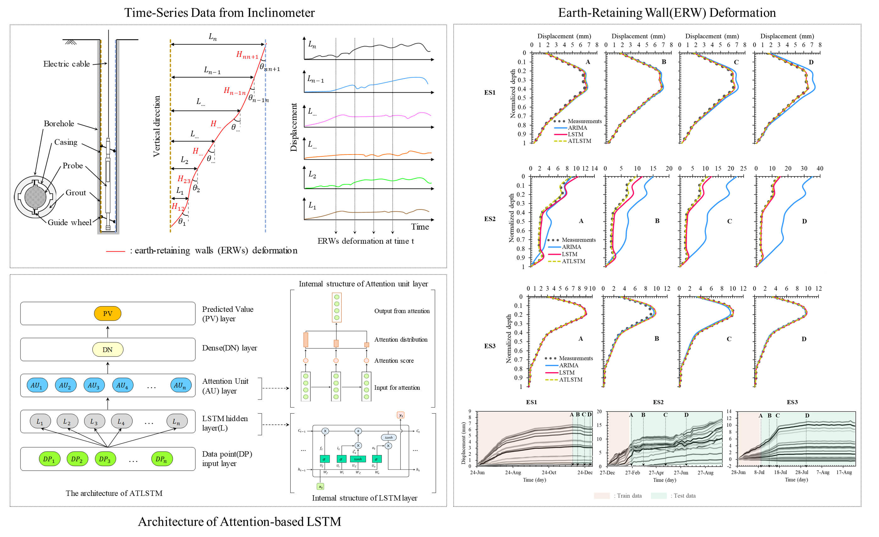
The Long Short-Term Memory (LSTM) model is a type of neural network designed to address the long-term dependency problem commonly encountered in traditional Recurrent Neural Networks (RNNs) [43]. The internal structure of an LSTM cell, as depicted in Fig. 1, represents the hidden layer at time t. Here, xt denotes the input vector at time step t. The terms ht−1 and ht represent the hidden state vectors at time steps t−1 and t, respectively, managing short-term memory information. Similarly, Ct−1 and Ct are the cell state vectors at time steps t−1 and t, which handle long-term memory information. Within the LSTM cell, various mechanisms process the input vector and hidden state vector. These operations are defined by Eqs. (4) to (9).

ft=σ(Ufht−1+buf+Wfht+bwf)(4)

it=σ(Uiht−1+bui+Wiht+bwi)(5)

ot=σ(Uoht−1+buo+Woht+bwo)(6)

C~t=tanh(UC~ht−1+buC~+WC~ht+bwC~)(7)

Ct=(ft⊗Ct−1)⊕(it⊗C~t)(8)

ht=ot⊗tanh(Ct)(9)

time step t−1, the hidden state vector ht−1 is propagated through the forget gate (ft), input/update gate (it), output gate (ot), and cell input (C~t) by multiplying respective tensors Uf, Ui, Uo, and UC~, before transmission. Similarly, the input vector xt is propagated to each gate by multiplying tensors Wf, Wi, Wo, and WC~. The bias vectors buf, bui, buo, buC~, bwf, bwi, bwo, and bwC~ are also applied. The sigmoid σ and tanh activation functions are utilized. The symbols ⊕ and ⊗ denote element-wise vector addition and multiplication, respectively. The forget gate vector, activated by the sigmoid function, takes values between 0 and 1. Therefore, if the previous cell state vector Ct−1 is deemed necessary to remember, it learns to approach 1. Conversely, if it is deemed unnecessary, it learns to approach 0. The long-term memory cell state vector Ct is computed by element-wise multiplication of the previous cell state vector Ct−1 with the forget gate vector, combined element-wise with the product of the input gate vector and the cell input vector. The resultant hidden state vector ht, which is transmitted vertically and horizontally, is derived by applying the tanh activation function to the cell state vector and then element-wise multiplying by the output gate vector.

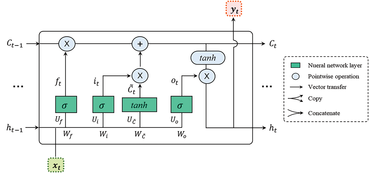
Figure 1: Basic structure of LSTM with forget gate, input gate, and output gate

2.3 Attention Mechanism

Attention mechanisms in neural networks operate as a weighted average of values, where the weighting function is learned rather than predefined. This method functions analogously to a form of memory that accumulates by focusing on various inputs over time. The primary objective of attention mechanisms is to enhance feature extraction from the input, enabling the model to accurately represent complex dynamics present in the data. A crucial aspect of attention is its ability to focus selectively on particular features, effectively reducing bottlenecks within the model. Additionally, attention mechanisms often address the issue of vanishing gradients by establishing direct connections between the states of the encoder and decoder, as illustrated in Fig. 2. This figure depicts the attention mechanism’s architecture, including the inputs, attention scores and their distribution, and the outputs.

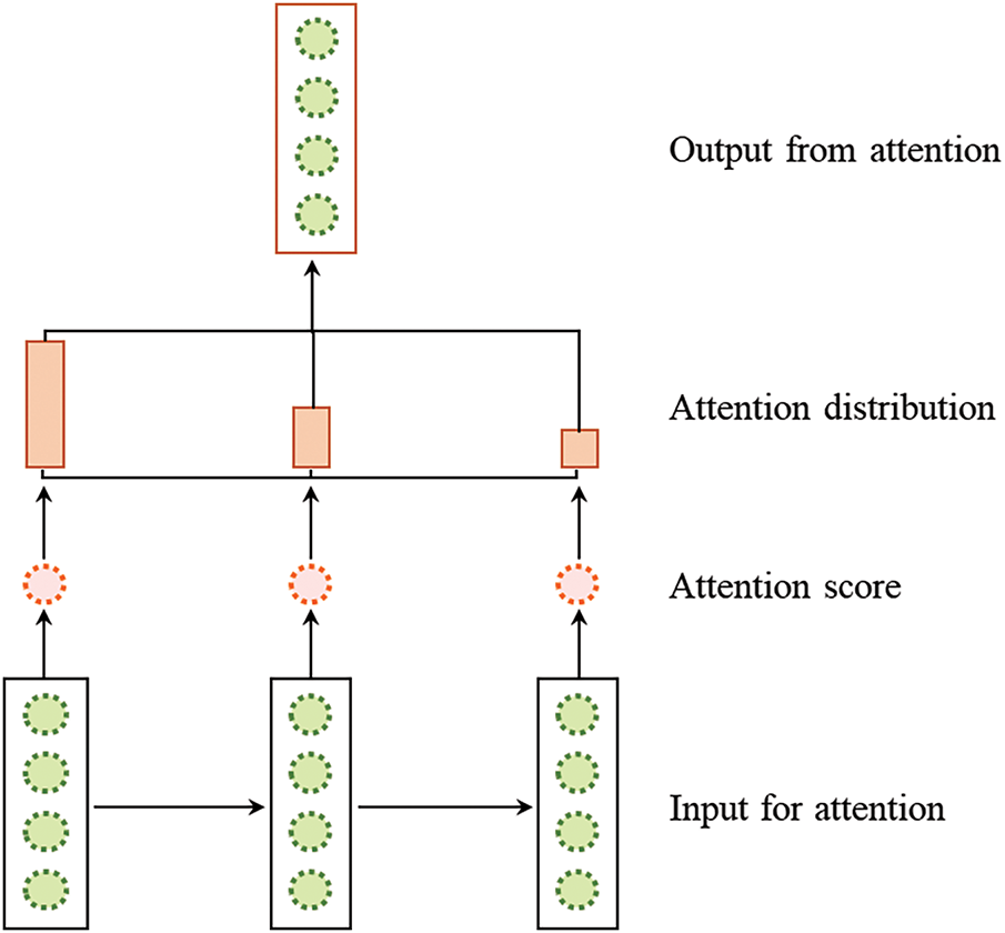
Figure 2: Schematic diagram of the attention mechanism

Developed by Bahdanau et al. [44], the attention mechanism involves several key processes: calculating attention scores, assigning preferential weights, and distributing context vectors. These processes are executed in a defined sequence. Initially, the attention score is calculated based on how well parts of the input sequence align with the current output at a specific position t. This calculation, denoted as et,i, considers both the encoded hidden states hi and the previous decoder output St−1. The function a(.), potentially implemented via a feedforward neural network, computes this score as shown in Eq. (10).

Following the computation of the attention score, the softmax operator is applied to determine the weights et,i, as formulated in Eq. (11). Subsequently, a unique context vector ct is derived by summating the product of these weights with the encoder hidden states. This context vector is then fed into the decoder at each timestep, as expressed in Eq. (12).

et,i=a(st−1,hi)(10)

αt,i=softmax(et,i)(11)

ct=∑i=1Tαt,ihi(12)

Here, ct represents the context vector at decoder timestep t, and it captures a weighted sum of all encoder hidden states hi, where the weights αt,i reflect the relevance of each encoder state to the current decoding step. This vector essentially summarizes the most relevant information from the entire input sequence to help the decoder generate the appropriate output at time t. Notably, the attention mechanism enhances computational efficiency by reducing memory requirements and minimizing the impact of irrelevant or noisy data. This allows for more precise and effective modeling, particularly in tasks involving complex input-output relationships.

2.4 Attention-Based LSTM

As previously noted, while LSTM networks have addressed some weaknesses inherent to RNNs, they are not without limitations. For instance, LSTM networks can manage sequences up to approximately 20 steps effectively but struggle with longer sequences [45]. Moreover, traditional LSTMs often fall short in delivering realistic and accurate forecasts. To overcome these challenges, we have integrated an attention mechanism with the LSTM network, forming an enhanced model designated as Attention-based LSTM (ATLSTM). This integration aims to correct the deficiencies of conventional RNNs and optimize the LSTM architecture for better predictive accuracy. The structure of the ATLSTM, including the internal configuration of the attention unit and the LSTM layers, is depicted in Fig. 3. The architecture of the proposed ATLSTM network comprises five sequential layers: an input layer, an LSTM layer, an attention layer, a dense layer, and an output layer. The input layer initially receives data points that feed into the model. Subsequent processing occurs in the LSTM layer, where the long short-term memory unit transforms inputs into refined features. The attention layer then calculates a weight vector that emphasizes more significant weights within the hidden state information, affecting all subsequent hidden states. The dense layer, known for its fully-connected nature, links every neuron in one layer to every neuron in the next. Finally, the output layer utilizes feature vectors for analyzing and predicting time-series data.

Figure 3: Architecture of attention-based LSTM (ATLSTM) showing the internal structure of the attention unit and LSTM layer

Incorporating the attention mechanism within the LSTM framework addresses the challenge of managing long-sequence data, providing a dynamic solution that enhances data interpretability. This approach allows for a more nuanced assignment of weights to critical parts of the input data, thus facilitating more precise and accurate forecasts, particularly in production environments. By merging the LSTM with the attention mechanism, the model not only retains its efficacy with time-series data but also significantly improves in forecasting accuracy, even in the presence of noisy data. This study contributes substantially to the field by exploring the integration of the attention mechanism into the LSTM network, including strategic considerations such as the placement of the attention layer—whether before the dense layer or after a dropout layer—and the optimal number of attention layers.

3  Methodology

3.1 Data Description and Preprocessing

In general, the deformation of ERWs due to excavation work is measured using a guide wheel fixed series inclinometer. The length of the inclinometer depends on the depth of excavation, and the spacing of the series inclinometers is 0.5 or 1 m. The bottom of the inclinometer is fixed to the immobile layer and the horizontal displacement of the bottom is set to zero to calculate the relative displacement along the wall. The displacement is then measured at each point at regular time intervals. The procedure for measuring wall deformation using the inclinometer shown in Fig. 4 is as follows.

L1=H12sinθ1(13)

L2=H23sinθ2+L1(14)

Ln=Hnn+1sinθn+∑1n−1Li(15)

where Ln represents the horizontal displacement of the n th monitoring point; Hnn+1 represents the distance between the n th and (n + 1) th monitoring points (generally a fixed value of 0.5 m). θn represents the inclination angle of the connection line between n th and (n − 1) th monitoring points.

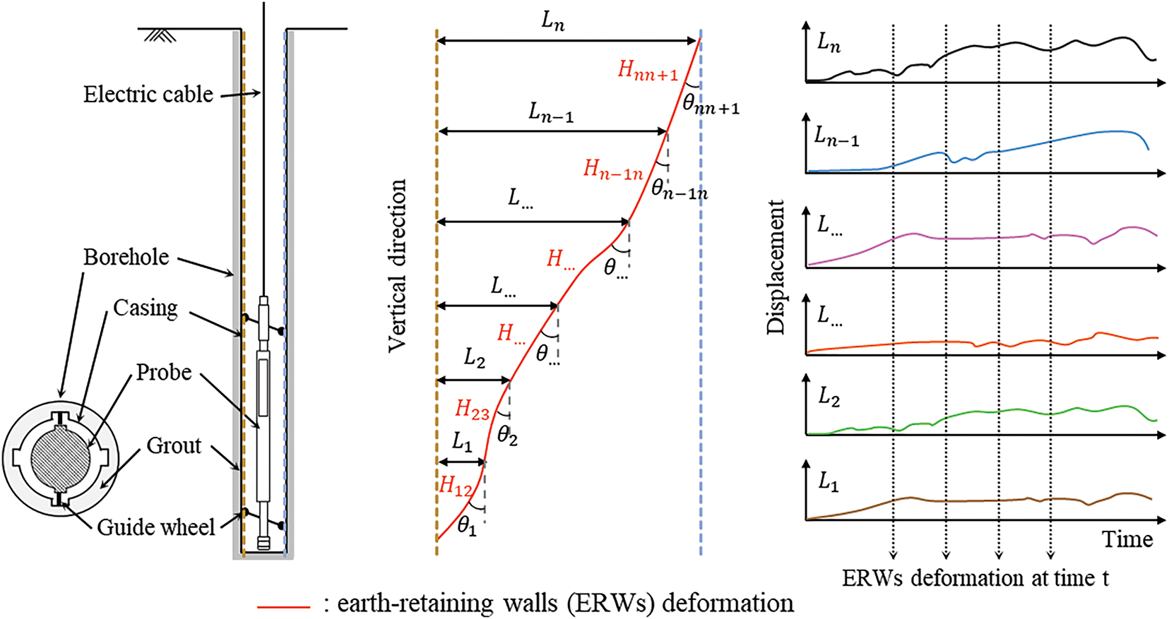
Figure 4: Measuring ERWs displacement using inclinometer probe (modified from Dunnicliff [46])

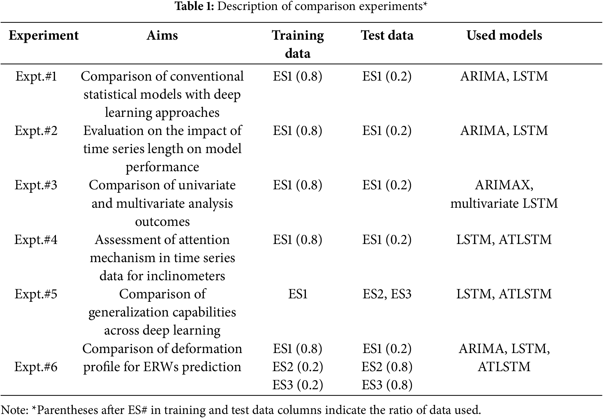
In this study, we utilized time series data from inclinometers across three distinct excavation sites, as represented in Fig. 5. The data encompass entire representative profiles from each site, with each time series varying in terms of excavation duration, depth, and the number of data points. Patterns of time series data from inclinometers also varied by depth. Using time series data from these three sites (labeled ES1, ES2, and ES3), we conducted experiments under various conditions as outlined in Table 1, performing a total of six experiments. This approach allowed us to analyze the characteristics of ERW deformations due to excavation and to meticulously compare traditional statistical-based models with deep learning models, examining the advantages and disadvantages of each method.

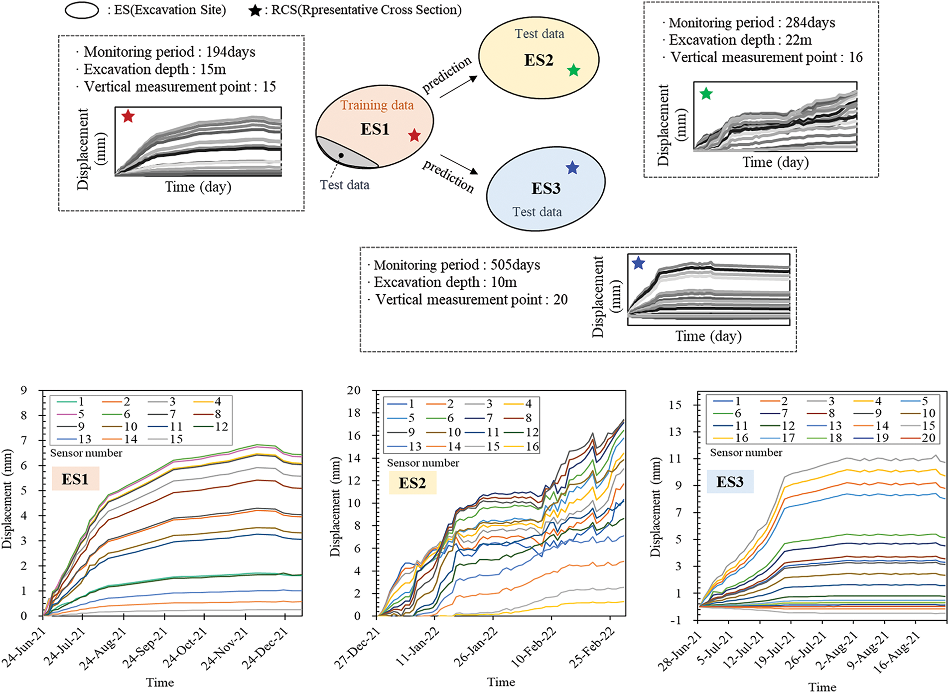
Figure 5: Conceptual illustration of time series data-collection from an inclinometer at excavation sites

To further describe the three monitoring sites, ES1 corresponds to a relatively deep excavation site with a final depth of approximately 15 m. The stratigraphy at ES1 consists of artificial fill, clayey sedimentary deposits, and highly weathered granite. The site features soft-to-medium stiff clay layers in the upper portion and dense silty sand at deeper depths. Groundwater levels ranged from 4 to 6 m depending on the borehole. ES2 represents the deepest excavation among the three, reaching a maximum depth of 22 m. This site was excavated in two stages and mainly comprises weathered granite and dense silty sand layers, with the groundwater table located near 6 m. ES3 involves a medium-depth excavation of about 10 m. The ground conditions consist primarily of filled soils overlying weathered silty sand with medium to high relative density. The groundwater level was observed at a depth of around 5 to 6 m. Although these geotechnical conditions were not directly used as input variables in the predictive models, they help explain the deformation behavior observed in the measured time series data. The purpose of excluding these parameters was to evaluate the predictive capability of the time series-based model using only inclinometer data collected in real time during excavation, thereby simplifying the model and reducing interpretive uncertainty.

Data preprocessing was the initial step in analyzing the time series data for inclinometers, as illustrated in Fig. 6. Given the variations in excavation duration, data collection intervals, and lengths of time series data at each site, normalization was essential. We normalized the maximum excavation depth of each profile as depicted in Fig. 7. In multivariate analysis, measurements from different depths were utilized as exogenous variables or features, enabling the selection of desired variables. Excavation depths were scaled to a range of 0 to 1, with normalized values denoted as hN. Inclinometer measurements were normalized to a range of 0 to 1 based on minimum and maximum values, as indicated in Eq. (16).

yi=xi−min(xi)max(xi)−min(xi)(16)

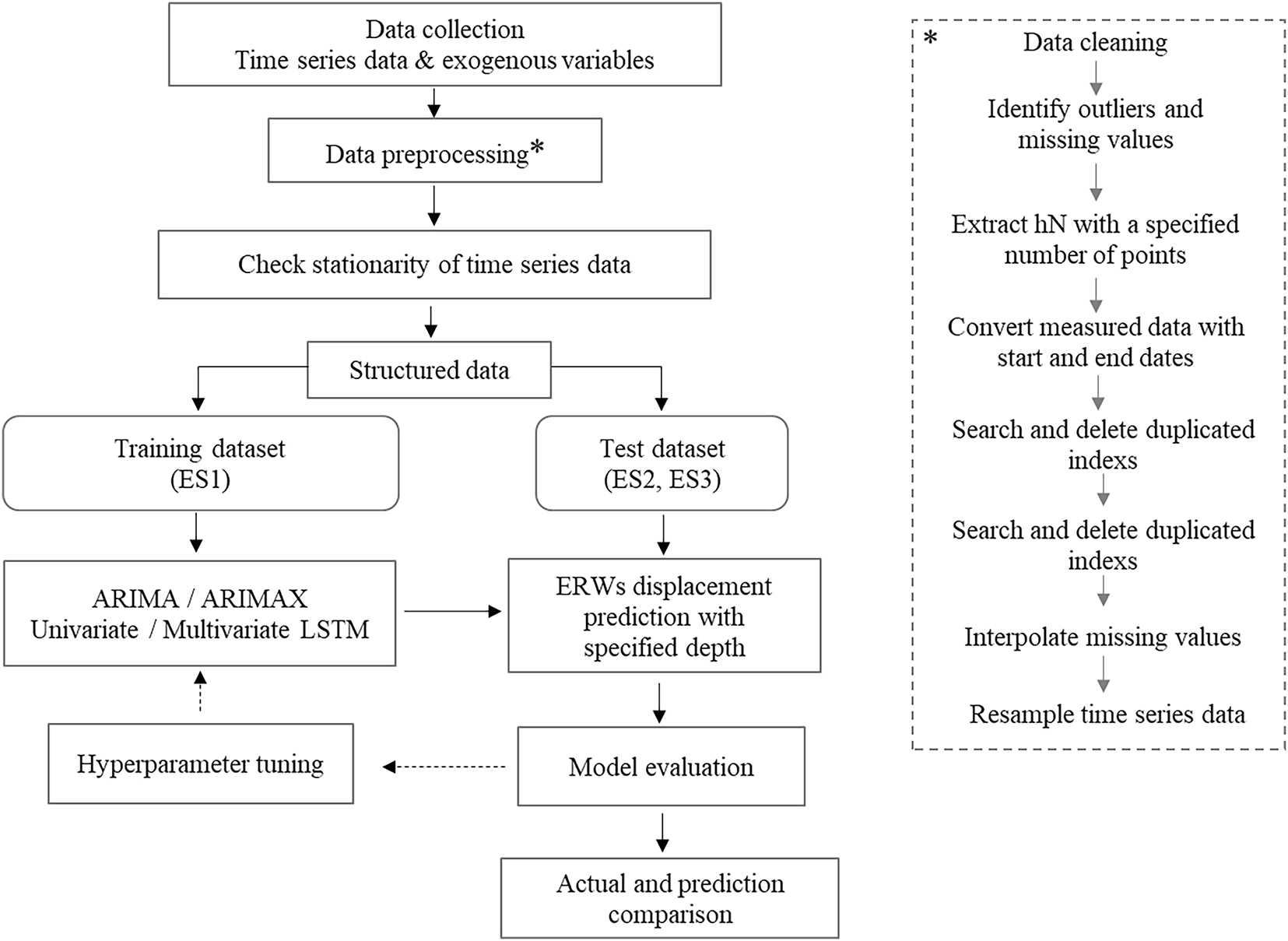
Figure 6: Data preprocessing and analysis procedures for inclinometer time series

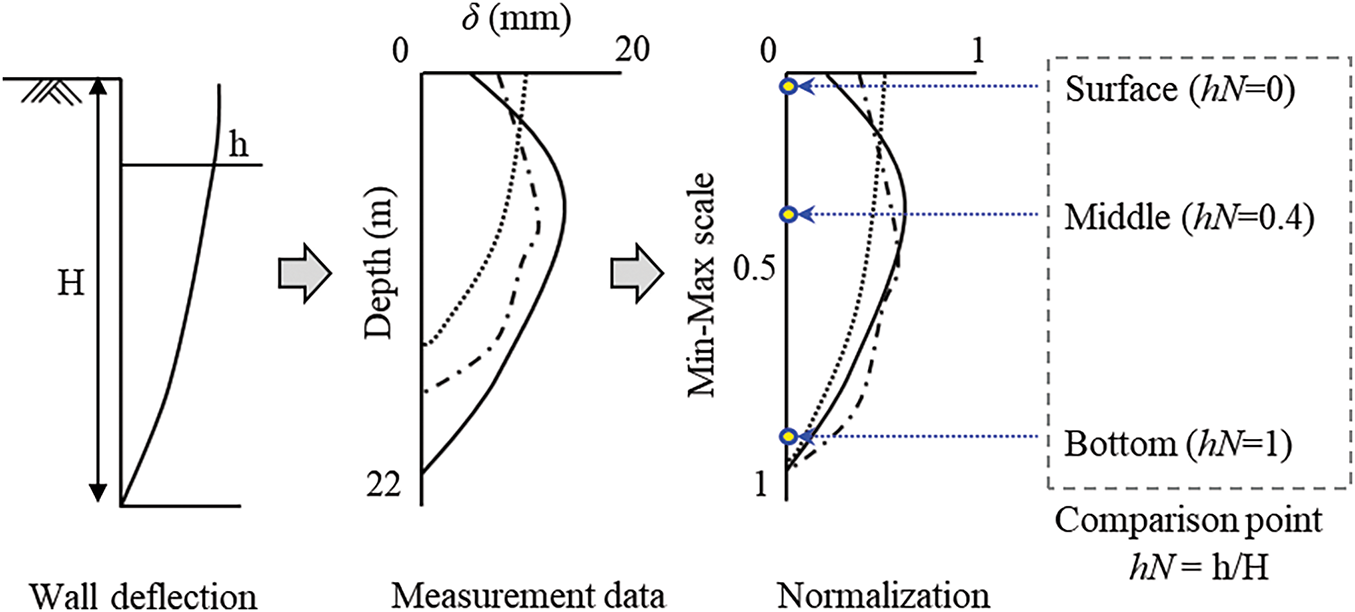
Figure 7: Schematic of normalization for inclinometer measurements

To assess the impact of predictive models based on the degree of displacement across various depths of ERWs, we established analysis points at the surface, middle, and bottom of the wall, corresponding to hN values of 0, 0.4, and 1, respectively.

Following the spatial scaling of inclinometer measurements, preprocessing was performed for time intervals (time steps). Initial data preprocessing involved identifying overlapping dates between the start and end of excavation, selecting one occurrence from any duplicates, and generating a dataset indexed by time. The sequence length was reconstructed based on day-interval data covering the entire period of excavation. Missing data due to measurement intervals were addressed through linear interpolation, ensuring that the overall structure of the time series remained unchanged. The sequence length for analyses, such as in Expt. 3, was adjusted to day-based time series data, and up-sampling techniques were applied to increase the resolution of time steps, allowing us to closely extract time intervals. Thus, for instance, ES1’s 195 steps of day-based sequence data were up-scaled to 300, 500, and 1000 steps. It is noted that when sequence lengths exceed 1000 steps, LSTM models may experience performance degradation; therefore, we capped the maximum at 1000 steps for performance comparison [47].

3.2 Input Variables

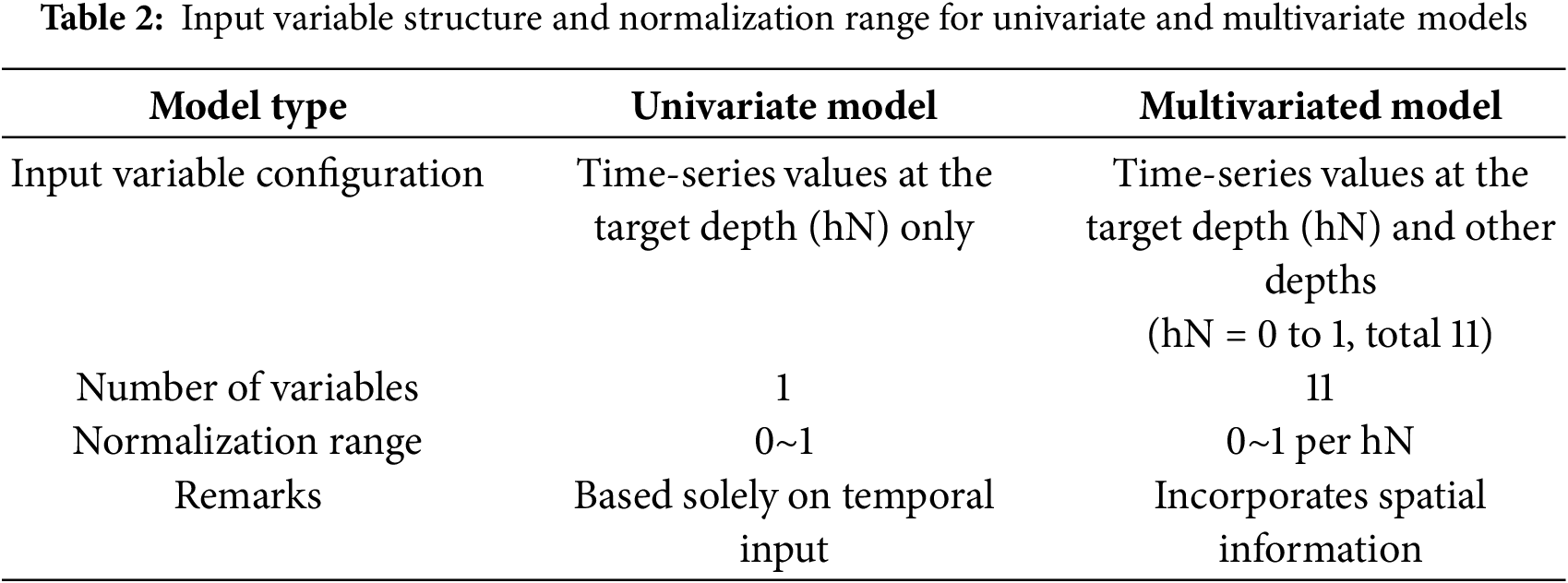
Previous studies [34–36] employed various types of variables, including ground information and numerical analysis results, for predicting the deformation of ERWs. This research, however, focuses primarily on the time series analysis of geotechnical measurement data, deliberately omitting ground investigation and structural data as input variables to reduce uncertainty in model interpretation. Only inclinometer measurements at specific depths were used, with measurements at the target depth labeled for univariate models, and measurements at other depths treated as exogenous variables or features for multivariate models. Fig. 8 displays the values used in both univariate and multivariate predictive models for input variables (hN 0 to 10). Consequently, predictive models were developed for each normalized depth value, hN, and used to forecast deformations across the entire depth of ERWs. To clarify the structure of the input variables and normalization strategy for both model types, Table 2 presents a detailed summary of their configurations. The univariate model uses only the time-series data at the target depth (e.g., hN = 0.5), whereas the multivariate model incorporates time-series data from all normalized depths ranging from hN = 0 to hN = 1 (in total, 11 depth levels). In both cases, data normalization was performed over the range 0 to 1, but for multivariate inputs, normalization was applied individually per depth level to preserve relative variation across depths. The multivariate model structure thus enables the model to learn spatial deformation patterns by utilizing adjacent inclinometer measurements, while the univariate model relies exclusively on temporal patterns at a single depth.

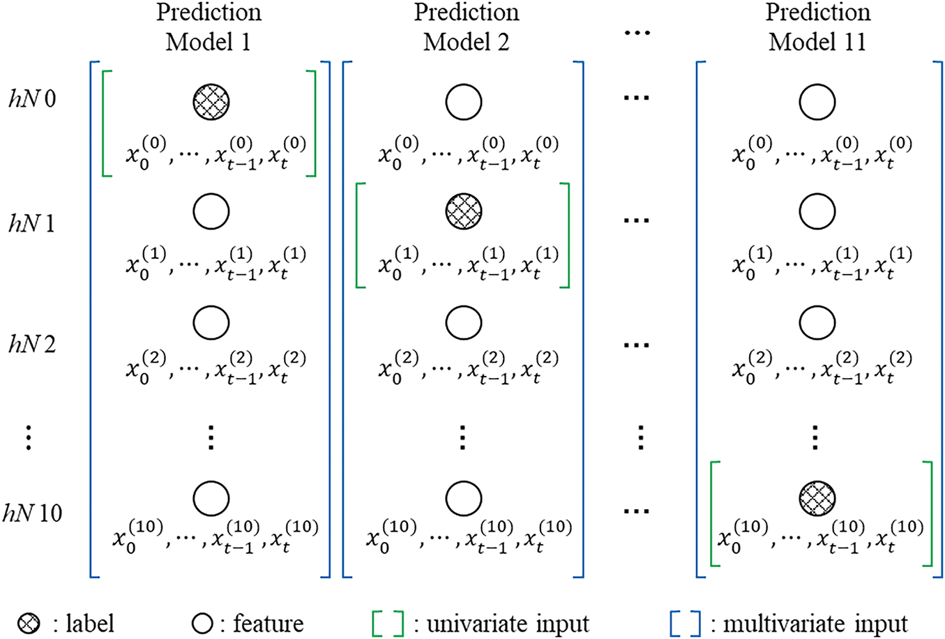
Figure 8: Overview of input variables for univariate and multivariate prediction models

3.3 Model Structures and Hyperparameter Selection

To establish an effective prediction framework for time series deformation of earth-retaining walls, two deep learning architectures were adopted and optimized: a conventional LSTM model and an attention-based LSTM (ATLSTM) model. Each model’s architecture was carefully designed to capture both short- and long-term temporal dependencies within the inclinometer measurement data.

The LSTM model consists of a single long short-term memory (LSTM) layer that processes sequential input data over a predefined window size. This layer extracts temporal features from the input sequence and passes them to a dropout layer, which helps prevent overfitting by randomly deactivating a fraction of the units during training. The final prediction is obtained through a fully connected dense layer that outputs a single displacement value. In contrast, the attention-based LSTM (ATLSTM) model extends the structure of the basic LSTM by incorporating multiple stacked LSTM layers, each configured to return sequences. This is essential for enabling the attention mechanism to operate over the entire sequence of hidden states. After the final LSTM layer, an attention mechanism is applied to compute the relative importance of each time step in the input sequence. Attention weights are assigned through a softmax function, allowing the model to focus more heavily on time steps that are more informative for the prediction task. These weighted features are then aggregated through a weighted sum, followed by a dense layer that produces the final output.

To determine optimal model configurations, a comprehensive hyperparameter sensitivity analysis was conducted. Four key parameters were explored: the number of LSTM layers (ranging from 1 to 5), the number of hidden units per layer (5 to 50), batch size (16, 32, 64, 128), and learning rate (from 1e−4 to 1e−2). Fig. 9 presents two heatmaps visualizing the impact of these parameters on model performance, measured by mean absolute error (MAE) on the validation set. The results showed that for the ATLSTM model, the best performance was achieved using two LSTM layers with 10 hidden units each. Increasing the number of layers or units beyond this configuration did not yield further improvements and, in some cases, degraded performance due to overfitting. Additionally, models trained with smaller batch sizes (16 or 32) and lower learning rates (1e−4 to 1e−3) exhibited more stable convergence and lower validation errors. In contrast, large batch sizes combined with high learning rates resulted in unstable training behavior and increased error. Based on this analysis, the final configuration selected for the ATLSTM model consisted of two LSTM layers, each with 10 hidden units, a batch size of 32, and a learning rate of 0.001. These settings were used consistently in subsequent experiments to ensure both high accuracy and stable generalization performance.

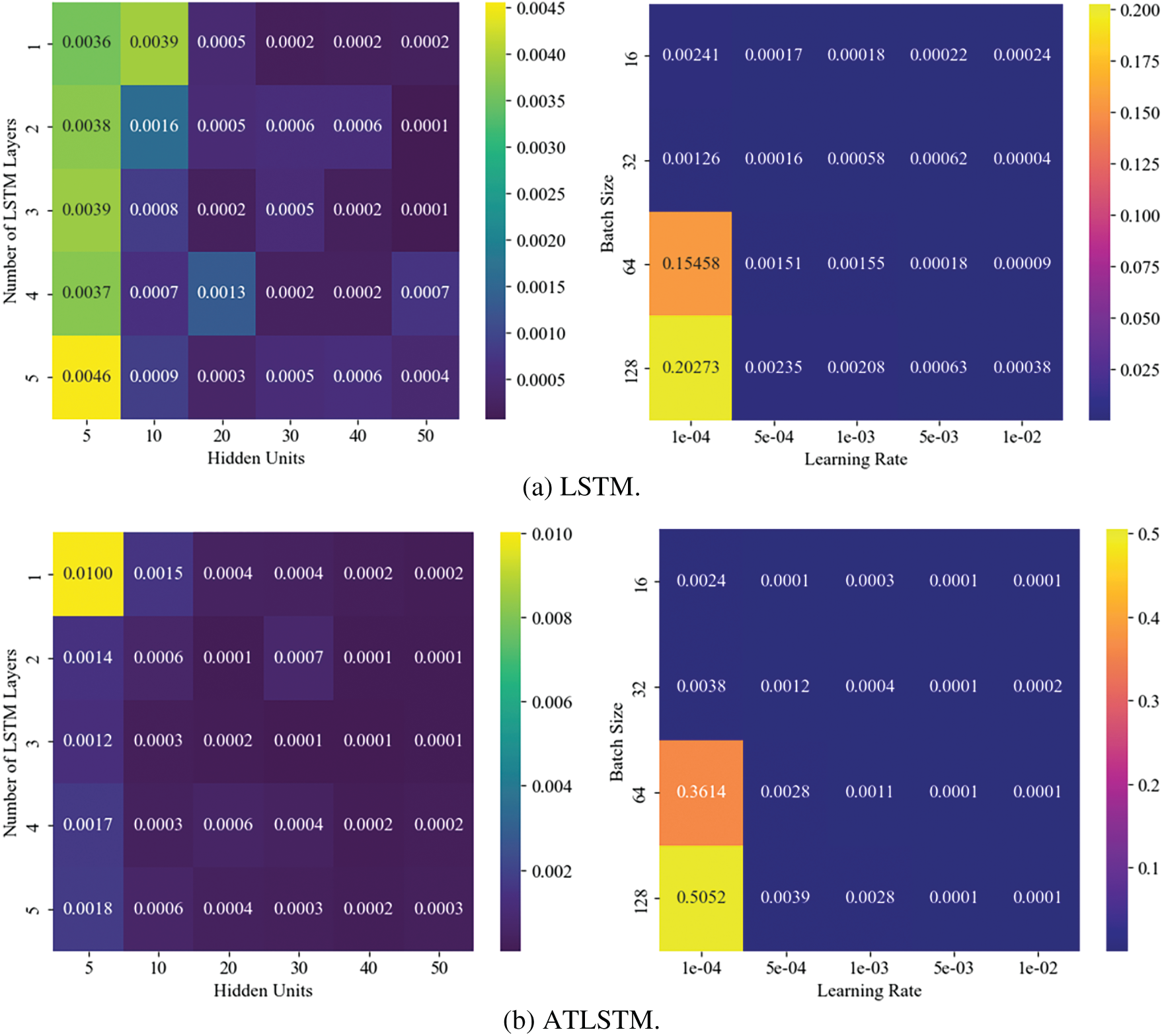
Figure 9: Hyperparameter sensitivity analysis of LSTM and ATLSTM model

Based on this analysis, the final configuration selected for the ATLSTM model consisted of two LSTM layers, each with 10 hidden units, a batch size of 32, and a learning rate of 0.001. These settings were consistently applied in subsequent experiments to ensure robust performance and generalization. To further evaluate the real-time applicability of the models, we measured their computational efficiency in terms of training time and inference latency. On a system equipped with an Intel Core i9-12900K CPU (3.2 GHz), 64 GB RAM, and an NVIDIA RTX 3090 GPU, the training time for the conventional LSTM model was approximately 2.8 s, with an inference time per sample of 0.003 s. The ATLSTM model required a slightly longer training time of 3.1 s and an inference time of 0.01 s. These results indicate that both models, especially given their rapid inference speed, are computationally lightweight and suitable for real-time deformation monitoring applications in practice.

3.4 Model Training and Evaluation

Following the procedures described, raw data can be preprocessed to prepare time series data with sampling frequency normalized to daily intervals. When applying time series data to deep learning models, it is necessary to define the window size (W), which sets the range of past information the model considers. In this study, the quantity of past information the LSTM model can recall was determined by setting W between 5 and 25 through iterative experiments, with optimal performance observed at window sizes of 5 and 10. For the model training, 20% of the entire dataset was designated as the test data set, while the remainder was used as the training data set. For instance, for site ES1, the period from 24 June 2021, to 26 November 2021, served as the training data, whereas the period from 27 November 2021, to 4 January 2022, constituted the test data. To prevent overfitting, 20% of the training data was utilized as validation data.

To verify the convergence and training stability of the proposed models, training and validation loss curves were plotted for both the LSTM and ATLSTM models, as shown in Fig. 10. The training loss for both models decreased rapidly within the first few epochs and continued to converge stably thereafter. The validation loss also closely followed the training loss, demonstrating that no significant overfitting occurred. In particular, the LSTM model exhibited lower overall loss values with faster convergence, whereas the ATLSTM model showed slightly higher validation loss but maintained consistent stability throughout training. These results support that both models were well-regularized and effectively trained, ensuring reliability in subsequent predictive performance.

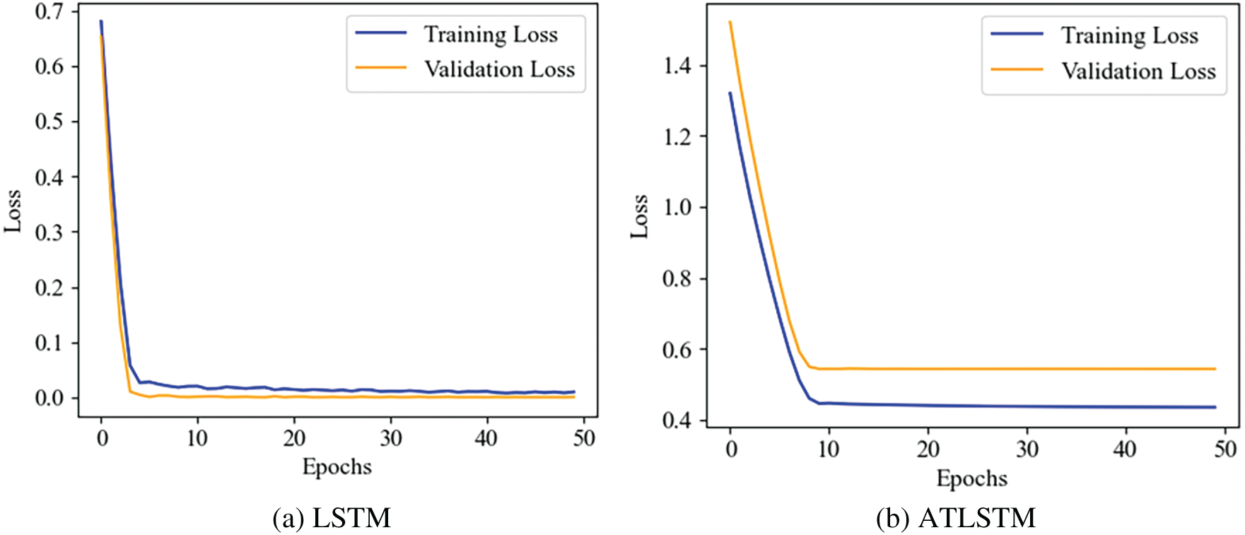
Figure 10: Training and validation loss curves for LSTM and ATLSTM

The final prediction results were assessed using three common performance metrics: Root Mean Square Error (RMSE), Mean Absolute Error (MAE), and Mean Absolute Percentage Error (MAPE).

RMSE=1n∑i=1n(y^i−yi)2(17)

MAE=1n∑i=1n|y^i−yi|(18)

MAPE=∑i=1n|y^i−yiyi|100% n(19)

Here, yi represents the actual measured values, and y^i denotes the values predicted by the model. MAE, the average of absolute errors, provides an intuitive assessment of error but lacks sensitivity to the magnitude of errors. RMSE reduces the distortion of under-predicted items, with smaller values indicating higher precision. MAPE, which represents MAE as a ratio, facilitates an intuitive assessment of errors and is useful for comparing predictive performance across models.

4  Results and Discussion

4.1 Prediction Results by ARIMA and LSTM

In this study, time series analysis of inclinometer data at various depths was performed using both ARIMA and univariate LSTM models. Prior to using the ARIMA model, it was necessary to confirm the stationarity of the data. As indicated by Fig. 11, the autocorrelation coefficient (ACF) exceeded the acceptable limits starting at lag 13, showing a gradual decline with increasing lags, suggesting non-stationary data. The partial autocorrelation function (PACF) converged to zero after the third lag, and the differencing order d was estimated at 2, after which the Dickey-Fuller test yielded a p-value less than 0.05, confirming that the data could be transformed to stationarity. The parameters p and q were iteratively tested to optimize the Akaike Information Criterion (AIC), ultimately selecting 4, 2, and 3 for p, d and q, respectively.

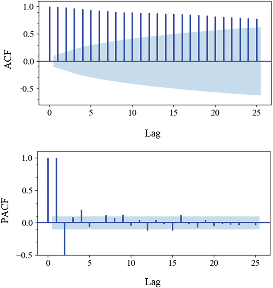
Figure 11: Correlation analysis utilizing autocorrelation function (ACF) and partial autocorrelation function (PACF) for time series data from ES1

Fig. 12 presents the prediction results for the test dataset using both the ARIMA and LSTM models. The MAPE was 5.6042% for ARIMA and 1.5259% for LSTM, indicating superior overall performance of the LSTM model. The LSTM also showed lower RMSE and MAE, indicating smaller prediction errors. However, ARIMA demonstrated advantages in short-term predictions. Fig. 13 shows the measured and predicted values at the depth with maximum displacement. For the initial 4 days of the test period starting November 27, the ARIMA model performed better, but over the entire 36-day forecast period, LSTM predicted the actual measurements with a similar pattern and exhibited superior long-term prediction performance as reflected by the MAPE metric. The ARIMA model proved effective for short-term predictions up to about 3–4 days but was less accurate over longer durations. ARIMA assumes that past patterns, which are stationary, will repeat in the future. In contrast, inclinometer data for ERWs displacement, which are inherently non-stationary, show that recent measurements correlate more significantly with current values. Therefore, ARIMA requires transformation through differencing to be effective for short-term predictions, and care must be taken when sudden changes in measurements occur, as this can lead to significant errors. LSTM models, in general, exhibit superior performance in both short- and long-term predictions and are particularly advantageous for non-stationary data like earth-retaining wall displacement.

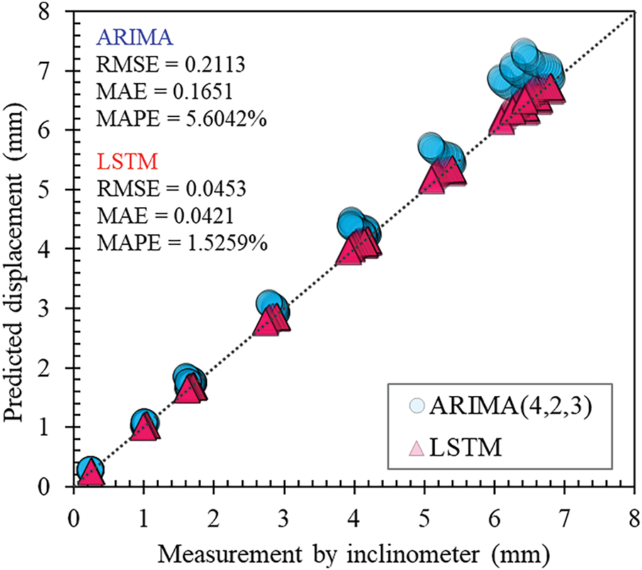
Figure 12: Comparative analysis of actual vs. predicted values for ARIMA and LSTM models

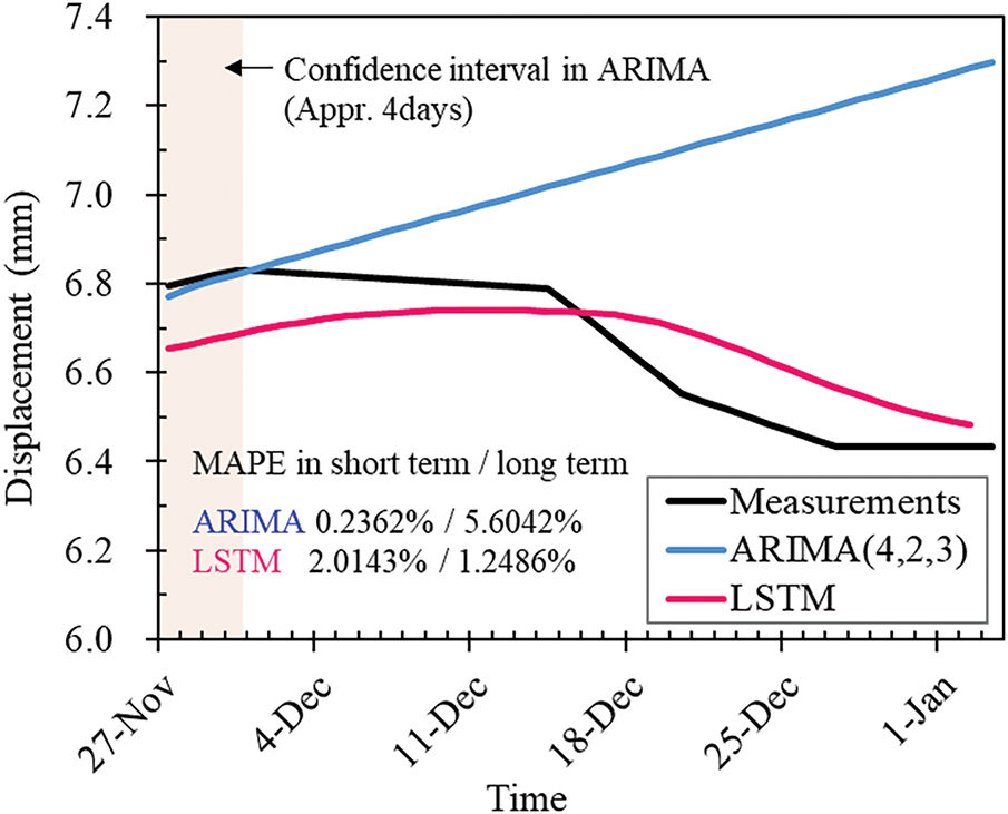
Figure 13: Prediction results for ARIMA and LSTM at hN = 0.4

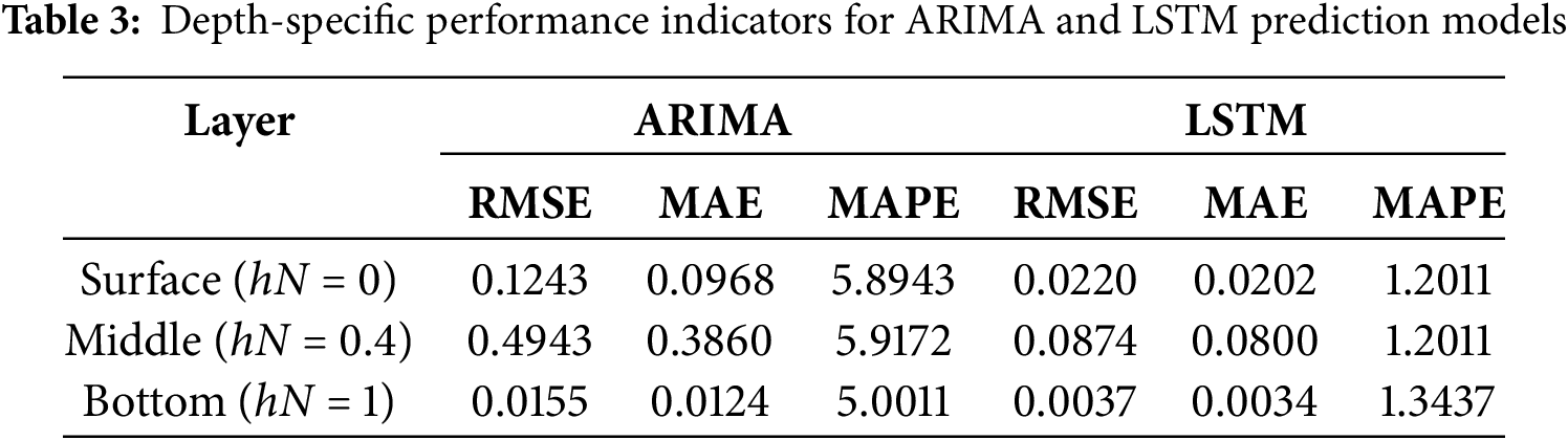
Fig. 14 displays the prediction results for various depths, with performance metrics detailed in Table 3. Table 3 illustrates the prediction results at comparative points on the ERW as shown in Fig. 7, allowing for an assessment of differences in model predictions by depth. Overall, LSTM exhibited lower errors across the entire wall. Individually, the ARIMA model showed lower errors at the bottom, likely due to smaller overall displacement changes, thus less non-stationarity in the time series data relative to the surface and middle sections. The lower performance of LSTM at the bottom might be attributed to relatively smaller displacement changes at greater depths, leading to less distinct time series patterns. In summary, while ARIMA is highly sensitive to depth-specific data characteristics, LSTM consistently predicts actual measurement patterns more accurately across various depths.

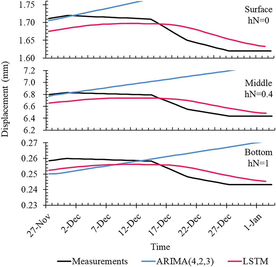
Figure 14: Depth-specific prediction results for ARIMA and LSTM models

4.2 Prediction Results Based on Time Series Length

In this study, the impact of sequence length (L) on the performance of time series prediction models was examined. Sequence length signifies the amount of information a time series prediction model can learn, thus influencing its performance. By up-sampling day-based data to sequence lengths of 300, 500, and 1000, the resolution of time series data was adjusted to explore its effect on prediction models. With the increase in L values, parameters for the ARIMA model were reselected for optimal performance, while the window size for LSTM was fixed at 30. Fig. 15 illustrates the variation in MAPE with increasing L values, showing that error decreases and overall performance improves for both prediction models. LSTM is effective for both short- and long-term prediction performance as sequence length increases, while ARIMA does not show significant improvement.

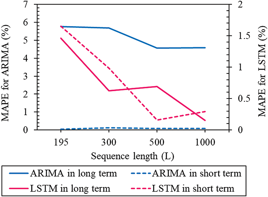
Figure 15: MAPE results by available sequence length

Fig. 16 displays the actual and predicted values for the test data. For ARIMA, while there is a slight improvement in prediction performance with increased L values, long-term prediction capabilities did not show significant enhancement. Additionally, it was observed that short-term prediction performance within 5 days deteriorated. Conversely, LSTM exhibited improvements in both short- and long-term prediction performance as L increased. Short-term prediction performance showed improvements up to L of 500, while a substantial enhancement in long-term prediction performance compared to short-term predictions was evident when L reached 1000. Thus, for LSTM, adjusting the resolution of time series data through data augmentation appears to enhance both short- and long-term prediction performance. This suggests that the finer representation of data patterns due to increased sequence length effectively boosts prediction capabilities. For ARIMA, maintaining the original time intervals of the time series data when building the prediction model is crucial, and using the original data with parameter tuning, rather than up-sampling, is deemed more appropriate. This approach likely retains the integrity of the original temporal patterns, which is essential for the effective application of ARIMA models in time series prediction.

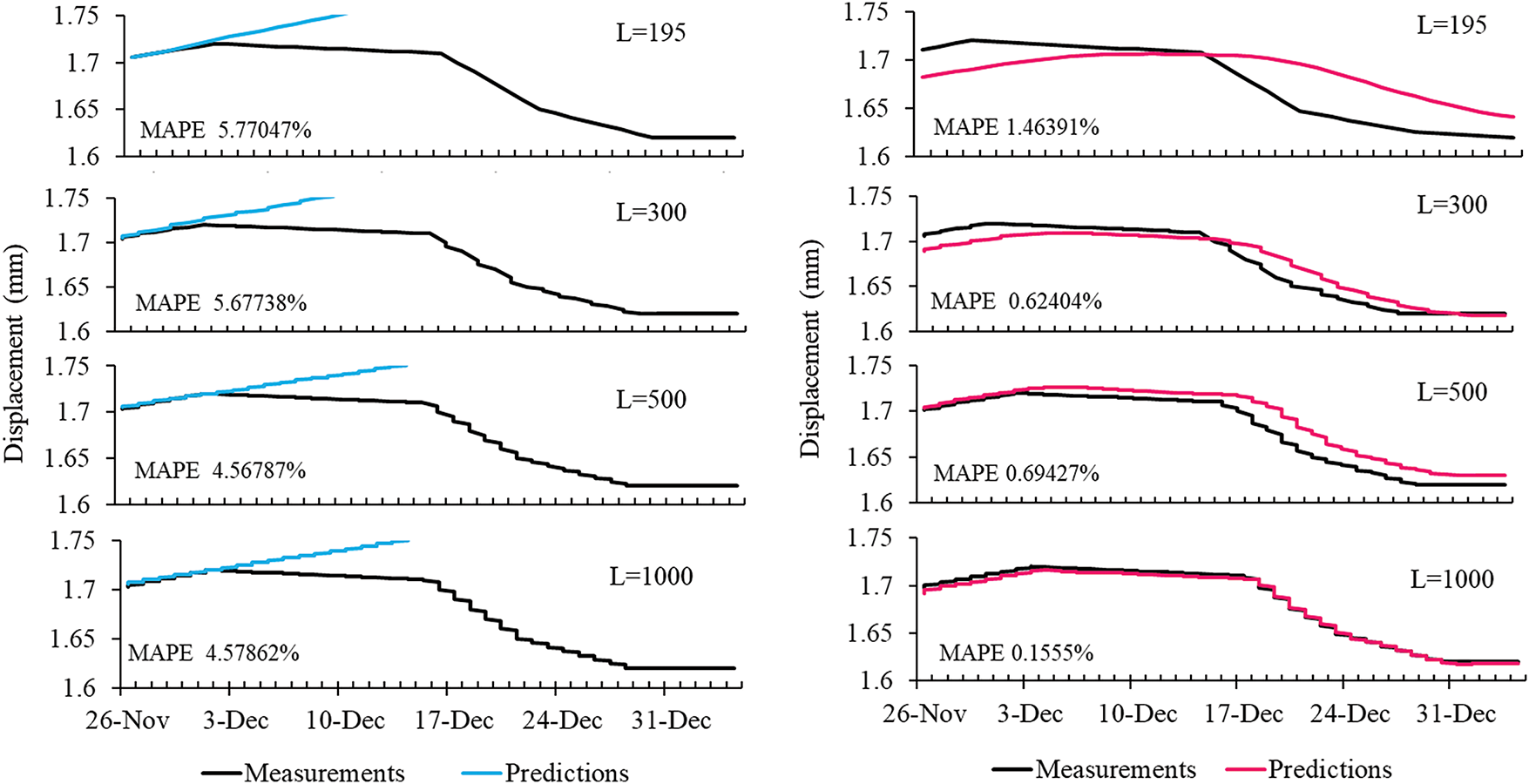
Figure 16: Comparative analysis of prediction results by sequence length

Among various resampling techniques, up-sampling is known to be the most effective in enhancing prediction performance [48]. In our study, up-sampling was applied to adjust sequence lengths, which maintains the structural integrity of the data while potentially improving prediction performance for the specific data used. However, enhancing generalization performance across diverse data characteristics using this method alone might be challenging. To improve generalization, incorporating a variety of field measurement data or introducing noise to transform the structural properties of time series data for use as training material may be more effective.

4.3 Prediction Results by ARIMAX and Multivariate LSTM

In this study, we employed two models capable of multivariate analysis. These models used inclinometer measurements from various depths as exogenous variables or features to compare prediction performance in a multivariate context. Fig. 17 displays the measured and predicted values by comparison depths, and Table 4 presents the performance indicators of the prediction models. Significant differences were observed between the univariate ARIMA and the multivariate ARIMAX. It was noted that, excluding hN = 1, the ARIMAX showed considerable improvement in prediction results. However, it appears that the ARIMA was excessively influenced by the measurements from other depths used as exogenous variables, suggesting that the ARIMAX did not genuinely learn the dynamic characteristics of the time series but rather followed the displacement patterns of surrounding depths as exogenous variables. This implies an excessive dependency on future changes in the exogenous variables, making the model overly sensitive and potentially less effective in real-world applications.

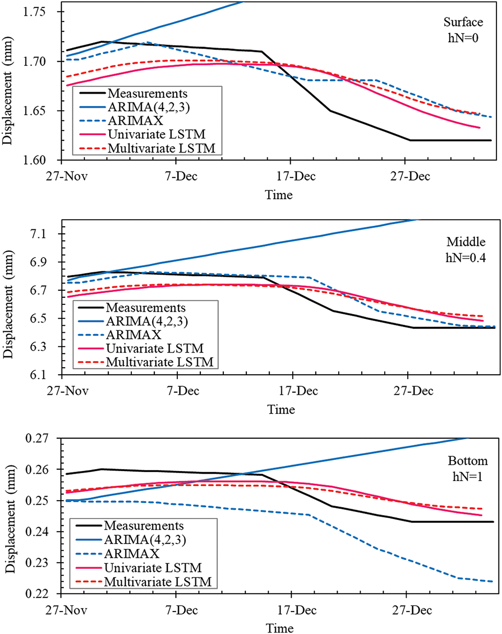
Figure 17: Comparison of prediction outcomes for ARIMAX and multivariate LSTM models

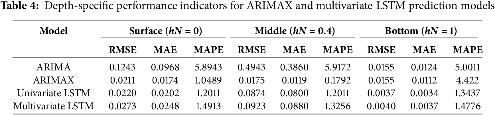
For the LSTM, there was not a significant difference between univariate and multivariate results, indicating that the displacement values across various depths generally followed similar patterns, thus not significantly influencing predictions. Typically, the use of multiple input variables in a multivariate LSTM leads to increased complexity and improved predictive power. However, in cases like inclinometer displacement data, where the temporal changes are minimal and the patterns relatively straightforward, depth-specific measurements do not provide additional predictive value. Therefore, employing a univariate LSTM model to aggregate predictions across different depths for predicting overall ERW deformations is deemed effective.

4.4 Comparison of Prediction Results between LSTM and ATLSTM

The results of comparing the LSTM with an integrated attention mechanism (ATLSTM), shown in Expt. 4, are presented in Fig. 18. Both models demonstrated high performance across three comparison depths, yet ATLSTM consistently yielded predictions closer to actual measurements than the standard LSTM in all cases. It is evident that ATLSTM enhances both short- and long-term predictive performance on the test data. This improvement is attributable to the attention mechanism’s ability to focus on significant segments of the sequence during training. Attention reduces the amount of information LSTM needs to process by concentrating on particularly relevant information at specific times.

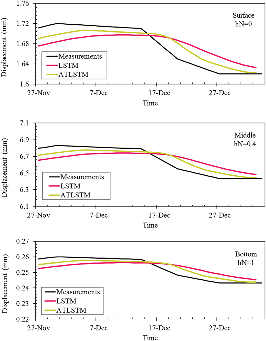
Figure 18: Comparative analysis of prediction results for LSTM and ATLSTM models

Fig. 19 depicts the attention scores as a contour map for ES1’s test data. The lookback window indicates which past data points within the set window size were predominantly focused during learning. A lookback window of 0 corresponds to data from the previous day, with increasing numbers indicating progressively older data. Fig. 19a shows the scenario when the window size is set to 5. In this case, data from three days prior appears to have the most influence, with attention scores relatively high between two to four days prior, and significantly lower weights assigned to data from one day prior or beyond five days. Fig. 19b presents a window size set to 10, where the focus is on data from four days prior, with lower attention scores assigned to the most recent day and data after seven days. These findings confirm that ATLSTM optimizes performance by enabling the model to select and process the most relevant information from the input sequence while discarding non-essential data, thereby focusing on key details. This approach significantly enhances the model’s effectiveness.

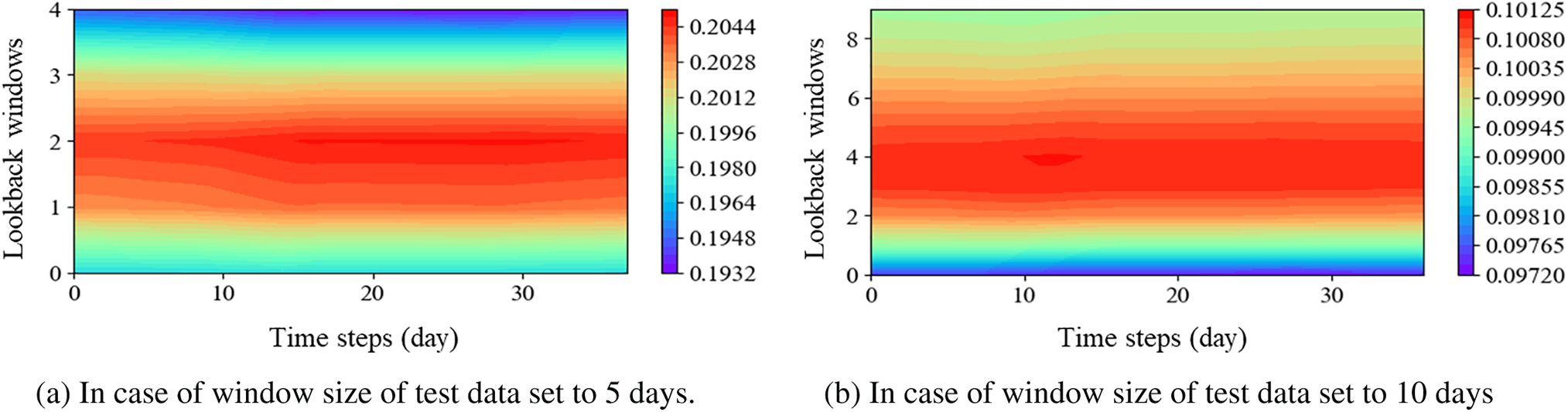
Figure 19: Attention score visualization for ATLSTM in test data of excavation site #1 (ES1)

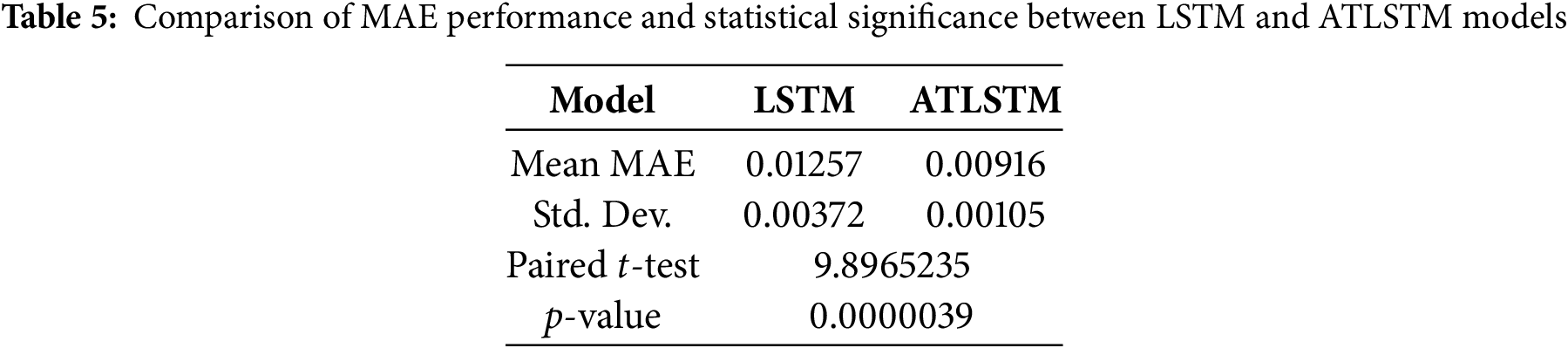
To verify whether the observed performance improvement of ATLSTM over LSTM is statistically significant and not due to random variance, a paired t-test was conducted using the MAE values collected from ten repeated experiments under the same conditions. Table 5 summarizes the mean and standard deviation of the MAE for both models. The LSTM model achieved an average MAE of 0.01257 with a standard deviation of 0.00372, while the ATLSTM model demonstrated a lower average MAE of 0.00916 with a smaller deviation of 0.00105. The paired t-test yielded a t-statistic of 9.897 and a p-value of 0.0000039, which is well below the significance level of 0.05. This result confirms that the performance gain of ATLSTM over the baseline LSTM model is statistically significant. Therefore, it can be concluded that the attention mechanism incorporated in ATLSTM plays a crucial role in improving prediction accuracy by enabling the model to focus on more informative time steps in the input sequence. These findings provide strong evidence that the enhanced performance of ATLSTM is not a result of random variation but a reliable improvement attributed to the attention structure. This justifies the use of ATLSTM for more accurate and stable predictions in time-series deformation monitoring of earth-retaining walls.

4.5 Generalization Performance Comparison between LSTM and ATLSTM

In this study, we tested the performance of LSTM and Attention-Enhanced LSTM (ATLSTM) models trained on time series data from excavation site ES1 when applied to new sites, ES2 and ES3, to evaluate if they maintained consistent performance. Fig. 20 illustrates the results of applying the LSTM and ATLSTM, trained on ES1’s data, to the complete datasets of new sites ES2 and ES3, with performance indicators detailed in Table 6. In all instances, ATLSTM exhibited superior performance. Notably, at ES2, where the most significant displacement occurred at hN = 0.4, the MAPE for LSTM was 21.2106% compared to 5.9002% for ATLSTM, highlighting a significant improvement. Similarly, at ES3, the MAPE was 5.0654% for LSTM and 1.3489% for ATLSTM, confirming ATLSTM’s enhanced performance at consistent depth. While the time series data pattern at ES3 generally increased and then plateaued, mirroring that of ES1, ES2 displayed a pattern of consistent increase with greater volatility. Both models showed high performance when applied to ES3. A notable observation was that both models exhibited some initial error due to the characteristic of LSTM models learning from sequence data patterns, which typically show lower performance initially due to insufficient data but improve over time. Implementing the attention mechanism can be particularly effective in these scenarios.

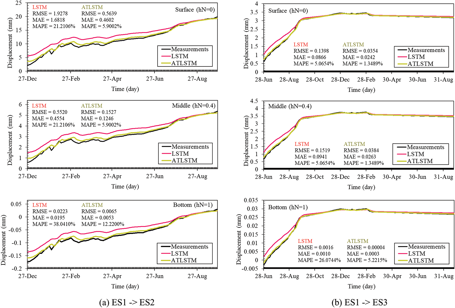
Figure 20: Comparative analysis of prediction results for LSTM and ATLSTM models

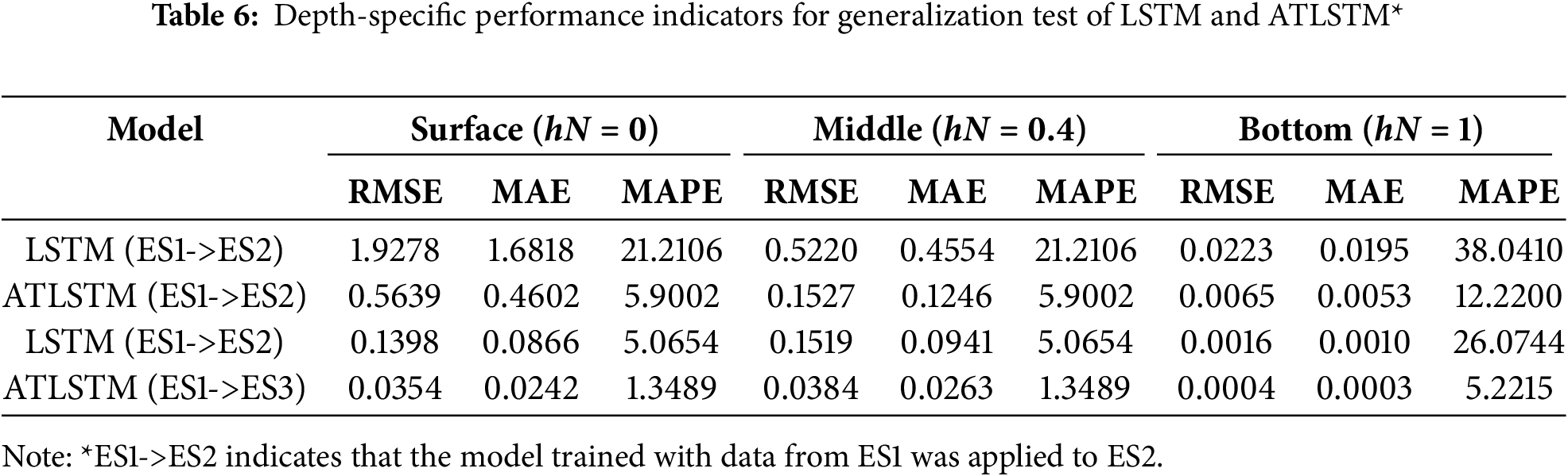
Fig. 21 displays the attention scores when ATLSTM was applied to the test datasets of ES2 and ES3. The lookback window size (W) was set to 10. For ES2, initially focusing on data from three days prior, adjustments to the attention scores were made as data volatility increased over time, as shown in Fig. 21a. In the case of ES3, where the data pattern increased gradually without significant volatility, initial focus was on data from five days prior, shifting to a concentration on data from ten days prior as slight decreases occurred in later data, as illustrated in Fig. 21b. This adaptive focus on relevant historical data by ATLSTM underscores its capability to dynamically adjust to changing data patterns and enhance predictive accuracy.

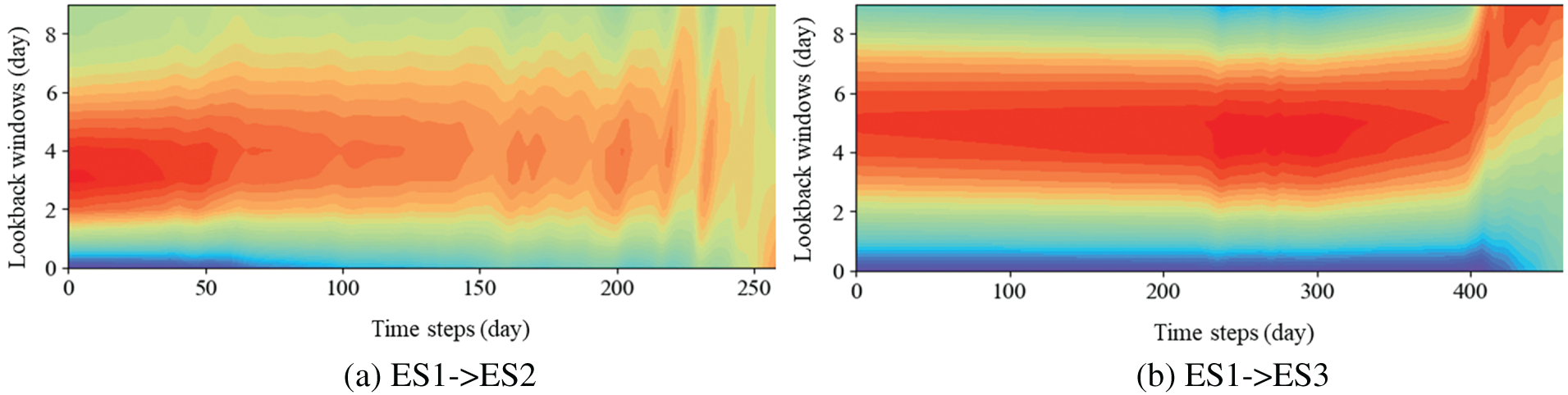
Figure 21: Attention score visualization for ATLSTM in test data of excavation site #2, 3 (ES2, 3)

4.6 Prediction Results for ERWs Deformation Profiles

In this research, the effects of using ARIMA, LSTM, and ATLSTM models to predict overall deformation in ERWS were explored. Fig. 22 synthesizes the predictions made from depth-specific sensor data to illustrate the deformation profiles of earth-retaining walls. For each site’s test data, data at four specific times (A, B, C, D) were extracted to assess the models over time. For ES1, where a substantial amount of training data was available, all three models performed well; however, ARIMA showed effectiveness in short-term predictions, with errors increasing over time. In contrast, LSTM and ATLSTM managed to predict with high accuracy and stability throughout the period. For ES2, characterized by strong non-stationarity where past trends do not repeat, ARIMA exhibited significant prediction errors. LSTM showed initially low accuracy, which improved over time, while ATLSTM consistently maintained high performance both short and long term. Notably, the deformation profile of ES2 did not conform to the typical lateral displacement curves commonly expected in geotechnical engineering. This irregularity is likely due to field-induced uncertainties such as inclinometer casing twist, improper installation, or delayed bracing, which can introduce noise into the measured data. Despite this irregular and noisy nature of the time-series data, the proposed models—especially ATLSTM—demonstrated robust predictive capability, effectively capturing complex deformation trends that deviate from conventional expectations. The outcomes for ES3 also reflected the distinct characteristics of each model. ARIMA displayed errors, particularly in parts of the time series with high volatility (points B and C), whereas LSTM and ATLSTM showed consistently strong performance. In sections A, B, and C of ES3, which displayed gradual increases similar to past patterns, ARIMA’s errors were not substantial.

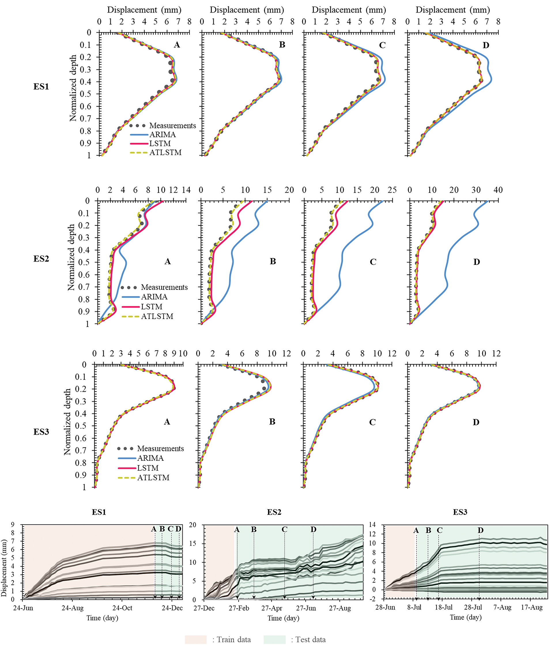
Figure 22: Prediction results for earth retaining wall deformation using ARIMA, LSTM, ATLSTM models

Inclinometer measurements for ERW displacement are predominantly non-stationary, indicating that recent data most accurately explains current conditions, with correlations decreasing as one goes further back in time. Under such circumstances, ARIMA, which assumes linearity, tends to lose predictive accuracy. While transformations such as differencing can be applied to overcome this limitation, ensuring long-term accuracy requires continual adjustments and updates to the model’s parameters. On the other hand, LSTM handles the complexity and non-stationarity of sequence data effectively, especially showing high performance in long-term predictions. Integrating the attention mechanism into LSTM allows for differential importance to be assigned to data points, focusing on more crucial information, thereby enhancing both short and long-term predictive performance. This adaptive weighting proves extremely beneficial at points in the time series where data patterns undergo significant changes.

5  Limitation and Future Works

This study proposed a deformation prediction model for earth-retaining walls (ERWs) using only the time series data from inclinometers installed during construction. By focusing exclusively on sensor-derived temporal data, the model minimized uncertainties stemming from a wide range of input variables, which are commonly required in traditional numerical or data-driven approaches. As such, the proposed method demonstrated practical feasibility for monitoring wall deformation in real-time construction settings, offering a lightweight and deployable alternative to complex input-dependent models. However, several limitations remain. First, the exclusion of ground investigation data (e.g., shear strength, unit weight, groundwater level) and structural parameters makes the model less suitable for use in the design stage, where detailed geotechnical assessments and safety factor evaluations are required. While this simplification is advantageous for field applicability, it limits the interpretability and diagnostic utility of the model, especially when attempting to identify the underlying causes of unusual wall movements. Second, although the model achieved promising accuracy across three monitored sites, its generalization capability to unseen excavation sites remains a challenge. The current model is trained on a limited dataset representing a narrow range of geotechnical and construction conditions. For broader applicability, future work must incorporate a wider variety of excavation cases, including those involving different ground types, support systems, and construction methods. Notably, in Fig. 22, the deformation pattern of Site ES2 deviated from the typical lateral displacement shape expected in geotechnical behavior. This atypical time series is suspected to contain field-induced noise, possibly due to casing twist, inclinometer misalignment, or delays in support installation. Despite these irregularities, the proposed ATLSTM model maintained relatively stable performance, suggesting its robustness against measurement noise. This is likely attributable to the attention mechanism’s inherent capability to focus on informative time steps while down-weighting irrelevant or noisy segments. However, this hypothesis was inferred based on prediction accuracy and qualitative evaluation. A more rigorous assessment of the model’s robustness under varying noise levels will be explored in future research. Additionally, the current model has not been trained on datasets representing failure scenarios. While typical excavation sites are managed to prevent instability, wall collapse or failure cases may exhibit fundamentally different time series behavior. As such, future work should explore the inclusion of anomalous or failure-condition data to enhance the model’s capacity for early warning or risk detection. Finally, the model’s applicability under seismic loading conditions has not been addressed in this study. Given the increasing importance of seismic resilience in geotechnical design, incorporating earthquake-related parameters and evaluating model performance under seismic excitation remains a significant direction for future research. In summary, while the proposed approach contributes to simplifying and improving real-time monitoring of ERW deformation using inclinometer time series, further research is needed to improve generalization, interpretability, and robustness, particularly under extreme or atypical conditions.

6  Conclusion

In this study, we utilized inclinometer measurement data from excavation sites to construct and compare two prediction models: ARIMA and LSTM. The aim was to assess the stability of ERWs and predict future displacements through time series analysis, examining the differences between traditional statistical-based approaches and deep learning methods and aiming to enhance their accuracy. The main conclusions drawn from the study are as follows:

(1)   Across various tests, the LSTM consistently outperformed the ARIMA, especially in long-term predictions. This indicates that LSTM is capable of effectively modeling the nonlinear patterns and long-term dependencies inherent in time series data.

(2)   An analysis of the impact of sequence length on the performance of both models showed that as sequence length increased, the LSTM demonstrated more pronounced improvements in prediction performance. In contrast, the ARIMA showed limited enhancement in long-term prediction capabilities with longer sequence lengths. Therefore, for long-term predictions of subsurface displacement changes, the LSTM appears more suitable.

(3)   Although the LSTM exhibited some shortcomings in short-term predictions, these were mitigated through data augmentation techniques such as up-sampling. This allowed the LSTM to demonstrate high flexibility and adaptability in both short and long-term predictions, making it a robust predictive tool capable of accommodating various changes at the excavation sites.

(4)   While the ARIMA shows strengths in short-term predictions, it has limitations in handling non-stationary data and requires continual model updates. On the other hand, the LSTM effectively processes non-stationary data and can enhance both its short- and long-term predictive performance as well as its generalization capabilities through data augmentation and the application of attention mechanisms. Particularly for time series data with high volatility and changing patterns, using ATLSTM can prioritize crucial data points, significantly improving prediction accuracy.

Therefore, in practical settings like excavation site monitoring, utilizing LSTM could be more effective. Real-time monitoring and prediction using LSTM can enhance the efficiency of excavation operations and enable swift decision-making based on predictive insights, potentially minimizing property damage and reducing the risk of casualties.

Acknowledgement: None.

Funding Statement: Research for this paper was carried out under the KICT Research Program (Project No. 20250285-001, Development of Infrastructure Disaster Prevention Technology Based on Satellites SAR) funded by the Ministry of Science and ICT.

Author Contributions: Seunghwan Seo: Conceptualization, Methodology, Validation, Formal analysis, Investigation, Writing—original draft, Software, Visualization. Moonkyung Chung: Resources, Writing—review & editing, Supervision. All authors reviewed the results and approved the final version of the manuscript.

Availability of Data and Materials: The datasets generated during the current study are available from the corresponding author on reasonable request.

Ethics Approval: Not applicable.

Conflicts of Interest: The authors declare no conflicts of interest to report regarding the present study.

References

1. Peck RB. Deep excavations and tunneling in soft ground. In: Proceedings of the 7th International Conference on Soil Mechanics and Foundation Engineering; 1969 Aug 25–29; Mexico City, Mexico. p. 225–90. [Google Scholar]

2. Hsiung BB. Observations of the ground and structural behaviours induced by a deep excavation in loose sands. Acta Geotech. 2020;15(6):1577–93. doi:10.1007/s11440-019-00864-0. [Google Scholar] [CrossRef]

3. Lim A, Ou CY, Hsieh PG. Investigation of the integrated retaining system to limit deformations induced by deep excavation. Acta Geotech. 2018;13(4):973–95. doi:10.1007/s11440-017-0613-6. [Google Scholar] [CrossRef]

4. Long M. Database for retaining wall and ground movements due to deep excavations. J Geotech Geoenviron Eng. 2001;127(3):203–24. doi:10.1061/(asce)1090-0241(2001)127:3(203). [Google Scholar] [CrossRef]

5. Meng FY, Chen RP, Wu HN, Xie SW, Liu Y. Observed behaviors of a long and deep excavation and collinear underlying tunnels in Shenzhen granite residual soil. Tunn Undergr Space Technol. 2020;103(6):103504. doi:10.1016/j.tust.2020.103504. [Google Scholar] [CrossRef]

6. Moormann C. Analysis of wall and ground movements due to deep excavations in soft soil based on a new worldwide database. Soils Found. 2004;44(1):87–98. doi:10.3208/sandf.44.87. [Google Scholar] [CrossRef]

7. Clough GW, O’Rourke TD. Construction induced movements of in situ walls. In: proceedings of the Specialty Conference on Design and Performance of Earth Retaining Structures; 1990 Jun 18–21; Ithaca, NY, USA. p. 439–70. [Google Scholar]

8. Lee SJ, Song TW, Lee YS, Song YH, Kim HK. A case study of building damage risk assessment due to the multi-propped deep excavation in deep soft soil. In: Soft Soil Engineering: Proceedings of the Fourth International Conference on Soft Soil Engineering. Abingdon, UK: Talylor Francis Group; 2007. [Google Scholar]

9. Son M, Cording EJ. Estimation of building damage due to excavation-induced ground movements. J Geotech Geoenviron Eng. 2005;131(2):162–77. doi:10.1061/(asce)1090-0241(2005)131:2(162). [Google Scholar] [CrossRef]

10. Son M, Cording EJ. Evaluation of building stiffness for building response analysis to excavation-induced ground movements. J Geotech Geoenviron Eng. 2007;133(8):995–1002. doi:10.1061/(asce)1090-0241(2007)133:8(995). [Google Scholar] [CrossRef]

11. Lam SY, Haigh SK, Bolton MD. Understanding ground deformation mechanisms for multi-propped excavation in soft clay. Soils Found. 2014;54(3):296–312. doi:10.1016/j.sandf.2014.04.005. [Google Scholar] [CrossRef]

12. Finno RJ, Arboleda-Monsalve LG, Sarabia F. Observed performance of the one museum park west excavation. J Geotech Geoenviron Eng. 2015;141(1):04014078. doi:10.1061/(asce)gt.1943-5606.0001187. [Google Scholar] [CrossRef]

13. Cui J, Yang Z, Azzam R. Field measurement and numerical study on the effects of under-excavation and over-excavation on ultra-deep foundation pit in coastal area. J Mar Sci Eng. 2023;11(1):219. doi:10.3390/jmse11010219. [Google Scholar] [CrossRef]

14. Zheng G, Guo Z, Zhou H, Tan Y, Wang Z, Li S. Multibench-retained excavations with inclined-vertical framed retaining walls in soft soils: observations and numerical investigation. J Geotech Geoenviron Eng. 2024;150(5):05024003. doi:10.1061/jggefk.gteng-11943. [Google Scholar] [CrossRef]

15. Li MG, Xiao X, Wang JH, Chen JJ. Numerical study on responses of an existing metro line to staged deep excavations. Tunn Undergr Space Technol. 2019;85(6):268–81. doi:10.1016/j.tust.2018.12.005. [Google Scholar] [CrossRef]

16. Hou YM, Wang JH, Zhang LL. Finite-element modeling of a complex deep excavation in Shanghai. Acta Geotech. 2009;4(1):7–16. doi:10.1007/s11440-008-0062-3. [Google Scholar] [CrossRef]

17. Hsieh PG, Ou CY. Shape of ground surface settlement profiles caused by excavation. Can Geotech J. 1998;35(6):1004–17. doi:10.1139/t98-056. [Google Scholar] [CrossRef]

18. Li MG, Xiao QZ, Liu NW, Chen JJ. Predicting wall deflections for deep excavations with servo struts in soft clay. J Geotech Geoenviron Eng. 2024;150(1):04023124. doi:10.1061/jggefk.gteng-11347. [Google Scholar] [CrossRef]

19. Wong IH, Poh TY. Effects of jet grouting on adjacent ground and structures. J Geotech Geoenviron Eng. 2000;126(3):247–56. doi:10.1061/(asce)1090-0241(2000)126:3(247). [Google Scholar] [CrossRef]

20. Zhang W, Goh ATC, Xuan F. A simple prediction model for wall deflection caused by braced excavation in clays. Comput Geotech. 2015;63(4):67–72. doi:10.1016/j.compgeo.2014.09.001. [Google Scholar] [CrossRef]

21. Goh ATC, Zhang RH, Wang W, Wang L, Liu HL, Zhang WG. Numerical study of the effects of groundwater drawdown on ground settlement for excavation in residual soils. Acta Geotech. 2020;15(5):1259–72. doi:10.1007/s11440-019-00843-5. [Google Scholar] [CrossRef]

22. Seo S, Park J, Ko Y, Kim G, Chung M. Geotechnical factors influencing earth retaining wall deformation during excavations. Front Earth Sci. 2023;11:1263997. doi:10.3389/feart.2023.1263997. [Google Scholar] [CrossRef]

23. Goh ATC, Zhang F, Zhang W, Zhang Y, Liu H. A simple estimation model for 3D braced excavation wall deflection. Comput Geotech. 2017;83:106–13. doi:10.1016/j.compgeo.2016.10.022. [Google Scholar] [CrossRef]

24. Kung GTC, Hsiao ECL, Schuster M, Juang CH. A neural network approach to estimating deflection of diaphragm walls caused by excavation in clays. Comput Geotech. 2007;34(5):385–96. doi:10.1016/j.compgeo.2007.05.007. [Google Scholar] [CrossRef]

25. Goh ATC, Wong KS, Broms BB. Estimation of lateral wall movements in braced excavations using neural networks. Can Geotech J. 1995;32(6):1059–64. doi:10.1139/t95-103. [Google Scholar] [CrossRef]

26. Zhang W, Zhang R, Wu C, Goh ATC, Lacasse S, Liu Z, et al. State-of-the-art review of soft computing applications in underground excavations. Geosci Front. 2020;11(4):1095–106. doi:10.1016/j.gsf.2019.12.003. [Google Scholar] [CrossRef]

27. Zhang R, Wu C, Goh ATC, Böhlke T, Zhang W. Estimation of diaphragm wall deflections for deep braced excavation in anisotropic clays using ensemble learning. Geosci Front. 2021;12(1):365–73. doi:10.1016/j.gsf.2020.03.003. [Google Scholar] [CrossRef]

28. Seo S, Chung M. Development of an ensemble prediction model for lateral deformation of retaining wall under construction. J Korean Geotechnical Society. 2023;39(4):5–17. doi:10.7843/kgs.2023.39.4.5. [Google Scholar] [CrossRef]

29. Sheini Dashtgoli D, Dehnad MH, Ahmad Mobinipour S, Giustiniani M. Performance comparison of machine learning algorithms for maximum displacement prediction in soldier pile wall excavation. Undergr Space. 2024;16(8):301–13. doi:10.1016/j.undsp.2023.09.013. [Google Scholar] [CrossRef]

30. Johari A, Javadi AA, Najafi H. A genetic-based model to predict maximum lateral displacement of retaining wall in granular soil. Sci Iran. 2016;23(1):54–65. doi:10.24200/sci.2016.2097. [Google Scholar] [CrossRef]

31. Yang B, Yin K, Lacasse S, Liu Z. Time series analysis and long short-term memory neural network to predict landslide displacement. Landslides. 2019;16(4):677–94. doi:10.1007/s10346-018-01127-x. [Google Scholar] [CrossRef]

32. Mahmoodzadeh A, Mohammadi M, Daraei A, Farid Hama Ali H, Kameran Al-Salihi N, Mohammed Dler Omer R. Forecasting maximum surface settlement caused by urban tunneling. Autom Constr. 2020;120:103375. doi:10.1016/j.autcon.2020.103375. [Google Scholar] [CrossRef]

33. Yang M, Song M, Guo Y, Lyv Z, Chen W, Yao G. Prediction of shield tunneling-induced ground settlement using LSTM architecture enhanced by multi-head self-attention mechanism. Tunn Undergr Space Technol. 2025;161(9):106536. doi:10.1016/j.tust.2025.106536. [Google Scholar] [CrossRef]

34. Zhao HJ, Liu W, Shi PX, Du JT, Chen XM. Spatiotemporal deep learning approach on estimation of diaphragm wall deformation induced by excavation. Acta Geotech. 2021;16(11):3631–45. doi:10.1007/s11440-021-01264-z. [Google Scholar] [CrossRef]

35. Seo S, Chung M. Evaluation of applicability of 1D-CNN and LSTM to predict horizontal displacement of retaining wall according to excavation work. Int J Adv Comput Sci Appl. 2022;13(2):86–91. doi:10.14569/ijacsa.2022.0130210. [Google Scholar] [CrossRef]

36. Wu C, Hong L, Wang L, Zhang R, Pijush S, Zhang W. Prediction of wall deflection induced by braced excavation in spatially variable soils via convolutional neural network. Gondwana Res. 2023;123(6):184–97. doi:10.1016/j.gr.2022.06.011. [Google Scholar] [CrossRef]

37. Kalantari AR, Johari A. System reliability analysis for seismic stability of the soldier pile wall using the conditional random finite-element method. Int J Geomech. 2022;22(10):04022159. doi:10.1061/(asce)gm.1943-5622.0002534. [Google Scholar] [CrossRef]

38. Shan J, Zhang X, Liu Y, Zhang C, Zhou J. Deformation prediction of large-scale civil structures using spatiotemporal clustering and empirical mode decomposition-based long short-term memory network. Autom Constr. 2024;158(4):105222. doi:10.1016/j.autcon.2023.105222. [Google Scholar] [CrossRef]

39. Yang C, Wang C, Zhao F, Wu B, Fan JS, Zhang Y. Smart virtual sensing for deep excavations using real-time ensemble graph neural networks. Autom Constr. 2025;172:106040. doi:10.1016/j.autcon.2025.106040. [Google Scholar] [CrossRef]

40. Liu W, Tong L, Li H, Wang Z, Sun Y, Gu W. Multi-parameter intelligent inverse analysis of a deep excavation considering path-dependent behavior of soils. Comput Geotech. 2024;174(S2):106597. doi:10.1016/j.compgeo.2024.106597. [Google Scholar] [CrossRef]

41. Box GEP, Jenkins GM, Reinsel GC, Ljung GM. Time series analysis: forecasting and control. 5th ed. Hoboken, NJ, USA: John Wiley & Sons; 2015. [Google Scholar]

42. Suhermi N, Suhartono, Permata RP, Rahayu SP. Forecasting the search trend of muslim clothing in Indonesia on google trends data using ARIMAX and neural network. In: Soft computing in data science. Singapore: Springer; 2019. p. 272–86. doi:10.1007/978-981-15-0399-3_22. [Google Scholar] [CrossRef]

43. Hochreiter S, Schmidhuber J. Long short-term memory. Neural Comput. 1997;9(8):1735–80. doi:10.1162/neco.1997.9.8.1735. [Google Scholar] [PubMed] [CrossRef]

44. Bahdanau D, Chorowski J, Serdyuk D, Brakel P, Bengio Y. End-to-end attention-based large vocabulary speech recognition. In: 2016 IEEE International Conference on Acoustics, Speech and Signal Processing (ICASSP); 2016 Mar 20–25; Shanghai, China. p. 4945–9. doi:10.1109/ICASSP.2016.7472618. [Google Scholar] [CrossRef]

45. Pascanu R, Mikolov T, Bengio Y. On the difficulty of training recurrent neural networks. In: 30th International Conference on Machine Learning; 2013 Jun 16–21; Atlanta, GA, USA. p. 1310–8. doi:10.5555/3042817.3043083. [Google Scholar] [CrossRef]

46. Dunnicliff J. Geotechnical instrumentation for monitoring field performance. Hoboken, NJ, USA: John Wiley & Sons, Inc.; 1988. [Google Scholar]

47. Li S, Li Q, Cook C, Zhu C, Gao Y. Independently recurrent neural network (IndRNNbuilding a longer and deeper RNN. In: Proceedings of the 2018 IEEE Conference on Computer Vision and Pattern Recognition; 2018 Jun 18–23; Salt Lake City, UT, USA. p. 5457–66. doi:10.48550/arXiv.1803.04831. [Google Scholar] [CrossRef]

48. Semenoglou AA, Spiliotis E, Assimakopoulos V. Data augmentation for univariate time series forecasting with neural networks. Pattern Recognit. 2023;134(3):109132. doi:10.1016/j.patcog.2022.109132. [Google Scholar] [CrossRef]