
 Submit a Paper
 Propose a Special lssue
 Open Access
ARTICLE

Numerical Study on the Icing Characteristics of Flat Plates and Its Influencing Factors
1 Department of Bridge Engineering, Southwest Jiaotong University, Chengdu, 610031, China
2 State Key Laboratory of Bridge Intelligent and Green Construction, Southwest Jiaotong University, Chengdu, 611756, China
* Corresponding Author: Jin Zhu. Email:
Computer Modeling in Engineering & Sciences 2025, 144(3), 2849-2872. https://doi.org/10.32604/cmes.2025.070287
Received 12 July 2025; Accepted 29 August 2025; Issue published 30 September 2025
 View Full Text
 Download PDF
Abstract
Ice accretion on structures such as aircraft wings and wind turbine blades poses serious risks to aerodynamic performance and operational safety, particularly in cold and humid environments. This study conducts numerical simulations of ice formation on thin flat plates using CFD and FENSAP-ICE, exploring how air temperature, wind velocity, and angle of attack (AOA) affect icing behavior and aerodynamic characteristics. Results indicate that ice thickness increases linearly over time. Rime ice forms at low temperatures due to immediate droplet freezing, whereas glaze ice develops at higher temperatures when a water film forms and subsequently refreezes into protruding ice horns; under identical conditions, rime ice consistently produces thicker ice layers than glaze ice. Increasing wind speed substantially enhances ice growth and coverage, while speeds as low as 1 m/s result in minimal accretion. Changes in AOA shift the icing region toward the pressure side, and AOAs of equal magnitude but opposite sign yield symmetrical ice accretion patterns and identical maximum thickness values. After icing, the plate’s leading edge becomes smoother, slightly reducing drag while increasing lift and moment coefficients. These findings highlight the dominant roles of temperature, wind speed, and AOA in determining ice morphology, extent, and aerodynamic impact, providing valuable insights for predicting icing effects and developing mitigation strategies for structures operating in icing-prone regions.Keywords
Owing to its vast geographic extent, China spans regions with highly diverse and contrasting climatic conditions. In the far north, winter temperatures in Heilongjiang Province frequently fall below −15°C, whereas the Qinghai-Tibet Plateau in the west is distinguished by pronounced diurnal temperature variations and the influence of complex topography. These conditions lead to road icing, a major traffic safety hazard, which has been prioritized by the China Meteorological Administration for early warning systems [1]. Road icing significantly reduces tire friction, impairing vehicle handling and braking, and increasing the risk of accidents [2]. A notable example is the 28 December 2009, incident on the Poyang Lake Bridge on the Hangrui Expressway, where low temperatures and dense fog caused multiple collisions, endangering lives and property. Beyond road infrastructure, the issue of icing extends to other critical engineering applications, such as aviation. With the rapid development of China’s aerospace industry, ice accumulation on aircraft during flight has raised serious safety concerns. Icing disrupts smooth airflow, increases drag, raises the critical stall speed, and reduces control efficiency, ultimately threatening flight safety [3]. Similarly, in the wind power sector, extreme weather conditions, particularly in inland areas like Chongqing, Yunnan, and Hunan, have led to severe ice buildup on wind turbine blades. This not only reduces power output and annual energy production (AEP) by up to 17% but also degrades aerodynamic performance by 20% to 50%, and in some cases, even results in turbine shutdowns [4,5]. Data from a Finnish wind farm revealed that icing accounted for 70% of downtime during 1996–2002 [6–8]. The issue of icing is therefore of paramount importance across a wide range of engineering disciplines. As a fundamental aerodynamic shape used in various structures, flat plates commonly appear in applications such as ships, large wind turbine blades, and bridge designs, posing unique challenges in icing behavior. Investigating these challenges is crucial for improving safety, optimizing energy efficiency, and advancing engineering applications.
1.2.1 Aviation and Wind Turbine Fields (Dominant Fields)
Ice accretion is a complex three-dimensional phenomenon that involves multiphase flow, latent heat transfer, phase changes, as well as the influence of gravitational, viscous, and shear forces. Current research on ice accretion primarily focuses on the icing of aircraft and large wind turbines. In the aviation field, Cao et al. [9,10] developed a numerical simulation method based on Eulerian two-phase flow theory to predict ice accretion on airfoils and wings. They initially studied ice formation on the NACA0012 airfoil and the GLC-305 wing model, and later extended their work by incorporating a Eulerian droplet collision method and a heat transfer model to simulate three-dimensional ice accretion, investigating the impact of meteorological parameters. Feng et al. [11] analyzed the aerodynamic characteristics of airfoils with different ice shapes (none, rime, mixed) using computational fluid dynamics (CFD) simulations, finding that ice shape significantly affects lift and drag coefficients. Lian et al. [12] proposed a modified spongy icing model that incorporates the effect of water droplet retention on the ice accretion process. The model, verified through CFD simulations and experimental data on a NACA0012 airfoil, shows improved accuracy in predicting ice accretion morphology, particularly under conditions where liquid water is present at higher temperatures. Dai et al. [13] developed a phase-field-based ice accretion model to predict ice shape on aircraft surfaces, demonstrating its ability to accurately simulate ice formation under various icing conditions. Zheng et al. [14] investigated the impact of four design parameters on airfoil lift and drag coefficients using a simplified ridge ice model, finding that the height of the upper ice horn had the greatest effect, followed by the angle and location of the upper ice horn. Bhatia and al Wahaibi [15] numerically studied the impact of three ice accretion patterns on airfoil performance, finding that ice accretion can reduce lift by 75.3% and increase drag by 280%, with performance loss depending on ridge height, ice thickness, and extent of accretion. Liu and Hu [16] conducted experimental research on unsteady heat transfer and dynamic ice accretion processes on the NACA 0012 airfoil under different icing conditions. Wu et al. [17] developed a 3D numerical method to study icing characteristics in aeroengine stage 35 compressors, finding that icing significantly impacts compressor performance, with rime ice transitioning to glaze ice and causing flow obstruction, particularly at the leading edge. Nogi and Imamura [18] developed a 2D/3D numerical model using the rigid sphere model (RSM) and CFD to predict rime ice accretion on airfoils, with results validated by NASA wind tunnel experiments. Cao & Xin [19] and Shad and Sherif [20] developed a numerical model for simulating ice accretion on two-dimensional airfoil surface under supercooled large droplet (SLD) conditions. In summary, significant progress has been made in the study of aircraft icing, covering various aspects such as icing mechanisms, numerical simulation techniques, and de-icing technologies. These studies have provided essential theoretical foundations and technical support for ensuring flight safety. In terms of anti-icing system design, recent work has examined the influence of key geometric parameters, such as jet arrangement, impingement angle, and piccolo-tube positioning, on the thermal efficiency of hot-air systems for partial-span wings [21]. In parallel, intelligent prediction methods integrating artificial neural networks with IoT (Internet of Things) platforms have been proposed to enable real-time thermal performance forecasting and control for wing anti-icing systems [22]. In addition, Song et al. [23,24] applied peridynamics to simulate thermo-mechanical ice removal, capturing fracture and detachment processes beyond the capability of conventional finite element methods. They further introduced a modified ice failure criterion to improve prediction accuracy under combined thermal and mechanical loads, offering new insights for efficient de-icing strategies.
In the field of wind energy, several studies have investigated the impact of icing on wind turbine blades. Li et al. [25] developed a quasi-3D computational method to analyze the effects of temperature on ice accretion near the blade tips of large-scale horizontal-axis wind turbines. Their numerical simulations revealed that temperature variations significantly influence the distribution and characteristics of ice accretion, which can adversely affect turbine performance. Zhang et al. [26] conducted a numerical simulation of rime ice accretion on a 3D wind turbine blade using the Lagrangian approach, revealing that the ice accretion severity increases near the blade tip and varies radially. Guan et al. [27] investigated the effect of ice roughness on the performance of wind turbine blades, finding that hard rime ice has a more significant aerodynamic impact than soft rime ice, and that surface roughness plays a crucial role in the formation of soft rime ice and its subsequent aerodynamic performance. Dai et al. [28] investigated the effect of ice accretion at blade tips on the vibration performance of wind turbines. Their research emphasized the need to consider icing effects in the dynamic analysis of turbine blades to prevent potential structural issues. Wang and Zhu [29] investigated the ice accretion on 3D wind turbine blades and found that in-cloud icing primarily occurs near the leading edge, with icing thickness and extent increasing along the spanwise length. Manatbayev et al. [30] proposed a numerical method to predict ice accretion shapes on vertical axis wind turbine (VAWT) blades under varying angles of attack, finding that rime ice causes minimal aerodynamic impact, while glaze ice leads to significant flow separation and a 60% reduction in power performance. Collectively, these studies underscore the critical need for accurate icing simulations to assess and mitigate the adverse effects of ice accretion on wind turbine performance.
In the field of bridge engineering, Chen et al. [31] developed a finite element model to predict ice accretion on bridge deck pavements, incorporating meteorological, structural, and traffic factors. They found that air temperature and water accumulation significantly affect freezing. Yang et al. [32] developed a model to predict the icing time and thickness on bridge pavements under low solar radiation (rainy conditions) and analyze the effects of external factors including ambient temperature, wind speed, and water depth on icing. Li et al. [33] investigated ice accumulation on stay cables, finding that lower temperatures promote icicle growth, while larger diameter and steeper inclination angles inhibit it. Xu and Yu et al. [34–36] conducted comprehensive studies on pipeline suspension bridges using icing and wind tunnel experiments. They investigated the effects of ice accretion on aerodynamic and structural performance, providing crucial data for the wind-resistant design of similar bridges in cold regions. Górski et al. [37] conducted wind tunnel tests on an iced cable model for cable-stayed bridges, and found that the ice accretion on the cable model has a significant influence on the aerodynamic forces acting on the model. Additionally, Tang et al. [38] developed a numerical simulation method for ice accretion on helicopter rotor blades. Fu et al. [39] used 3D simulations to study the effects of rotational speed on droplet impingement and ice accretion on rotating engine components under supercooled large droplet conditions. Zhou and Yin [40] presented a numerical study on glaze ice accretion on cables considering the effects of in-plane motions of cable on the glaze icing process. To tackle with the icing on transmission lines, Liu et al. [41] developed a “point-line-face-solid” ice shape reconstruction algorithm to realize three-dimensional numerical simulation of rime ice accretion on the insulator.
While significant research has focused on ice accretion in aviation and wind turbines, studies specifically targeting ice formation on flat plates are relatively limited. Flat plates are commonly found in various engineering applications, such as aircraft wings, wind turbine blades, turbine blades, reactor fuel plates, bridge wind-resistant designs, and large fan blades, which typically feature flat or quasi-flat cross-sections [42]. Despite their widespread use, the fundamental mechanisms, quantitative characteristics, and aerodynamic consequences of ice accretion on flat plates remain insufficiently documented in the literature. Most existing icing research has concentrated on complex geometries or curved surfaces, where the dynamics of ice formation are more intricate. In contrast, flat plates, though simpler in geometry, present distinct aerodynamic and thermodynamic challenges for accurately predicting ice growth and its influence on performance. Key parameters, including the effects of wind speed, angle of attack, and temperature on ice accretion, remain relatively underexplored for flat plates. Addressing these gaps is essential for developing predictive icing models applicable to a broad range of engineering systems. Therefore, in-depth research on the icing characteristics of flat plates and their impact on aerodynamic performance is crucial for improving the safety and reliability of structures operating in cold and humid environments.
1.4 Aim and Structure of the Work
This study aims to address the identified gap by establishing a validated numerical framework to investigate the coupled influence of key environmental parameters on flat plate icing behavior and its aerodynamic implications. The work provides deeper insights into the mechanisms governing ice formation and growth under controlled variations in temperature, wind speed, and AOA, thereby contributing to the development of more accurate and physically informed ice accretion models for practical engineering applications. The methodology integrates computational fluid dynamics (CFD) simulations with the FENSAP-ICE icing module, enabling detailed resolution of the flow field, droplet impingement characteristics, and subsequent ice accretion morphology. Section 2 introduces the physical mechanisms of icing and outlines the proposed four-step numerical framework: grid generation, flow field calculation, droplet impingement analysis, and ice accretion simulation using a “quasi-steady” approach. Section 3 validates the numerical framework against experimental data, establishing confidence in its predictive capability. Section 4 presents the simulation results regarding the icing characteristics of flat plates, focusing on the effects of air temperature, wind velocity, and angle of attack on ice accretion. In addition, the section quantifies the impact of different ice accretion scenarios on static aerodynamic coefficients, providing a direct link between environmental conditions and aerodynamic performance. Finally, Section 5 summarizes the key conclusions and highlights the broader engineering implications of the findings.
2 Icing Mechanism and Numerical Methods
Icing is a common physical phenomenon in nature. Water droplets in the air freeze spontaneously into ice only at temperatures of −40°C under undisturbed conditions. When temperatures range from −40°C to 0°C, the droplets enter a metastable state, known as supercooled droplets. In this state, droplets can remain unfrozen for an extended period without external disturbance. However, when disturbances such as contact with cold surfaces, mechanical impacts, or vibrations occur, the droplets freeze, leading to ice formation [43]. In natural environments with lower temperatures and higher humidity, supercooled water droplets inevitably collide with and adhere to the surfaces of structures, causing varying degrees of ice accretion. This process is complex and dependent on environmental factors. The overall icing process is schematically shown in Fig. 1, which provides a visual representation of how ice forms under specific conditions. For the purposes of this study, the focus is on thin flat plates, a common engineering structure in applications such as aircraft wings, turbine blades, and bridges. These plates serve as a representative model for the types of structures subjected to icing in cold and humid environments. The icing phenomena under investigation here are categorized as atmospheric icing, which can be classified based on two main formation processes: precipitation icing and in-cloud icing. According to the international standard ISO 12494: 2017 [44], precipitation icing can be further divided into glaze (freezing rain or drizzle, where air temperatures are between −10°C and 0°C) and wet snow (with air temperatures between 0°C and 3°C). In contrast, in-cloud icing is primarily influenced by wind speed and temperature and is further categorized into soft rime, hard rime, and glaze ice. These different icing types are illustrated in Fig. 2, which shows how environmental conditions determine the specific icing form. In the present study, the temperature range of interest is below 0°C, with a particular emphasis on in-cloud icing, especially focusing on the formation of soft and hard rime, as well as glaze ice.

Figure 1: Schematic of the icing process

Figure 2: Various ice accretion types under different environmental conditions
A numerical framework is proposed to simulate the formation of glaze and rime ice on flat plates, consisting of four main steps, as shown in Fig. 3. In Step I, structured grids are generated using the pre-processing software ICEM CFD, based on the given geometric structure. These grids serve as the background mesh for the subsequent calculations. Step II involves using the finite element software ANSYS FLUENT 2022 R1 to calculate the flow field around the flat plate, with appropriate boundary conditions and solver settings applied. The flow field in this step is treated as a single-phase flow, due to the extremely low droplet volume fraction (on the order of 10−6), which allows the air and droplet phases to be decoupled [17]. As such, the impact of the droplets on the flow field is negligible. This approach simplifies the process by enabling the air flow to be calculated independently in the flow field module. Step III utilizes the DROP3D module in FENSAP-ICE 2022 R1, where the flow field calculated in Step II is imported to determine the droplet trajectories and the distribution of impacts on the plate surface. In Step IV, the ice accretion process is simulated using a “quasi-steady” approach. This method involves solving the steady-state control equations over small time intervals, where the solution from the previous time step (t) is used as the initial condition for the next time step (t + Δt). This iterative process continues until the full time step is completed, ensuring a more accurate simulation of the ice layer’s growth that closely reflects real-world icing phenomena [20]. Additionally, the ICE3D module in FENSAP-ICE is employed to compute the ice accretion characteristics based on its icing model. As the ice shape develops, its growth is used to update the grid for the subsequent time step, iterating until the complete time step is achieved. In the following three subsections, a more detailed explanation of Steps I–IV will be provided.

Figure 3: Proposed numerical framework to simulate the formation of glaze and rime ice on flat plates
2.2.1 Governing Equations for Air Flow
In atmospheric conditions, supercooled water droplets are influenced by the surrounding airflow as they move and collide with surfaces. Therefore, understanding the airflow distribution around an object is essential before analyzing the droplet impingement characteristics. Due to parallel processing limitations in the FENSAP-ICE flow field module, its computation speed is slower than that of other solvers. Moreover, after ANSYS acquired FENSAP-ICE, the software now provides a comprehensive interface for integrating ANSYS flow field analysis data. As a result, this study employs ANSYS FLUENT 2022 R1, a computational fluid dynamics (CFD) software, to simulate the wind field and generate the necessary flow parameters for subsequent droplet impingement calculations.
In computational fluid dynamics, all simulations are based on the governing equations of fluid mechanics, which include the continuity equation, the momentum equation, and the energy equation. These fundamental equations arise from three key physical principles: the conservation of mass, Newton’s second law, and the conservation of energy. In this study, the airflow is assumed to be low-speed, viscous, and incompressible, behaving as a Newtonian fluid. As such, the energy equation is neglected, and the flow field is governed by the continuity and momentum equations, simplifying the model to the Navier-Stokes (N-S) equations, as presented in [45]:
where i and j denote the two directions of a Cartesian coordinate system; xi and ui denote the coordinates and velocity components along the i-axis; xj and uj denote the coordinates and velocity components along the j-axis; t denotes time; ρa denotes air density; pa denotes air pressure; μa denotes air dynamic viscosity; and fi denotes the body force per unit volume in xi direction.
To simulate the turbulent flow in the CFD model, the SST (Shear-Stress Transport) k-ω turbulence model was adopted for its proven capability in predicting viscous flows. It combines the near-wall accuracy of the k-ω formulation with the free-stream independence of the k-ε model through a blending function that applies the k-ω model close to the wall and transitions to a k-ε like form in the far field [46,47]. This hybrid approach, enhanced by a cross-diffusion term and shear stress transport, offers reliable predictions for flows involving boundary layers, separation, and reattachment, and demonstrates strong performance in complex conditions such as adverse pressure gradients, airfoils, and transonic shock interactions. Its suitability for icing simulations has been confirmed in prior studies. Yassin et al. [48] reported accurate modeling of turbulent flow over iced airfoils, while Bhatia and Al Wahaibi [15] demonstrated its efficiency for quantifying aerodynamic effects of ice accretion using ANSYS Fluent. By leveraging the strengths of both k-ε and k-ω formulations, the SST k-ω model provides a robust and widely validated framework, particularly under low Reynolds number conditions, with governing equations detailed in [49]:
where Pk and Pω denote the production terms; F1 denotes the blending function; and μt denotes the turbulent eddy viscosity. Pk, Pω, F1, and μt are expressed as [47,49]:
where y denotes the distance from the field point to the nearest wall; τij denotes the Reynolds stress tensor; CDkω denotes the cross-diffusion term of equation; Ω denotes the vorticity magnitude; and F2 denotes the blending function. Other specific expressions for the equations are the set of constants corresponding to the Wilcox and SST—inner equations [47,49]. τij, CDkω, Ω, and F2 are expressed as:
2.2.2 Governing Equations for Droplet Impingement
The calculation of droplet impingement characteristics is a crucial prerequisite for the subsequent simulation of icing accretion. Under cold and humid conditions, supercooled liquid droplets carried by moist air are prone to impinge on the structural surfaces. Generally, droplet impingement characteristics refer to the range of droplet impacts, the volume of water impacting the surface, and the distribution of the water quantity at locations such as the leading edges of blades or airfoils [50]. The trajectory of supercooled droplets in the air and their impingement on surfaces is a typical two-phase (gas-liquid) flow problem. Currently, two main methods are used to calculate droplet impingement characteristics, i.e., the Lagrangian method and Eulerian method [51]. The Lagrangian method, which is based on Newton’s second law of motion, tracks the movement of droplets in the air by calculating the forces acting on them and their resulting trajectories, ultimately determining the precise location of their impact on a surface. However, this approach requires tracking the trajectories of numerous droplets, making the process computationally complex and inefficient [52]. In contrast, the Eulerian method, developed from field theory, treats the droplets as a continuous phase [53]. By introducing the droplet volume fraction, it solves the continuity and momentum equations for the droplet phase to obtain the distribution of droplet volume fraction and velocity at various points in the spatial grid, which can then be used to calculate droplet impingement characteristics. Since the Eulerian method focuses on the variation of droplets within a control volume, it allows for more efficient calculations of complex three-dimensional models.
In FENSAP-ICE, the DROP3D module uses the Eulerian method to compute the droplet impingement characteristics. Prior to applying this method, several simplifying assumptions are introduced in the formulation of the droplet motion equations [54]: (1) droplets are treated as ideal spheres without deformation or breakup; (2) collisions, coalescence, and splashing between droplets are neglected; (3) no heat or mass exchange occurs between the droplets and the surrounding air; (4) the influence of turbulence fluctuations on droplet motion is disregarded; and (5) the only forces considered are aerodynamic drag, gravity, and buoyancy. The governing mass and momentum conservation equations for this process are given in [55]:
where α denotes the droplet volume fraction;
The droplet drag coefficient CD is given by the following empirical formula [55]:
where d denotes the droplet diameter;
2.2.3 Governing Equations for Ice Accretion
The growth of the ice layer is simulated using the ICE3D module in FENSAP-ICE, which is based on the shallow water ice model developed by Bourgault [56]. This model applies mass and energy conservation equations to solve the thermodynamic behavior of icing on the surface of a structure, providing distributions of surface temperature and ice accumulation. When the icing type is glaze ice, the environmental temperature is relatively high, causing the droplets that impact the surface to not freeze immediately. Instead, a thin water film forms on the surface, which is then influenced by the airflow, causing the water film to flow laterally from the point of impact. The mass and energy conservation equations governing this water film’s dynamics and heat transfer are given in Eqs. (17) and (18). These equations describe how the water film behaves, leading to the formation of glaze ice. This approach allows for more accurate predictions of ice growth in real-world conditions and provides insights into the impact of icing on structural performance [57].
where the subscript f denotes the water film; ρf denotes the water film density; hf denotes the water film height;
When the icing type is rime ice, the environmental temperature is relatively low, causing the droplets to freeze immediately upon impact with the structure’s surface. In this scenario, heat transfer and phase change are not considered, and only mass conservation needs to be accounted for. The mass conservation equation is expressed as follows [54]:
where ρice denotes the ice density; Δt denotes the time increment for icing;
To validate the proposed numerical simulation framework for ice accretion, the results are compared with experimental data from the study by Meng et al. [58]. Their experiments primarily focus on rime and glaze ice accretion on a stationary cylindrical model under various meteorological conditions, conducted in a custom-built, small-scale jet-type icing wind tunnel. The cylindrical model used in the experiments has a diameter of 25.4 mm. For the validation, this study uses the conditions from their first experiment, which focused on rime ice, as a reference for the numerical simulations. The key parameters for the simulation are as follows: wind speed of 60 m/s, an angle of attack (AOA) of 0°, air temperature of −15°C, air density of 1.225 kg/m3, droplet diameter (MVD, median volume diameter) of 20 μm, liquid water content (LWC) of 0.5 g/m3, and an icing duration of 200 s, as detailed in Table 1. It should be noted that at a temperature of −15°C, the variation in air density has a negligible effect on icing simulations [5,30]. Therefore, in this study, the air density was uniformly set to a constant value of 1.225 g/cm3 throughout the numerical simulations. The computational domain and model dimensions used in the simulations are shown in Fig. 4a. The mesh generation for the model is performed using ICEM CFD, where 75 grid layers are set to ensure high mesh quality and computational accuracy. The first layer of the mesh is set at a height of 0.2 mm, with a grid growth rate of 1.05. The grid setup and the domain dimensions are illustrated in Fig. 4a. The comparison results are shown in Fig. 4b, where the x-axis represents the angle between any point on the cylinder’s surface and the negative x-axis, with positive angles measured clockwise (denoted as φ). The results indicate that the numerical simulations closely match the experimental data in terms of trends. The maximum deviation between the two sets of data is 4.71%, which confirms that the numerical simulation method used in this study for ice accretion is both reliable and capable of accurately capturing the underlying physical processes.
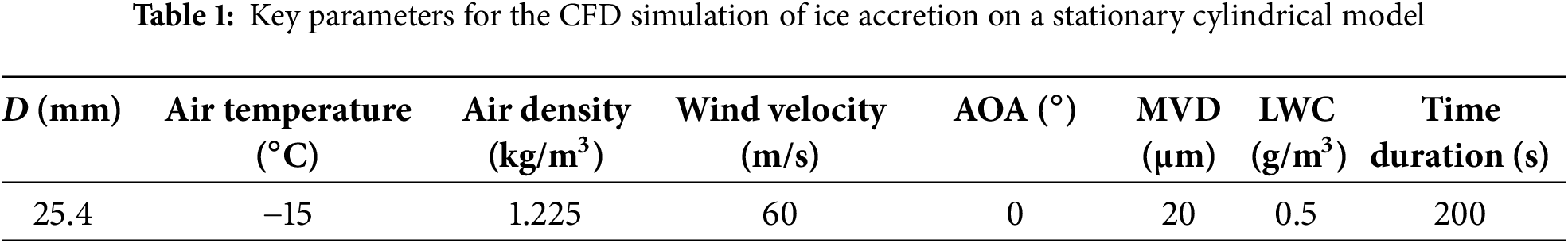

Figure 4: Comparison of the ice accretion on a cylinder between the numerical prediction and the experimental data: (a) Computational domain; and (b) Comparison results [58]
4.1.1 Geometry Model and Meshing
After validating the proposed numerical framework in the previous section, it is applied to simulate ice accretion on a flat plate. In this study, the geometry of the flat plate is defined with a width (B) of 0.4 m and a height (H) of 0.01 m, resulting in a width-to-height ratio of 40. This aspect ratio aligns with the definition of a flat plate in engineering practice. To minimize flow separation at the leading edge and ensure optimal flat plate characteristics, both the front and rear edges of the model are rounded with a 10 mm radius. The computational domain has dimensions of 15B by 10B, with a blockage ratio of 0.25%. Since FENSAP-ICE, the software used for simulations, requires 3D models, and to minimize the effect of spanwise dimensions on the results, the spanwise length is extended by the width of the flat plate, as suggested by Cao et al. [59]. The boundary conditions for the computational domain are as follows: the left side, along with the top and bottom boundaries, are defined as velocity inlets; the right side is set as a pressure outlet; the front and rear boundaries are treated as symmetry conditions; and the flat plate section is modeled with a fixed wall boundary. For mesh generation, ICEM CFD preprocessing software is used to ensure high-quality grids near the surface of the plate. A total of 50 layers are applied to refine the mesh, ensuring accuracy in the near-wall regions. To maintain y+ <1, the thickness of the first mesh layer is set to 0.01 mm, with a mesh growth rate of 1.05. Fig. 5 illustrates the geometry of the flat plate, along with the computational domain, mesh distribution, and boundary conditions.

Figure 5: Numerical model of the flat plate (mm): (a) Schematic of the flat plate; and (b) Computational domain and boundary conditions
4.1.2 Solution and Mesh Sensitivity
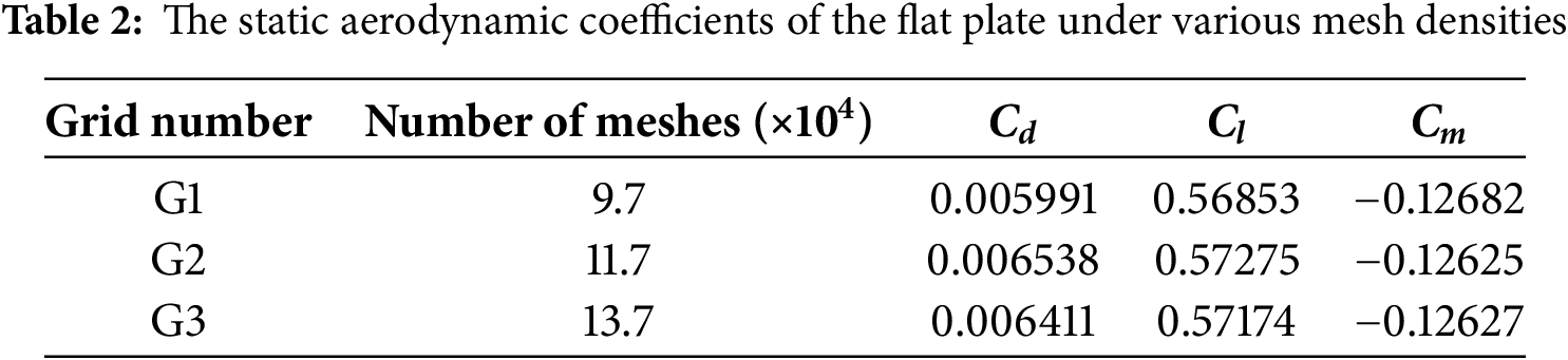
The numerical simulations of the airflow fields are conducted using the commercial CFD software ANSYS FLUENT 2022 R1. During the preprocessing phase, the fluid is modeled as an incompressible ideal gas to accurately simulate natural convection. The boundary conditions are defined as follows: the turbulent intensity for all velocity inlets and the pressure outlet is set to 0.5%, with a turbulent viscosity ratio of 2; the relative pressure at the pressure outlet is set to zero; and the walls are modeled as stationary, no-slip boundaries within the computational domain. Additionally, the wind speed and air temperature are adjusted according to the specific conditions for each scenario. In the solution phase, pressure-velocity coupling is achieved using the Coupled algorithm [45]. The convection and diffusion terms are discretized with a second-order upwind scheme, and a convergence criterion is set with a residual threshold of 10−6. The simulation is considered converged when all scaled residuals either stabilize or fall below the specified threshold. Moreover, mesh independence is verified to ensure an optimal balance between computational efficiency and accuracy. Three models with varying mesh densities are tested by changing the number of wall layers: 97,000, 117,000, and 137,000 elements. The thickness of the first mesh layer is consistently set to 0.01 mm across all models, with wall layer numbers set to 40, 50, and 60, respectively. For instance, with a wind speed of 20 m/s and a wind attack angle of 5°, the static aerodynamic coefficients (Cd, drag coefficient; Cl, lift coefficient; and Cm, lift moment coefficient) are used for comparison. The results for these models are summarized in Table 2. The analysis shows that the results for meshes G2 and G3 stabilize and exhibit strong consistency, indicating that mesh G2 provides the required accuracy. Therefore, to optimize computational resources without sacrificing precision, mesh G2 is selected for subsequent simulations.
This section explores the effects of key environmental factors, including air temperature, wind velocity, and the angle of attack (AOA), on ice accretion. Additionally, the influence of ice accretion on the static aerodynamic coefficients is examined.
4.2.1 Effect of Air Temperature on Ice Accretion
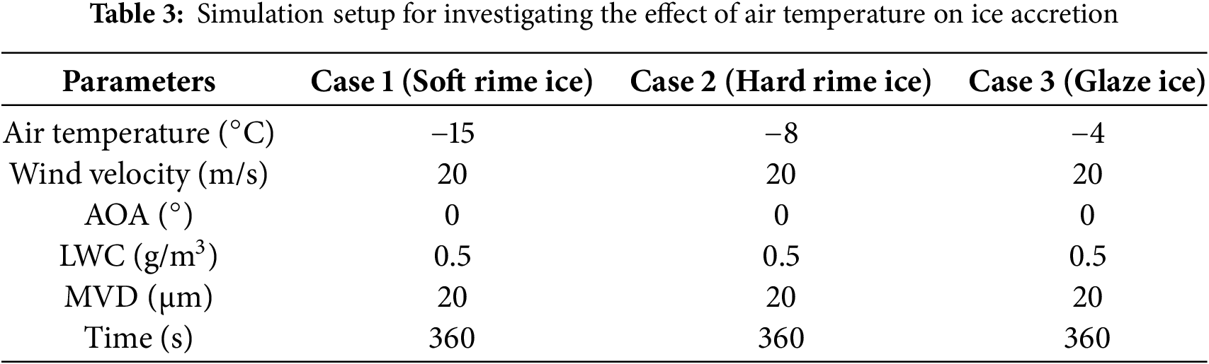
As discussed earlier, the relationship between icing types, wind speed, and temperature indicates that, at a constant wind speed, the icing type shifts from soft rime to hard rime as the temperature increases (Fig. 2). Once the temperature reaches a certain threshold, the icing type transitions to glaze. To better understand the impact of temperature on the morphology of ice accretion and to distinguish between these different types, three temperatures, i.e., −15°C, −8°C, and −4°C, are chosen to represent the conditions for soft rime, hard rime, and glaze ice, respectively. The wind speed is maintained at 20 m/s. First, the flow field around the flat plate is obtained through CFD simulations. The results are then imported into FENSAP-ICE, where parameters such as liquid water content, droplet diameter, and icing duration are set to calculate the ice accretion. The specific conditions used for the icing calculations are summarized in Table 3.
In this study, the “quasi-steady method” is utilized for the numerical simulation of ice accretion. According to preliminary calculations, a time step of 10 s is selected to enhance the simulation’s accuracy. This choice is based on a series of sensitivity analyses and trial simulations conducted using multiple time-step settings, guided by the experimental results reported in the validation study presented in Section 3 [58]. The comparison indicated that the 10-s step produced the closest agreement with the reference experimental data, thereby ensuring the reliability of the icing simulations. However, this choice also leads to a significant increase in computational time. To mitigate this issue and improve computational efficiency, the icing similarity law is applied [58]. This law provides a framework for determining the size and environmental conditions of a scaled model based on the dimensions and meteorological conditions of a reference model, ensuring that the icing results remain comparable. Initially developed to extend the capabilities of icing wind tunnels, the method is especially useful when experimental limitations, such as wind speed, liquid water content, or droplet diameter, restrict achievable conditions, or when full-scale testing is impractical due to test section size constraints. By applying the similarity law, the range of test conditions and model sizes can be effectively expanded within the existing experimental framework [58]. In this context, the icing similarity law also offers a practical approach to conserving computational resources and reducing simulation time.
Over the years, numerous studies have explored icing similarity, with several similarity criteria proposed by researchers [60], including the droplet inertia parameter (K), the collected water amount parameter (Ac), the leading-edge freezing coefficient (n0), and the Weber number (We). Based on these criteria, various methods have been developed to guide the selection of appropriate test parameters [61–63]. A particularly simple approach for scaling liquid water content and icing time involves maintaining a constant product of these two variables, while keeping all other conditions unchanged [63]. This approach ensures comparable ice accretion under different conditions by preserving the balance between water content and icing duration. For example, as shown in Table 3, an initial condition with a liquid water content of 0.5 g/m3 and an icing time of 360 s can be scaled to a liquid water content of 0.9 g/m3 and an icing time of 200 s, while maintaining all other parameters constant. This scaling method has been validated through numerical simulations, with the corresponding computational settings and results presented in Table 4 and Fig. 6. The results demonstrate that, under both the reference and scaled conditions, the simulated ice shape and thickness on the flat plate surface match closely, confirming the reliability and feasibility of the similarity approach. Consequently, for the subsequent simulations, the liquid water content and icing time are set to 0.9 g/m3 and 200 s, respectively, optimizing computational efficiency while ensuring accurate results. It is also important to note that in Table 4, the angle of attack (AOA) is set to 10°, where positive and negative values correspond to upward and downward flow directions, respectively, as shown in Fig. 6a. This convention for the sign of AOA will be consistently applied throughout the rest of the study.
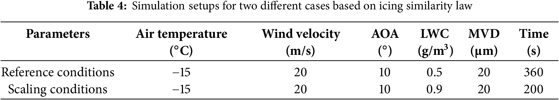


Figure 6: Comparison of the ice accretion between the reference and scaled conditions: (a) Definition of AOA; and (b) Comparison results (reference condition: t = 360 s, LWC = 0.5 g/m3; scaled condition: t = 200 s, LWC = 0.9 g/m3)
Fig. 7 illustrates the ice accretion patterns for soft rime, hard rime, and glaze ice on the flat plate under three distinct conditions. In these plots, the horizontal axis (x) and vertical axis (y) represent the positions along the width and height of the flat plate, respectively, as shown in Fig. 5a. This coordinate system is used consistently throughout all subsequent figures. The results indicate that for all three types of ice, the accretion is primarily concentrated at the leading edge of the plate, with ice thickness increasing linearly over time. Under rime conditions, the environmental temperature is low enough that water droplets freeze instantly upon contact with the plate surface. As a result, both soft rime and hard rime ice exhibit a smooth, streamlined growth pattern with consistent morphology and minimal change over time. In contrast, glaze ice forms under higher temperatures, which prevent the immediate release of latent heat during freezing. Consequently, droplets that impact the plate surface do not freeze completely but instead form a thin water film. This film moves toward the leading edge, where it eventually refreezes, creating protruding ice horns. Over time, the increasing number of impacting droplets leads to a rougher ice surface. Although glaze ice covers a larger area than rime ice under the same icing duration, the ice thickness in rime conditions is greater. Notably, hard rime results in the thickest ice layer among the three types, with the maximum thickness occurring at the leading edge. Specifically, the maximum ice thickness is 3.51 mm for soft rime, 3.26 mm for hard rime, and 1.92 mm for glaze ice, the latter being observed at the most prominent ice horn. These results indicate that higher temperatures result in thinner ice layers and more irregular glaze ice formations. The findings underscore the significant influence of temperature on the final ice accretion pattern, as it directly affects the heat transfer process when droplets impact the surface of the structure.

Figure 7: Ice accretion patterns for soft rime, hard rime, and glaze ice on the flat plate: (a) Case 1 (soft rime ice); (b) Case 2 (hard rime ice); and (c) Case 3 (glaze ice)
4.2.2 Effect of Wind Velocity and Angle of Attack (AOA) on Ice Accretion
In real-world conditions, both the incoming wind velocity and the angle of attack (AOA) can vary significantly, making it crucial to understand their impact on ice accretion. To demonstrate this, the effects of wind velocity and AOA on rime ice accretion are investigated. Specifically, a combination of four wind velocities (1, 5, 10, and 20 m/s) and five different AOA values (−10°, −5°, 0°, 5°, and 10°) are considered, as summarized in Table 5. All other parameters align with the soft rime icing conditions, i.e., the temperature is set to −15°C, the liquid water content is 0.9 g/m3, the droplet diameter is 20 μm, and the icing time is 200 s.
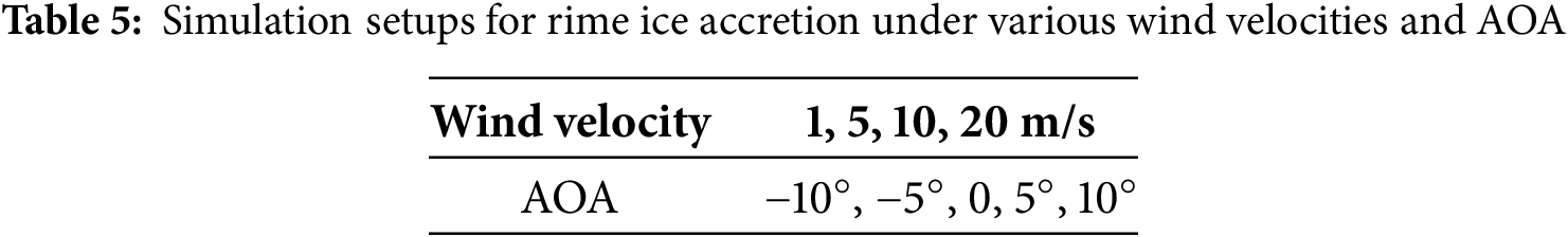
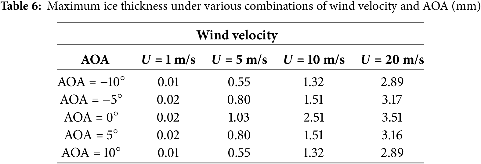
Fig. 8 shows the patterns of ice accretion on a flat plate under different wind speed conditions, with AOA of 0°, 5°, −5°, 10°, and −10°. The results reveal that as wind speed increases, water droplets are more likely to strike the leading edge of the plate. Specifically, for the same duration of icing, higher wind speeds result in a greater number of droplets impacting the surface. Additionally, increased wind speed helps carry away more of the latent heat released during the freezing process, which accelerates the ice accretion and leads to an increase in both the thickness and extent of the ice layer. Despite these changes, wind speed does not significantly affect the overall shape of the ice growth. As an example, when the wind speed increases from U = 1 to 5 m/s, 10, and 20 m/s at a 0° angle of attack, the ice thickness on the flat plate rapidly increases from 0.02 to 1.03 mm, 2.51, and 3.51 mm, respectively. This highlights the significant impact of wind speed on the ice thickness. Table 6 presents the maximum ice thickness under various combinations of wind speed and AOA. It is also noted that for AOAs of equal magnitude but opposite sign, the maximum ice thickness values are identical, owing to the symmetry of the flow and ice accretion patterns about the horizontal axis. Furthermore, as shown in Fig. 8, increasing wind speed does not change the overall shape of the ice layer. Notably, when the wind speed is 1 m/s, ice accretion on the plate is minimal under the given environmental conditions. This is due to the insufficient number of droplets impacting the plate at low wind speeds, making it more difficult for the droplets to reach the surface. Therefore, the analysis confirms that wind speed is a crucial factor in determining whether ice will accumulate on the flat plate. If the wind speed is too low, noticeable icing may take longer to develop.
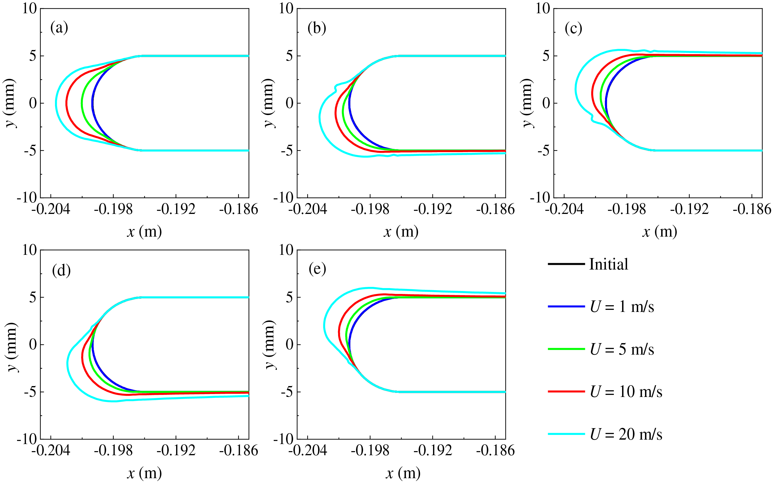
Figure 8: Effect of wind velocity on ice accretion under various AOAs: (a) AOA = 0°; (b) AOA = 5°; (c) AOA = −5°; (d) AOA = 10°; and (e) AOA = −10°
To further investigate the effect of AOA on ice accretion patterns on the flat plate, the ice accumulation patterns at various AOAs are compared, as shown in Fig. 9. As shown in Fig. 9, increasing the AOA results in an increased impact limit on the pressure side and a decreased impact limit on the suction side. This shift leads to a migration of the ice accretion area towards the pressure side of the plate. In other words, the normal direction at the point of maximum ice thickness aligns closely with the direction of the AOA, indicating that the AOA plays a key role in determining the location of maximum ice accumulation. The movement of the ice accretion zone towards the pressure side also implies that the ice accretion shifts from the leading edge of the plate towards the upper (or lower, depending on the direction of the incoming wind and AOA) surface. This results in an increase in the ice coverage on the surface of the plate. However, due to the relatively short icing time used in these calculations, the ice thickness and the amount of ice on the upper (or lower) surfaces are negligible. If a longer icing time were considered, more significant ice accumulation might occur on these surfaces. Moreover, under conditions of both positive and negative attack angles (with the same absolute value but opposite signs), the ice accretion patterns on the flat plate are symmetrically distributed with respect to the horizontal axis (the axis of symmetry).
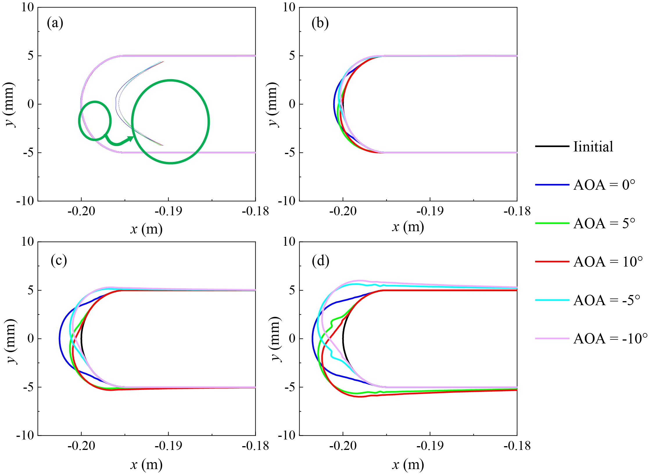
Figure 9: Ice accretion patterns at various AOAs: (a) U = 1 m/s; (b) U = 5 m/s; (c) U = 10 m/s; and (d) U = 20 m/s
4.2.3 Effect of Soft Rime Ice on Aerodynamic Coefficients
The accumulation of ice on the surface of the flat plate changes its shape, which, in turn, influences the surrounding flow field and affects the aerodynamic coefficients. These coefficients are crucial for evaluating the wind resistance performance of structures. For example, aerodynamic coefficients are key in flutter analysis, as they form the foundation for identifying flutter derivatives. In the field of bridge wind engineering, these coefficients are used to calculate the drag, lift, and moment forces acting on the bridge structure, allowing for further analysis of stress and displacement under steady wind loads, as well as evaluations of static wind stability. Therefore, studying the variations in aerodynamic coefficients before and after ice accretion is essential to fully understanding the impact of icing on the overall performance of the structure.
Fig. 10 presents the aerodynamic coefficients of the flat plate before and after the formation of soft rime ice (refer to Case 1 in Table 3). The results show that, under the selected soft rime icing conditions, the shape of the plate’s leading edge does not change significantly, leading to relatively similar aerodynamic coefficients before and after icing. For the drag coefficient, a slight decrease is observed after icing. This is attributed to the smoothing and flattening of the leading edge, as seen in the ice distribution pattern in Fig. 7a. Notably, a negative drag coefficient is observed at an angle of attack of −5°. This anomaly occurs because, at this angle, the higher wind speed causes the ice formation at the plate’s leading edge to develop a small ice horn (as shown in Fig. 8), which alters the flow field and results in a negative drag coefficient. Conversely, both the lift coefficient and the lift moment coefficient show a slight increase, with both coefficients rising as the angle of attack increases, both before and after icing.

Figure 10: Static aerodynamic coefficients of the flat plate before and after ice accretion: (a) Cd; (b) Cl; and (c) Cm
This study develops and applies an integrated CFD–FENSAP-ICE numerical framework to simulate ice accretion on flat plates, with emphasis on quantifying the influence of environmental parameters and assessing aerodynamic impacts. The research primarily focuses on investigating ice formation patterns and thickness under different temperatures, analyzing the effects of varying wind speeds and angles of attack (AOA) on soft rime ice accretion, and examining the aerodynamic consequences of rime ice. The main conclusions are as follows:
(1) The ice thickness on the flat plate increases approximately linearly over time. In the case of rime ice, the relatively low environmental temperature causes water droplets to freeze instantly upon impact, leading to streamlined growth. In contrast, glaze ice forms at higher temperatures, preventing immediate freezing. Instead, the impacting droplets create a thin water film that flows towards the leading edge and refreezes, forming protruding ice horns. Under identical conditions, rime ice consistently produces thicker ice layers than glaze ice, with the maximum thickness occurring at the leading edge, whereas glaze ice exhibits its greatest thickness at the horn tips. These observations confirm the dominant role of temperature in controlling ice morphology via heat transfer processes.
(2) Increasing wind speed results in more droplets striking the surface and enhances latent heat removal, thereby accelerating the ice accretion rate and increasing both thickness and coverage. At very low wind speeds (e.g., 1 m/s), droplet impingement is minimal and ice accumulation is negligible under the tested conditions, indicating a threshold wind speed for noticeable accretion.
(3) Increasing AOA expands the impingement region on the pressure side while reducing it on the suction side, shifting the icing zone toward the pressure surface. For AOAs of equal magnitude but opposite sign, the ice accretion patterns are symmetric about the horizontal axis, yielding identical maximum ice thickness values.
(4) Ice accretion modifies the leading-edge geometry, making it smoother and more streamlined. This slightly reduces the drag coefficient compared with the pre-icing state. At –5° AOA and higher wind speeds, localized horn formation alters the flow field, leading to a negative drag coefficient in that case. The lift and moment coefficients show slight increases, with both rising as AOA increases, before and after icing.
This study investigates ice accretion on flat plates and its impact on structural performance, providing baseline insights and feasibility evidence for subsequent research. Its limitation lies in focusing on basic icing scenarios under specific computational conditions. Future work will extend the framework toward application relevant systems by (i) moving from flat plates to representative geometries in aircraft (airfoils/wings), wind turbines (rotating blades), and bridges (cables/box girders); (ii) incorporating fully time dependent icing to capture unsteady accretion and active/operational de icing scenarios, with dynamic mesh updates to resolve ice growth and shedding; (iii) assessing alternative turbulence models and performing targeted sensitivity/uncertainty analyses; and (iv) calibrating and validating the predictions against wind tunnel or field measurements under similarity law consistent conditions. These steps will enhance both the generalizability and practical impact of the framework.
Acknowledgement: None.
Funding Statement: This work is supported by the National Natural Science Foundation of China (52278532) and Sichuan Science and Technology Program (2024NSFSC0153). These supports are greatly appreciated.
Author Contributions: Jin Zhu: Conceptualization; Supervision; Funding acquisition; Writing—review & editing. Yanxin Xu: Formal analysis; Investigation; Methodology; Writing—original draft. All authors reviewed the results and approved the final version of the manuscript.
Availability of Data and Materials: All data, models, or codes that support the findings of this study are available upon reasonable request.
Ethics Approval: Not applicable.
Conflicts of Interest: The authors declare no conflicts of interest to report regarding the present study.
Nomenclature/Abbreviations
| List of Symbols | |
| xi,ui | Coordinates and velocity tensors of the i-axis in a coordinate system |
| xj,uj | Coordinates and velocity tensors of the j-axis in a coordinate system |
| t | Time |
| ρa | Air density |
| pa | Air pressure |
| μa | Air dynamic viscosity |
| fi | Body force per unit volume in xi direction |
| Pk,Pω | Production term |
| F1, F2 | Blending function |
| μt | Turbulent eddy viscosity |
| y | Distance from the field point to the nearest wall |
| τij | Reynolds stress tensor |
| Ω | Vorticity magnitude |
| α | Droplet volume fraction |
| Velocity vector of air in the flow field | |
| Velocity vector of droplet in the flow field | |
| Gravitational acceleration | |
| Red | Droplet Reynolds number |
| K | Droplet inertial parameter |
| Fr | Froude number |
| CD | Droplet drag coefficient |
| ρd | Droplet density |
| d | Droplet diameter |
| Freestream velocity | |
| L∞ | Characteristic length |
| f | Water film |
| ρf | Water film density |
| hf | Water film height |
| Water film velocity vector | |
| β | Local collection efficiency |
| Mass flux of evaporation | |
| Mass flux of ice accretion | |
| cf | Heat capacity of water film |
| cice | Heat capacity of ice |
| Freestream temperature (°C) | |
| Equilibrium temperature (°C) | |
| T∞ | Freestream temperature (K) |
| T | Equilibrium temperature (K) |
| Levap | Latent heat of evaporation |
| Lsubl | Latent heat of sublimation |
| Lfus | Latent heat of fusion |
| ε | Solid emissivity coefficient |
| σ | Boltzmann constant |
| Convective heat flux | |
| ρice | Ice density |
| Δt | Icing time increment |
| Icing velocity vector | |
| Δhice | Icing surface displacement |
| Surface normal vector | |
| D | Cylindrical diameter |
| Cd | Drag coefficient |
| Cl | Lift coefficient |
| Cm | Lift moment coefficient |
| Ta | Air temperature |
| U | Wind velocity |
| Ac | Parameter of water volume accumulation |
| n0 | Leading edge freezing fraction |
| We | Weber number |
| List of Abbreviations | |
| CFD | Computational fluid dynamics |
| AOA | Angle of attack |
| LWC | Liquid water content |
| MVD | Median volume droplet diameter |
| IoT | Internet of Things |
| SST | Shear-Stress Transport |
References
1. Xie RH, Liao CH, Luo X, Guo HF, Huang ZQ, Peng WY. Research on road surface temperature characteristics and road ice warning model of ordinary highways in winter in Hunan province, central China. Front Earth Sci. 2023;11:1251635. doi:10.3389/feart.2023.1251635. [Google Scholar] [CrossRef]
2. Kamenchukov AV, Tyan VD, Voinash SA, Ariko SY, Teterina IA, Sokolova VA, et al. Modeling heat transfer processes in heating systems for surface of highways. J Phys Conf Ser. 2020;1679(4):042045. doi:10.1088/1742-6596/1679/4/042045. [Google Scholar] [CrossRef]
3. Cao YH, Tan WY, Wu ZL. Aircraft icing: an ongoing threat to aviation safety. Aerosp Sci Technol. 2018;75(5):353–85. doi:10.1016/j.ast.2017.12.028. [Google Scholar] [CrossRef]
4. Yirtici O, Tuncer IH, Ozgen S. Ice accretion prediction on wind turbines and consequent power losses. J Phys Conf Ser. 2016;753(2):022022. doi:10.1088/1742-6596/753/2/022022. [Google Scholar] [CrossRef]
5. Shu LC, Liang J, Hu Q, Jiang XL, Ren XK, Qiu G. Study on small wind turbine icing and its performance. Cold Reg Sci Technol. 2017;134(1):11–9. doi:10.1016/j.coldregions.2016.11.004. [Google Scholar] [CrossRef]
6. Laakso T, Holttinen H, Ronsten G, Tallhaug L, Horbaty R, Baring-Gould I, et al. State-of-the-art of wind energy in cold climates. IEA Annex XIX. 2003;24:53. [Google Scholar]
7. Parent O, Ilinca A. Anti-icing and de-icing techniques for wind turbines: critical review. Cold Reg Sci Technol. 2011;65(1):88–96. doi:10.1016/j.coldregions.2010.01.005. [Google Scholar] [CrossRef]
8. Lamraoui F, Fortin G, Benoit R, Perron J, Masson C. Atmospheric icing impact on wind turbine production. Cold Reg Sci Technol. 2014;100:36–49. doi:10.1016/j.coldregions.2013.12.008. [Google Scholar] [CrossRef]
9. Cao YH, Ma C, Zhang Q, Sheridan J. Numerical simulation of ice accretions on an aircraft wing. Aerosp Sci Technol. 2012;23(1):296–304. doi:10.1016/j.ast.2011.08.004. [Google Scholar] [CrossRef]
10. Cao YH, Huang JS, Yin J. Numerical simulation of three-dimensional ice accretion on an aircraft wing. Int J Heat Mass Transf. 2016;92(1):34–54. doi:10.1016/j.ijheatmasstransfer.2015.08.027. [Google Scholar] [CrossRef]
11. Feng YP, Zhang B, Chen B. Lift/Drag characteristics of different ice accretion airfoil. IOP Conf Ser Mater Sci Eng. 2019;612(2):022008. [Google Scholar]
12. Lian WL, Zhao L, Xuan YM, Shen JD. A modified spongy icing model considering the effect of droplets retention on the ice accretion process. Appl Therm Eng. 2018;134(8):54–61. doi:10.1016/j.applthermaleng.2018.01.107. [Google Scholar] [CrossRef]
13. Dai H, Zhu CL, Zhao HY, Liu SY. A new ice accretion model for aircraft icing based on phase-field method. Appl Sci. 2021;11(12):5693. doi:10.3390/app11125693. [Google Scholar] [CrossRef]
14. Zheng CY, Jin ZY, Dong QT, Yang ZG. Numerical investigation of the influences of ridge ice parameters on lift and drag coefficients of airfoils through design of experiments. Adv Mech Eng. 2024;16(1):1–12. doi:10.1177/16878132231226056. [Google Scholar] [CrossRef]
15. Bhatia D, al Wahaibi AYS. A numerical investigation into the impact of icing on the aerodynamic performance of aerofoils. IOP Conf Ser Mater Sci Eng. 2019. 2020;831(1):012007. [Google Scholar]
16. Liu Y, Hu H. An experimental investigation on the unsteady heat transfer process over an ice accreting airfoil surface. Int J Heat Mass Transf. 2018;122(5):707–18. doi:10.1016/j.ijheatmasstransfer.2018.02.023. [Google Scholar] [CrossRef]
17. Wu J, Xu QY, Wu F, Xia QZ, Xu QN. The icing characteristic of stage 35 compressor blades and its impact on aerodynamic performance. Aeros Sci Technol. 2024;150(7):109222. doi:10.1016/j.ast.2024.109222. [Google Scholar] [CrossRef]
18. Nogi K, Imamura T. Numerical simulation of rime ice accretion on airfoil using rigid sphere model. Comput Fluids. 2024;275(6):106244. doi:10.1016/j.compfluid.2024.106244. [Google Scholar] [CrossRef]
19. Cao YH, Xin M. Numerical simulation of ice accretion in supercooled large droplet conditions. Sci China Technol Sc. 2019;62(7):1191–201. doi:10.1007/s11431-017-9265-3. [Google Scholar] [CrossRef]
20. Shad A, Sherif SA. Quasi-steady simulation of glaze ice accretion and heat transfer in the supercooled large droplet regime in atmospheric turbulent air flow. ASME J Heat Mass Transf. 2023;145(5):053001. doi:10.1115/1.4056069. [Google Scholar] [CrossRef]
21. Farghaly MB, Aldabesh A, Aljohani BS, Saleh AEL, Mohamed ET, Alareqi FS, et al. Studying the effect of geometric parameters of anti-icing system on the performance characteristics of airplane wing: computational analysis. Case Stud Therm Eng. 2025;73(2):106733. doi:10.1016/j.csite.2025.106733. [Google Scholar] [CrossRef]
22. Abdelghany ES, Farghaly MB, Almalki MM, Sarhan HH, Essa MEM. Machine learning and IoT trends for intelligent prediction of aircraft wing anti-icing system temperature. Aerospace. 2023;10(8):676. doi:10.3390/aerospace10080676. [Google Scholar] [CrossRef]
23. Song Y, Liu R, Li S, Kang Z, Zhang F. Peridynamics modeling and simulation of coupled thermomechanical removal of ice from frozen structures. Meccanica. 2019;55(4):961–76. doi:10.1007/s11012-019-01106-z. [Google Scholar] [CrossRef]
24. Song Y, Li S, Zhang S. Peridynamic modeling and simulation of thermo-mechanical de-icing process with modified ice failure criterion. Def Technol. 2020;17(1):15–35. doi:10.1016/j.dt.2020.04.001. [Google Scholar] [CrossRef]
25. Li Y, Sun C, Jiang Y, Yi X, Xu Z, Guo WF. Temperature effect on icing distribution near blade tip of large-scale horizontal-axis wind turbine by numerical simulation. Adv Mech Eng. 2018;10(11):1–13. doi:10.1177/1687814018812247. [Google Scholar] [CrossRef]
26. Zhang TG, Zhou XY, Liu ZB. Numerical simulation of rime ice accretion on a three-dimensional wind turbine blade using a Lagrangian approach. Front Struct Civ Eng. 2024;17(12):1895–906. doi:10.1007/s11709-023-0971-0. [Google Scholar] [CrossRef]
27. Guan X, Li MY, Wu SW, Xie YQ, Sun YP. Influence of surface ice roughness on the aerodynamic performance of wind turbines. Fluid Dyn Mater Proc. 2024;20(9):2029–43. doi:10.32604/fdmp.2024.049499. [Google Scholar] [CrossRef]
28. Dai YJ, Xie FZ, Li BH, Wang C, Shi KJ. Effect of blade tips ice on vibration performance of wind turbines. Energy Rep. 2023;9(7):622–9. doi:10.1016/j.egyr.2022.12.092. [Google Scholar] [CrossRef]
29. Wang ZZ, Zhu CL. Numerical simulation for in-cloud icing of three-dimensional wind turbine blades. Simul-T Soc Mod Sim. 2018;94(1):31–41. doi:10.1177/0037549717712039. [Google Scholar] [CrossRef]
30. Manatbayev R, Baizhuma Z, Bolegenova S, Georgiev A. Numerical simulations on static Vertical Axis Wind Turbine blade icing. Renew Energ. 2021;170:997–1007. doi:10.1016/j.renene.2021.02.023. [Google Scholar] [CrossRef]
31. Chen JQ, Wu QL, Wang H, Quan ZQ, Dan HC. Modeling and analysis of ice condensation on bridge deck pavement surface based on heat transfer theory and finite element method. Appl Therm Eng. 2024;241(4):122344. doi:10.1016/j.applthermaleng.2024.122344. [Google Scholar] [CrossRef]
32. Yang EH, Yang QL, Li J, Zhang HP, Di HB, Qiu YJ. Establishment of icing prediction model of asphalt pavement based on support vector regression algorithm and Bayesian optimization. Constr Build Mater. 2022;351(6):128955. doi:10.1016/j.conbuildmat.2022.128955. [Google Scholar] [CrossRef]
33. Li WT, Geng ZY, Xiao HL, Pei YY, Yang K. An experimental study on ice accretion under bridge cable in different conditions. Appl Sci. 2023;13(6):3963. doi:10.3390/app13063963. [Google Scholar] [CrossRef]
34. Xu FY, Yu HY. Effect of ice accretion on the aerodynamic responses of a pipeline suspension bridge. J Bridge Eng. 2020;25(10):04020091. doi:10.1061/(asce)be.1943-5592.0001625. [Google Scholar] [CrossRef]
35. Yu HY, Xu FY, Zhang MJ, Zhou AQ. Experimental investigation on glaze ice accretion and its influence on aerodynamic characteristics of pipeline suspension bridges. Appl Sci. 2020;10(20):7167. doi:10.3390/app10207167. [Google Scholar] [CrossRef]
36. Yu HY, Zhang MJ, Xu FY. Effect of ice accretion on aerodynamic characteristics of pipeline suspension bridges. Structures. 2022;46(9):1851–62. doi:10.1016/j.istruc.2022.11.016. [Google Scholar] [CrossRef]
37. Górski P, Tatara M, Pospíšil S, Kuznetsov S. Model investigations of the aerodynamic coefficients of iced cables in cable-stayed bridges. Tech Trans. 2019;12(8):115–27. doi:10.4467/2353737xct.19.083.10862. [Google Scholar] [CrossRef]
38. Tang M, Cao YH, Zhong G. Numerical simulation of ice accretion on helicopter rotor blades with trailing edge flap. Aircr Eng Aerosp Tec. 2024;96(9):1165–71. doi:10.1108/aeat-02-2024-0027. [Google Scholar] [CrossRef]
39. Fu ZG, Feng WJ, Wang ZJ, Liu B. Three-dimensional numerical simulation of ice accretion on rotating components of engine entry. Trans Nanjing Univ Aeronaut Astronaut. 2023;40(6):663–77. [Google Scholar]
40. Zhou C, Yin JQ. Numerical analysis of glaze ice accretion on cables by considering the effects of typical in-plane vibrations. J Fluids Struct. 2024;131(1776):104229. doi:10.1016/j.jfluidstructs.2024.104229. [Google Scholar] [CrossRef]
41. Liu ZY, Hu YY, Jiang XL, Wu Y, Chi MC, Han FY, et al. Three-dimensional numerical simulation of rime ice accumulation on silicone rubber insulator and its experimental verification in the natural environment. Electr Pow Syst Res. 2022;213:108713. doi:10.1016/j.epsr.2022.108713. [Google Scholar] [CrossRef]
42. Wu B, Wang Q, Liao HL, Li ZG. Flutter mechanism of thin flat plates under different attack angles. J Vib Eng. 2020;33(4):667–78. (In Chinese). [Google Scholar]
43. Fortin G, Perron J. Wind turbine icing and de-icing. In: Proceedings of the 47th AIAA Aerospace Sciences Meeting including the New Horizons Forum and Aerospace Exposition; 2009 Jan 5–8; Orlando, FL, USA. [Google Scholar]
44. ISO Copyright Office. Atmospheric icing of structures (ISO 12494). 2017 [Internet]. [cited 2025 Aug 28]. Available from: https://www.iso.org/contents/data/standard/07/24/72443.html. [Google Scholar]
45. Zhang ZR, Zhang XW, Yan JH. Manifold method coupled velocity and pressure for Navier-Stokes equations and direct numerical solution of unsteady incompressible viscous flow. Comput Fluids. 2010;39(8):1353–65. doi:10.1016/j.compfluid.2010.04.005. [Google Scholar] [CrossRef]
46. Menter FR. Improved two-equation k-omega turbulence models for aerodynamic flows. NASA Tech Rep Server. 1992;93:22809. [Google Scholar]
47. Menter FR. Zonal two equation κ-ω turbulence models for aerodynamic flows. In: Proceedings of the 24rd Fluid Dynamics Conference; 1993 Jul 6–9; Orlando, FL, USA. [Google Scholar]
48. Yassin K, Hassan K, Bernhard S, Thomas K, Joachim P. Numerical simulation of roughness effects of ice accretion on wind turbine airfoils. Energies. 2022;15(21):8145. doi:10.3390/en15218145. [Google Scholar] [CrossRef]
49. Philipbar BM, Waters JJ, Carrington DB. A finite element menter shear stress turbulence transport model. Numer Heat Tr A-Appl. 2020;77(12):981–97. doi:10.1080/10407782.2020.1746155. [Google Scholar] [CrossRef]
50. Zhu CL, Zhu CX. Aircraft icing and its protection. Beijing, China: Science Press; 2015. (In Chinese). [Google Scholar]
51. Debenedetti PG, Stanley HE. Supercooled and glassy water. J Phys-Condens Mat. 2003;15(45):R1669. doi:10.1088/0953-8984/15/45/r01. [Google Scholar] [CrossRef]
52. Wang C, Chang S, Wu H. Lagrangian approach for simulating supercooled large droplets’ impingement effect. J Aircr. 2015;52(2):524–37. doi:10.2514/1.c032765. [Google Scholar] [CrossRef]
53. Wirogo S, Srirambhatla S. An Eulerian method to calculate the collection efficiency on two and three dimensional bodies. In: Proceedings of the 41st Aerospace Sciences Meeting and Exhibit; 2003 Jan 6–9; Reno, NV, USA. [Google Scholar]
54. Bourgault Y, Habashi WG, Dompierre J, Baruzzi GS. A finite element method study of Eulerian droplets impingement models. Int J Numer Meth Fluids. 1999;29(4):429–49 doi:10.1002/(sici)1097-0363(19990228)29:4<429::aid-fld795>3.0.co;2-f. [Google Scholar] [CrossRef]
55. Bourgault Y, Habashi WG, Dompierre J, Boutanios Z, Di Bartolomeo W. An Eulerian approach to supercooled droplets impingement calculations. In: Proceedings of the AIAA 35th Aerospace Sciences Meeting and Exhibit; 1997 Jan 6–9; Reno, NV, USA. [Google Scholar]
56. Bourgault Y, Beaugendre H, Habashi WG. Development of a shallow-water icing model in FENSAP-ICE. J Aircr. 2000;37(4):640–6 doi:10.2514/2.2646. [Google Scholar] [CrossRef]
57. Bourgault Y, Boutanios Z, Habashi WG. Three-dimensional Eulerian approach to droplet impingement simulation using FENSAP-ICE, part 1: model, algorithm, and validation. J Aircr. 2000;37(1):95–103 doi:10.2514/2.2566. [Google Scholar] [CrossRef]
58. Meng FX, Chen WJ, Liang QS, Zhang DL. Experiment on cylinder icing in injection driven icing wind tunnel. J Aerosp Pow. 2013;28(7):1467–74. (In Chinese). [Google Scholar]
59. Cao SY, Zhou Q, Zhou ZY. Velocity shear flow over rectangular cylinders with different side ratios. Comput Fluids. 2014;96:35–46 doi:10.1016/j.compfluid.2014.03.002. [Google Scholar] [CrossRef]
60. Kind RJ, Oleskiw MM. Experimental assessment of a water-film-thickness Weber number for scaling of glaze icing. In: Proceedings of the 39th AIAA Aerospace Sciences Meeting and Exhibit; 2001 Jan 8–11; Reno, NV, USA. [Google Scholar]
61. Ingelman-Sundberg M, Trunov O, Ivaniko A. Methods for prediction of the influence of ice on aircraft flying characteristics. Norrkoping, Sweden: Swedish Soviet Working Group on Flight Safety; 1977. Report No. JR1. [Google Scholar]
62. Anderson DN. Rime-, mixed-and glaze-ice evaluations of three scaling laws. In: Proceedings of the AIAA 32nd Aerospace Sciences Meeting and Exhibit; 1994 Jan 10–13; Reno, NV, USA. [Google Scholar]
63. Anderson DN, Ruff GA. Scaling methods for simulating aircraft in-flight icing encounters. In: Proceedings of the International Symposium on Scale Modeling; 1997 Jun 23–27; Lexington, KY, USA. [Google Scholar]
Cite This Article
 Copyright © 2025 The Author(s). Published by Tech Science Press.
This work is licensed under a Creative Commons Attribution 4.0 International License , which permits unrestricted use, distribution, and reproduction in any medium, provided the original work is properly cited.
 Downloads
 Citation Tools