Risk Indicator Identification for Coronary Heart Disease via Multi-Angle Integrated Measurements and Sequential Backward Selection

1  Introduction

According to the 2020 China Cardiovascular Health and Disease Report, the number of deaths from cardiovascular diseases in China has been increasing year-on-year over the past decade, especially in rural areas, where the number of deaths had surpassed those in urban areas by 2016. Among them, Coronary Heart Disease (CHD) is a kind of cardiovascular disease with high incidence, and the possibility of cure is low [1–3]. If patients with CHD can be diagnosed at an early stage of the disease and given effective prevention and treatment, the goal of aggressive treatment can be achieved, thereby reducing the risk of developing the disease and saving medical costs. As the incidence of CHD increases year by year, a single clinical treatment can no longer meet current needs. Establishing an accurate and effective risk assessment index system for CHD and early identification and intervention of important risk factors is urgently needed.

Globally, cardiovascular diseases (CVDs) remain the leading cause of mortality, accounting for approximately 32% of all deaths worldwide according to the World Health Organization (WHO). Among these, coronary heart disease (CHD) is the most prevalent, with an estimated 9.14 million deaths annually. The Global Burden of Disease (GBD) study indicates that CHD incidence has risen by 41% since 1990, underscoring its escalating threat to public health across both developed and developing nations. While China faces a particularly sharp increase in CHD prevalence—especially in rural areas—this trend is part of a broader global challenge [4]. Therefore, developing robust risk prediction models that are globally applicable yet sensitive to regional variations is of paramount importance.

The study of risk factors affecting CHD has significant social and economic value for the early identification and intervention of CHD. The reduction of the dimensionality of the CHD dataset through feature selection can simplify the dataset to the greatest extent, provided that the accuracy of the prediction results is ensured and the risk factors that have a greater impact on the risk of CHD are obtained. Effective feature selection is crucial not only for reducing dimensionality and computational cost but also for enhancing model interpretability and prediction accuracy. By eliminating irrelevant and redundant features, we can mitigate overfitting, improve generalization, and uncover the most clinically relevant risk factors [5]. Moreover, interpretable feature subsets allow clinicians to understand and trust model predictions, facilitating their integration into medical decision-making [6,7]. Thus, the integration of robust feature selection methods is essential for developing reliable and transparent CHD risk prediction models.

Based on the relationship with the learning algorithm after feature selection, it can be divided into Filter, Wrapper and Embedded [1]. Since individual feature selection methods have some limitations, it is easy to measure the importance of features only from a certain perspective, and the selected subset of features may not be optimal. At the same time, most hybrid feature selection methods are divided into two stages. In the Filter stage, only the characteristics of the data are considered for research, and in the Wrapper or Embedded stage, the classification performance of machine learning algorithm is used to measure the degree of importance, which fails to fully integrate data and algorithm for feature selection. In addition, the feature subsets obtained by most of the existing feature selection methods cannot effectively explain the prediction results of the model, and are not statistically explanatory. Based on the above questions, in this paper we start from the risk factors for coronary heart disease and aim at data on various physical indicators for different populations: Firstly, the importance degree of features is measured from multiple angles based on data and algorithm level, respectively, and a set of feature importance scores is obtained. Then, the score is sorted in descending order and the feature subset is screened with the accuracy of LightGBM model as the evaluation index according to the principle of backward sequence screening. Finally, the risk assessment index system of coronary heart disease is constructed based on the selected feature subset, and the risk of coronary heart disease is predicted.

Based on the above motivations, this study is guided by the following research hypothesis:

H: A feature selection framework that integrates measurements from multiple perspectives (data-level and algorithm-level) with a sequential backward selection strategy will identify a more predictive and interpretable subset of risk indicators for coronary heart disease, leading to a risk prediction model with higher accuracy and better clinical utility compared to models using single-perspective feature selection methods.

To test this hypothesis, we aim to address the following research questions:

RQ1: Can a multi-angle integrated measurement approach effectively balance relevance, redundancy, and interpretability when evaluating feature importance for CHD risk prediction?

RQ2: Does the proposed SBS-based selection strategy successfully identify a compact yet highly predictive feature subset?

RQ3: Does the resulting model, built upon the selected features, achieve superior predictive performance while maintaining statistical interpretability?

In summary, this paper proposes a system-building approach for CHD risk assessment indicators based on multi-angle integrated measurements and SBS to identify important risk indicators for CHD and conduct early intervention to provide reliable data support for coronary heart disease risk prediction. The main contribution of the present study is as follows.

(1) This paper presents a method to calculate the characteristic importance of coronary heart disease risk factors based on multi-angle integrated measurements. At the data level, the mRMR algorithm is chosen to fully account for correlations and redundancies in the dataset. At the algorithm level, random forest algorithm is selected as the classification model, based on SHAP-RF and ARFS-RF, the importance of each risk feature is comprehensively calculated from the two perspectives of the interpretation degree of each feature in the classification algorithm to the results and the statistical interpretability of the classification algorithm. It provides a comprehensive multi-angle measure of feature importance.

(2) A CHD risk factor identification method based on multi-angle integrated measurements and SBS is proposed to construct a risk index system for coronary heart disease. In the multi-angle integrated measurements stage, three methods are used to calculate the feature importance, and the final feature importance score is taken as the modulus length of the three-dimensional vector. In the SBS stage, the features with the lowest feature importance scores are successively removed and the best feature subset is screened based on the classification accuracy of the LightGBM model. This method fully integrates the strengths and weaknesses at the data and algorithm level, reduces the probability of feature preferences, and the selected feature subset can effectively explain the model prediction results, which is statistically interpretable and can avoid the limitation of artificially setting threshold values for feature selection.

The rest of this paper is set as follows. Section 2 provides the literature review. Section 3 is devoted to data preparation and descriptive statistical analysis. The CHD dataset from the Kaggle data site is selected as the study subject, and the missing values are filled in to establish data equalization based on the features of the dataset itself. Moreover, a descriptive statistical analysis is performed on the data distribution of each feature and the relationship between each feature and the disease situation. Section 4 gives the basic idea of CHD risk factor identification, details the construction process of the CHD risk assessment indicator system based on multi-angle integrated measurements and SBS, and performs an empirical analysis based on the proposed method. Through a comparative analysis, the results show that this method can achieve higher prediction accuracy and screen a minimum number of feature subsets. Section 5 concludes the paper with an outlook on future work.

2  Literature Review

The causes of CHD are complex, many risk factors may induce CHD, and the onset of CHD is a long-term process, so it is very important to identify the risk of CHD in advance and carry out targeted treatment. Some researchers integrated medical technology and Machine Learning (ML) techniques to effectively reduce the rate of misdiagnosis, improve the efficiency of medical diagnosis, and effectively promote the development of medicine. Weng et al. [2] used four ML algorithms to predict the risk of cardiovascular diseases, which are as follows, Random Forest (RF), Logistic, Gradient Boosting (GB) and Artificial Neural Network (ANN) algorithms were compared with the prediction methods in the guidelines of the American College of Cardiology. It was found that the four ML algorithms used were better in Area Under Curve (AUC) values, specificity, sensitivity and other aspects. This suggests that ML algorithms can more accurately predict possible disease samples and avoid unnecessary treatment for low-risk individuals. Based on descriptive analysis, Xu [3] constructed Fine and Gray models and Logistic regression models, respectively, to predict the risk of CHD, providing simple and efficient tools for the early prediction of CHD. Wang et al. [8] proposed a cloud-random forest model (C-RF) for the risk assessment of CHD. The proposed method performs well on a variety of categorical performance evaluation metrics, thus demonstrating the rationality and effectiveness of the C-RF model in the field of CHD risk assessment and providing a powerful tool for the medical industry to diagnose and predict CHD from clinical information of patients. In conclusion, the selection of appropriate and effective ML algorithms can accurately predict the risk of CHD and provide a reliable basis for disease prevention and diagnosis. Other researchers have applied advanced feature selection methods to the field of disease research, building reasonable and effective disease risk assessment indicator systems and further incorporating machine learning algorithms to predict disease risk. Nasarian et al. [9] proposed a new heterogeneous mixed feature selection method (2HFS) aiming at the extraction of major pathogenic features of CHD. After 2HFS selection of the feature subsets, balance the dataset with the Synthetic Minority Oversampling technique (SMOTE) and Adaptive Synthesis (ADASYN), respectively, then enter the data into Decision Tree (DT), Gaussian Naive Bayes (GNB), RF, and Extreme Gradient Boosting (XGBoost) classifiers for risk level identification. The high accuracy achieved by combining 2HFS with SMOTE and XGBoost compared with existing methods suggests that selecting the most important features could significantly improve the categorization performance of machine learning algorithms in the area of coronary disease prediction. Zhang [10] constructed a multi-layer perceptron (MLP) model to predict the risk of in-hospital death of patients, and proposed a hybrid feature selection method to screen risk factors by combining a decision tree and logistic regression analysis. Finally, Layer-wise Relevance Propagation (LRP) was used to study the interpretability. Empirical results show that the proposed feature selection method can improve the predictive effect of the model and reduce the number of features, which reduces the calculation time. In conclusion, the use of effective feature selection methods to screen the risk characteristics of CHD can effectively predict the risk and assist physicians in diagnosis and treatment.

In the domain of medical imaging for cardiac diagnosis, deep learning models, particularly those applied to echocardiography, have achieved remarkable success in automating the assessment of heart function and structure [11–14]. For instance, Bilal et al. [11] proposed a hybrid AI technique that combines multiple classifiers for the early prediction of cardiac disease, demonstrating the potential of ensemble methods in improving diagnostic accuracy. Furthermore, Bilal et al. [12] developed a deep learning-based hybrid approach specifically for the identification of chronic heart disease, showcasing the power of integrating convolutional neural networks (CNNs) with other machine learning models to analyze complex medical data. These studies represent significant advancements in applying hybrid AI to cardiology. For the diagnosis of Coronary artery disease with ultrasound imaging, Singh et al. [13] applied an Adaptive Gated Spatial Convolutional Neural Network. However, while these imaging-based approaches excel in extracting patterns from rich pixel data, their applicability is often limited to settings where such high-quality imaging modalities are available and routinely performed [14]. In contrast, our work addresses a different but equally critical niche: risk prediction using readily available clinical and demographic features, which are more accessible in primary care and large-scale screening scenarios. Our proposed method does not rely on expensive or specialized imaging equipment. Instead, it focuses on constructing a robust risk assessment system from tabular data, offering a complementary tool that is both computationally efficient and statistically interpretable. By integrating multi-angle feature selection, our approach provides explicit insights into the contribution of each risk factor (e.g., age, blood pressure, smoking status), a level of transparency that is often challenging to achieve in complex deep learning models trained on images. This makes our model particularly suitable for explaining the rationale behind its predictions to clinicians, thereby building trust and facilitating integration into clinical decision-support systems.

With the continuous development of big data in health and medicine, how to discover effective information from massive data and achieve early screening and early warning of diseases has become a hot and difficult issue for current research workers. There are many factors that affect CHD. There can be redundancy among some features, and correlations between features can also have some impact on the results of classification models. Some features have almost no relevance to the model, and directly using all the features to build the model can affect the prediction effect or increase the computational complexity of the model. Therefore, it is necessary to select appropriate methods to screen subsets of features and to construct a more reasonable and effective system of CHD risk assessment indicators.

Feature selection is to screen features in a data set containing multiple features according to a specific criterion, so as to reduce the number of features and enable the selected feature subset to retain as much information of the original data set as possible [15,16]. Feature selection can effectively eliminate irrelevant features without affecting model prediction accuracy [17,18]. Based on the relationship with post-feature selection learning algorithm, it can be divided into Filter, Wrapper, and Embedded [19]. Some scholars have improved the single feature selection method to obtain the best subset of features. Li and Liu [20] proposed a packaged feature selection algorithm based on XGBoost algorithm (XGBSFS). In the process of constructing tree by XGBoost algorithm, two different feature importance measures are selected, and an improved sequential floating forward selection (ISFFS) is proposed to search feature subsets. AverageGain and AverageCover were used as feature importance metrics in the forward addition and floating backward deletion stages of the sequence, respectively. The bidirectional feature search was innovatively carried out to effectively avoid the appearance of local optimal solutions, and the feature subset containing more information of the original data set and better subsequent prediction performance could be found. He et al. [21] proposed a Relief algorithm with unbalanced perception (imRelief), which can efficiently select the features of high-dimensional unbalanced data. This method further improves the prediction accuracy of a few classes without damaging the prediction effect of most classes, so as to improve the adaptability to the problem of data imbalance problem. Zhao and Dai [22] proposed a feature selection method based on improved shuffled binary grasshopper optimization algorithm (IBGOA), improved the binary conversion strategy and introduced mixed complex evolution method. The proposed method converges faster on lower dimensional datasets and can search for solutions with lower fitness values in fewer iterations. Kim et al. [23] proposed a feature selection method based on high-dimensional Lasso model (Hi-Lasso) in the linear regression model with extremely high-dimensional data. Compared to existing state-of-the-art Lasso methods, Hi-Lasso achieves the best performance in terms of relative model error and root mean square error, and is able to not only accurately estimate the true model, but also efficiently select features of extremely high-dimensional data. Jiménez-Cordero et al. [24] proposed an embedded feature selection algorithm based on minimum-maximum optimization problem (MM-FS), aiming at the problem of feature selection in nonlinear Support Vector Machine (SVM) classification. This is transformed into an equivalent single-objective optimization problem by the duality principle, which leads to a better balance between model complexity and classification accuracy. Experiments show that MM-FS can give a more accurate classifier or retain fewer features with the same prediction accuracy, and there is no multicollinearity between the selected features. Liu and Wang [25] proposed a novel wrapper feature selection algorithm, namely recursive elimination-election (REE), for sorting tasks in ML, which is composed of two basic recursive algorithms, recursive random bisection elimination (RRBE) and recursive greedy binary election (RGBE). It embodies the idea of “divide-and-conquer” to some extent. Experimental results show that REE can achieve higher classification performance with a smaller subset of features, especially in high-dimensional datasets, and is a low-cost and efficient feature selection method.

Since a single feature selection method may suffer from selection preference problems, resulting in poor performance of subsequent classification models, some scholars have combined two or three feature selection methods, filter, wrapper and embedded, and proposed some hybrid feature selection algorithms to sift out the best subset. Rao et al. [26] combined filter and wrapper to select peer-to-peer (P2P) credit risk characteristics of “three rural” borrowers. In the filter stage, the importance of features was considered from the Fisher score, information gain and fusion cost sensitive RF. In the wrapper stage, based on classification accuracy, the Lasso-Logistic algorithm was selected to screen the feature subset and determine the final retained features. Wang and Li [27] proposed a feature selection method based on hybrid mutual information and particle swarm optimization algorithm (HMIPSO). Starting from the problem that the Particle Swarm Optimization (PSO) is prone to fall into the local optimal solution, this method introduces the local learning strategy based on mutual information and the adaptive mutation operation, which can search the optimal solution more efficiently. The superiority of the proposed method is verified by comparing it with other methods on 15 datasets. Got et al. [28] used Whale Optimization Algorithm (WOA) to optimize both filter and wrapper fitness functions, and proposed a hybrid filter-wrapper feature selection method based on WOA (FW-GPAWOA). Compared with 7 algorithms on 12 benchmark datasets, the results show that FW-GPAWOA can obtain subsets with fewer features and has excellent classification accuracy. Liu et al. [29] proposed an interactive filter-wrapper multi-objective evolutionary algorithm (GR-MOEA). In this algorithm, the wrapper-to-filter strategy and filter-to-wrapper strategy were used to simultaneously evolve the wrapper population and filter population, and the higher quality features were selected through the interaction of the two strategies, which fully integrated the advantages of the two populations. Comparison results on different datasets show that GR-MOEA outperforms current feature selection techniques in terms of accuracy and number of selected features. Tiwari and Chaturvedi [30] developed a new hybrid feature selection method, which used the dynamic butterfly optimization algorithm based on interaction maximization (IFS-DBOIM) that combines dynamic butterfly optimization algorithm (DBOA) with a mutual information-based feature interaction maximization (FIM) scheme for selecting the optimal feature subset. Experiments show that IFS-DBOIM can maximize classification accuracy with the minimum number of features and achieve the best compromise between accuracy and stability.

However, an important issue in many applications of medical diagnosis is the interpretability of predictions. Some classification algorithms (such as RF, XGBoost, etc.) can calculate the importance of each feature while outputting the prediction results, but cannot interpret the impact of each feature on the prediction results of each sample. Shapley Additive Explanation (SHAP) [31] is a game theory-inspired additive explanation model that can calculate the values assigned to each feature in the predicted results of each sample. The SHAP value can reflect the contribution of each feature in the prediction result of each sample. Qi et al. [32] proposed a hybrid method via machine learning and SHAP value interpretation for predicting comorbidity of cardiovascular disease and cancer with dietary antioxidants. Although hybrid feature selection can obtain a subset of features with good classification, it is not statistically interpretable. Conformal Predictor (CP) [33] is a machine learning algorithm that uses the Kolmogorov algorithm randomness test as a theoretical basis to output a confidence level for each predicted result. Strangeness minimization feature selection (SMFS) is a CP-based feature selection method, which takes the strangeness of each feature as a standard to measure the importance of the feature. However, when calculating the strangeness of each feature, the interaction between the features is not considered, so some information about the interaction is potentially omitted, and it falls into the category of univariate analysis. Wang et al. [34] proposed a feature selection framework based on algorithm randomness (ARFS). ML algorithm was used to calculate the singularity of each feature, and then algorithm randomness test was used to calculate the random level p-value of the sequence. By referring to existing studies and considering the strengths and weaknesses of individual feature selection methods, this paper investigates both the data level and the algorithm level, which further considers the explanatory power of each feature on the prediction results and the statistical interpretability of the classification algorithm. Before the risk prediction of CHD, the optimal feature subset is screened and the risk evaluation index system of CHD is constructed to obtain better prediction results.

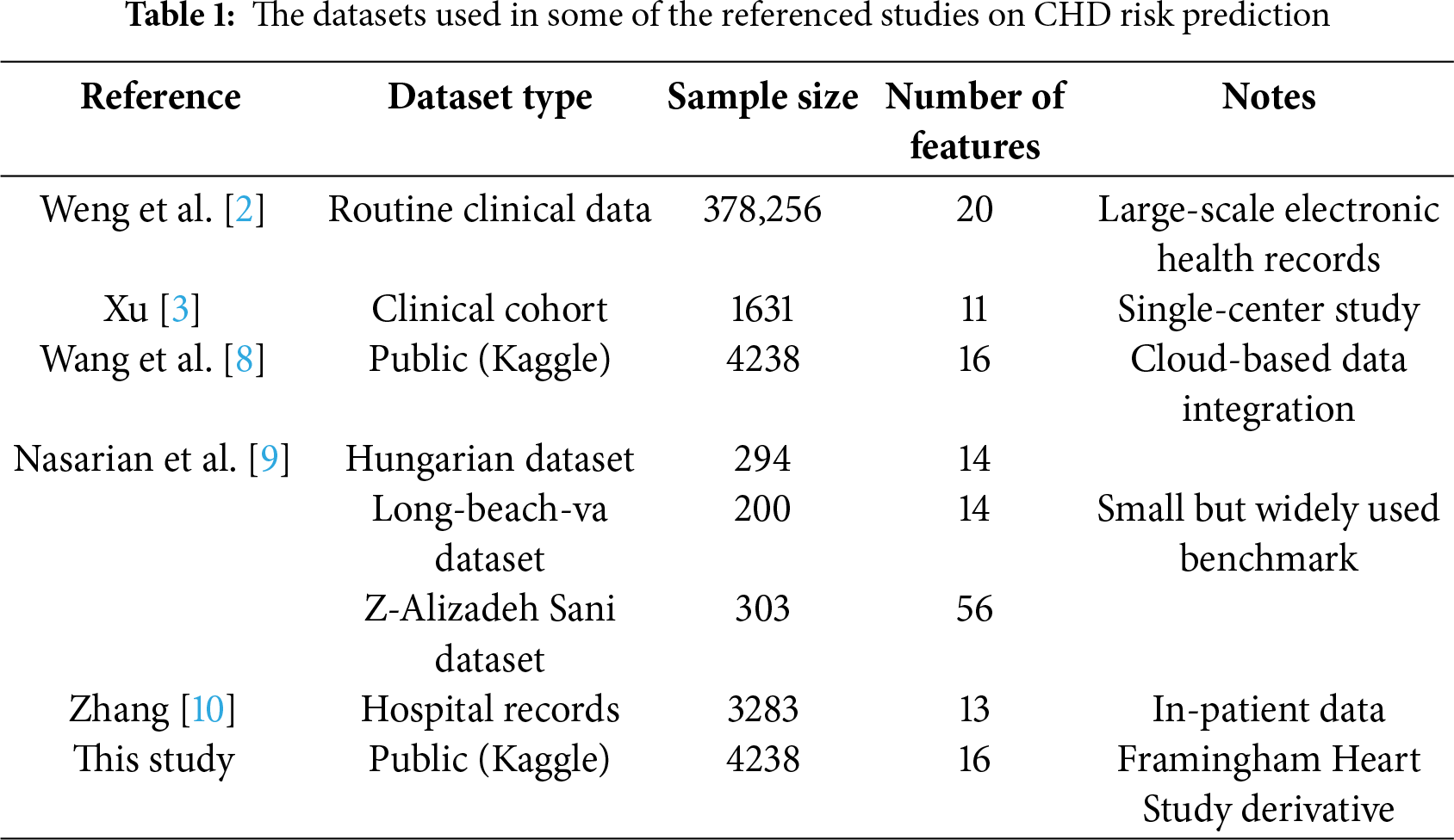
Table 1 summarizes the types and sizes of datasets used in some of the referenced studies on CHD risk prediction. This comparison helps to contextualize the dataset chosen for this study. The Kaggle CHD dataset used herein comprises 4238 samples with 16 features, which is comparable in size to many clinical and public health studies in this domain [2,3,9]. While some studies utilize larger administrative or multi-center cohorts [2,8,10], the selected dataset provides a substantial sample size for feature selection and model development. Its inclusion of both demographic and clinical variables aligns with common practices in the field, ensuring the representativeness and generalizability of our findings.

Based on the above studies on CHD risk prediction, it can be seen that the risk factors for CHD are complex and the selection of effective methods to screen for risk characteristics can make the risk prediction more efficient. Although some good progress has been made in existing research, several research gaps remain. First, many existing feature selection methods either focus solely on data-level characteristics (e.g., Filter methods) or algorithm-level performance (e.g., Wrapper/Embedded methods) [35], lacking an integrated approach that comprehensively considers both data intrinsic properties and model interpretability. Second, while some hybrid methods combine multiple techniques, they often fail to provide statistically interpretable feature importance scores that are both clinically meaningful and algorithmically robust. Third, there is a scarcity of studies that systematically integrate multi-angle feature importance measurements (e.g., combining mRMR, SHAP, and ARFS) with a robust feature subset selection strategy like SBS for CHD risk prediction. To address these gaps, this study proposes a novel framework that integrates multi-angle feature importance measurements with sequential backward selection to identify a minimal yet highly predictive set of CHD risk indicators. The following sections detail our data preparation, methodology, and experimental validation.

In addition, recent advancements in hybrid artificial intelligence (AI) models have significantly pushed the boundaries in cardiac disease detection and risk prediction. For instance, Attia et al. [36] developed an AI-enabled electrocardiogram (ECG) algorithm that can detect asymptomatic left ventricular dysfunction, a precursor to heart failure, with high accuracy, demonstrating the power of deep learning to extract hidden information from standard medical tests. Expanding on this, Raghunath et al. [37] showed that a deep learning model applied to ECGs could not only detect but also predict the future onset of atrial fibrillation, showcasing the predictive potential of AI in cardiology. Beyond single data sources, Poplin et al. [38] created a deep learning system that leverages retinal fundus photographs to predict cardiovascular risk factors, such as age, gender, and systolic blood pressure, illustrating the innovative and multi-modal nature of modern AI approaches in medicine. While these studies highlight the exceptional predictive performance of complex AI models, they often function as ‘black boxes’ and lack a rigorous, interpretable framework for identifying and ranking individual clinical risk factors. Our work addresses this gap by proposing a hybrid feature selection methodology that prioritizes both model performance and statistical interpretability, aiming to provide clinicians with a transparent and trustworthy tool for CHD risk assessment.

3  Data Preparation and Descriptive Statistical Analysis

To study CHD risk prediction, identify important risk assessment indicators, predict CHD risk more accurately and scientifically guide high-risk groups to effective prevention, this paper selects the CHD data set of Kaggle data website as the research sample. In this dataset, the feature “TenYearCHD” is the ten-year risk of CHD, with values of “0” and “1”, which is suitable for the binary prediction model. When the value of “TenYearCHD” is “0”, it means that the sample has no disease risk within 10 years. When the value is “1”, it means that the sample has disease risk within 10 years.

3.1 Data Preparation

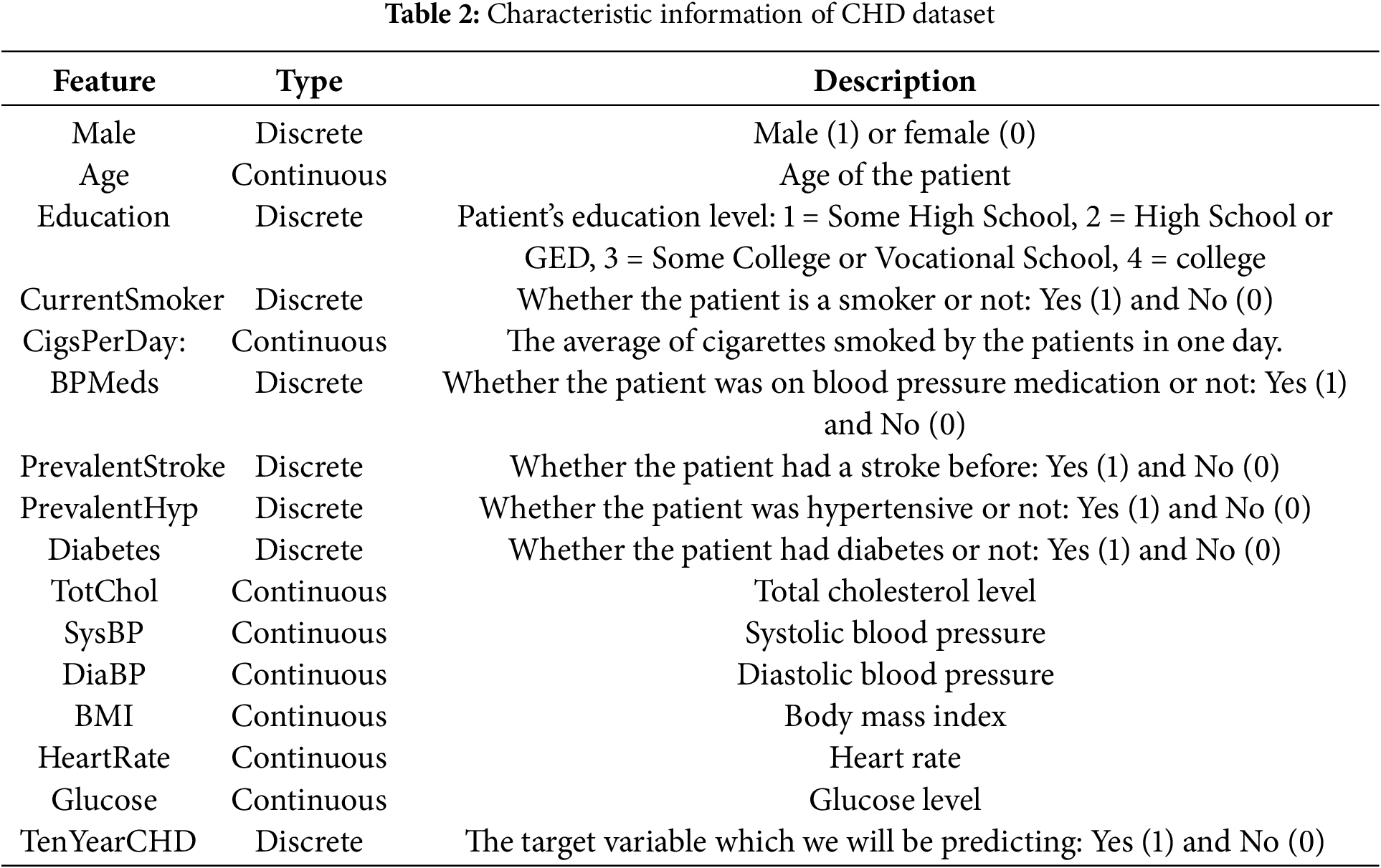
The dataset consists of 16 features and 4238 informative samples (The Framingham CHD dataset (https://www.kaggle.com/navink25/framingham, accessed on 01 September 2025)). Table 2 shows the type and description of each feature in the dataset. The first 15 features are basic information about the sample, this includes personal information (male, age, etc.), personal habits (currentSmoker, cigsPerDay, etc.), history of diseases (prevalentStroke, prevalentHyp, etc.), and various body indicators (totChol, BMI, heartRate, etc.). Among all features, there are 7 discrete features and 8 continuous features. Therefore, the basic characteristics of the dataset should be fully considered in the construction of the CHD risk prediction model, and the appropriate algorithm should be selected. In addition, some features have a small number of missing values, and appropriate methods should be chosen to fill in or remove the missing data during data preparation. Among all the sample information, 644 samples are diseased and 3594 are non-diseased at a ratio of 1:5.58, which means that this dataset is a non-equilibrium dataset with positive and negative samples.

(1) K-Nearest Neighbor (KNN) fills the missing value

Since the data set in this paper has a small number of samples and the number of diseased and non-diseased samples is non-equilibrium, removing samples containing missing values may reduce the number of diseased samples, so the K-Nearest Neighbor (KNN) algorithm [39] is chosen to fill in the missing data. KNN computes the distance between samples with missing data and other samples, and selects some samples with the smallest distance to compute the possible values of the missing data. For continuous data, the mean value of the column in which the missing values of K samples are located is chosen to fill in the missing data. For discrete data, which class has the largest number of samples among the K samples, the missing value samples will be classified into this class.

The specific features with missing values and the imputation techniques applied are as follows:

Continuous features (e.g., totChol, BMI, heartRate, glucose): Missing values were imputed using the mean value of the feature, as these variables typically follow a near-normal distribution in clinical populations and mean imputation helps preserve the overall distribution.

Discrete features (e.g., education, cigsPerDay, BPMeds): For ordinal discrete features like education, median imputation was used to maintain ordinality. For binary features like BPMeds, mode imputation was applied as it is most likely to reflect the prevalent category.

High missing rate features: Features with a missing rate exceeding 20% (e.g., BPMeds had ~15% missingness) were retained due to their clinical relevance in CHD risk assessment, as informed by cardiology literature.

Low variance features: Features with variance below a threshold of 0.01 (e.g., prevalentStroke due to its rarity) were retained despite low variability because of their established clinical significance in CHD pathogenesis.

The use of KNN imputation for the remaining features was motivated by its ability to leverage similarity between samples, which is particularly suitable for clinical datasets where patient profiles often cluster based on health indicators.

(2) SMOTE data equalization based on SMOTE

In the CHD dataset used in this paper, the ratio of positive and negative samples is 1:5.58, indicating that the dataset is non-equilibrium. To quantify the impact of class imbalance on model performance prior to feature selection and balancing, we established a baseline model using the original imbalanced dataset. A LightGBM classifier was trained using all 15 features with default parameters. The model achieved a high overall accuracy of 0.85 due to the majority class dominance. However, the precision for the minority class (CHD positive) was only 0.54, and the recall was 0.61, indicating poor detection of actual CHD cases. The F1-score for the positive class was 0.57, further highlighting the severe bias introduced by the imbalanced data distribution. These preliminary metrics underscore the necessity of both data balancing and robust feature selection to improve model sensitivity and clinical utility.

Due to the small amount of CHD data used in this paper, in order to preserve the data information, Synthetic Minority Oversampling Technique algorithm (SMOTE) [40] is used to oversampling the samples of the disease to get a balanced data set. SMOTE synthesizes new samples based on information from a small number of samples, thus achieving the goal of equalizing the number of positive and negative samples. In contrast to simple replicas of few class samples, SMOTE uses linear interpolation in generating new samples, greatly improving the quality of those generated, better preventing overfitting, and improving the classification performance of subsequent predictive models.

Given that m×n new samples need to be generated, the process of equating the CHD dataset with SMOTE is divided into the following steps.

Step 1: Calculate the Euclidean distance between each diseased sample and its similar sample, and record the first K samples closest to the diseased sample.

Step 2: Randomly select one of the K nearest neighbor samples to synthesize a new diseased sample. The synthesis method for the new sample is expressed as

xnew=xold+rand(0,1)×(xold−x′)(1)

where xnew represents the synthesized new sample, xold represents a minority sample in the original data set, rand(0,1) represents the random number between [0, 1], and x′ represents the selected nearest neighbor sample.

Step 3: Repeat step 2 several times and then generate a new sample based on the old one.

Step 4: Select m samples from all the minority samples and repeat steps 2–3 to obtain m×n new samples. This paper obtains a 1-to-1 balanced dataset between diseased and non-diseased samples, and after equilibrating the CHD dataset based on SMOTE, then construct a CHD risk assessment indicator system and a CHD risk prediction model.

3.2 Descriptive Statistical Analysis of CHD Data

The CHD dataset in this paper covers basic personal information of patients, disease history, various physical health indicators, and other different aspects of information. The dimensionality of the dataset is relatively high, so a basic descriptive statistical analysis of the data set is necessary before a relevant study can be carried out.

3.2.1 Data Distribution for Each Feature

Fig. 1 shows the data distribution for four discrete characteristics: male, education, prevalentHyp and prevalentStroke. It can be found that the sample size of females in the CHD dataset used in this paper is slightly larger than that of males. As the level of education increases, the number of samples decreases. In terms of history of disease, there were 2922 samples without hypertension, more than twice as many as those with hypertension, and only 25 of the 4463 data points included a stroke history. In this dataset, a small number of samples with a history of various diseases related to CHD need to be focused on.

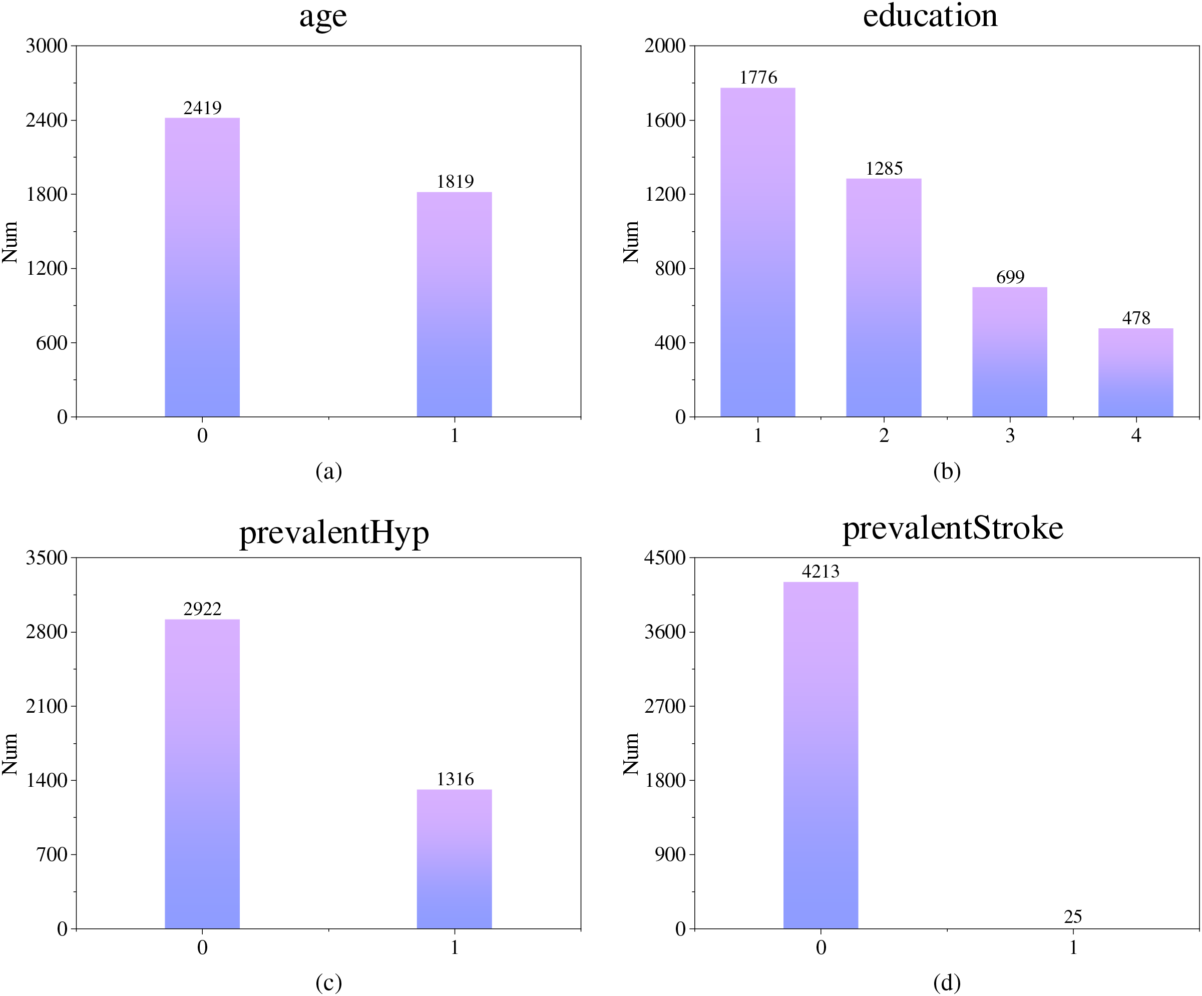
Figure 1: Distribution of partially discrete feature data (Subfigure (a) shows the gender distribution, subfigure (b) shows the distribution of educational level, subfigure (c) shows the distribution of hypertension cases, and subfigure (d) shows the distribution of stroke cases)

Fig. 2 shows the histograms of the data distribution and kernel density curves for four continuous features: age, BMI, sysBP and heartRate. As can be seen from Fig. 2a, most of the tested samples in this dataset are between 40 and 50 years old. In Fig. 2b, BMI represents the body mass index of the sample, and the normal value range is within the interval [18.5, 23.9]. Obesity is defined when the value is greater than or equal to 28. It can be seen that the BMI of the sample peaks around 26 and the number of obese individuals is close to half. The normal values of sysBP and heartRrate are within the interval [90, 140] and [60, 100], respectively. In Fig. 2c,d, these two features of most samples belong to the normal range, but nearly half of the samples still have symptoms of excessive systolic blood pressure or heart rate. It can be found that most of the samples in this dataset are middle-aged and elderly, and most of them have high BMI, sysBP or heartRate, so the above features may have a large impact on the risk of CHD.

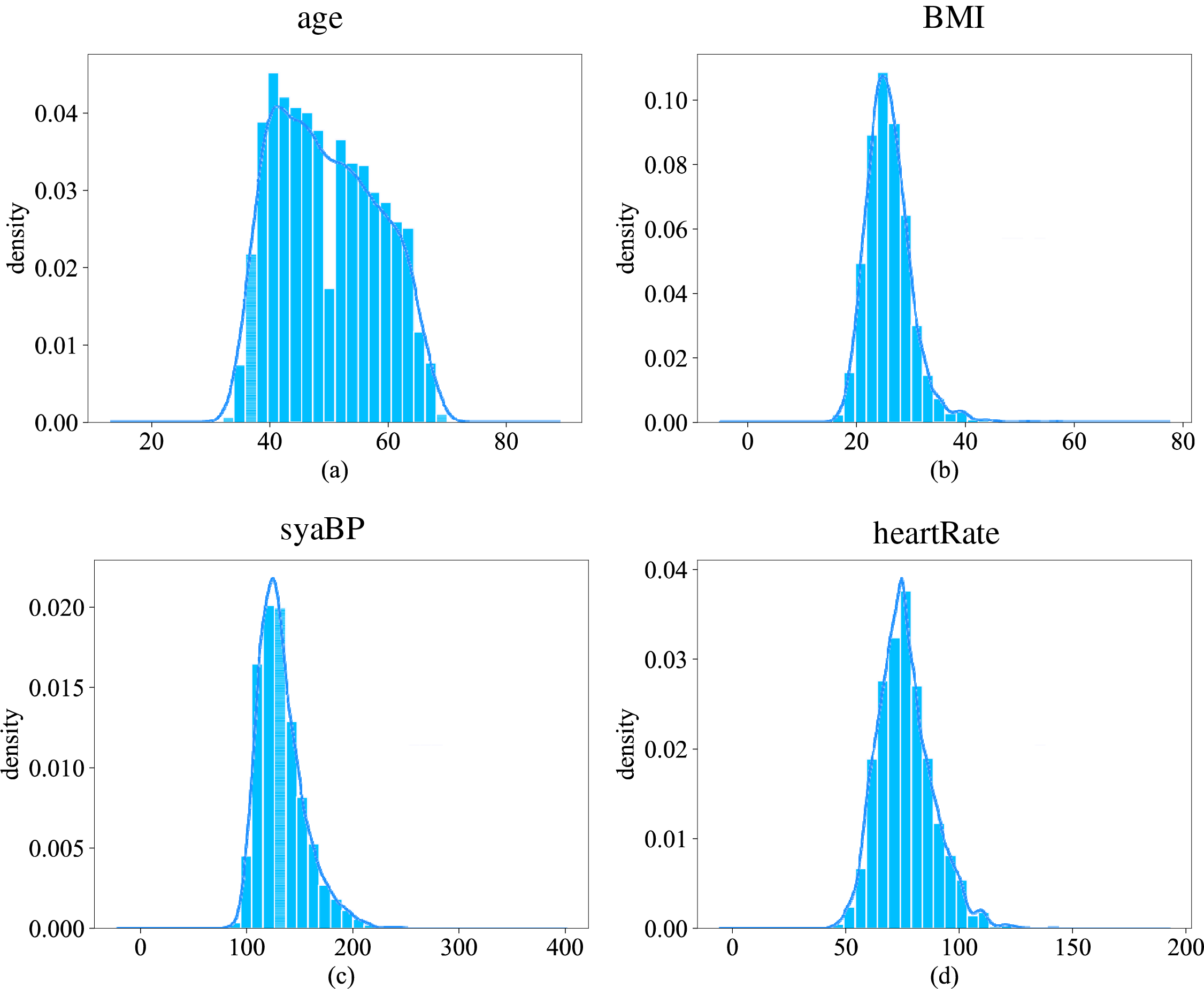
Figure 2: Distribution of partially continuous feature data (Subfigure (a) shows the distribution of ages, subfigure (b) shows the distribution of body mass index, subfigure (c) shows the distribution of systolic blood pressure, and subfigure (d) shows the distribution of heart rate)

3.2.2 Association of Each Feature with Disease Risk

Next, the relationship between features and the presence or absence of CHD was examined to characterize its impact on CHD risk.

First, the effect of individual features on CHD is investigated.

Fig. 3 shows the prevalence of disease in different age groups, with blue indicating non-disease and orange indicating disease. It can be seen that the number of people suffering from the disease increases with age. But starting at the age of 40, the total number of people in each age group has declined. It can be shown that with the increase of age, the rate of CHD increases rapidly, which reflects the aging of CHD. The risk of CHD in middle-aged and elderly groups may be higher than that in young groups.

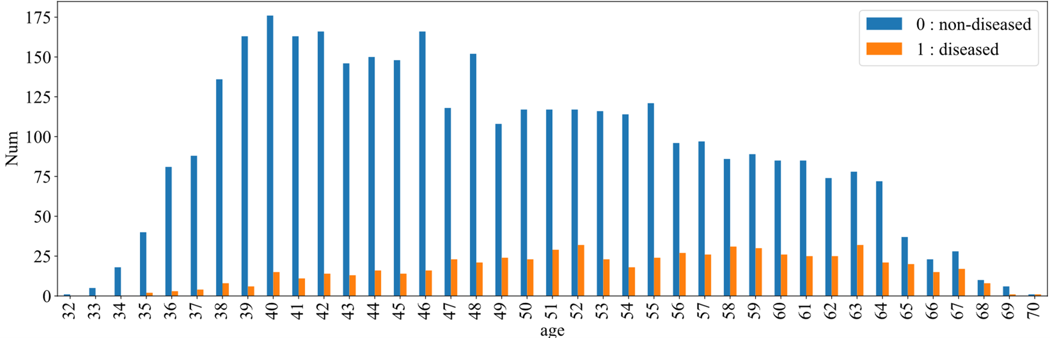
Figure 3: CHD among different age groups

Fig. 4 illustrates the effect of sample gender on CHD. The figure shows 0 for females and 1 for males, green for diseased and red for non-diseased. As can be seen from the figures, the number of non-diseased males is about two-thirds of the number of diseased females, even though the number of patients is essentially flat. In other words, the prevalence is significantly higher in the male sample than in the female sample. This can be explained by the fact that men are more likely to develop the disease than women.

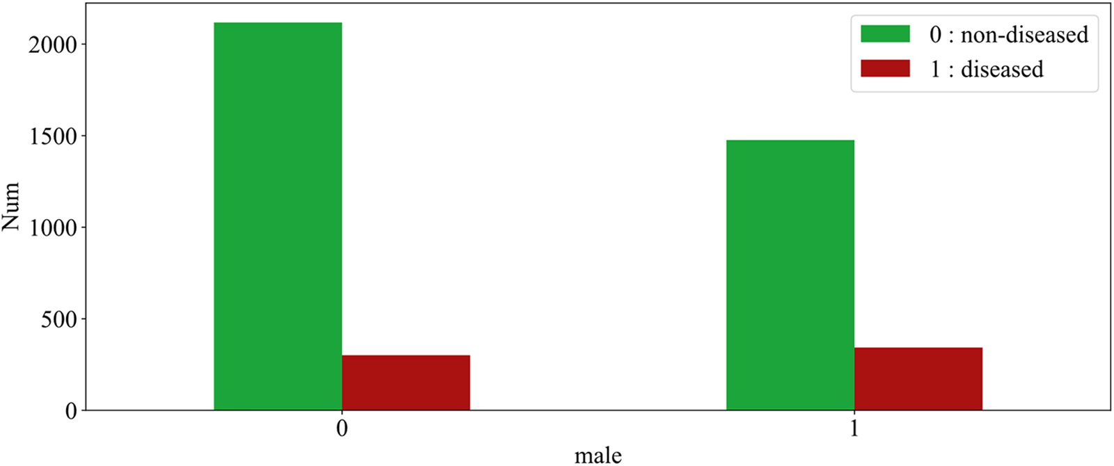
Figure 4: The effect of gender on CHD

Then, the effect of multiple variables on CHD is studied and the data is explored experimentally using the pdpbox library in Python.

Fig. 5 shows the effect of feature age and male on CHD, with disease presence on the horizontal axis and age on the vertical axis, male in blue and female in orange. For diseased samples, with the increase of age, the number of patients increased first and then decreased. Among them, male cases are mainly concentrated between 55 and 65 years old, and female cases are mostly concentrated between 50 and 60 years old. In addition, by observing the areas of the two colors, it is found that the areas of the two colors are basically the same in the samples with the disease, and the orange area is larger in the samples without the disease (there are more women), indicating that the female group has a lower risk of disease.

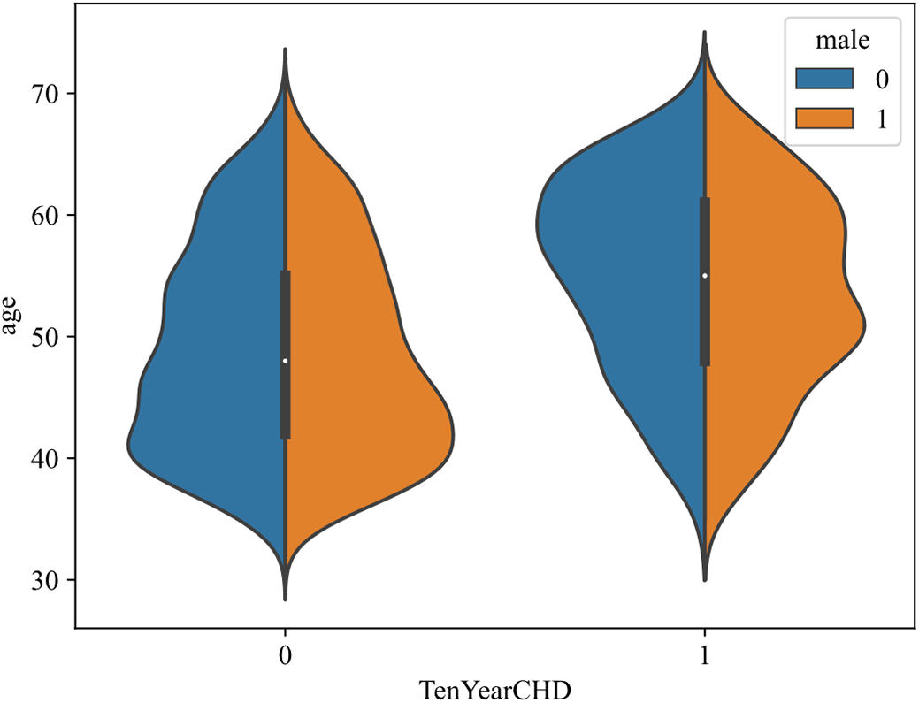
Figure 5: Effect of age and male on CHD

Fig. 6 shows the influence of different age and sysBP on CHD. The horizontal axis indicates age and the vertical axis sysBP. In the scatter plot, blue represents samples without disease and red represents samples with disease. By analyzing the scatter plot, the following conclusions can be drawn: with the increase of age, the number of patients with CHD also shows an increasing trend, and the number of patients with CHD is the largest within the range [65, 70]. With the increase of sysBP, the number of patients with CHD increased first and then decreased, and the number of patients with CHD was the largest within the range of [150, 200]. However, under the comprehensive consideration of age and systolic blood pressure, it can be seen that when the systolic blood pressure is between [100 and 150], there are also a large number of coronary heart disease samples in people over 60, which also suggests that older people have a higher probability of developing coronary heart disease.

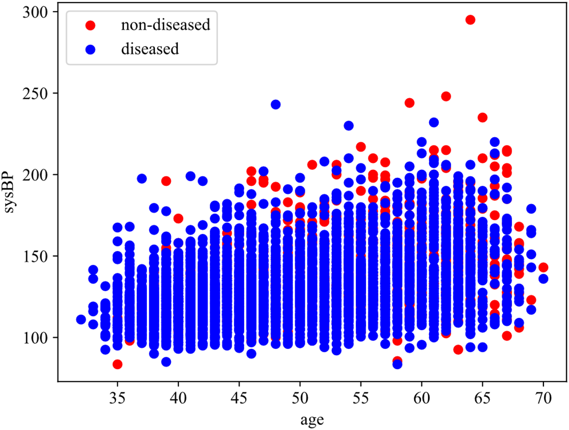
Figure 6: Effect of age and sysBP on CHD

4  CHD Risk Indicator Identification Method Based on Multi-Angle Integrated Measurements and SBS

Single feature selection method is somewhat flawed. This chapter proposes a feature selection method based on multi-angle integrated measurements and SBS, with the main ideas as follows: The mRMR algorithm and RF are chosen to identify CHD risk factors at the data and algorithm level, and RF is further integrated with SHAP theory and ARFS framework at the algorithm level to quantify the importance of each risk feature. Then, the importance score of each feature is obtained by combining the above three methods, and the optimal feature set is selected by the sequential backward selection method, which identifies the risk factors that have a greater impact on CHD. Finally, the risk assessment indicator system of CHD is established.

4.1 Multi-Angle Integrated Measurements

The rationale for integrating mRMR, SHAP-RF, and ARFS-RF stems from their complementary strengths in addressing different aspects of feature selection and their ability to collectively balance the bias-variance trade-off. mRMR provides a data-centric perspective by evaluating features based solely on their intrinsic statistical properties within the dataset. It identifies features with maximum relevance to the target while minimizing redundancy among themselves, thus reducing multicollinearity and model variance. However, it may introduce bias by ignoring the algorithm’s characteristics. SHAP-RF offers an algorithm-specific interpretation by quantifying the contribution of each feature to the predictions of a powerful ensemble model (Random Forest). It captures complex, non-linear relationships and interactions, providing insights into the model’s decision-making process. This reduces bias by accounting for the algorithm’s behavior but may increase variance due to model-specific dependencies. ARFS-RF contributes a statistical robustness perspective by assessing feature importance through algorithmic randomness testing. It provides statistically interpretable p-values that measure how significantly a feature disrupts the data’s randomness when permuted. This approach balances between data-driven and model-driven views, offering a rigorous framework for feature significance testing.

The integration of these three methods creates a more robust feature selection framework that mitigates the limitations of any single approach. While mRMR ensures foundational statistical soundness (reducing variance from redundant features), SHAP-RF incorporates model-specific performance insights (reducing bias from ignoring algorithm characteristics). ARFS-RF adds statistical rigor and interpretability, serving as a bridge between the data and algorithm perspectives. By combining their scores into a unified importance measure, we achieve a balanced evaluation that is neither overly dependent on the data structure nor overly specialized to a particular algorithm, thus optimizing the bias-variance trade-off in the final feature subset.

In the feature importance measurement stage, this paper changes the traditional computational approach and selects three methods from two levels of data and algorithm to measure feature importance scores from multiple perspectives and obtain significance scores for each feature, and screens the risk factors of CHD based on this. At the data level, mRMR is chosen to measure the importance of each risk factor in the original dataset, with the goal of minimizing the correlation between features and maximizing the correlation with categorical features. At the algorithm level, RF is chosen as the basic model, SHAP theory and ARFS framework are further integrated, and the importance of each feature is quantified from the two perspectives of the interpretation degree of each feature in the classification algorithm to the results and the statistical interpretability of the classification algorithm. Finally, the feature importance score obtained by the above three methods is treated as a 3D vector and its modulus length is calculated as the final feature importance score. The basic idea behind this section is shown in Fig. 7.

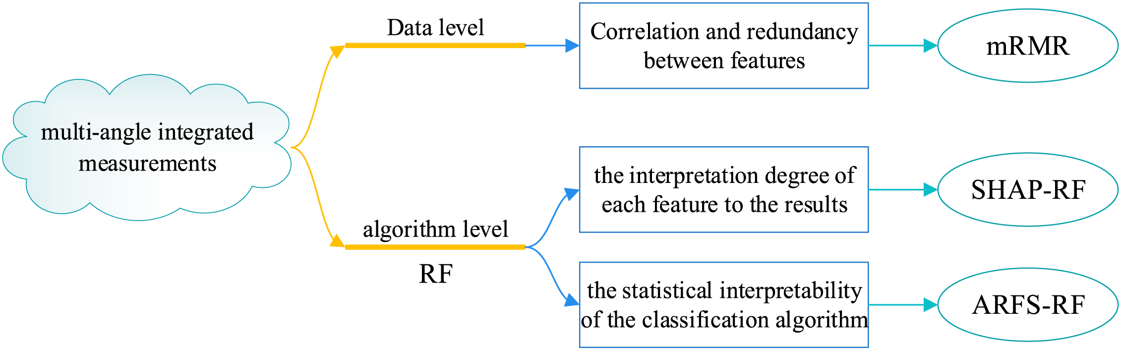
Figure 7: Basic idea of multi-angle integrated measurements

4.1.1 mRMR

At the data level, the Maximun Relerelevance Minimum Redundancy algorithm (mRMR) [41] is selected in this paper to calculate the feature important scores. The objective of mRMR is to minimize the correlation between features and maximize the correlation between features and target variables. It also considers the degree of correlation between features and features, features and target variables, and is able to fully mine the information in the data. The mRMR is a filter feature selection method based on Mutual Information (MI) between features [42], which does not require the participation of algorithms and has high computational efficiency, so it is widely used in practical applications [43].

In information theory, MI is a quantitative method used to calculate the interdependence between two variables [44]. It is further evolved on the basis of entropy, and the entropy of discrete random variable X is defined as

H(X)=−∑x∈Sp(x)log2⁡p(x)(2)

where S is the set of all possible values of X, and p(x) is the probability mass function of X (for discrete variables).

The joint entropy of two discrete random variables X and Y is defined as

H(X,Y)=−∑x∈S∑y∈Qp(x,y)log2⁡p(x,y)(3)

where p(x,y) denotes the joint probability density of the random variables X and Y, and Q is the set formed by all possible values of Y.

MI measures the interdependence between two random variables, which can also be said to be the part of information shared by two random variables, which is equivalent to the intersection of two sets. The relationship between MI and entropy is shown in Fig. 8.

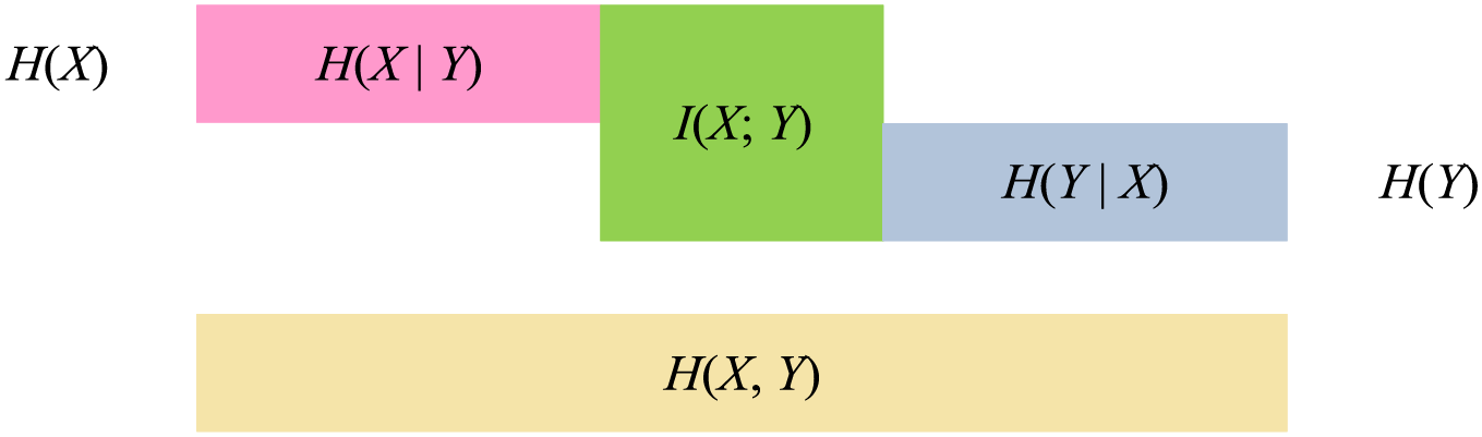
Figure 8: Diagram of the relationship between MI and entropy

The meaning of MI can be intuitively seen from Fig. 8, and its calculation method can be expressed as:

I(X;Y)=H(X)−H(X|Y)=H(Y)−H(Y|X)=H(X)+H(Y)−H(X,Y)=−∑x∈Sp(x)log2⁡p(x)−∑y∈Qp(y)log2⁡p(y)+∑x∈S∑y∈Qp(x,y)log2⁡p(x,y)=∑x∈S∑y∈Qlog2⁡p(x,y)p(x)p(y)(4)

Among the features of independent variable and dependent variable, when the MI value between the two features is large, it can be explained that they have a high degree of correlation, that is, the independent variable has a high degree of influence on the dependent variable.

The mRMR algorithm consists of the following two aspects:

(1) Maximum Relevance: extract the subset of features that are highly correlated with the category feature. That is to say, from all possible feature subsets of the original feature set M, a feature subset S with high correlation with the category feature is found.

The relevance of a feature subset S with the target class Y can be quantified as the average mutual information between each feature in the subset and the class:

D=1S∑t∈SI(Y;xt)(5)

where S represents the feature set, xt represents the column vector of the t-th feature, Y=[y(1),y(2),⋯,y(n)] represents the column vector of the target category feature in the data set, y(i) represents the category label (i=1,2,⋯,n) of the i-th instance in the data set, and I(Y;xt) represents mutual information.

Then, the maximum relevance can be expressed as:

maxt∈SD(S)(6)

(2) Minimum Redundancy: the maximum correlation between risk features and category feature can be supplemented by a minimum redundancy between features to minimize inter-feature dependencies. In practice, feature selection only depends on the maximum correlation between features and categorical feature, which can lead to large redundancy among features. That is to say, features that are highly correlated with the target variable may also be highly correlated with each other, which leads to more redundant features in the selected feature subset. On the basis of maximum correlation, appropriate deletion of some redundant features has little impact on classification result.

Similarly, the redundancy among the features within the subset S can be quantified as

R=1S′2⁢∑k,t∈SI⁡(xk;xt).(7)

Then, the minimum redundancy can be expressed as:

mint∈SR(S).(8)

The mRMR algorithm is a combination of maximum relevance degree and minimum redundancy degree. The purpose of mRMR algorithm is to extract an effective feature subset from the original feature set. The feature subset should contain as much information as possible from the original feature set, and it should be concise enough to reduce the computational complexity. The idea of mRMR can be simplified as follows: the selected feature subset has the maximum correlation with the category feature, while each feature in the selected feature subset has a low correlation. Therefore, the implementation of mRMR algorithm can be realized in the following two ways:

Mutual information difference (MID):

Φ1=D−R,(9)

maxΦ1(D,R).(10)

Mutual information quotient (MIQ):

Φ2=D/R,(11)

maxΦ2(D,R).(12)

In this paper, MID is used to implement mRMR algorithm, and incremental search method is used to select effective features that meet the requirements. Assuming that the selected feature set is Sk−1, the following conditions should be met when the k-th feature is screened from the alternative feature set each time:

maxk∈M−Sm−1[I(Y;xk)−1|Sm−1|t∈Sm−1∑t∈Sm−1I(xk;xt)],(13)

Eq. (13) defines the core criterion for selecting the k-th feature in the incremental search process of the mRMR algorithm. The objective of this equation is to identify the feature that maximizes the mutual information with the target variable Y (relevance) while minimizing the average mutual information with all features already selected in the set Sm−1 (redundancy). The variables in the equation are defined as follows:

M: The complete set of all original features.

Sm−1: The subset of m−1 features that have already been selected in previous steps.

xk: The candidate feature under consideration from the set of remaining features M−Sm−1.

xt: A feature already residing in the selected subset Sm−1.

I(Y; xk): The mutual information between the target variable Y and the candidate feature xk, measuring their relevance.

I(xk; xt): The mutual information between the candidate feature xk and an already-selected feature xt, measuring their redundancy.

|Sm−1|: The cardinality (number of features) of the currently selected subset Sm−1.

Based on the importance scores of features computed by the mRMR algorithm, it can effectively balance relevance and redundancy, effectively removing redundant features while ensuring maximum relevance. However, since only the data itself is considered in the computation and no classification algorithm model is introduced, the impact on the classification effect cannot be guaranteed. Therefore, the RF algorithm will be introduced in the following study to evaluate the risk factors for CHD, and the role of features in the classification model will be investigated from an algorithmic point of view. A more accurate and effective feature subset is selected through comprehensive research from the data and algorithm level.

The mRMR algorithm was implemented using the mrmr Python package. The mutual information was estimated using the mutual_info_classif function from the scikit-learn library with default parameters. The number of features to select was set to 15 (all features) to obtain a complete ranking. The MID criterion was used as the optimization objective, as defined in Eq. (11). The discrete features were preprocessed using label encoding, while continuous features were used directly.

4.1.2 SHAP-RF

As an ensemble learning algorithm, RF [45] integrates a variety of weak classifiers to obtain a strong classifier. It has the advantage of effectively reducing the risk of erroneous classification, as well as improving the generalization ability of the model and reducing overfitting. Moreover, RF is a ML method based on feature partitioning, which can flexibly adapt to datasets containing classification features and numerical features [46]. The CHD dataset used in this paper has both classification features and numerical features. Some classification features have a strong influence on CHD, and the prediction results of CHD risk can only be yes or no. Due to the discretization of features in the CHD dataset, RF has some advantages for feature selection.

The RF algorithm builds a model based on Bagging with some samples randomly selected from the original training set. The construction process of the model has strong randomness [47]. The whole construction of the RF model consists of three stages: the first stage is to sample the dataset to obtain the training set of each decision tree, the second stage is to generate each decision tree, and the third stage is to generate the RF model. In the modeling process of RF, random displacement of each random variable is carried out and new out-of-bag data is generated for testing. The variation values of prediction error rate before and after random displacement is scored, and the feature importance score of each variable is further obtained.

In the RF model, the feature importance score calculated by the traditional random permutation method can only reflect the general importance degree of the feature in the classification model, but cannot explain the influence degree of each feature in the model on the final prediction result. SHAP value can explain various classification and regression models, and is used to quantify the contribution of each feature to model prediction results [31]. In the process of predicting each sample with the classification model, the SHAP value is the contribution of each feature to the predicted value of the sample. The basic idea is as follows: First, the marginal contribution of each feature is computed. Second, the marginal contribution of each feature in all feature sequences is computed separately. Finally, all marginal contributions of each feature are averaged to obtain the SHAP value of that feature. The feature importance score obtained by SHAP takes into account the influence of single variable and feature group on CHD, as well as the possible synergistic effect between features, which can explain whether each feature contributes positively or negatively to the sample prediction result, which is a very comprehensive feature importance calculation method [48].

The interpretation principle of SHAP on a certain sample can be represented as Fig. 9. In Fig. 9, yellow indicates a positive feature contribution to the sample prediction result, while blue indicates a negative feature contribution to the sample prediction result.

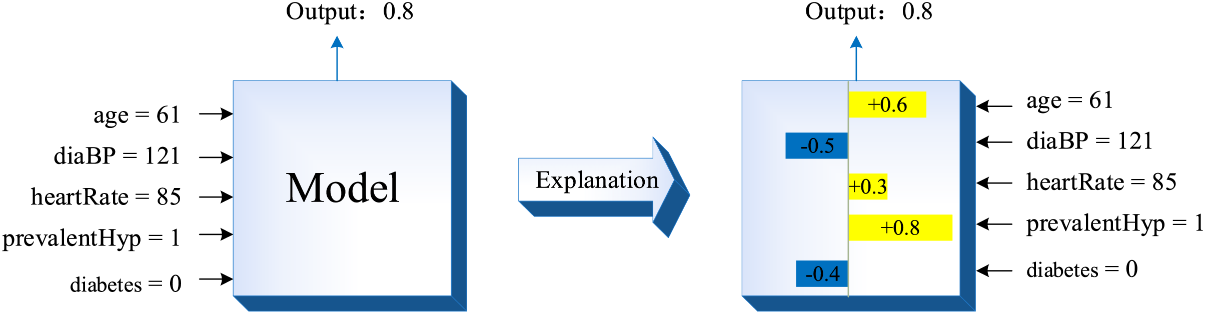
Figure 9: The interpretation principle of SHAP

Different samples may have different SHAP values for the same feature, and the final output value of the samples in the decision tree can be expressed as the sum of the SHAP values of each feature, which satisfies the additivity of the contribution values of the features. Assuming that f(x) denotes the predicted value of the sample in the decision tree, the following equation can be satisfied:

f(x)=g(z′)=ϕ0+∑i=1Mϕizi′,(14)

where ϕ0 is the base value (the expected value of the model output), ϕi is the SHAP value attributing the contribution of the i-th feature to the prediction for that specific sample, and zi′∈{0,1}M represents how many features are included in the decision path where the sample is located among all M features. For a certain sample, if feature i is not in its decision path, then the SHAP value of the sample for feature i is equal to 0 (ϕi=0), that is, feature i does not contribute anything to the final predicted value of the sample.

For a given sample, the contribution of the i-th feature in the dataset to its predicted value, the SHAP value (ϕi) is calculated as follows.

ϕi=∑S⊆N{i}|S|!(M−|S|−1)!M![fx(S∪{i})−fx(S)].(15)

Eq. (15) provides the exact calculation for the SHAP value ϕi or a given feature I and a single sample. The objective of this equation is to fairly distribute the contribution of each feature to the difference between the model’s prediction for this sample and the average prediction (base value), considering all possible subsets of features. The variables are defined as:

ϕi: The SHAP value to be computed for the i-th feature, representing its additive contribution to the prediction.

N: The complete set of all M features.

S: A subset of features that does not include the i-th feature (S⊆N∖{i}).

|S|: The size (number of features) of subset S.

M: The total number of features.

fx(S∪{i}): The prediction of the model for the sample when it only uses the features in the subset S plus the feature i.

fx(S): The prediction of the model for the sample when it only uses the features in the subset S.

The difference [fx(S∪{i}) − fx(S)] is the marginal contribution of feature I when added to subset S.

The above equation shows that, for a sample, the SHAP value of the i-th feature is the average value after marginal contributions from each feature are obtained and summed. Since a variety of feature combinations can be extracted to form a subset S under all features, the SHAP value of feature i is a comprehensive score under the enumeration of all possible feature subsets, considering the influence of other features on feature i besides itself.

Assuming that there are m samples and n features in the dataset, the SHAP values of each sample under each feature can form a m×n dimensional matrix, and then the importance score of each feature can be defined as the mean absolute value of the columns of the matrix.

4.1.3 ARFS-RF

ARFS-RF is a feature selection method based on algorithm randomness and RF. It combines ML methods and statistical testing methods to propose a statistically interpretable p-value to calculate the feature importance score. Among them, ARFS is a feature selection framework based on algorithm randomness [34]. It uses the ML algorithm to calculate the inconsistency score of each instance belonging to the data distribution, then carries out the algorithm randomness test to obtain the p-value, and finally defined the importance score of each feature as the decrease of the p-value before and after the random arrangement of the feature [34].

(1) ARFS framework

The Kolmogorov algorithm randomness theory defines a randomness detection function when describing the randomness of sample sequences [49]. Suppose z={z1,z2,⋯,zn} is a set of independently equally distributed sample sequences, Z represents the sample space, and zi∈Z(i=1,2,⋯,n) all come from some random model with probability distribution P. For a sample sequence of length n, define the randomness detection function as t:Zn→[0,1], then t satisfies:

(1) For all n∈N, λ∈[0,1] and P:

Pn{z∈Zn:t(z)≤λ}≤λ.(16)

(2) The randection function is computable since the upper half.

A randomness detection function with a value t(z) called the p-value represents the level of randomness of the data series. A larger p-value indicates that the sample sequence z is generated by a random model to some extent. That is, the algorithmic randomness tests for data series is very similar to the independent identical distribution test, and the independent identical distribution hypothesis can also be referred to as the algorithmic randomness hypothesis in statistics.

According to algorithmic randomness theory: when a data sequence undergoes a large change, the level of randomness of the data sequence decreases significantly, that is, the p-value decreases significantly. That is, when all values of a feature are randomly permuted, the more the p-value decreases, the more important the feature is in the data distribution. Therefore, the feature importance score is defined as the value by which the p-value decreases after random permutation of that feature.

P(Xj)=p0−pj,(17)

where P(Xj) denotes the importance score of feature Xj, p0 denotes the p-value of the original sequence, and pj denotes the p-value after randomly displacing feature Xj.

(2) The calculation of p-value

The Conformal Predictor (CP) extends the Kolmogorov algorithm stochasticity test as a machine learning framework [50]. Suppose the sample sequence zn−1=(z1,z2,⋯,zn−1) is known, each instance is zi=(xi,yi), xi∈X is the feature vector of sample zi, yi∈Y={0,1} is the label of the category to which sample zi belongs, and xn is the data sample to be tested. Form a test sample zny=(xn,y) of xn with each possible category, and then form a sequence of test sample zny and training sample zn−1:

zn,y={(z1,z2,⋯,zn−1,zny),y∈Y={0,1}}.(18)

Define the sample singularity detection function α:

Λ:zn,y→αn,y,y∈Y={0,1}.(19)

All samples in zn,y are mapped separately for singular values to obtain a set of sequences of singular values αn,y={α1,α2,⋯,αn−1,αny}. Then the p-value of the algorithmic randomness level for zn,y can be calculated by the following equation:

p=|{i=1,2,⋯,n−1;αi≥αny}|+1n.(20)

(3) The design of sample singularity detection function

RF can generate a proximity matrix for all examples xi [45]. After a tree is grown, all training data is put into the tree, and if instances xi and xj are in the same terminal node, their proximity values are increased by one. Finally, the number of trees is divided to normalize the proximity in order to obtain their proximity metric proxij.

If there are N trees in the random forest and the initial proximity of instances xi and xj is 0, the proximity of two instances in each tree may increase or decrease by 1, and the final calculated proximity is n(n≤N). Then, the proximity measure of instances xi and xj is proxij=n/N.

The sample singularity detection function is defined as:

αi=∑j=1Kproxij−yi∑j=1Kproxijyi,i=1,2,⋯,n,(21)

where proxij−yi denotes the j-th largest proximity between an instance xi and an instance different from yi, proxijyi denotes the j-th largest proximity between an instance xi and an instance with yi.

From the above formulation to define the sample singularity detection function, we can see that if the proximity between two instances xi and xj with the same label is larger, while the proximity between two instances xi and xj with different labels is smaller, the corresponding sample singularity detection function takes a smaller value. Therefore, the sample singularity detection function defined using the RF model proximity metric can more accurately reflect the inconsistency of the instances with respect to the data distribution.

In summary, the steps for computing feature importance scores based on ARFS-RF can be described as follows.

Step 1: A RF model is constructed using the original dataset D and the proximity matrix is derived.

Step 2: The initial algorithmic randomness level p0 of the dataset is calculated according to Eqs. (19) and (20).

Step 3: Randomly permuting the values of the first feature yields a new set of dataset D1.

Step 4: The RF model is constructed according to Step 1 and Step 2, and the randomness level of the algorithm is calculated under the new dataset.

Step 5: Calculate the importance scores of the features according to Eq. (17).

Step 6: Repeat Step 3 to Step 5 to compute importance scores for each feature and rank them in descending order.

4.1.4 Calculation of Feature Importance Scores

After calculating the feature importance scores of all three methods, since different methods have different scales, it is necessary to unify the scales when calculating the composite scores of the features, and the feature importance scores obtained by each method are normalized to values between [0, 1] by polar differences. The calculation formula is as follows:

xi′=xi−minxmaxx−minx,(22)

yi′=yi−minymaxy−miny,(23)

zi′=zi−minzmaxz−minz,(24)

where xi, yi and zi are the original feature importance scores computed by mRMR, SHAP-RF and ARFS-RF, respectively. xi′, yi′, and zi′ are the values after normalization by the three methods, respectively. Take mRMR algorithm as an example, maxx and minx are the maximum and minimum feature importance scores under the mRMR algorithm, respectively.

The normalized importance score of each feature is mapped to a 3D vector ci→=(xi′,yi′,zi′). The modal length of the vector ci→ is the final obtained feature importance score, expressed as

|ci→|=xi′2+yi′2+zi′2.(25)

The flowchart of the multi-angle integrated measurements is shown in Fig. 10.

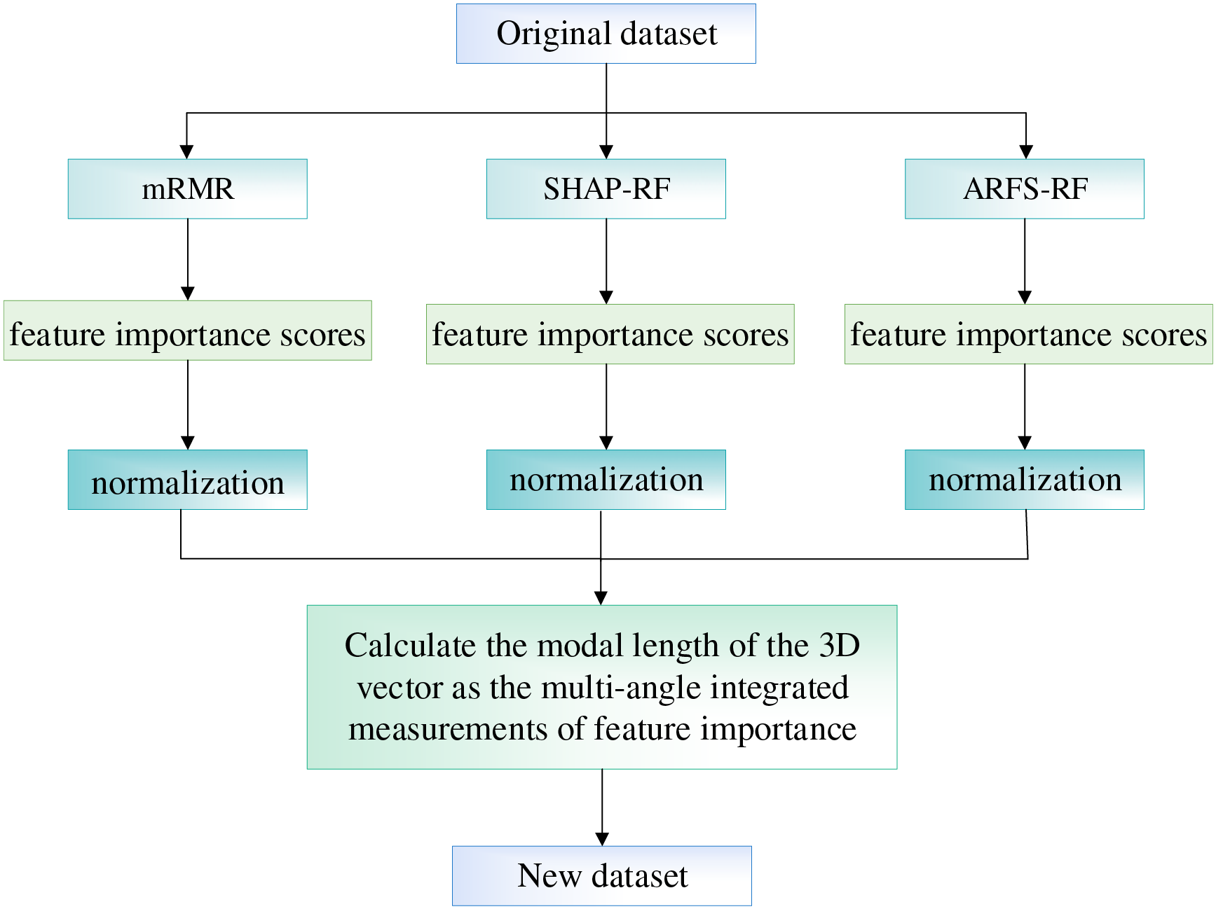
Figure 10: The flowchart of the multi-angle integrated measurements

4.2 Risk Indicator Screening Based on SBS

For the basic features of the patient sample in the CHD dataset, the data and algorithm levels are analyzed in an integrated manner to measure the importance of the features. In order to obtain the best feature subset, the feature subset is screened based on the integrated feature ranking obtained from the multi-angle integrated measurements to reduce the number of feature dimensions and improve the computational efficiency of the subsequent classification prediction model. In this paper, we aim to maximize the classification accuracy of the LightGBM model and use Sequential Backward Selection (SBS) to screen the data set for CHD risk evaluation indicators after the comprehensive ranking of features. First, all ranked features are fed into the LightGBM model for training, and the accuracy of the model is output. Second, a new dataset is obtained by removing the least important features one at a time. Then, the new dataset is input into the LightGBM model and output the accuracy of the model. Finally, the trend of model accuracy as the number of features in the dataset decreases is plotted and the subset of features with the highest accuracy is selected as the result of the choice of CHD risk metric.

The specific algorithm flow is shown in Fig. 11.

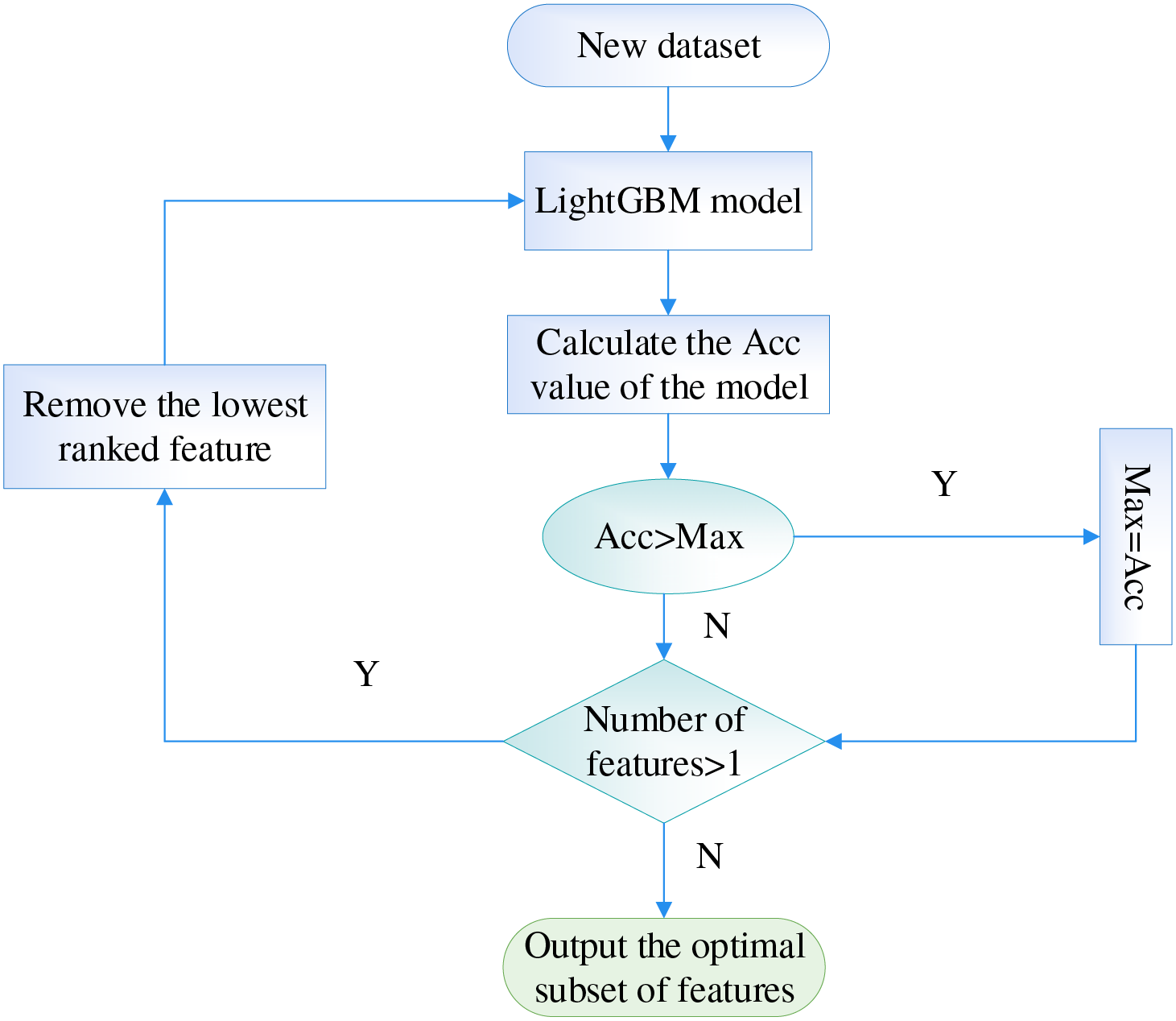
Figure 11: The flowchart of screening risk indicators at SBS stage

4.3 CHD Risk Indicator Identification Method Based on Multi-Angle Integrated Measurements and SBS

For the 15 basic patient information features in the CHD dataset, this paper proposes a feature selection method based on multi-angle integrated measurements and SBS for the construction of a CHD risk evaluation index system. First, in the multi-angle integrated measurements stage, mRMR, SHAP-RF and ARFS-RF are selected from the data and algorithm levels to calculate the importance of the features. Then, the three types of feature importance scores are normalized to eliminate the influence of the magnitude, and the modal length of the 3D vector is used as the final feature importance metric. Finally, the LightGBM model is selected as the classifier, and the risk indicators with the lowest feature importance scores were sequentially removed using SBS, so as to select the subset of features with the highest model accuracy as the input data for the construction of the coronary heart disease risk prediction model.

In fact, the LightGBM (Light Gradient Boosting Machine) model was selected as the classifier for the SBS process due to its several key advantages that are particularly suited for this study: (i) High Efficiency and Speed: LightGBM uses a novel technique called Gradient-based One-Side Sampling (GOSS) and Exclusive Feature Bundling (EFB) to handle large-scale data efficiently, which significantly reduces computational time during the iterative process of SBS. (ii) Low Memory Usage: Its histogram-based algorithm requires less memory compared to other gradient boosting frameworks, making it ideal for rapid multiple iterations. (iii) Superior Accuracy: LightGBM grows trees leaf-wise (best-first) rather than level-wise, which often leads to lower loss and higher accuracy, providing a reliable metric for evaluating feature subsets. (iv) Strong Handling of Imbalanced Data: Although our dataset was balanced using SMOTE, LightGBM inherently performs well on imbalanced datasets, which is a common scenario in medical diagnostic problems. (v) Support for Categorical Features: It provides excellent native support for categorical features, which aligns well with the mixed data types (continuous and discrete) in our CHD dataset. Given that the SBS process requires building a model for each feature subset candidate, the combination of high speed and high accuracy makes LightGBM an optimal choice for the evaluation metric in our wrapper-based feature selection method.

To provide a detailed description of the integrated model components, we outline the complete forward pass of the proposed methodology as follows:

(1) Input data preparation. The input consists of the preprocessed CHD dataset with 15 features after KNN imputation and SMOTE balancing. Each sample is represented as a feature vector x ∈ R15.

(2) Multi-angle feature importance scoring.

mRMR Module: Computes feature importance scores based on mutual information between features and the target, and between features themselves. Output: a vector smRMR ∈ R15.

SHAP-RF Module: A Random Forest classifier is trained on the dataset. SHAP values are computed for each feature across all samples, averaged to produce an importance vector sSHAP ∈ R15.

ARFS-RF Module: Algorithmic Randomness Feature Selection is applied using RF to compute p-value decreases for each feature, yielding sARFS ∈ R15.

(3) Score normalization and fusion.

Each score vector is min-max normalized to [0, 1]. The three normalized vectors are treated as a 3D vector per feature. The final importance score for each feature is the Euclidean norm of the vector expressed by Eq. (25).

(4) Feature Ranking and SBS Selection. Features are ranked in descending order of the modal length of the vector ci→ expressed by Eq. (25). The SBS process begins with the full set of 15 features. In each iteration, the lowest-ranked feature is removed, and a LightGBM model is trained on the remaining features. The accuracy is recorded. This continues until only one feature remains.

(5) Output: The feature subset with the highest LightGBM accuracy is selected as the final set of risk indicators. The output is a reduced feature vector, where k = 11 in our case.

This forward pass ensures that the feature selection process is both interpretable and reproducible, integrating data-level and algorithm-level perspectives through a structured pipeline.

The flowchart of the feature selection method based on multi-angle integrated measurements and SBS is shown in Fig. 12.

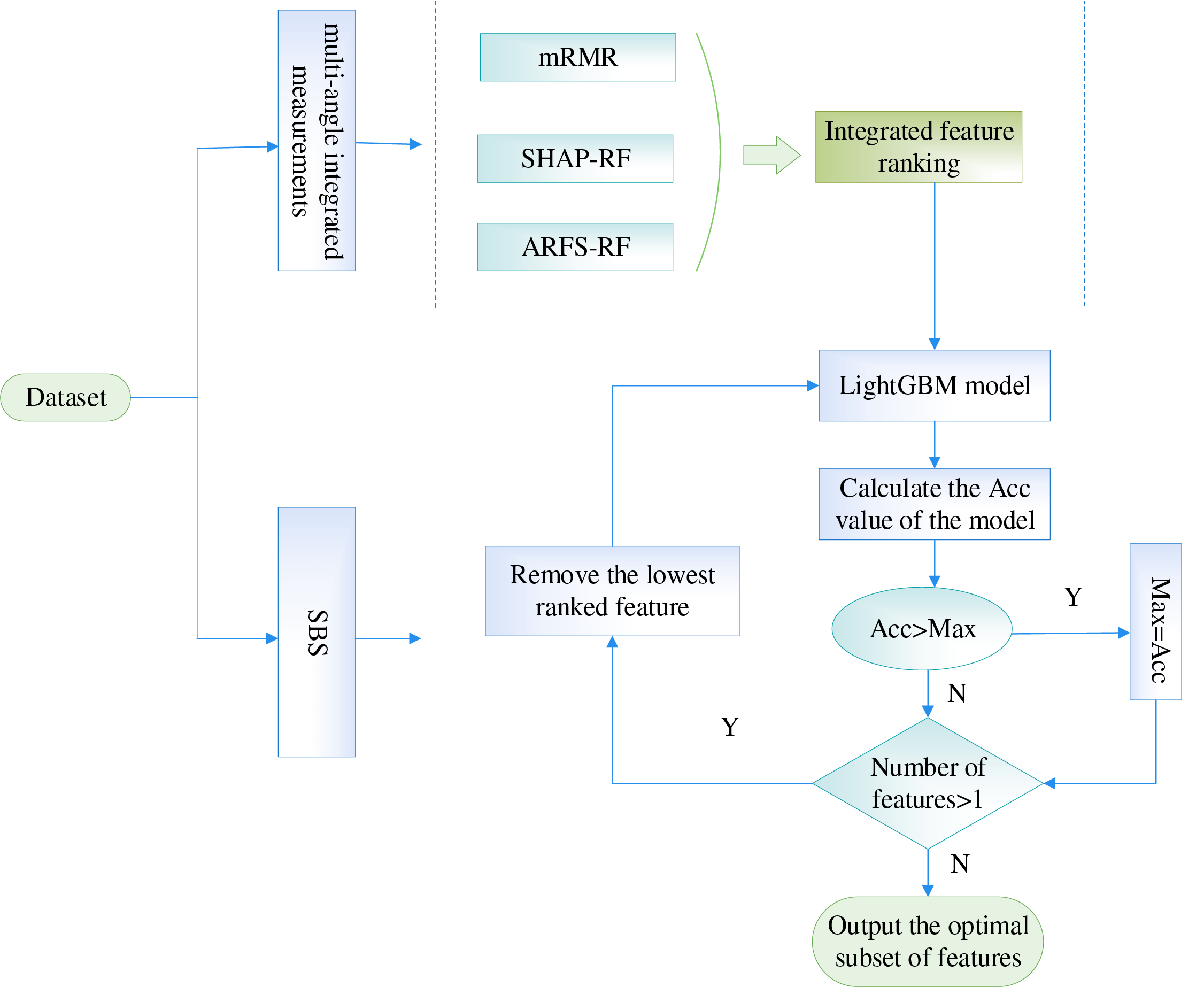
Figure 12: The flowchart of the feature selection method based on multi-angle integrated measurements and SBS

4.4 Risk Indicator Identification Based on CHD Dataset

4.4.1 Calculation of the Importance of CHD Risk Features Based on Multi-Angle Integrated Measurements

For the basic features of the patient samples in the CHD dataset, we analyze them integrally at both the data and algorithm level to quantify the degree of importance of the features. The mRMR algorithm is chosen at the data level to compute importance scores for each risk feature in the dataset in terms of relevance and redundancy. The RF algorithm is chosen as the classification model at the algorithm level, taking into account both the explanatory power of each feature on the classification results and the statistical interpretability of the classification algorithm. First, the importance scores of each feature are computed based on the three methods of mRMR (Maximum Relevance Minimum Redundancy), SHAP-RF (SHapley Additive exPlanations-Random Forest), ARFS-RF (Algorithmic Randomness Feature Selection Random Forest), respectively. Then, the feature importance scores obtained by the three methods are normalized and the modal length of the 3D vector is calculated as the final feature importance score.

The multi-angle feature importance scoring does not involve a weighted multi-objective function in the traditional optimization sense. Instead, each method (mRMR, SHAP-RF, ARFS-RF) computes a score independently. These scores are normalized and combined via Euclidean norm (as described in Section 4.1.4), which implicitly treats each angle equally. No manual weighting is applied.

In the mRMR algorithm, MID is selected to measure the correlation and redundancy between features in this paper. In the RF algorithm, the proportion of training set samples is set to 70% to construct the classification model. Table 3 shows the feature importance scores obtained by the three methods of mRMR, SHAP-RF and ARFS-RF.

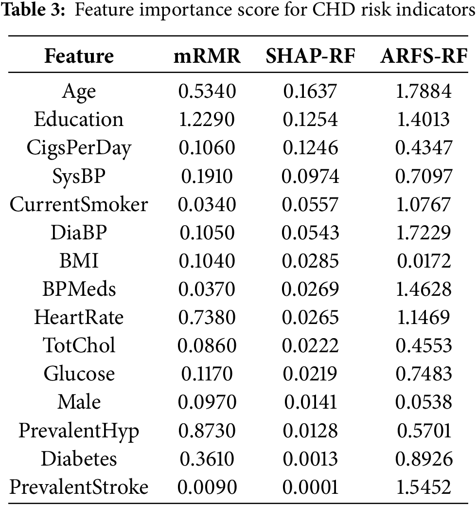
According to the feature importance scores of CHD risk factors in Table 3, it can be seen that the feature importance scores of “age” and “education” are higher in all three methods, which indicates that these two factors play a very important role in the likelihood of CHD. Among the importance scores of each risk factor obtained by the mRMR algorithm, the values of “cigsPerDay” and “currentSomker” are 0.106 and 0.009, respectively, indicate that these two factors have a certain influence on whether to have the disease or not and have a large correlation, so the feature importance score of “currentSomker” is low in the mRMR algorithm.

The combined feature importance scores are further computed and the results obtained are shown in Table 4. Fig. 13 shows a histogram of the importance scores for each feature.

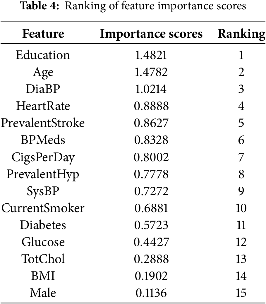
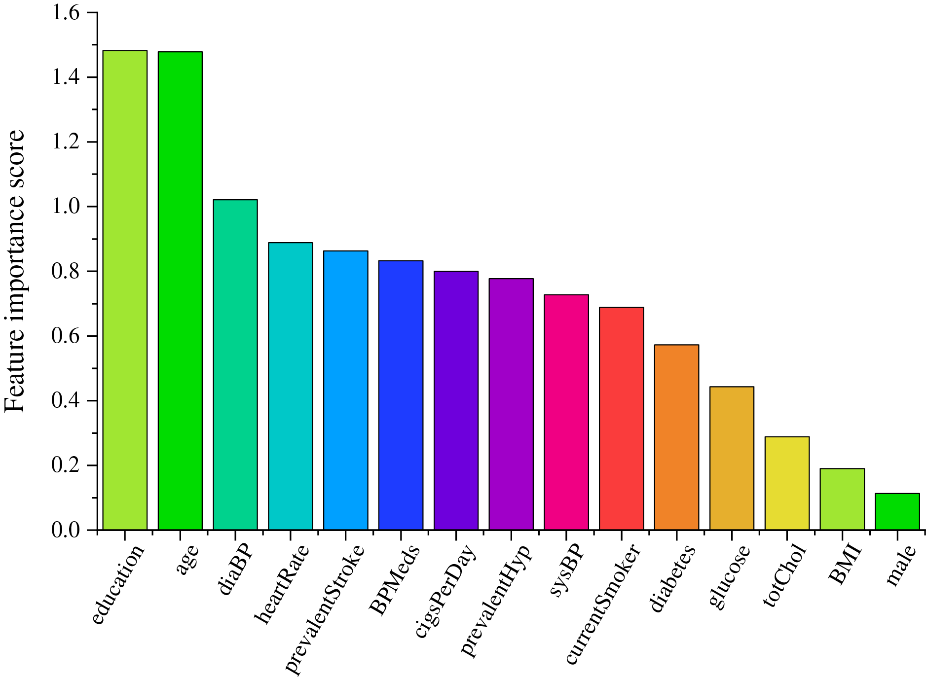
Figure 13: Feature importance score histogram

4.4.2 Selection of Risk Indicators for CHD Based on SBS

In this paper, the features with the lowest feature importance scores are sequentially removed by SBS on the basis of the feature importance measures. Starting from a complete dataset containing 15 features, the features with the least degree of importance are eliminated each time, and the LightGBM classification model is constructed, then take the classification accuracy as the assessment indicator. The features are compared with the assessment indicator of the previous round after each elimination, and the larger value is recorded as Max. Until the subset of features with the highest accuracy is selected, and the CHD risk assessment indicator system is constructed based on this.

The LightGBM classifier was implemented using the lightgbm Python package. To ensure optimal performance and avoid overfitting, we employed a comprehensive optimization strategy. Concretely, we conducted Bayesian optimization with 5-fold cross-validation using the Optuna framework over 100 trials to identify the optimal hyperparameters. The search space included:

num_leaves: [15, 255]

learning_rate: [0.01, 0.3] (log-scale)

max_depth: [3, 12]

min_child_samples: [5, 100]

subsample: [0.6, 1.0]

colsample_bytree: [0.6, 1.0]

reg_alpha: [0, 1.0]

reg_lambda: [0, 1.0]

The optimized parameters were: num_leaves: 31, learning_rate: 0.05, max_depth: 7, min_child_samples: 20, subsample: 0.8, colsample_bytree: 0.8, reg_alpha: 0.1, reg_lambda: 0.2.

We employed stratified 5-fold cross-validation to evaluate model performance at each step of the SBS process. The dataset was split preserving the class distribution in each fold, ensuring reliable performance estimation. Classification accuracy was used as the primary evaluation metric for both hyperparameter optimization and feature subset selection, ensuring consistency throughout the SBS process. All the obtained model accuracies are compared and the curves of the model accuracy vs. the number of features are plotted in Fig. 14.

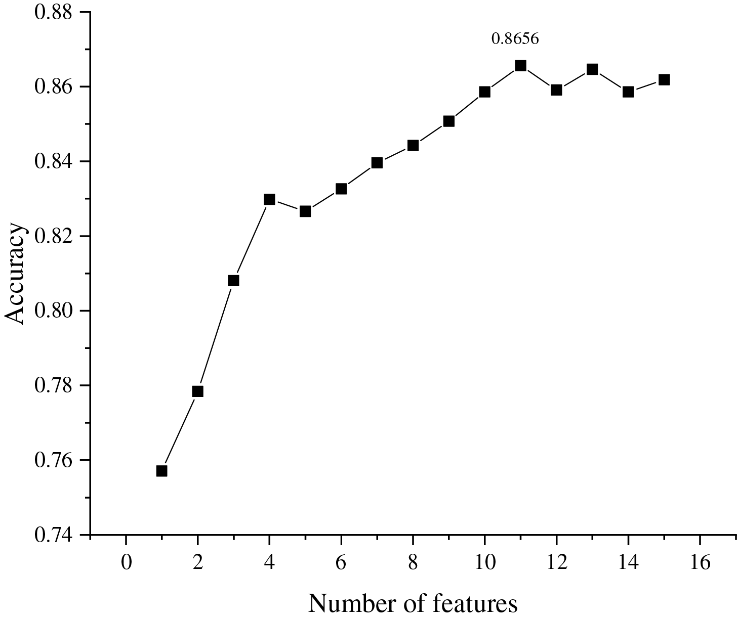
Figure 14: The relationship between number of features and classification assessment indicator

It can be seen from Fig. 14 that the highest values of assessment indicator (0.8656) are obtained when the number of feature subsets is 11. Therefore, the top 11 features are selected as the set of CHD risk indicators, namely: education, age, diaBP, heartRate, prevalentStroke, BPMeds, cigsPerDay, prevalentHyp, sysBP, currentSmoker, diabetes.

4.4.3 Contrastive Analysis

To validate the effectiveness of the proposed method, this subsection compares and analyzes the feature importance scores obtained from the used mRMR, SHAP-RF and ARFS-RF with the multi-angle integrated measurements. The feature importance scores obtained from the above four methods are ranked in descending order, respectively, and the features with the lowest scores are sequentially removed using SBS and input into the LightGBM model for experiments, and the final accuracy variation of the model is obtained as shown in Fig. 15.

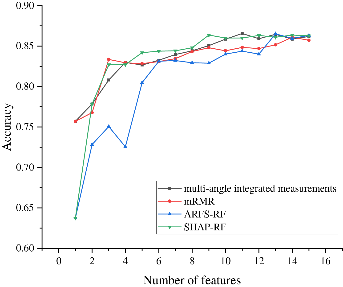
Figure 15: The change curve of accuracy under several different methods

As can be seen from Fig. 15, the accuracy of the LightGBM models all show an increasing trend with the number of selected features, indicating that most of the features are playing a role in the classification model. The multi-angle integrated measurements achieve the highest accuracy when 11 features are selected, which is higher than the highest accuracy achieved by the other three methods. Moreover, mRMR and ARFS-RF retain 14 and 13 features respectively when reaching the highest accuracy. Compared with the proposed method in this paper, the features of the dataset cannot be screened adequately. Although SHAP-RF achieves the highest accuracy when 9 features are retained, its value is still lower than that of the method used in this paper. Therefore, the proposed multi-angle integrated measurements proposed in this paper can fully consider the complex interactions between features and achieve higher classification accuracy when fewer features are retained, which fully demonstrates the effectiveness of the proposed method.

5  Implications for Clinical Practice and Translation to Decision Support

The ultimate goal of identifying key risk indicators for CHD is to translate these findings into practical tools that can aid clinical decision-making. The 11-feature risk assessment system proposed in this study (comprising education, age, diaBP, heartRate, prevalentStroke, BPMeds, cigsPerDay, prevalentHyp, sysBP, currentSmoker, and diabetes) offers a parsimonious yet powerful model for predicting CHD risk.

Our model could be integrated into existing clinical workflows in several ways:

(1) Electronic health record (EHR) embedded risk calculator: A lightweight software tool could be developed to automatically extract these 11 features from a patient’s EHR, calculate their integrated risk score using our LightGBM model, and flag high-risk individuals for further diagnostic testing or preventive intervention. This aligns with global efforts to implement scalable CVD risk assessment tools, such as the WHO’s pocket guide for CVD risk management which also utilizes a concise set of risk factors4.

(2) Point-of-care clinical decision support system (CDSS): The feature set could be incorporated into a mobile or web-based application for use by general practitioners during routine check-ups. Given that our model uses commonly measured clinical and demographic variables (e.g., blood pressure, smoking status, age), it does not require expensive or specialized tests, enhancing its applicability in diverse healthcare settings, including resource-limited environments4.

(3) Patient education and stratification: The risk score generated could serve as a visual aid for physicians to communicate individual risk levels to patients, potentially motivating lifestyle changes (e.g., smoking cessation, blood pressure control). Furthermore, patients could be stratified into different risk categories (e.g., low, medium, high) based on thresholded scores, guiding the intensity of subsequent management strategies, akin to established risk scores like Global Registry of Acute Coronary Events (GRACE) or Thrombolysis In Myocardial Infarction (TIMI) used in coronary syndromes9.

While established scores like Framingham or SCORE provide valuable benchmarks1, our data-driven approach identifies a feature set that includes both traditional (e.g., age, sysBP, diabetes) and less conventional but statistically significant factors (e.g., education level). This may offer a more nuanced risk assessment, particularly for specific populations. The integration of education as a key factor, for instance, could reflect socioeconomic determinants of health, allowing for more personalized risk evaluation.

6  Conclusions

This study proposed a novel hybrid feature selection framework integrating multi-angle measurements and Sequential Backward Selection (SBS) to identify key risk indicators for Coronary Heart Disease (CHD). The most significant results are: (i) Our method successfully identified a concise set of 11 critical risk indicators (education, age, diaBP, heartRate, prevalentStroke, BPMeds, cigsPerDay, prevalentHyp, sysBP, currentSmoker, diabetes) from an initial set of 15 features. (ii) The selected feature subset enabled a LightGBM classifier to achieve a high prediction accuracy of 86.56% for 10-year CHD risk. (iii) The proposed multi-angle integration (mRMR, SHAP-RF, ARFS-RF) demonstrated superior performance compared to using any single method alone, achieving higher accuracy with fewer features, as illustrated in Fig. 15. This validates the effectiveness of combining data-level and algorithm-level perspectives for robust feature selection. Furthermore, our method advances prior work in key areas: Unlike Weng et al. [2] who relied on intrinsic model-based importance, our multi-angle approach offers more robust and interpretable feature ranking. Compared to Wang et al. [8]’s cloud-random forest (which prioritizes prediction accuracy), we emphasize constructing a transparent risk indicator system with only 11 features while maintaining high accuracy (0.8656). Finally, whereas hybrid methods like Nasarian et al. [9]’s 2HFS lack statistical interpretability, our integration of ARFS provides a statistically sound feature importance measure, enhancing credibility for clinical use.

The findings of this study have direct practical implications for clinical practice and medical research: (i) The identified 11-feature system provides a parsimonious and effective tool for clinicians to assess CHD risk rapidly, potentially enabling earlier intervention for high-risk individuals. (ii) The framework emphasizes interpretability. Methods like SHAP provide insights into how each feature contributes to an individual’s risk prediction, fostering trust and understanding among healthcare professionals, which is crucial for the adoption of AI in clinical decision support. (iii) By reducing the number of required indicators, our model can help optimize resource allocation in healthcare settings, focusing on the most informative clinical measurements.

Despite the promising results, this study has several limitations. (i) The analysis relied on a single publicly available dataset from Kaggle. The performance and generalizability of the identified feature set need further validation on larger, multi-center, and more recent clinical cohorts. (ii) The current model provides a static risk assessment. It does not incorporate temporal changes in risk factors, which are inherent in the progression of chronic conditions like CHD. (iii) The framework is built upon specific algorithms (e.g., RF, LightGBM). While effective, exploring other advanced models or deep learning architectures might yield further improvements.

Building upon this research and its limitations, future work will focus on: (i) External validation: Rigorously validating the model on diverse, real-world clinical datasets from multiple institutions to ensure robustness and generalizability. (ii) Dynamic risk modeling: Integrating longitudinal patient data to develop dynamic risk prediction models that can update risk scores based on temporal trends in clinical indicators. (iii) Advanced model exploration: Investigating the integration of more complex models and exploring automated hyperparameter optimization techniques to further enhance predictive performance. (iv) Clinical tool development: Translating this research into a practical Clinical Decision Support System (CDSS) prototype for real-time risk assessment, incorporating user-friendly interfaces and visualization of feature contributions (e.g., SHAP plots). (v) Causal and multi-omics integration: As mentioned in the previous version, exploring causal relationships and integrating multi-omics data remain important long-term goals for a more holistic understanding of CHD.

Acknowledgement: Not applicable.

Funding Statement: This work is supported by the National Natural Science Foundation of China (No. 72071150), and the Fujian Provincial Natural Science Foundation of China (Nos. 2024J01903, 2025J01393).

Author Contributions: The authors confirm contribution to the paper as follows: study conception and design: Hui Qi, Jingyi Lian, and Congjun Rao; data collection: Jingyi Lian; analysis and interpretation of results: Hui Qi and Jingyi Lian; draft manuscript preparation: Jingyi Lian and Congjun Rao. All authors reviewed the results and approved the final version of the manuscript.

Availability of Data and Materials: The datasets generated and analyzed during the current study are available in the [Kaggle site survey report] repository, [https://www.kaggle.com/navink25/framingham] (accessed on 01 September 2025).

Ethics Approval: Not applicable.

Conflicts of Interest: The authors declare no conflicts of interest to report regarding the present study.

References

1. Rao C, Wang J, Liu Y, Yuan J. Risk factor identification mechanism for coronary artery disease based on multiple cross-filtering and binary cuckoo search. Sci Rep. 2025;15(1):32322. doi:10.1038/s41598-025-18024-8. [Google Scholar] [PubMed] [CrossRef]

2. Weng SF, Reps J, Kai J, Garibaldi JM, Qureshi N. Can machine-learning improve cardiovascular risk prediction using routine clinical data? PLoS One. 2017;12(4):e0174944. doi:10.1371/journal.pone.0174944. [Google Scholar] [PubMed] [CrossRef]

3. Xu YB. Risk prediction model and screening model for coronary heart disease [dissertation]. Jinan, China: Shandong University; 2017. [Google Scholar]

4. Rao C, Lian J, Wen J, Chen L. Predicting risk of coronary heart disease using a teaching-learning seagull optimization algorithm with the lightboost based gradient boosting machine. Int J Mach Learn Cybern. 2025:1–20. doi:10.1007/s13042-025-02719-5. [Google Scholar] [CrossRef]

5. Galimberti F, Olmastroni E, Casula M, Xie S, Catapano AL. Contribution and interaction of polygenic predisposition and family history of coronary heart disease in predicting cardiovascular risk. Atherosclerosis. 2025;408(10):120451. doi:10.1016/j.atherosclerosis.2025.120451. [Google Scholar] [PubMed] [CrossRef]

6. Li Y, Wang H, Xiao Y, Yang H, Wang S, Liu L, et al. Lipidomics identified novel cholesterol-independent predictors for risk of incident coronary heart disease: mediation of risk from diabetes and aggravation of risk by ambient air pollution. J Adv Res. 2024;65(21):273–82. doi:10.1016/j.jare.2023.12.009. [Google Scholar] [PubMed] [CrossRef]

7. Rao C, Wei X, Xiao X, Shi Y, Goh M. Oversampling method via adaptive double weights and Gaussian kernel function for the transformation of unbalanced data in risk assessment of cardiovascular disease. Inf Sci. 2024;665(8):120410. doi:10.1016/j.ins.2024.120410. [Google Scholar] [CrossRef]

8. Wang J, Rao C, Goh M, Xiao X. Risk assessment of coronary heart disease based on cloud-random forest. Artif Intell Rev. 2023;56(1):203–32. doi:10.1007/s10462-022-10170-z. [Google Scholar] [CrossRef]

9. Nasarian E, Abdar M, Fahami MA, Alizadehsani R, Hussain S, Basiri ME, et al. Association between work-related features and coronary artery disease: a heterogeneous hybrid feature selection integrated with balancing approach. Pattern Recognit Lett. 2020;133(2):33–40. doi:10.1016/j.patrec.2020.02.010. [Google Scholar] [CrossRef]

10. Zhang Z. Research on key techniques of cardiovascular diseases risk prediction based on machine learning [dissertation]. Chengdu, China: University of Electronic Science and Technology of China; 2021. [Google Scholar]

11. Bilal H, Tian Y, Ali A, Muhammad Y, Yahya A, Abu Izneid B, et al. An intelligent approach for early and accurate predication of cardiac disease using hybrid artificial intelligence techniques. Bioengineering. 2024;11(12):1290. doi:10.3390/bioengineering11121290. [Google Scholar] [PubMed] [CrossRef]

12. Bilal H, Muhammad Y, Ullah I, Garg S, Choi BJ, Hassan MM. Identification and diagnosis of chronic heart disease: a deep learning-based hybrid approach. Alex Eng J. 2025;124(4):470–83. doi:10.1016/j.aej.2025.03.025. [Google Scholar] [CrossRef]

13. Singh A, Nagabhooshanam N, Kumar R, Verma R, Mohanasundaram S, Manjith R, et al. Deep learning based coronary artery disease detection and segmentation using ultrasound imaging with adaptive gated SCNN models. Biomed Signal Process Control. 2025;105(3):107637. doi:10.1016/j.bspc.2025.107637. [Google Scholar] [CrossRef]

14. Boukhamla A, Azizi N, Belhaouari SB, Dey N. Exploring advanced deep learning approaches in cardiac image analysis: a comprehensive review. Comput Biol Med. 2025;196(Pt A):110708. doi:10.1016/j.compbiomed.2025.110708. [Google Scholar] [PubMed] [CrossRef]

15. Kozodoi N, Lessmann S, Papakonstantinou K, Gatsoulis Y, Baesens B. A multi-objective approach for profit-driven feature selection in credit scoring. Decis Support Syst. 2019;120(6):106–17. doi:10.1016/j.dss.2019.03.011. [Google Scholar] [CrossRef]

16. Olawade DB, Soladoye AA, Omodunbi BA, Aderinto N, Adeyanju IA. Comparative analysis of machine learning models for coronary artery disease prediction with optimized feature selection. Int J Cardiol. 2025;436(2):133443. doi:10.1016/j.ijcard.2025.133443. [Google Scholar] [PubMed] [CrossRef]

17. Houssein EH, Hosney ME, Oliva D, Mohamed WM, Hassaballah M. A novel hybrid Harris Hawks optimization and support vector machines for drug design and discovery. Comput Chem Eng. 2020;133(6604):106656. doi:10.1016/j.compchemeng.2019.106656. [Google Scholar] [CrossRef]

18. Hashemi A, Bagher Dowlatshahi M, Nezamabadi-pour H. A Pareto-based ensemble of feature selection algorithms. Expert Syst Appl. 2021;180(5):115130. doi:10.1016/j.eswa.2021.115130. [Google Scholar] [CrossRef]

19. Cai J, Luo J, Wang S, Yang S. Feature selection in machine learning: a new perspective. Neurocomputing. 2018;300:70–9. doi:10.1016/j.neucom.2017.11.077. [Google Scholar] [CrossRef]

20. Li ZS, Liu ZG. Feature selection algorithm based on XGBoost. J Commun. 2019;40(10):101–8. (In Chinese). [Google Scholar]

21. He Y, Zhou J, Lin Y, Zhu T. A class imbalance-aware Relief algorithm for the classification of tumors using microarray gene expression data. Comput Biol Chem. 2019;80(2):121–7. doi:10.1016/j.compbiolchem.2019.03.017. [Google Scholar] [PubMed] [CrossRef]

22. Zhao ZY, Dai YQ. Improved shuffled binary grasshopper optimization feature selection algorithm. J Front Comput Sci Technol. 2021;15(7):1339–49. (In Chinese). [Google Scholar]

23. Kim Y, Hao J, Mallavarapu T, Park J, Kang M. Hi-LASSO: high-dimensional LASSO. IEEE Access. 2019;7:44562–73. doi:10.1109/access.2019.2909071. [Google Scholar] [CrossRef]

24. Jiménez-Cordero A, Morales JM, Pineda S. A novel embedded Min-max approach for feature selection in nonlinear Support Vector Machine classification. Eur J Oper Res. 2021;293(1):24–35. doi:10.1016/j.ejor.2020.12.009. [Google Scholar] [CrossRef]

25. Liu W, Wang J. Recursive elimination–election algorithms for wrapper feature selection. Appl Soft Comput. 2021;113(1–4):107956. doi:10.1016/j.asoc.2021.107956. [Google Scholar] [CrossRef]

26. Rao C, Lin H, Liu M. Design of comprehensive evaluation index system for P2P credit risk of “three rural” borrowers. Soft Comput. 2020;24(15):11493–509. doi:10.1007/s00500-019-04613-z. [Google Scholar] [CrossRef]

27. Wang JJ, Li W. Multi-objective feature selection method based on hybrid MI and PSO algorithm. J Front Comput Sci Technol. 2020;14(1):83–95. (In Chinese). [Google Scholar]

28. Got A, Moussaoui A, Zouache D. Hybrid filter-wrapper feature selection using whale optimization algorithm: a multi-objective approach. Expert Syst Appl. 2021;183:115312. doi:10.1016/j.eswa.2021.115312. [Google Scholar] [CrossRef]

29. Liu Z, Chang B, Cheng F. An interactive filter-wrapper multi-objective evolutionary algorithm for feature selection. Swarm Evol Comput. 2021;65(4):100925. doi:10.1016/j.swevo.2021.100925. [Google Scholar] [CrossRef]

30. Tiwari A, Chaturvedi A. A hybrid feature selection approach based on information theory and dynamic butterfly optimization algorithm for data classification. Expert Syst Appl. 2022;196(3):116621. doi:10.1016/j.eswa.2022.116621. [Google Scholar] [CrossRef]

31. Giannakas F, Troussas C, Voyiatzis I, Sgouropoulou C. A deep learning classification framework for early prediction of team-based academic performance. Appl Soft Comput. 2021;106(3):107355. doi:10.1016/j.asoc.2021.107355. [Google Scholar] [CrossRef]

32. Qi X, Wang S, Fang C, Jia J, Lin L, Yuan T. Machine learning and SHAP value interpretation for predicting comorbidity of cardiovascular disease and cancer with dietary antioxidants. Redox Biol. 2025;79(7):103470. doi:10.1016/j.redox.2024.103470. [Google Scholar] [PubMed] [CrossRef]

33. Hallberg Szabadváry J, Löfström T. Beyond conformal predictors: adaptive Conformal Inference with confidence predictors. Pattern Recognit. 2026;170(3):111999. doi:10.1016/j.patcog.2025.111999. [Google Scholar] [CrossRef]

34. Wang H, Lv B, Yang F, Zheng K, Li X, Hu X. Algorithmic randomness based feature selection for traditional Chinese chronic gastritis diagnosis. Neurocomputing. 2014;140:252–64. doi:10.1016/j.neucom.2014.03.016. [Google Scholar] [CrossRef]

35. Ghasemi P, Lee J. Unsupervised feature selection to identify important ICD-10 and ATC codes for machine learning on a cohort of patients with coronary heart disease: retrospective study. JMIR Med Inform. 2024;12(6):e52896. doi:10.2196/52896. [Google Scholar] [PubMed] [CrossRef]

36. Attia ZI, Kapa S, Lopez-Jimenez F, McKie PM, Ladewig DJ, Satam G, et al. Screening for cardiac contractile dysfunction using an artificial intelligence-enabled electrocardiogram. Nat Med. 2019;25(1):70–4. doi:10.1038/s41591-018-0240-2. [Google Scholar] [PubMed] [CrossRef]

37. Raghunath S, Ulloa Cerna AE, Jing L, vanMaanen DP, Stough J, Hartzel DN, et al. Prediction of mortality from 12-lead electrocardiogram voltage data using a deep neural network. Nat Med. 2020;26(6):886–91. doi:10.1038/s41591-020-0870-z. [Google Scholar] [PubMed] [CrossRef]

38. Poplin R, Varadarajan AV, Blumer K, Liu Y, McConnell MV, Corrado GS, et al. Prediction of cardiovascular risk factors from retinal fundus photographs via deep learning. Nat Biomed Eng. 2018;2(3):158–64. doi:10.1038/s41551-018-0195-0. [Google Scholar] [PubMed] [CrossRef]

39. Zhang P, Zhang Q, Liu J, Wang D, Ye H, Zhang X, et al. Information fusion and feature selection for multi-source data utilizing Dempster-Shafer evidence theory and K-nearest neighbors. Inf Sci. 2025;718(17):122408. doi:10.1016/j.ins.2025.122408. [Google Scholar] [CrossRef]

40. Chawla NV, Bowyer KW, Hall LO, Kegelmeyer WP. SMOTE: synthetic minority over-sampling technique. J Artif Intell Res. 2002;16:321–57. doi:10.1613/jair.953. [Google Scholar] [CrossRef]

41. Peng H, Long F, Ding C. Feature selection based on mutual information criteria of max-dependency, max-relevance, and Min-redundancy. IEEE Trans Pattern Anal Mach Intell. 2005;27(8):1226–38. doi:10.1109/TPAMI.2005.159. [Google Scholar] [PubMed] [CrossRef]

42. Singla P, Garg H, Gagandeep, Pathak A, Singh SP. Privacy Enhancement in Internet of Things (IoT) via mRMR for prevention and avoidance of data leakage. Comput Electr Eng. 2024;116(5):109151. doi:10.1016/j.compeleceng.2024.109151. [Google Scholar] [CrossRef]

43. Wang J, Wei JM, Yang Z, Wang SQ. Feature selection by maximizing independent classification information. IEEE Trans Knowl Data Eng. 2017;29(4):828–41. doi:10.1109/TKDE.2017.2650906. [Google Scholar] [CrossRef]

44. Aghaeipoor F, Javidi MM. A hybrid fuzzy feature selection algorithm for high-dimensional regression problems: an mRMR-based framework. Expert Syst Appl. 2020;162(2–3):113859. doi:10.1016/j.eswa.2020.113859. [Google Scholar] [CrossRef]

45. Breiman L. Random forests. Mach Learn. 2001;45(1):5–32. doi:10.1023/A:1010933404324. [Google Scholar] [CrossRef]

46. Wang HZ, Lv B, Hong YZ. Conformal predictor based syndrome differentiation for traditional Chinese chronic fatigue diagnosis. J Xiamen Univ. 2014;53(1):41–5. (In Chinese). doi:10.6043/j.issn.0438-0479.2014.01.009. [Google Scholar] [CrossRef]

47. Breiman L. Bagging predictors. Mach Learn. 1996;24(2):123–40. doi:10.1007/BF00058655. [Google Scholar] [CrossRef]

48. Nordin N, Zainol Z, Noor MHM, Chan LF. An explainable predictive model for suicide attempt risk using an ensemble learning and Shapley Additive Explanations (SHAP) approach. Asian J Psychiatr. 2023;79(12):103316. doi:10.1016/j.ajp.2022.103316. [Google Scholar] [PubMed] [CrossRef]

49. Gammerman A, Vovk V. Kolmogorov complexity: sources, theory and applications. Comput J. 1999;42(4):252–5. doi:10.1093/comjnl/42.4.252. [Google Scholar] [CrossRef]

50. Vladimir V, Alex G, Glenn S. Algorithmic learning in a random world. Berlin/Heidelberg, Germany: Springer; 2005. [Google Scholar]