
 Submit a Paper
 Propose a Special lssue
 Open Access
ARTICLE

Demographic Heterogeneities in a Stochastic Chikungunya Virus Model with Poisson Random Measures and Near-Optimal Control under Markovian Regime Switching
1 Department of Mathematics, College of Science, King Saud University, P.O. Box 2455, Riyadh, 11451, Saudi Arabia
2 Department of Mathematics, Government College University, Faisalabad, 38000, Pakistan
3 Department of Basic Sciences and Humanities, University of Engineering and Technology Lahore, Faisalabad Campus, Faisalabad, 38000, Pakistan
4 Institute for Advanced Study, Honoring Chen Jian Gong Hangzhou Normal University, Hangzhou, 311121, China
5 Department of Mathematics, Huzhou University, Huzhou, 313000, China
* Corresponding Authors: Yu-Ming Chu. Email: ; Saima Rashid. Email:
(This article belongs to the Special Issue: Recent Developments on Computational Biology-II)
Computer Modeling in Engineering & Sciences 2025, 145(2), 2057-2129. https://doi.org/10.32604/cmes.2025.071629
Received 08 August 2025; Accepted 22 October 2025; Issue published 26 November 2025
 View Full Text
 Download PDF
Abstract
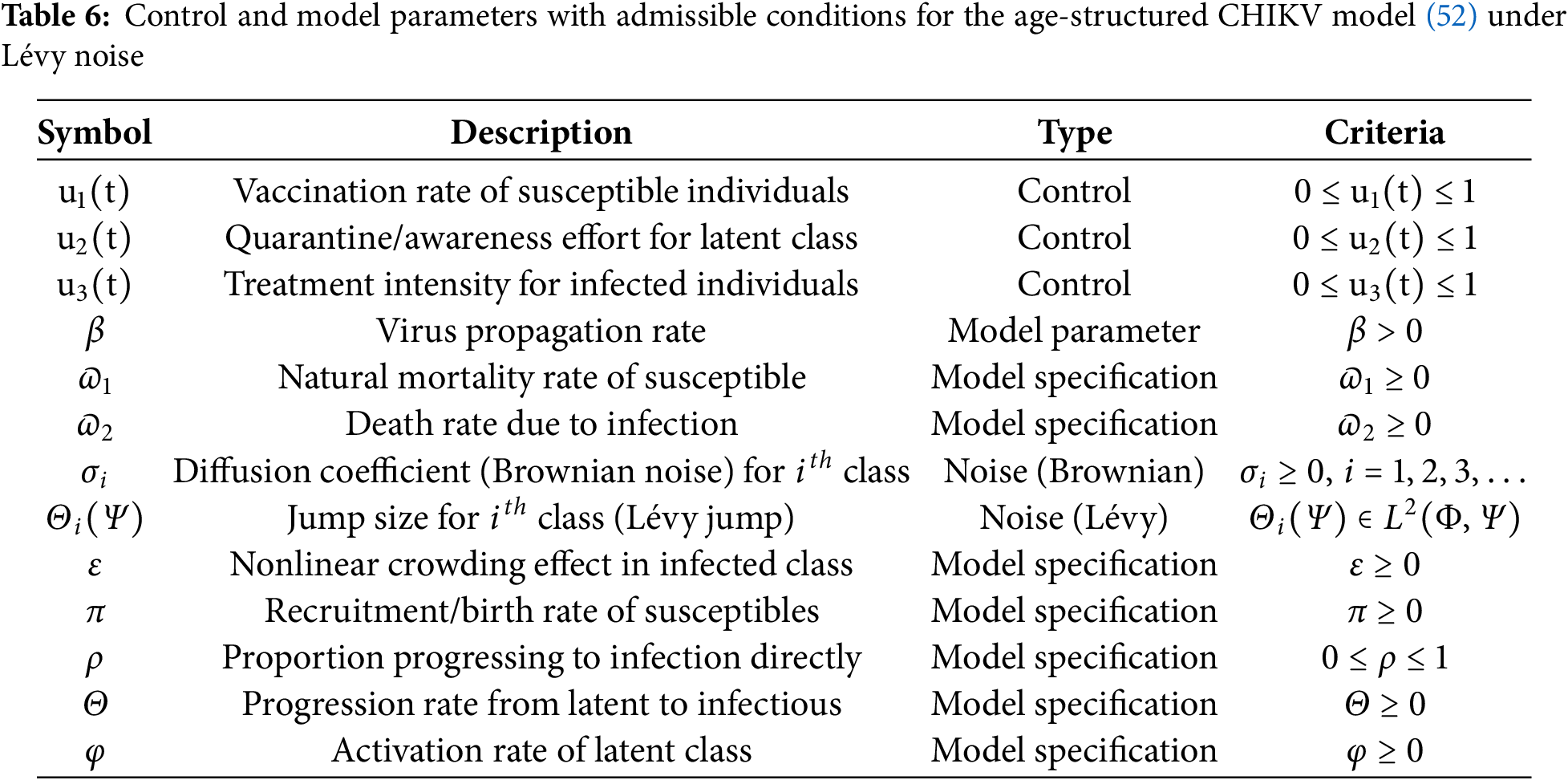
Chikungunya is a mosquito-borne viral infection caused by the chikungunya virus (CHIKV). It is characterized by acute onset of high fever, severe polyarthralgia, myalgia, headache, and maculopapular rash. The virus is rapidly spreading and may establish in new regions where competent mosquito vectors are present. This research analyzes the regulatory dynamics of a stochastic differential equation (SDE) model describing the transmission of the CHIKV, incorporating seasonal variations, immunization efforts, and environmental fluctuations modeled through Poisson random measure noise under demographic heterogeneity. The model guarantees the existence of a global positive solution and demonstrates periodic dynamics driven by environmental factors. A key contribution of this study is the formulation of a stochastic threshold parameter, , which characterizes the conditions for disease persistence or extinction under random environmental influences. Although our analysis highlights age-specific heterogeneities to illustrate differential transmission risks, the framework is general and can incorporate other vulnerable demographic groups, ensuring broader applicability of the results. Using the Monte Carlo Markov Chain (MCMC) method, we estimate = 1.4978 (95% CI: 1.4968–1.5823) based on CHIKV data from Florida, USA, spanning 2005 to 2017, suggesting that the outbreak remains active and requires targeted control strategies. The effectiveness of immunization, screening, and treatment strategies varies depending on the prioritized demographic groups, due to substantial differences in CHIKV incidence across age categories in the USA. Numerical simulations were conducted using the truncated Euler–Maruyama method to robustly capture the stochastic dynamics of CHIKV transmission with Poisson-driven jumps. Employing an iterative approach and assuming mild convexity conditions, we formulated and solved a parameterized near-optimality problem using the Ekeland variational principle. Our findings indicate that vaccination campaigns are significantly more effective when focused on vulnerable adults over the age of 66, as well as individuals aged 21 to 25. Furthermore, enhancements in vaccine efficacy, diagnostic screening, and treatment protocols all contribute substantially to minimizing infection rates compared to current standard approaches. These insights support the development of targeted, age-specific public health interventions that can significantly improve the management and control of future CHIKV outbreaks.
 Keywords
The Aedes mosquito-borne alphavirus (family Togaviridae), known as the CHIKV, has recently resurfaced in several regions worldwide, leading to widespread epidemics. Chikungunya fever is primarily characterized by symptoms such as fever, arthralgia, and, in some cases, a maculopapular rash. Bioactive compounds found in hops (Humulus lupulus, Cannabaceae), particularly acylphloroglucinols—commonly referred to as
Recent outbreaks of CHIKV have been markedly distinct from previous ones, characterized by accelerated transmission and broader geographic spread, often originating in migrant communities from regions where the virus remains endemic. A nationwide epidemic in Malaysia in 1998, primarily driven by workforce migration, exemplifies this trend [3]. Following a 20-year hiatus, Indonesia experienced a significant resurgence from 2001 to 2003 [4]. The 2005 global outbreak in India, affecting 1.4 million individuals, represents one of the most severe in recent history, occurring 32 years after the region’s last major CHIKV event [5]. The national economic impact of this epidemic was estimated at 45.26 disability-adjusted life years per million, approximately equating to 26,000 cases. In 2006, Réunion Island, located southwest of Madagascar in the Indian Ocean, witnessed an epidemic that impacted one-third of its population [6]. This outbreak was particularly severe, with a notably high fatality rate and significant neurological, hepatocellular, and cardiovascular complications. CHIKV, while similar to Zika and dengue, shows distinct clinical features. In endemic areas, 10%–70% are infected and 50%–97% develop symptoms after 4–7 days [7]. Neonates are highly vulnerable, and individuals over 65 have a five-fold higher fatality rate. The disease has an acute phase (7 days) and a persistent/recurrent phase lasting months or years, with acute polyarthralgia affecting 30%–90% of cases; some patients may also experience coronary, neurological, or ocular complications [8]. Chronic CHIKV infection poses ongoing health challenges. During the Réunion Island epidemic, 43%–75% had symptoms one year post-infection, including arthritic pain, fatigue, and neuralgia. Up to 50% may experience persistent pain, often linked to osteoarthritis and ankylosing spondylitis, affecting joints and cartilage [9].
CHIKV transmission occurs in two distinct phases: the forest and city transmission cycles. In the urban cycle, propagation follows a mosquito-mediated human-to-human transmission, while the forest cycle involves a mosquito-borne transmission from animals to humans route [10]. The forest phase is the initial mechanism for the virus’s persistence in Africa [11], whereas the urban cycle dominates in densely populated areas, where Aedes mosquitoes, particularly Aedes aegypti and Aedes albopictus, act as the primary vectors, and humans are the principal hosts [9]. Although Ae. aegypti has traditionally been the dominant vector, the significance of Ae. albopictus has increased, particularly in recent outbreaks in Europe, Gabon, and Réunion [12]. However, as evidenced by the 2013 Caribbean epidemic, Ae. aegypti remains a major vector despite this shift [13]. The spread of Ae. albopictus as a prominent vector has been linked to a genetic variation in the virus’s E1 protein (A226V polymorphism), which enhances the virus’s transmissibility to this mosquito species [9]. Additionally, vertical transmission of CHIKV, particularly in cases following the 2005 epidemic, has been observed, though its validity remains debated [14]. This mode of transmission is considered particularly concerning when the mother remains infected in the days following childbirth [9,11,13].
In humans, the transmission process of CHIKV is well understood, with certain cell types exhibiting heightened susceptibility. Human endothelial and epidermal cells, primordial fibroblasts, and monocyte-derived lymphocytes are particularly prone to infection, facilitating viral propagation. Conversely, CHIKV replication is generally not supported by major lymphocytes, monocytes, lymphoma cells, monocytoid cells, or dendritic cells derived from monocytes [9]. However, this finding remains contentious, as CHIKV-confirmed fibroblasts have been observed in vivo in virus-contaminated individuals [11]. Following initial infection, the host mounts an immune activation, however the infection subsequently spreads to lymphocytes and circulates through various organs [13]. This parasitic phase, marked by widespread viral dissemination, is when mosquitoes can acquire the virus from infected hosts during feeding, facilitating further transmission.
Several aspects of the immune response to CHIKV remain unresolved. To eliminate the virus, CHIKV activates non-hematopoietic mitochondria, primarily fibroblasts, triggering a type I interferon response at the site of infection [15]. The interferon response is regulated by factors 3 and 7, which are less effective in older individuals but are crucial for defending against infection in neonates who lack these factors [15]. Brito and Teixeira [16] highlighted that CHIKV-related fatalities were often underreported within healthcare systems, largely due to limited awareness of the virus’s clinical manifestations and complications. This underrecognition is understandable, given that CHIKV had only recently emerged in the Americas. The authors noted that secondary causes of death—such as cardiac, respiratory, or metabolic conditions—were frequently documented without acknowledging CHIKV infection as the primary or contributing factor. In individuals with persistent symptoms, CD4+ T-cells are more prevalent in synovial tissues, while CD8+ T-cells are found in the skin during the critical phase of the illness [16]. In addition, bone marrow mesenchymal antigen-2 may help mitigate autoimmune responses triggered by CHIKV and protect lymphoid tissue from damage [17].
To better understand biophysical phenomena and the unpredictable nature of transmission of infections, mathematical models have been extensively used [18,19]. Additionally, they are essential instruments for assessing and choosing the best means of control [20]. Sir Ronald Ross’s groundbreaking research on plasmodium established the groundwork for viral infection modeling. Plenty of models have been created since then. Deterministic ordinary differential equations (ODEs) were commonly employed for initial simulations, which assumed consistent death rates and ignored the effects of demographic characteristics and density of the population on morbidity. In [21], Bellan showed that the consequences of vector prevention techniques might be greatly overestimated if age-independent morbidity is assumed. The propagation of many ailments, such as dengue fever, human liver, tumor cells in immunogenetic tumour, HIV with CD4+ t-cells, SARS (severe acute respiratory syndrome), Zika virus, and, most recently, Nipah virus, is also known to be significantly impacted by density of population [18,20]. Recently, Olayiwola and Oluwafemi [22] modeled Tuberculosis dynamics with awareness and vaccination using the Laplace-Adomian method. Olayiwola et al. [23] studied the impact of booster vaccines on managing a new COVID-19 variant using the Laplace-Adomian decomposition method. Mohamed Ali et al. [24] examined stability criteria and optimal control measures for a fractional-order model of human papillomavirus (HPV) infection and cervical cancer. El-Mesady et al. [25] investigated optimal control strategies to reduce HPV transmission in a fractional-order mathematical model.
Meanwhile, the effects of population density have been incorporated into various simulations of insect-borne disease transmission [20]. In [21], the authors considered density-dependent larval mortality rates, but did not account for density effects on transitions between aquatic developmental stages. Although density-dependent mortality during the aquatic phase was included in the basic model of Aedes aegypti population dynamics proposed in [9], the three distinct aquatic stages were merged into a single class. This simplification poses challenges when assessing the impact of specific vector control strategies, as pharmaceutical treatments may affect eggs and larvae differently [14].
Similarly, although Buonomo [26] incorporated mortality driven by population density in humans and mosquitoes within a malaria transmission model, the model did not differentiate between the various aquatic stages of mosquito development via critical aspect for designing effective mosquito control measures. In the same vein, Chitnis et al. [27] studied the propagation processes of the CHIKV by considering only the egg and larval stages of the mosquito population, modeling the effects of density solely on recruitment rates and developmental progression. However, they did not address the impact of larval density on mortality rates, instead focusing exclusively on density-dependent stage advancement during the aquatic maturation process.
Achieving probabilistic optimal control becomes particularly challenging when strict constraints are present. In simpler cases, it may even be impossible to realize true optimal control due to the inherent unpredictability of the system, as highlighted in certain studies [28]. Nevertheless, even in such complex environments, it is often possible to attain near-optimal solutions for stochastic processes [29]. In many applications—such as economics, technology, and beyond developing near-optimal control strategies within an appropriate framework is crucial for achieving desired outcomes. The growing demand for probabilistic near-optimal control has driven significant advancements in this field, establishing it as a key component of dynamic regulation [28,29].
To address these challenges, researchers have developed controlled frameworks based on continuous-time models and finite-state Markov chains, particularly for systems where stochastic differential equations (SDEs) experience abrupt changes phenomena frequently encountered in fields like financial markets, risk management, and asset allocation [30]. Moreover, necessary conditions for ensuring near-optimal control in such complex systems have been rigorously established [30]. It is also widely recognized that environmental perturbation contributes a crucial role in the spread of viral diseases in real-world settings [31]. Since SDEs can more accurately capture the randomness inherent in infection patterns, simulating epidemic outbreaks within a stochastic framework is considered a more reliable approach. Consequently, numerous studies have explored how external noise influences epidemic dynamics [32]. Dereich et al. [33] investigated the behavior of a multilevel Monte Carlo algorithm within an epidemiological framework where population growth remains stable, independent of disease incidence. Their findings demonstrated that the system sustains at least one robust and favorable recurring pattern, ensuring the persistence of the epidemic in a stable environment.
Beyond white noise, Poisson noise is a critical factor in epidemiological simulations, inducing transitions between distinct environmental states [33,34]. In this work, we account for the influence of Poisson noise [35], which drives regime shifts corresponding to varying environmental conditions. For example, fish population growth rates can differ substantially between dry and wet seasons. These transitions, typically following an exponential waiting time distribution, are characterized by a memoryless property [36].
Inspired by the aforementioned literature, we propose a novel model for CHIKV transmission that incorporates density-dependent mortality rates within the human population. This model is calibrated using demographic data from a major CHIKV outbreak in Florida, USA, through the MCMC method. To more effectively quantify the influence of key parameters, a global sensitivity analysis is conducted, focusing on the primary thresholds that govern the model’s dynamics. Incorporating a Poisson random measure, we extend the model to a stochastic framework that accounts for dual infection dynamics, environmental noise with random jumps, and a saturated transmission rate. This stochastic model establishes sufficient conditions for both the persistence and potential eradication of the virus, offering a robust foundation for analyzing long-term disease behavior under fluctuating environmental conditions. Additionally, we address the near-optimal control problem in random frameworks influenced by Poisson noise and regime-switching, without the restrictive requirement of second-order continuous differentiability in the drift and diffusion coefficients. Necessary and sufficient requirements for achieving near-optimal control strategies—such as targeted vaccination and optimized intervention timing—are derived, demonstrating that any
The organization of the work is as follows: Section 2 introduces our autonomous model, which incorporates the adaptive immune response and latently infected cells, and is then extended to a stochastic CHIKV model involving Gaussian white noise and Poisson random measure. Section 3 focuses on the mathematical analysis of the model in relation to the Poisson random measure. Section 4 presents and analyzes the near-optimality control conditions, including numerical simulations and an efficiency analysis. Section 5 discusses model calibration, population stratification, and the contact matrix for the CHIKV model. Section 6 conducts a sensitivity analysis and further examines the optimal control model, including numerical simulations and supporting arguments. Finally, the paper concludes with a summary in the last section. By rigorously analyzing individual class behaviors and leveraging advanced methodologies like Possion random measure, the entire procedurehas been illustrated in the flowchart presented in Fig. 1.
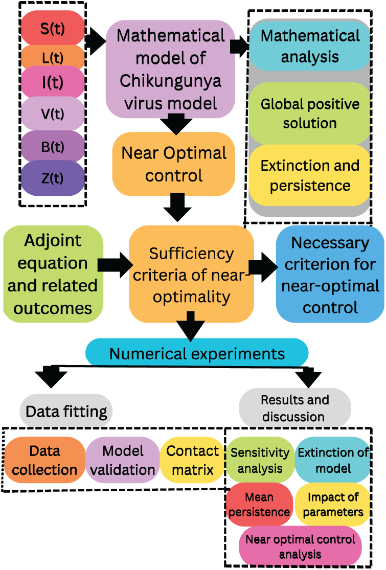
Figure 1: Flow diagram of the overall methodology
In what follows, the development of CHIKV is dependent on the transmission properties of the virus. Chikungunya fever, which is caused by the CHIKV, an alphavirus spread by mosquitoes, is distinguished by an acute fever that appears suddenly, along with eruption, extreme arthritis in the joints, and exhaustion. The Asian continent, the European Union, and the Americas have all seen occurrences of such illness, which is mostly propagated by Aedes aegypti and Aedes albopictus mosquitoes [1,3,4]. Research indicates a clear pattern in the spread of CHIKV [14]. To better understand this phenomenon, we propose two models as follows: Firstly, the interaction between the infectious agent, host cells, and immune components such as T cells and antibodies—is modeled within an adaptive immune response framework for CHIKV. This framework helps explain immune variability during infection and fluctuations in transmission. We proceed by presenting the adaptive immune response model, represented by the following system of ODEs:
subject to the ICs:
(i) The number of sensitive cells,
(ii) Infected cells,
(iii) Infected cells emit
Secondly, by accounting for lymphocytes that have been infected but are not yet infectious, a CHIKV model incorporating latently infected cells offers a more accurate representation of transmission dynamics. This enhancement captures the latent period between viral entry and active replication, improving the precision of predictive algorithms. The incubation phase influences viral propagation potential, timing of immune responses, and viral load buildup. Including this stage strengthens estimates for outbreak control and therapeutic intervention strategies. The following extended framework of ODEs builds upon the previous model by incorporating latently infected cells:
subject to the ICS:
The formulation of the proposed CHIKV models is grounded in established immunological and epidemiological modeling frameworks. The first model (1) focuses on the interaction between susceptible host cells, infected cells, virus particles, and immune responses (T-cells and antibodies). Such compartmental structures have been widely adopted in viral dynamics research (see Shu et al. [37]; Dubey et al. [38]; Handel and Antia [39]) as they capture the essential mechanisms of infection progression and immune regulation.
However, to provide a more realistic description of CHIKV transmission, it is crucial to account for the latent phase of infection, where cells are infected but not yet producing new virions. This motivates the extension presented in (2), where a new compartment for latently infected cells is introduced. Similar extensions have been successfully employed in the study of other mosquito-borne viral infections (see e.g., Buonomo [26], Chitnis et al. [27], Shu et al. [37]; Dubey et al. [38]). Incorporating latency reflects the biological reality that the virus requires an incubation period before active replication, thereby improving predictive accuracy for outbreak size, timing, and intervention strategies.
Thus, the transition from the baseline model (1) to the extended model (2) is justified both biologically and mathematically, ensuring that the formulation aligns with state-of-the-art approaches in infectious disease modeling. This refinement allows the model to better capture observed CHIKV transmission dynamics and provides a more solid foundation for evaluating control measures.
This second model (2) modifies the initial system (1) by incorporating the latently infected cells class
The basic reproductive number
serves as a threshold: if
For the latently infected cells, we have
In spite of the inherent advantages associated with Poisson random measure perturbations, their utility may be further amplified if noise-modulated drift velocity remains inside an optimal threshold domain. The integration of both local and nonlocal Lipschitz criteria underscores that embedding Poisson random measure disturbances can significantly enhance the fidelity and variability of transmitted information, particularly in feedback-driven epidemic models governed by arbitrary SDEs. As highlighted in previous studies [40], Poisson random measure noise exhibits notable advantages over conventional Gaussian disturbances in the context of theoretical epidemiological modeling. Nevertheless, its implementation introduces elevated computational complexity, which poses additional analytical challenges. The jump-diffusion framework incorporating Poisson random measures extends classical formulations by providing a more precise depiction of phenomena such as the abrupt firing of neuronal membrane potentials. Furthermore, the incorporation of such noise mechanisms has been shown to improve the robustness and temporal precision of recurrent neural network (RNN) architectures. When applied to the system described in Eq. (3), the use of Poisson random measure noise leads to a system of compound Poisson-driven SDEs, as detailed in [41].
whereas
A new scheme of the associated SDE model is built to clarify the dynamical interconnections across the CHIKV propagation system, specifically in the occurrence of latently infectious cell compartments. The chronological progression of every demographic compartment with deterministic and stochastic consequences involving Gaussian white noise and Poisson random measure disruptions. Nonlinear prevalence factors control compartment transitions, and stochastic stimuli are included to account for unpredictable interaction occurrences and modifications in the environment. In particular, the abrupt activation of persistent lymphocytes is represented by a Poisson jump mechanism and a delay differential term, which effectively characterize the pattern of latent infections. Transitions such as infection, latency stimulation, virus generation, immune system stimuli, and natural eradication are indicated in the aforementioned system.
However, the compensated Poisson random measure indicated by
The expression
This section presents the foundational definitions and lemmas pertinent to stochastic analysis. The notation and structural conventions adopted here align with those outlined in [42], and will be consistently employed throughout this study.
Lemma 1: ([43]) To facilitate our investigation, we shall employ two essential presumptions, denoted
with
where
Theorem 1: For a stochastic model (4)
Furthermore, if
Thus, the solutions of CHIKV model (4) possess the subsequent features;
Proof: The supporting arguments for this lemma are analogous to those provided for Lemmas 2.1 and 2.2 in [44]; therefore, they are omitted here for brevity in the context of this analysis.
The previously outlined definitions of mean persistence are particularly noteworthy, as highlighted in [42].
Definition 1: ([45])To establish the property of extinction or persistence, the stochastic model (4) is required to satisfy the following conditions:
The criteria outlined herein are consistent with those detailed in [42], wherein the associated lemmas delineate the requisite conditions for the persistence of infection.
Lemma 2: (Strong law) ([45]) Considering a real-continuous mapping
Lemma 3: ([45]) Consider
Therefore, we have
Here,
Definition 2: (Approximate optimal control) ([46]) A set of permissible control strategies
where
The function
If
then
Definition 3: (Generalized gradient in Clarke’s sense) [47] Consider
where
Lemma 4: ([47]) Suppose that
where
Lemma 5: ([47]) Suppose that there is a complete metric space
To enhance the realism of the CHIKV transmission model, we incorporate a compartment for latently infected cells and introduce stochasticity via a Poisson random measure. The resulting stochastic model (4) serves as a physiological analogue for the population dynamics of CHIKV infection. This model formulation requires the presence of a global, bounded, and non-negative solution. To analyze the well-posedness of the system defined by (4), we adopt the standard assumptions
Theorem 2: Surmise that the stochastic model (4), defined for
Proof: Since the drift and diffusion are guaranteed to be locally Lipschitz by the requirement
where
So that, there is a natural number
To demonstrate the remaining part of the hypothesis, we proceed by constructing the mapping as follows:
The aforementioned relationship defines the
Furthermore, (22) ensures the inequality
For a non-negative
By evaluating the integral of both sides of Eq. (26) over the interval from 0 to
Fix
It follows that
Since
This leads to a contradiction, thereby implying that
3 Extinction and Persistence of Disease
In what follows, the criteria for extinction and persistence in the mean are analyzed to better explore the long-term dynamics of the CHIKV system that incorporates inadvertently transmitted viruses and stochastic perturbations controlled by a Poisson random measure. In particular, as time gets closer to infinity, the anticipated outcomes of the resulting constituents are implied to continue to be consistently constrained away from zero by the system’s persistence in mean. On the other hand, disappearance describes the situation in which some compartments, like the transmissible group, asymptotically tend to zero as expected. Using features of the adjusted Poisson integral and stochastic Lyapunov functional components, we obtain sufficient requirements in which the infectious community either dies, disappears, or persists in the mean.
Here, we identify key conditions that favor the eventual eradication of CHIKV within the community. Our primary focus is on the asymptotic behavior of the proposed CHIKV model (4). The analysis begins by formulating a threshold parameter for the system, which serves as a criterion for disease extinction. This threshold provides a quantitative condition under which the infection is expected to die out with high probability. The following result establishes a sufficient criteria for the eradication of the infection in the presence of Poisson random measure:
Theorem 3: Assume that there is a stochastic model (4) possesses the solution
In simple terms, the above result implies that CHIKV will eventually be eradicated from the population with probability one.
Proof: After performing the integration on model (4), the subsequent formulae can simply be generated:
Using the fact of (31), one can easily compute
where
Considering the last formulation of (31), we attain
whereas
implementing Itô’s technique to the infected human population, the third equation of (31) simplifies to the following form:
Applying integration on (36) over
By replacing (32) with (37), we find
Furthermore,
Whenever
Adopting the same technique, we can prove
This yields the intended outcome.
In what follows, we investigate the long-term viability of CHIKV transmission within the general population, specifically under a stochastic framework that incorporates latently infected cells and jump disturbances modeled by a Poisson random measure. To be more precise, we analyze the conditions under which the infection persists, which is a critical prerequisite for designing effective surveillance and control strategies. Our analysis begins with the concept of persistence in the mean, as outlined in [42].
Theorem 4: Assume that the stochastic CHKIV model (4) is perceived as persistent within mean if:
where
and it ensures that the illness will always occur in the community irrespective of
Introducing
Proof: Assume that there are functions
where
Applying the Itô formulation to relation (44), we get
After simplification, we get
For brevity, assume that
Utilizing these
Integrating both sides of the stochastic CHIKV model (4) and replacing (47) into (44), we have
It follows that
Applying strong law defined in Lemma 2, we get
By utilizing Lemma 3, the limit inferior of (48) is provided as:
Likewise,
These outcomes constitute the demonstration of Theorem 4. □
Preventing CHIKV outbreaks presents numerous challenges, particularly when considering complex biological interactions, latent infection phases, environmental variability, and stochastic perturbations induced by Poisson random measures. These sources of uncertainty can substantially alter disease dynamics, potentially leading to unforeseen outbreaks or the resurgence of infections, even in the presence of ongoing treatment and control efforts.
To address these difficulties, researchers have developed near-optimal control strategies that aim to balance the epidemiological goal of minimizing disease prevalence with the economic and logistical constraints associated with interventions such as vaccination, antiviral treatment, and vector control (see [30]). Within this framework, we explore the near-optimality criteria of a stochastic control system modeled by a continuous-time Markov chain, where the evolution of the system is influenced by both continuous fluctuations (e.g., Brownian motion) and discrete, abrupt changes (e.g., Poisson-driven jumps).
This probabilistic modeling approach not only provides a more realistic representation of sudden events—such as mass vaccination campaigns or unexpected environmental changes—but also facilitates the application of stochastic control techniques, particularly through recursive optimization and the Hamilton-Jacobi-Bellman (HJB) framework (see [30]). As a result, it enables the formulation of robust, adaptive intervention policies that perform effectively under uncertainty, offering valuable insights for public health policy, epidemic mitigation, and strategic planning in the context of CHIKV. The system of SDEs under near-optimal control is defined as
Thanks to Kuang et al. [48], we describe the corresponding objective function as:
containing
Lemma 6: Imagine
then
To support the analysis, we introduce the subsequent assumptions:
(
(
(
Remark 1: Under the assertions
Remark 2: For any
4.1 Adjoint Equation and Related Outcomes
Adjoint equations and pretreatment assessments are essential for the analysis and solution of optimal control challenges in stochastic mechanisms, especially those that simulate CHIKV evolution, including inactivated infections and jump dynamics. When processes are affected by stochastic components like Wiener procedures, Poisson random measures, or Markov chains, these methods are essential for determining the factors required for optimality. Adjoint equations, which are frequently expressed as backward SDEs, are essential for describing optimum strategies in the context that the stochastic maximum principle (SMP) offers for these kinds of analysis [30].
Applying jump dynamics through Poisson random effects into CHIKV systems makes it possible for better representation of unexpected alterations in the environment or interventional tactics, including widespread vaccination programs. To investigate fundamental claims, estimations, and categorization of these frameworks, the adjoint formulae obtained within this context are essential. Previous studies have demonstrated their significance (see [30]).
To confirm and strengthen the adjoint equations within the CHIKV model (4), we provide initial findings demonstrating their usefulness and well-posedness. In addition, we present a Hamiltonian function that is specific to our stochastic structure, which sheds light on the changing behavior of the system and makes it easier to derive near-optimal control schemes. In addition to improving our comprehension of infectious processes, this method helps create successful approaches to treatment in the face of ambiguity. Additionally, a Hamiltonian function is introduced for the first time to provide further insights into the dynamics and framework of the problem is stated as:
which is Fréchet differentiable space and linear convexity in the
where
Let
•
•
•
Here, the continuous-time Markov chain
We could also add the subsequent boundary value problems to a backward SDE [48] as it gives a way to derive its first-order adjoint equation. It is more advantageous to portray (52) as
By defining the vector
We introduce the following representation for
The given analysis supports the derivation in [49]. Assuming the validity of assertions
where the multiplicative measure of Lebesgue measure
For a closed convex subset
Theorem 5: It is assumed in the event that the assertions
This theorem is proven using an identical approach to the results established in [50,51], and is therefore omitted for brevity.
Theorem 6: Given that the assertions
Proof: By optimizing and applying integration over
For
Using the fact of [52], we get
As a result of Hölder’s inequality and Cauchy-Schwarz, we get:
Utilizing
In view of (74) and observing Remark 2, we have
Making the use of Bellman-Grönwall inequality, yields
Employing the Cauchy-Schwarz variant, we can conclude that
This finalizes the demonstration.
Theorem 7: Under the hypotheses
Proof: By presupposing the following notations to be used in this section.
The following backward SDE is then satisfied by
with the boundary condition:
The factor
Additionally, by stating a SDE with
where
the solution of (83) can be verified by checking the existence-uniqueness of outcome similar to (73), for
Lemma 4 and the boundedness of
The Bellman-Gronwall variant allows us to write
It is follow that
It is worth-mentioning that
Thus, we have
Consequently, we have
After a straight-forward computation, observe that
Moreover, applying Hölder inequality we have
Utilizing (87) into (93), we attain:
Referring to (94) and observing Remark (59), one can write
Combining (87), (92) and (95), we have
From
It follows that
For
Thanks to
Furthermore, it is straightforward to verify that
By implementing Theorem 5 and putting (100) and (101) into (99), we may achieve
Analogously, we have
The proof that completes the given work can be derived from combining equations (87), (96), (97) and (103).
4.2 Sufficiency Criteria of Near-Optimality
To effectively implement countermeasures against CHIKV outbreaks, it is essential to establish sufficient conditions under which surveillance and intervention strategies achieve near-optimality. This becomes particularly important when accounting for the accelerated transmission dynamics caused by an undetected latent phase and the inherent randomness introduced via Poisson random measures. The inclusion of latently infected compartments introduces additional variability into the system, while Poisson jumps are employed to model abrupt and spontaneous events—such as emergency public health campaigns (e.g., mass vaccination or intensified vector control) or sudden infestations.
However, the system dynamics are governed by a set of SDEs driven jointly by Brownian motion and Poisson random measures, with a cost functional designed to minimize both the disease burden and the cost of interventions over a finite time horizon.
These conditions ensure that, even in the presence of random outbreaks (Poisson perturbations) and latent dynamics, a control strategy—while not exactly optimal—remains effectively close to the optimal policy in terms of cost and outcome. Such frameworks are critical for designing robust intervention strategies that account for delays in infection, stochastic shocks, and cost constraints, ultimately enhancing epidemic preparedness and control for CHIKV.
We now turn our attention to presenting one of the key results of this study: a sufficient condition, as expressed in (52), under which the proposed control qualifies as a stochastic near-optimal strategy.
Theorem 8: Assume that the assertions
consequently, a positive constant
Proof: To begin with, we present the following useful result
It is evident that
According to
Here, operator
and
From this, we deduce that
where
and
Therefore, we have
By leveraging the finding from [46] and utilizing the property that the adapted gradient of a sum is contained within the sum of the adapted gradients, it follows that:
Therefore, it is possible to select
Furthermore, utilizing the aforesaid formulation and the assertion
Since the operator
Taking the expectation on both sides of (118) and merging (109) and (117), we attain
Due to the convexity of the function
Employing Lemma 3.2 from [46], it is straightforward to get
Consequently, from (119)–(121), we deduce that
As
Remark 3: To establish Theorem 8, the function
4.3 Necessary Criterion for Near-Optimal Control
A comprehensive stochastic control strategy is developed by the investigation of the required threshold for near-optimal control of the CHIKV framework (4), which incorporates inadvertent infectious people and is influenced by a Poisson random measure. To precisely represent rapid and unpredictable variations in infectious disease behavior, including unexpected eruptions or interventional impact, this framework employs SDEs featuring jump transitions. In order to minimize a cost criterion that normally weighs operational costs vs. public health objectives, control measures like vaccination or vector elimination are implemented.
Ekeland’s variational concept [46] is used to determine the requirements for near-optimality, guaranteeing the presence of nearly optimal controls and permitting a variational evaluation [53]. As a result, a Hamiltonian function is constructed and adjoint mechanisms are introduced, enabling the formulation of a variational inequality. The main finding is that, in comparison to all other permissible controls, the predicted Hamiltonian under a given condition must be almost maximal—within a small error margin—in order for it to be deemed near-optimal. To operate CHIKV effectively and efficiently in the face of unpredictability, this approach offers essential perspectives.
Here, in order to explain the essential assertions of the near-optimal control problem associated with system (52), it follows that any near-optimal control must satisfy a corresponding necessary maximum principle, with an error of order
Theorem 9: Assume that
Proof: Using the Definition 2, the following can be obtained:
Based on Lemma 4,
For practical purposes, we denote:
which means that:
It is straightforward to demonstrate that
then, we can fix that
It implies that
Considering the concept of the control process
It follows that
Moreover, we have
Consequently, we have
In view of Theorem 7 and the assertion
On the same way, we can derive from assertion
and
So that, combining (136), (137) and (138), we get
Observe that
This completes the proof.
Numerical modeling of CHIKV transmission that incorporates latently infected individuals and Poisson random measures represents a sophisticated approach for understanding the stochastic dynamics of disease spread. In these frameworks, the Poisson random measure accounts for the random occurrence of events—such as sudden outbreaks or control interventions—that influence the dynamics of latent infections.
However, a prominent example is the comprehensive stochastic model developed for CHIKV transmission via Aedes albopictus, which effectively captures both outbreak patterns and suppression strategies. This model demonstrates broader applicability across various nations [1], as it integrates multiple factors including virus strain variation, vector control, and geographic containment measures. The inherent randomness of disease transmission is modeled by treating the number of daily human-vector interactions as a Poisson-distributed random variable. To improve computational efficiency, especially when the average interaction rate is high, a normal approximation is employed for simulating daily contacts.
By simulating the spatiotemporal progression of CHIKV, this approach yields valuable insights into the design and evaluation of intervention strategies. Overall, numerical modeling techniques that incorporate Poisson random measures and other stochastic elements serve as powerful tools for analyzing complex transmission patterns and optimizing control measures under uncertainty.
In order to outline the numerical approach and present the experimental results derived from the implementation of various assertions, a numerical scheme was developed to solve model (4), based on the classical numerical method described in [54]. To efficiently construct the algorithm, we introduced a set of integers,
To generate numerical results for the framework (3), the non-negative preserving truncated Euler-Maruyama (PTEM) technique [55] was employed in conjunction with the previously discussed strategies. The PTEM approach has been widely adopted by researchers for analyzing complex physical processes involving stochastic dynamics [56]. This method was selected for its simplicity and robustness in handling jumps induced by Poisson random measures.
For the model (4), specific parameter configurations were required to quantitatively validate the theoretical findings. Two distinct sets of input parameters, summarized in Section 5.1.2, were employed to simulate the system. Such parametric values also include the initial population sizes of individuals. For each parameter grouping, the framework was modeled over the timeframe
5.1 Fitting CHIKV Data of Florida State, USA
Here, we use the average per month of CHIKV occurrences documented in Florida, USA, between April 2005 and December 2017 to figure out the unidentified characteristics and ICs of system (2). Inadvertently contaminated individuals are taken into consideration in this investigation. The threshold parameter,
5.1.1 Data Collection and Assessment
The Florida Department of Health [57] provided us with confirmed case information covering April 2005 and December 2017 to calibrate a mathematical framework describing the propagation evolution of CHIKV in Florida, USA. The total quantity of documented infections, prevalence rates, and demographic profiles by age and geography are among the many details about CHIKV occurrences documented during the virus’s inception that are included in this repository. The monthly occurrence of cases reported for every demographic is the primary purpose of this investigation. The overall incidence of CHIKV per 100,000 people in diverse generations from April 2005 and December 2017 is shown in Fig. 2a, which accounts for the contribution of inadvertent contracted infections to the evolution of propagation as
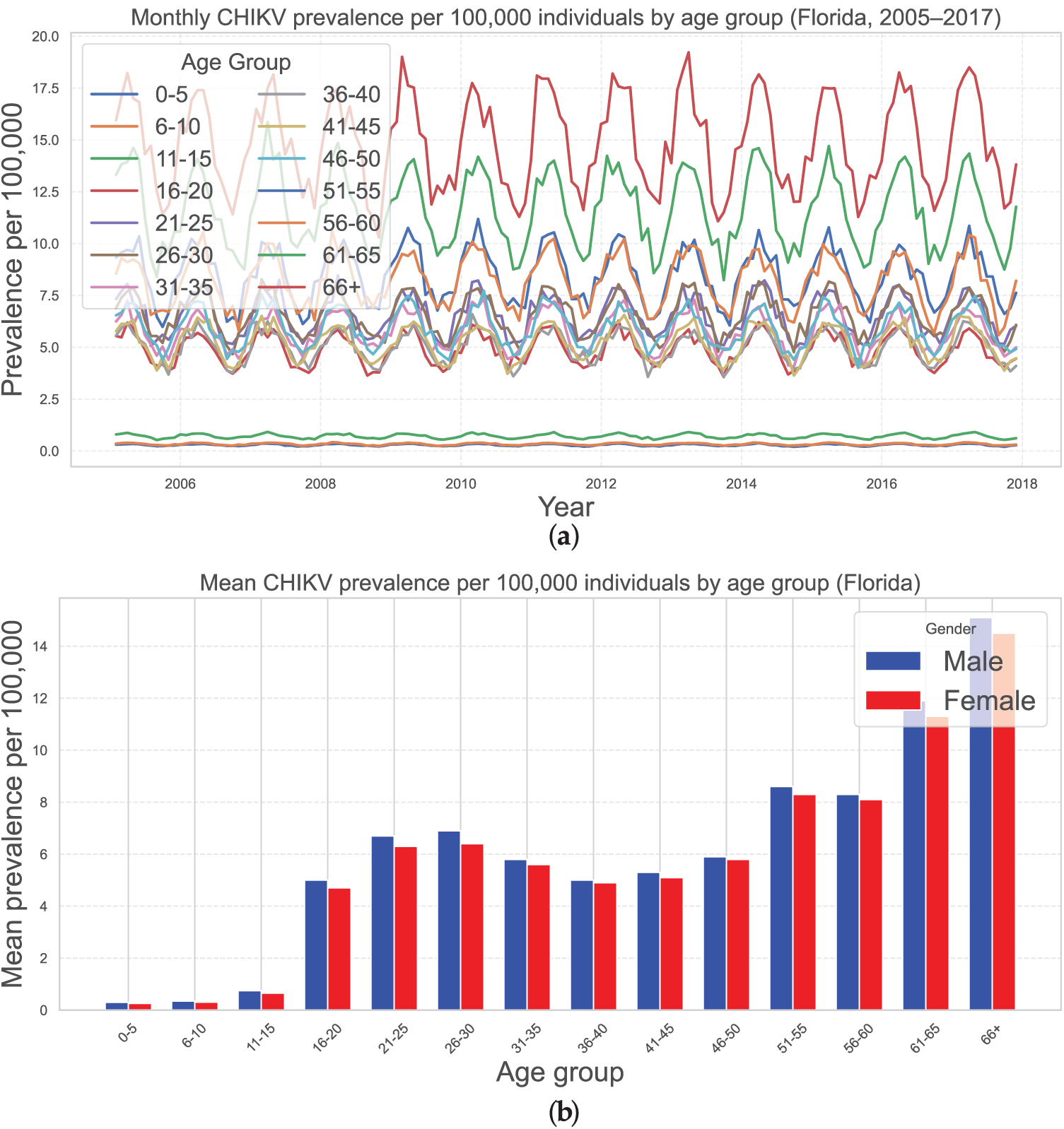
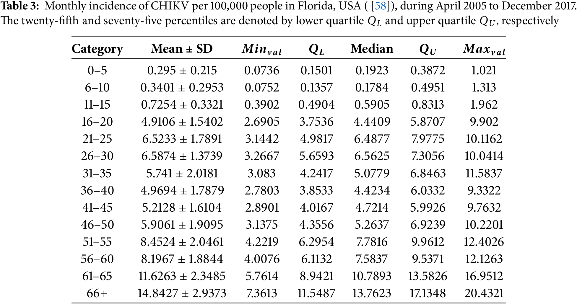
Figure 2: (a) Seasonal fluctuation in the prevalence of CHIKV in Florida, USA, across demographics of people per 100,000 people. Integrating an undetected infection phase inside host cells, the findings illustrate CHIKV characteristics. From early spring through summer, heightened predominance is regularly noted. With an overall mean of 84.2783 instances per 100,000 people, age-dependent average monthly prevalence figures are described, varying from 0.2851 (ages 0–5) to 14.8427 (ages 66+). For a complete quantitative decomposition, see Table 3. (b) Prevalence of CHIKV in Florida, USA, across demographics of people per 100,000 on a gender basis
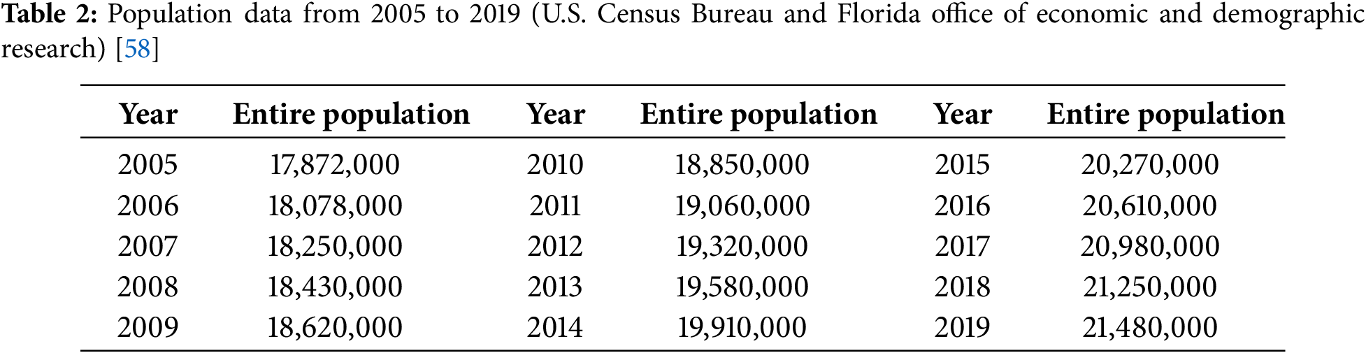
Table 2 displays the aggregate population of Florida from 2005 to 2019, which was gathered according to the Florida Department of Economic and Demographic Research and the U.S. Census Bureau [58]. Fig. 2b displays the 2010 United States Census information for the state of Florida, which includes age and gender-specific demographic profiles.
The frequency of CHIKV per 100,000 people in every demographic varies seasonally, with notable elevations emerging from the beginning of spring to summertime every year, as seen in Fig. 2a. The general population’s estimated monthly CHIKV incidence is 84.2783 cases per 100,000 people. The data shown are age-dependent average recurrence values: 0.2851 for ages 0–5, 0.3288 for ages 6–10, 0.7130 for 11–15, 4.8932 for 16–20, 6.5233 for 21–25, 6.5874 for 26–30, 5.7410 for 31–35, 4.9694 for 36–40, 5.2128 for 41–45, 5.9061 for 46–50, 8.4524 for 51–55, 8.1967 for 56–60, 11.6263 for those 61–65, and 14.8427 for those aged 66 and older (see Table 3). These patterns correspond to the behavior of CHIKV when the host has a latently contaminated lymphocyte component.
The age group under fifteen years old has the lowest frequency of CHIKV, while those over 65 had an elevated incidence per 100,000 people. Furthermore, as illustrated in Fig. 3, Pearson’s correlation assessment demonstrated a substantial positive association between the demographic variability of CHIKV contaminated people from 2005 to 2017 and the overall incidence of CHIKV per 100,000 individuals. In particular, the correlation coefficient between the mean age of CHIKV-infected people and the occurrence of CHIKV per 100,000 people was higher than 0.85 (
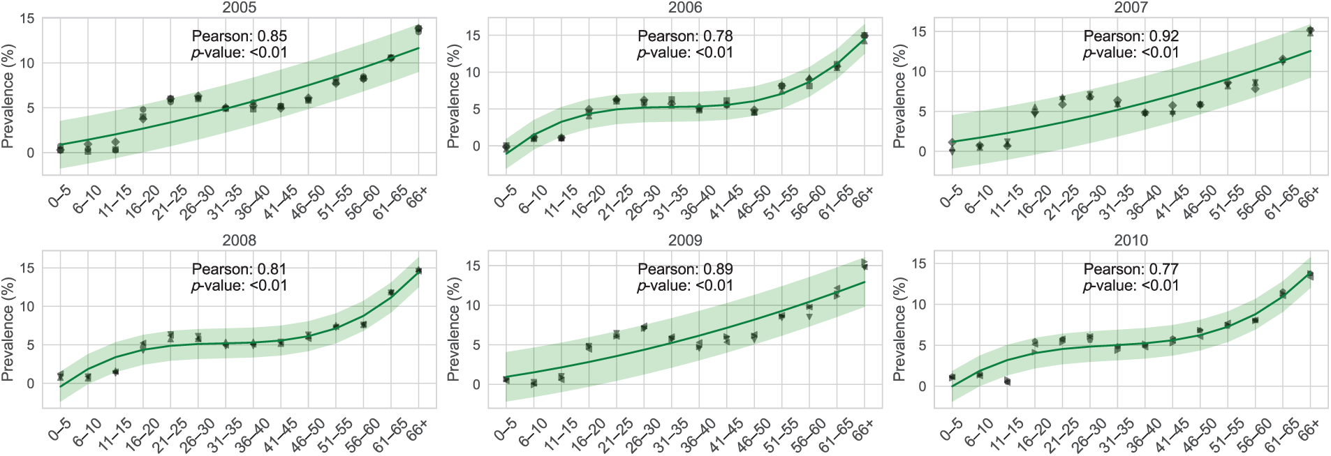
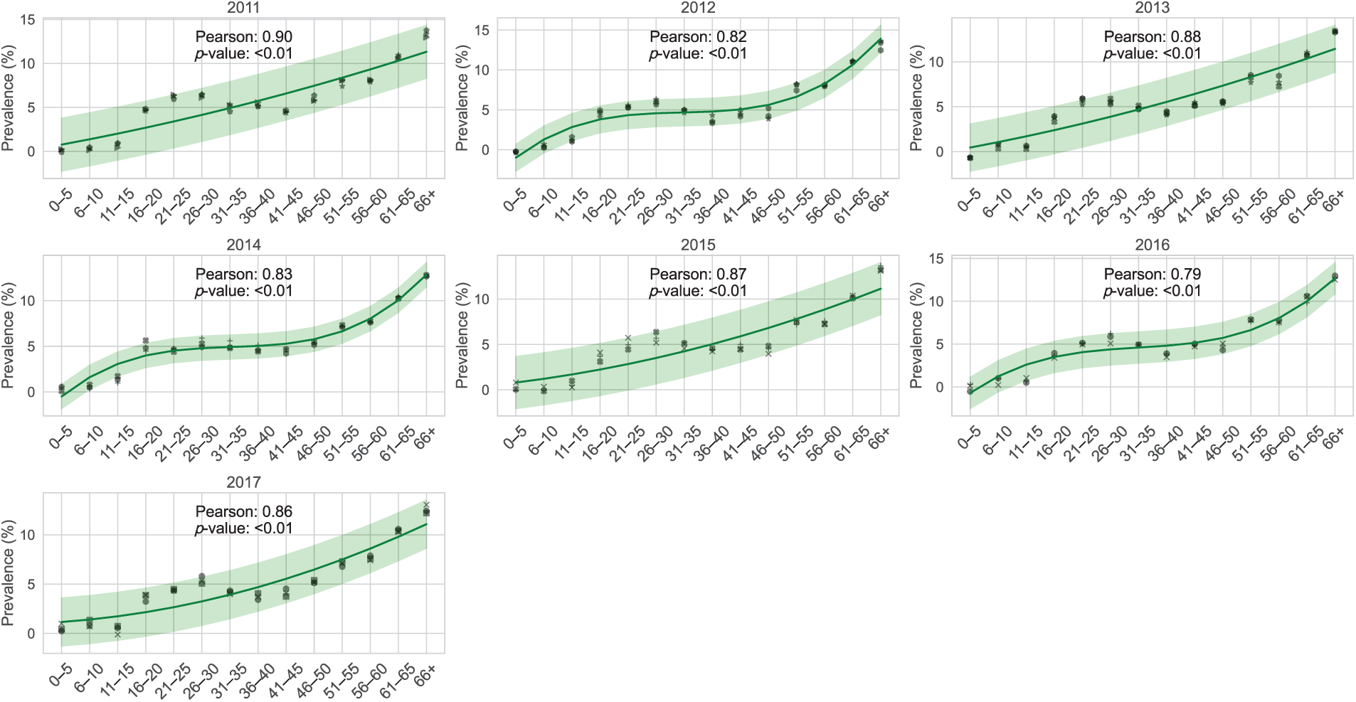
Figure 3: Correlation between age-dependent variations and the prevalence of CHIKV across demographics in Florida, USA, per 100,000 individuals from 2005 to 2017. The prevalence consistently peaks from early spring through summer, with the analysis emphasizing age-specific monthly prevalence, spanning from ages 0–5 to 66 and older
5.1.2 Model Validation and Population Stratification for CHIKV
By analyzing the outcomes of the proposed CHIKV transmission model—which incorporates latently infected cells—against the actual number of confirmed and potential cases, the model’s feasibility is validated. This framework simulates the proportion of potentially acquired CHIKV infections in the state of Florida, USA (see [57]). To ensure realistic and comprehensive simulations, the general population is stratified into 14 age groups, ranging from 0–5 years to 66 years and above. This age-structured approach captures heterogeneous susceptibility, contact patterns, and immune responses across different age cohorts, which is particularly relevant for arboviral infections like CHIKV. Subsequently, all parameters and ICs for the system of ODEs (2) governing CHIKV dynamics are estimated. These estimations incorporate both the demographic characteristics of the population and the host immune response, including the latent phase of cellular infection.
(I) To represent demographic behavior, the general population’s birth rate, denoted by
(II) A typical lifespan in the USA is approximately 76 years, data-driven from the U.S. Census Bureau [58]. Accordingly, natural mortality rates (
(III) According to epidemiological research [59], over 10% of individuals who come into contact with CHIKV and harbor a latent cellular infection eventually develop symptoms during their lifetime. Furthermore, it is estimated that within the first two years after infection, approximately 50% of these symptomatic cases—representing about 5% of all infections—progress to a persistent illness [60]. Consequently, we assume a uniform early progression probability across all age groups and set
(IV) Let
Thus, vaccination reduces vulnerability to successful infection (i.e., development to nonzero
(V) Here,
(VI) The rate at which subconsciously contaminated cells become productively infectious cells is represented by
(VII) The
The monthly likelihood that a CHIKV-latent cellular resource could come back into an active infection in all age categories is represented by such
(VIII) We represent by
We used continuously Morlet wavelet estimation ([63]) to analyze the monthly incidence of cases newly identified in all age categories in order to demonstrate the clear periodicity in CHIKV prevalence. Throughout all 14 communities, the wavelet strength spectrum showed an impressive yearly pattern that was substantial at the 5% level (see Fig. 4a,b). Therefore, we describe
(IX) The total number of people across various age groups is represented as
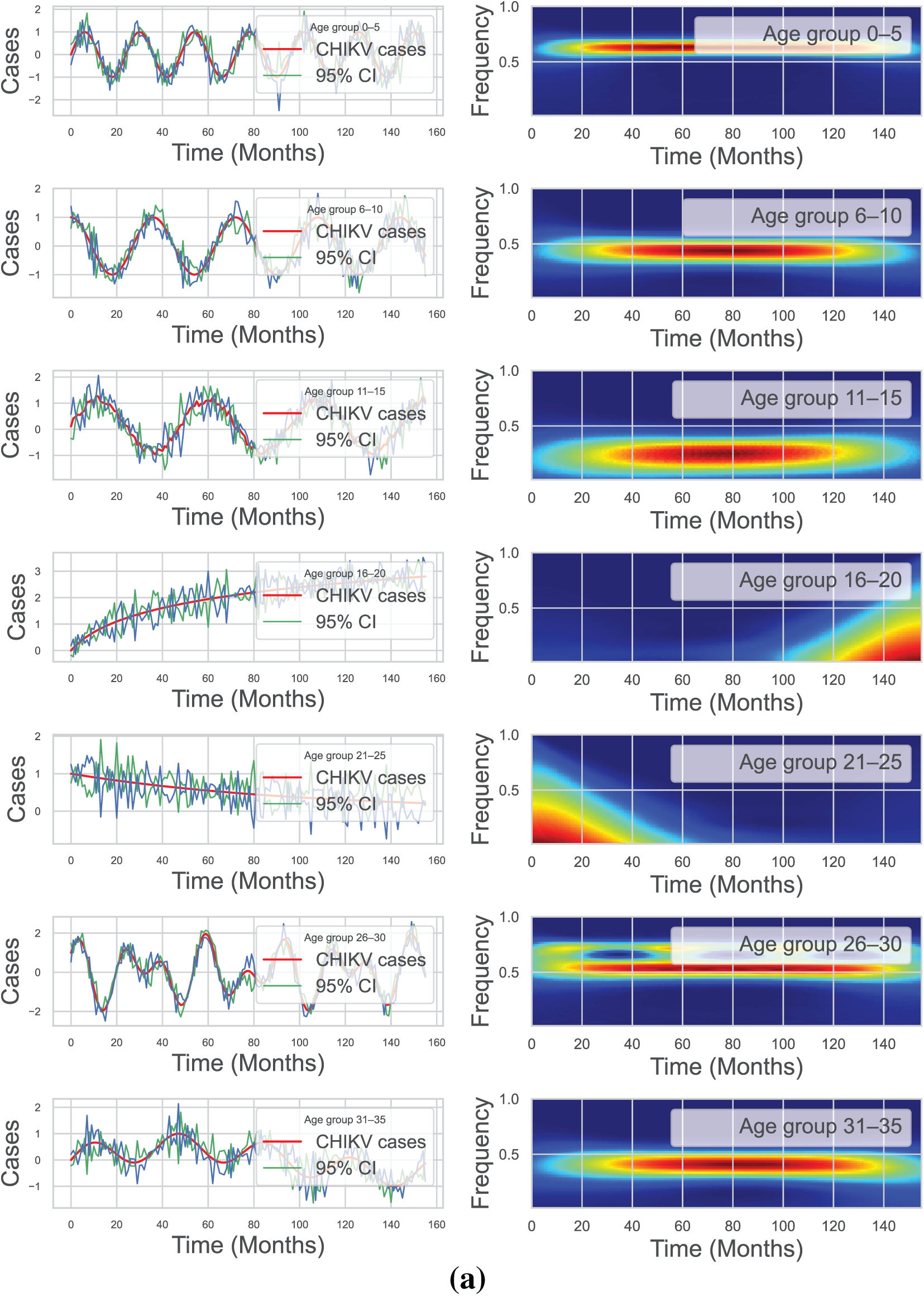
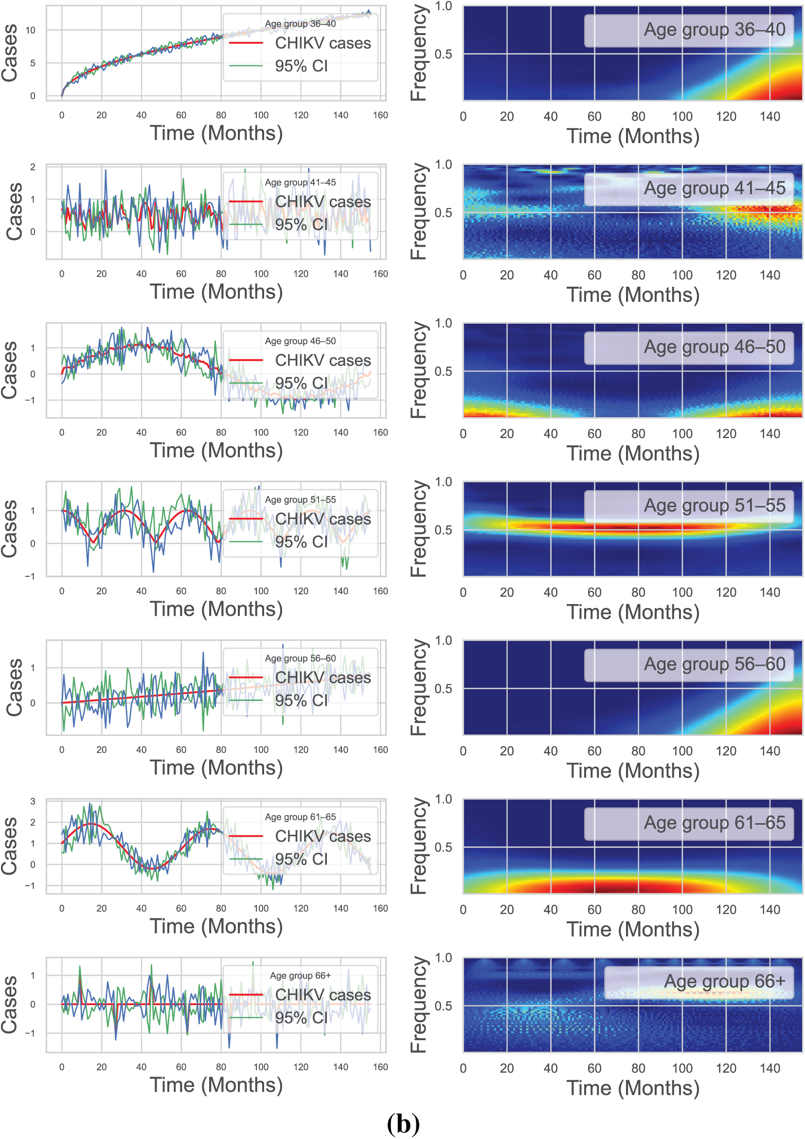
Figure 4: The wavelet method was applied to analyze the spatiotemporal patterns of monthly new CHIKV cases in Florida, USA, across various age groups from April 2005 to December 2017. The first column displays the corresponding 95% confidence curve (green curve) and the average wavelet spectrum (red line). Additionally, the wavelet spectrum analysis of the monthly reported CHIKV cases time series is presented, with low power values depicted in cyan and blue, intermediate power in orange and yellow, and high power in red. The green line represents the 95% C-I
The initial values for the number of infected individuals
According to center of disease control and prevention [64], 90% of newly detected CHIKV cases receive medical treatment. Therefore, the initial number of treated individuals is assumed to be
The initial susceptible population is calculated by subtracting the number of virus concentration, latent, infected, pathogen concentrated, and immune factor from the total population in each age group:
The CHIKV transmission framework with latent infectious cells has been validated through 800,000 repetitions using the MCMC methodology [65], with a burn-in period of 750,000 iterations. We use the recorded monthly prevalence of CHIKV cases as experimental input, considering epidemiological data specific to Florida, USA. These data sets are comparable to those typically used in host-vector interaction studies or more general viral infection modeling approaches. The MCMC procedure captures latent patterns and provides a probabilistic understanding of how well the model fits the observed data, enabling the estimation of unknown parameter values and ICs:
where
Let
Assume that the overall cumulative of infectious people in the
where
where
where
where
Applying a Gaussian deviation approach, the likelihood function
where
The subsequent expression allows for the computation of the prior sum of squares for the supplied components
It is then possible to describe the posterior distribution of factors
The following is a possible expression for the probabilistic ratio required in the Metropolis–Hastings acceptability likelihood:
where the outcome of creating an additional characteristic set is represented by
Unidentified characteristics’ prior understanding is provided by
and a multivariate normal distribution describes the suggested concentration.
Based on epidemiological field data collected in Florida, USA, and as shown in Fig. 5, we fitted the CHIKV model (2)—which incorporates latency and symptomatic stages of infection—using population-level incidence data stratified by age and infection status. This dataset represents the monthly density of infected individuals (per 100,000 population) across structured compartments, including exposed (latently infected), symptomatic, and immune factor cases. The model was calibrated using the MCMC approach, with the final 10% of 50,000 posterior samples employed for statistical inference and parameter estimation.
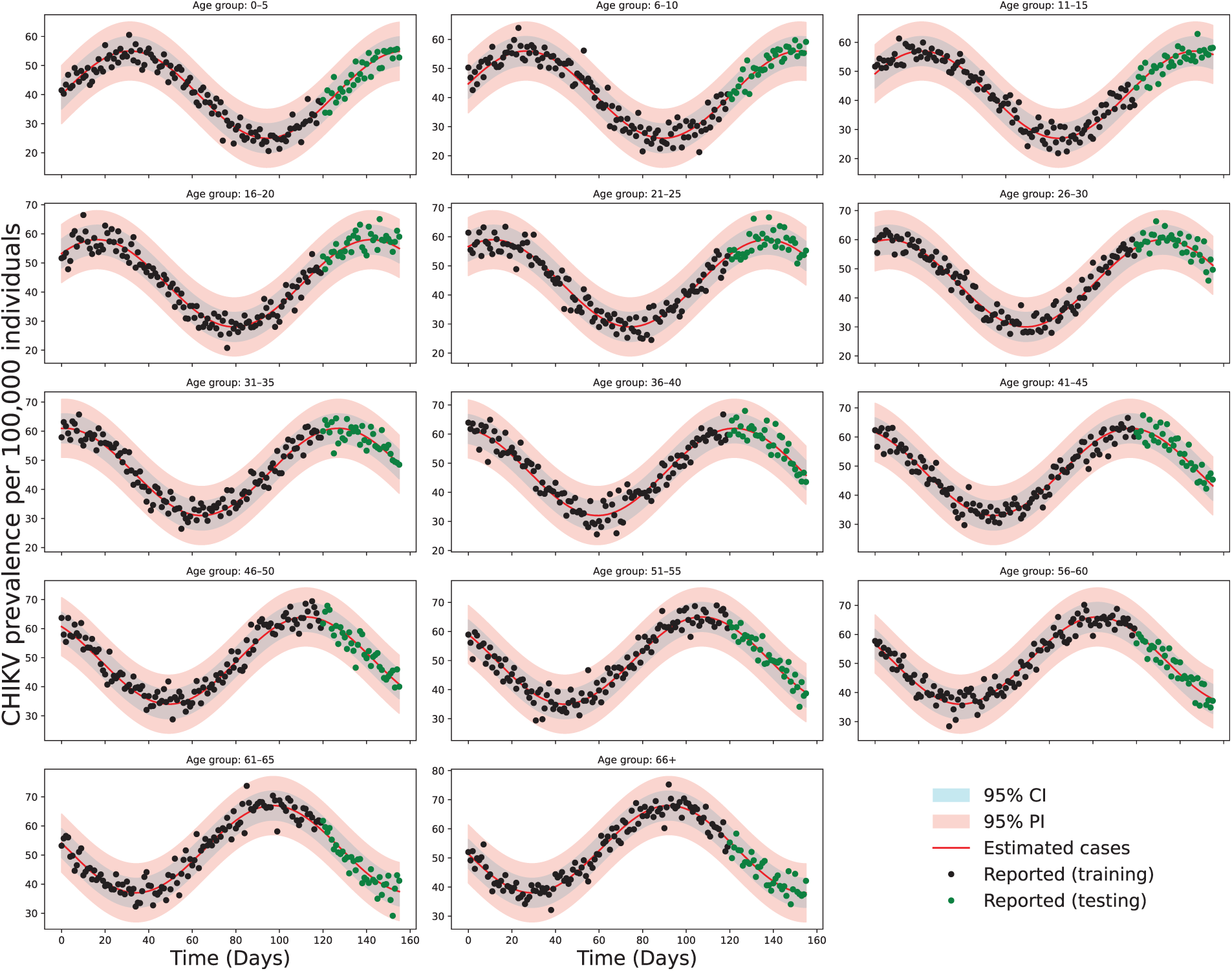
Figure 5: The monthly CHIKV incidence per 100,000 people for various age-factors from April 2005 to December 2017 is shown in the fitting findings. When model (2) is fitted to the measured time series, the simulated trajectories are shown by the solid red lines. The first 120 months of training data are represented by black circles, while the latter 36 months of testing data are represented by green circles. Whereas the light blue shaded area displays the 95% prediction interval (P-I), the magenta shaded area indicates the 95% C-I. A random 10% selection of the previous 50,000 posterior samples was used to generate the final distribution after parameters were inferred using MCMC
Fig. 5 presents the fitted results across age-stratified population classes, showing close agreement between the observed incidence data and the simulated infected population densities. Surface plots for key parameters and ICs of model (2) were generated through MCMC sampling and are displayed in Fig. 6. The constructed model framework demonstrates robust predictive capabilities under the influence of viral transmission dynamics, including latent progression and symptom development. The ratio of our sample size to the free parameters of the model is 28.8:1 > 10:1 [67].
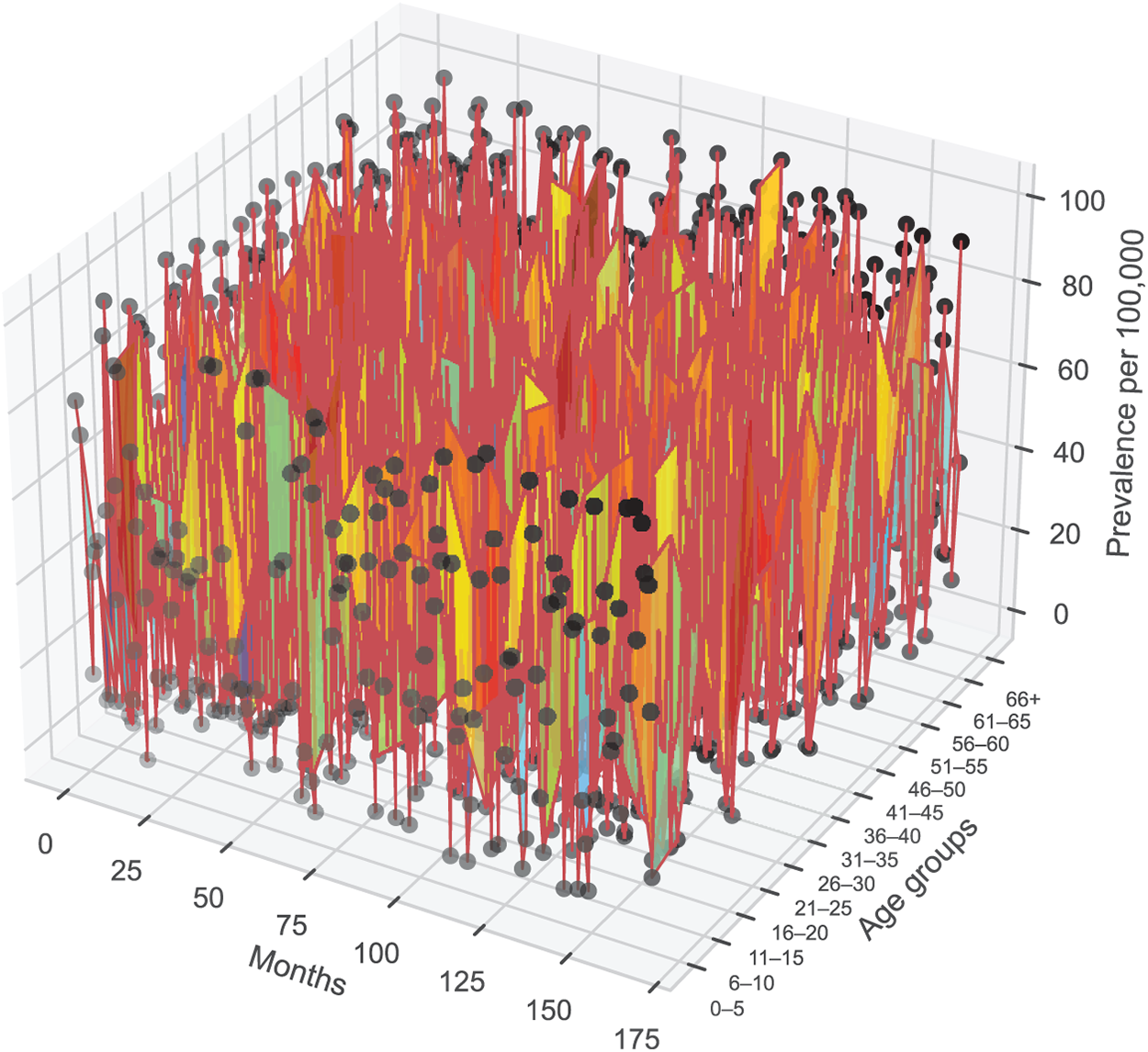
Figure 6: Three-dimensional plot of the predicted outcomes of monthly CHIKV transmission per 100,000 people from April 2005 to December 2017 for various demographic variations. The surface represents the simulated CHIKV prevalence generated from model (2), while black circles correspond to the reported data for each age group over time. CHIKV commonly presents with symptoms such as high fever, severe joint pain, rash, headache, and fatigue, which may vary in severity across different age groups
5.1.3 Contact Matrix for CHIKV Model
Let
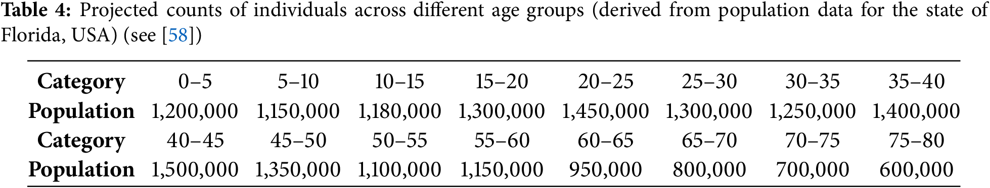
Using Table 4 as a reference, let
To ensure symmetry between
In general, the updated contact matrix constituent can be depicted in the form of:
In this case,
The contact matrix is essential for studying infections such as CHIKV in epidemic modeling, as it quantifies interactions among different age groups. It captures the frequency of interaction involving susceptible people (columns) and infectious people (rows) across various age categories. Understanding these interactions aids in forecasting disease transmission processes, which are influenced by factors such as community behavior and transportation patterns. The matrix, which can be constructed from demographic data, illustrates how different age groups connect—for example, children interacting more frequently with their families (see Fig. 7). It serves a vital function in designing targeted interventions to curb disease spread, like immunization drives or social distancing strategies. Overall, the contact matrix offers vital insights into epidemic dynamics and helps inform effective public health strategies.
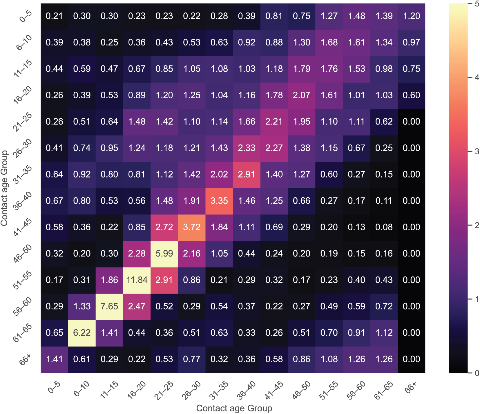
Figure 7: The contact matrix in demographic-structured outbreak models for the propagation of the CHIKV model (2) illustrates how different generations collaborate to forecast transmission and guide focused preventative measures
To analyze the stochastic framework and validate the parameterized model, we conduct numerical simulations of our model (4) in the following section. The objective is to evaluate the effectiveness of coordinated CHIKV prevention and control strategies.
In what follows, the basic reproduction number,
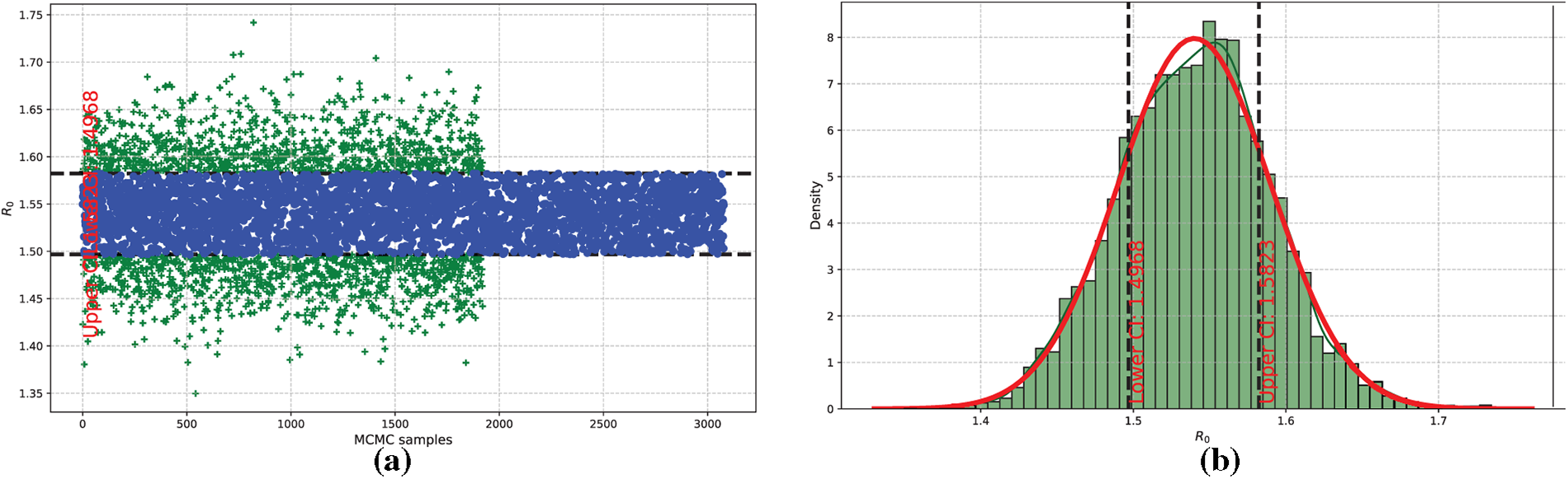
Figure 8: Estimation and distribution of the threshold parameter
Subsequently, we assess the broad dispersion and comparative responsiveness of the parameters incorporated in the CHIKV framework using Latin Hypercube Sampling (LHS) and Partial Rank Correlation Coefficients (PRCCs) (McKay et al. [68]). The aim is to identify the key factors influencing the progression of CHIKV infection. The considered criteria include:
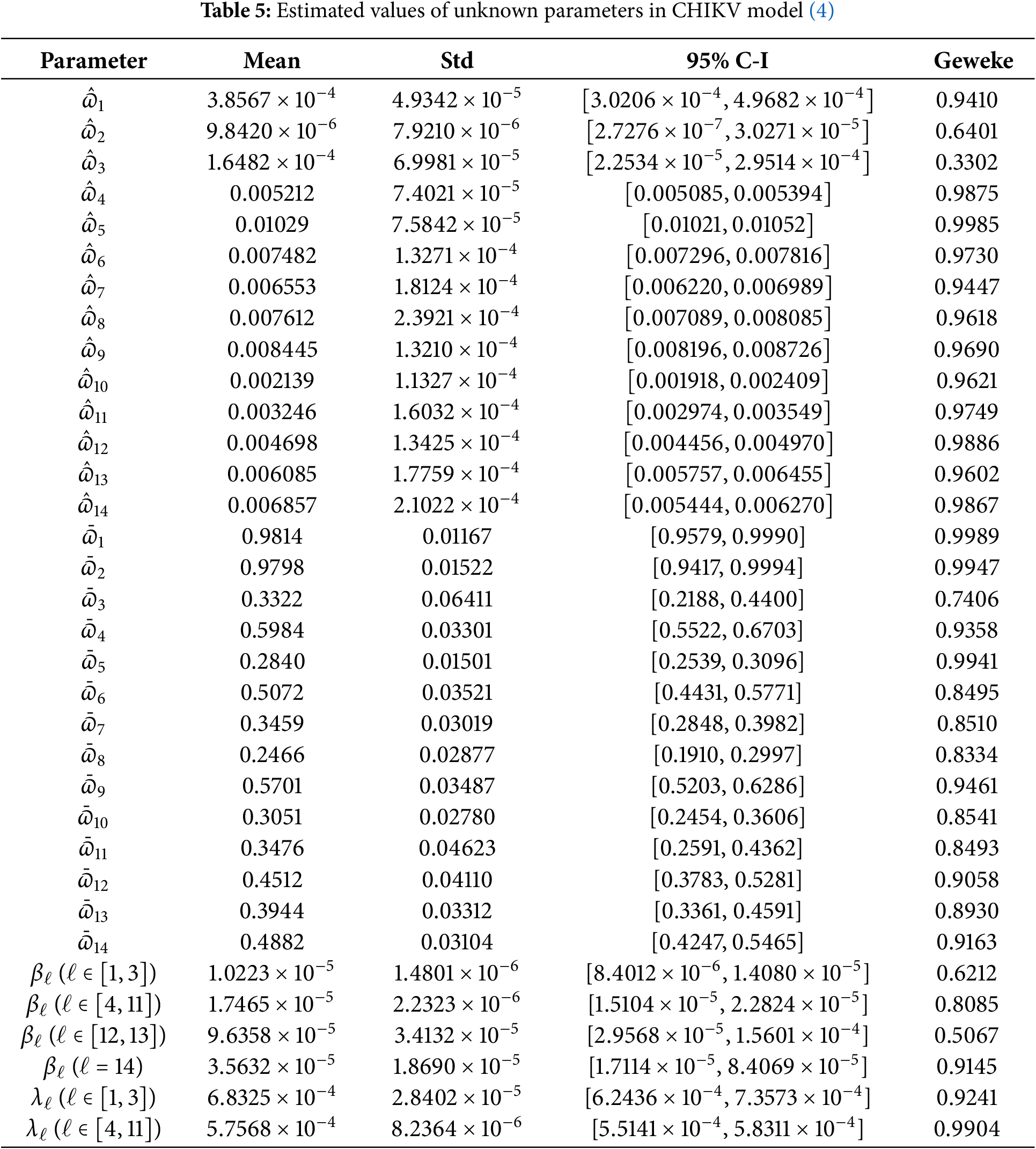
Table 5 presents the sensitivity factors
Further analysis reveals that the risk of reinfection in people harboring latent virus (i.e.,
Lastly,
To comprehensively examine the critical factors contributing to the extinction of the CHIKV (4) in human populations—as well as those facilitating its long-term persistence—we refer to the threshold condition
In this context, virus extinction is primarily driven by stochastic perturbations, natural recovery processes, depletion of infectious reservoirs, increased vector mortality, and the implementation of targeted public health interventions. These include vector control strategies, personal prophylactic measures, and improved environmental hygiene. Even in scenarios with an initially high infection burden, these mechanisms act synergistically to disrupt sustained transmission, ultimately leading to the disappearance of the virus from the host population.
To quantitatively analyze and visualize these findings, we developed a stochastic modeling framework based on Example 1, incorporating random fluctuations to account for real-world uncertainty. Fig. 9 presents numerical simulations illustrating the model’s dynamic progression toward the disease-free equilibrium, consistent with the behavior predicted by the corresponding deterministic system. The resulting stochastic trajectories visibly converge toward the extinction boundary, reinforcing both the biological plausibility of CHIKV eradication under coordinated control efforts and the predictive validity of the proposed framework.
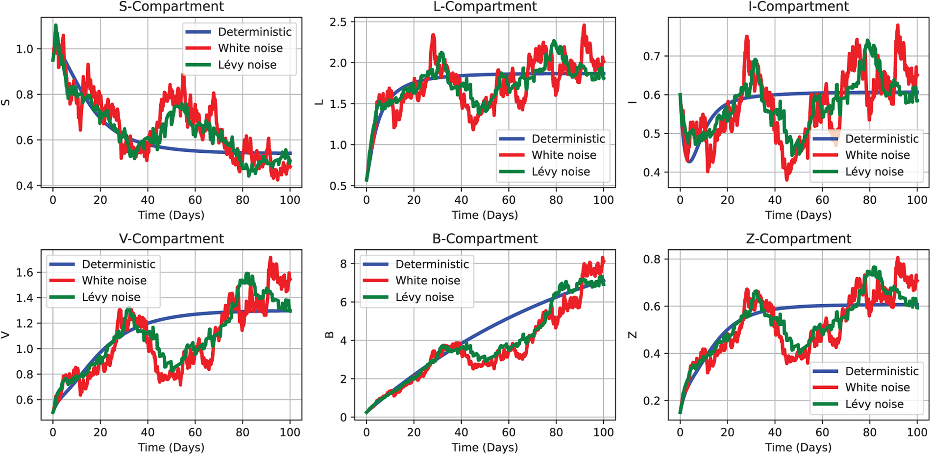
Figure 9: Comparative simulation outcomes of the CHIKV model under deterministic (2), white noise (3), and Lévy noise (4) influences, using the initial parameter values as Test 1 defined in Section 5.1.2. Each subplot depicts the temporal evolution of a distinct compartment—
Example 1: In this scenario, the initial parameter values used for Tests 1, 2, and 3 are presented in Section 5.1.2. These values specify the initial conditions for the susceptible, latent, infectious, vector, and two additional compartments, respectively, reflecting a realistic epidemiological setting. Based on these outcomes, we calculate the appropriate threshold factor
Fig. 9 provides statistical evidence for the gradual eradication of the virus in the general population, as confirmed by these changes. Identical behavioral modeling supporting the extinction outcomes, which are considered reliable, is shown in Fig. 10. This situation exemplifies stochastic extinction, where every solution pathway ultimately leads to the complete elimination of the virus. Notably, this convergence trend remains robust under both stochastic and deterministic influences. Furthermore, the impact of stochastic perturbations on disease progression is highlighted by the faster extinction rates observed in trajectories driven by Poisson random measure noise compared to those influenced by normal jump processes (see Fig. 11).
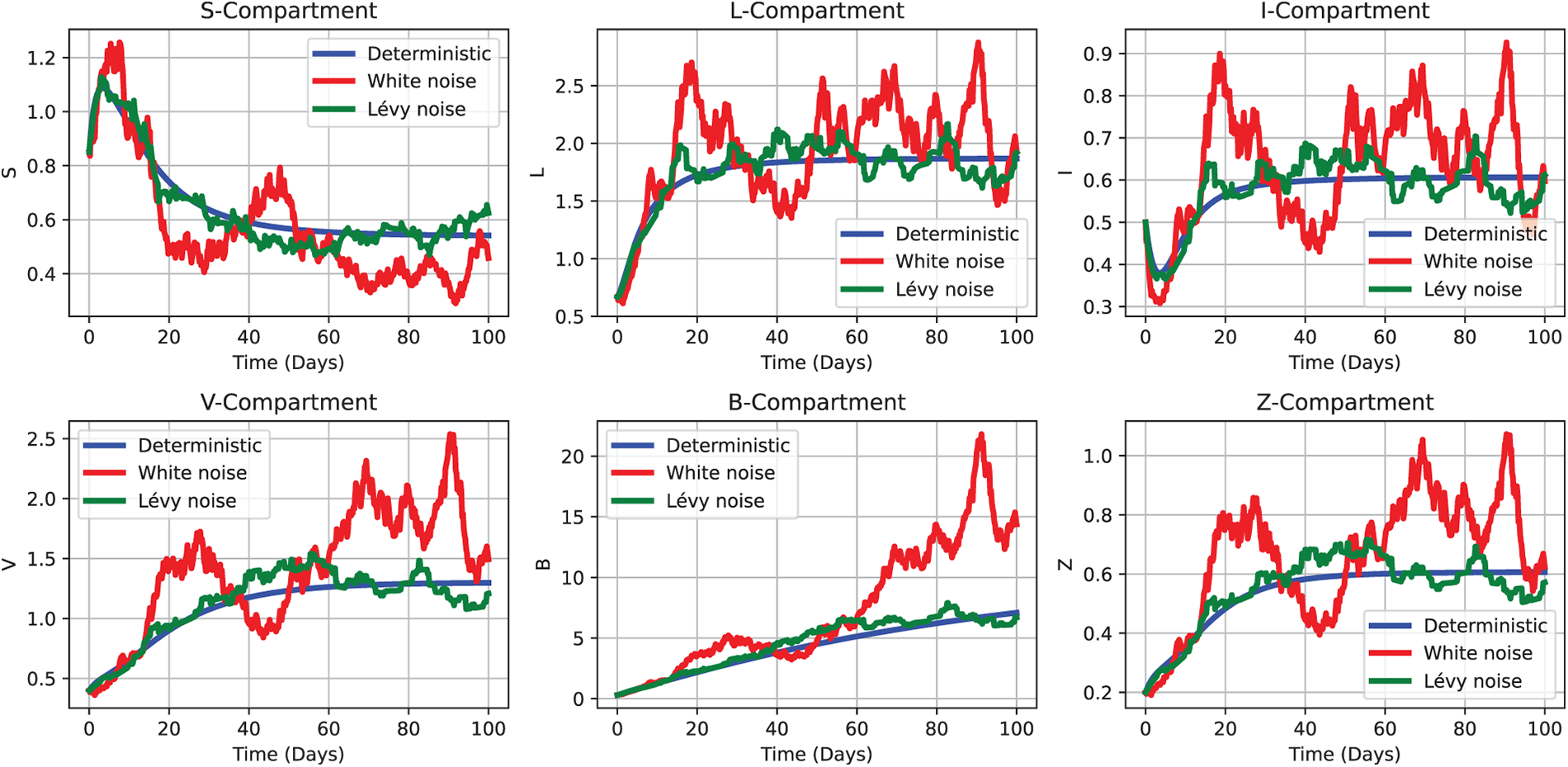
Figure 10: Comparative simulation outcomes of the CHIKV model under deterministic (2), white noise (3), and Lévy noise (4) influences, using the initial parameter values as Test 2 defined in Section 5.1.2. Each subplot depicts the temporal evolution of a distinct compartment—
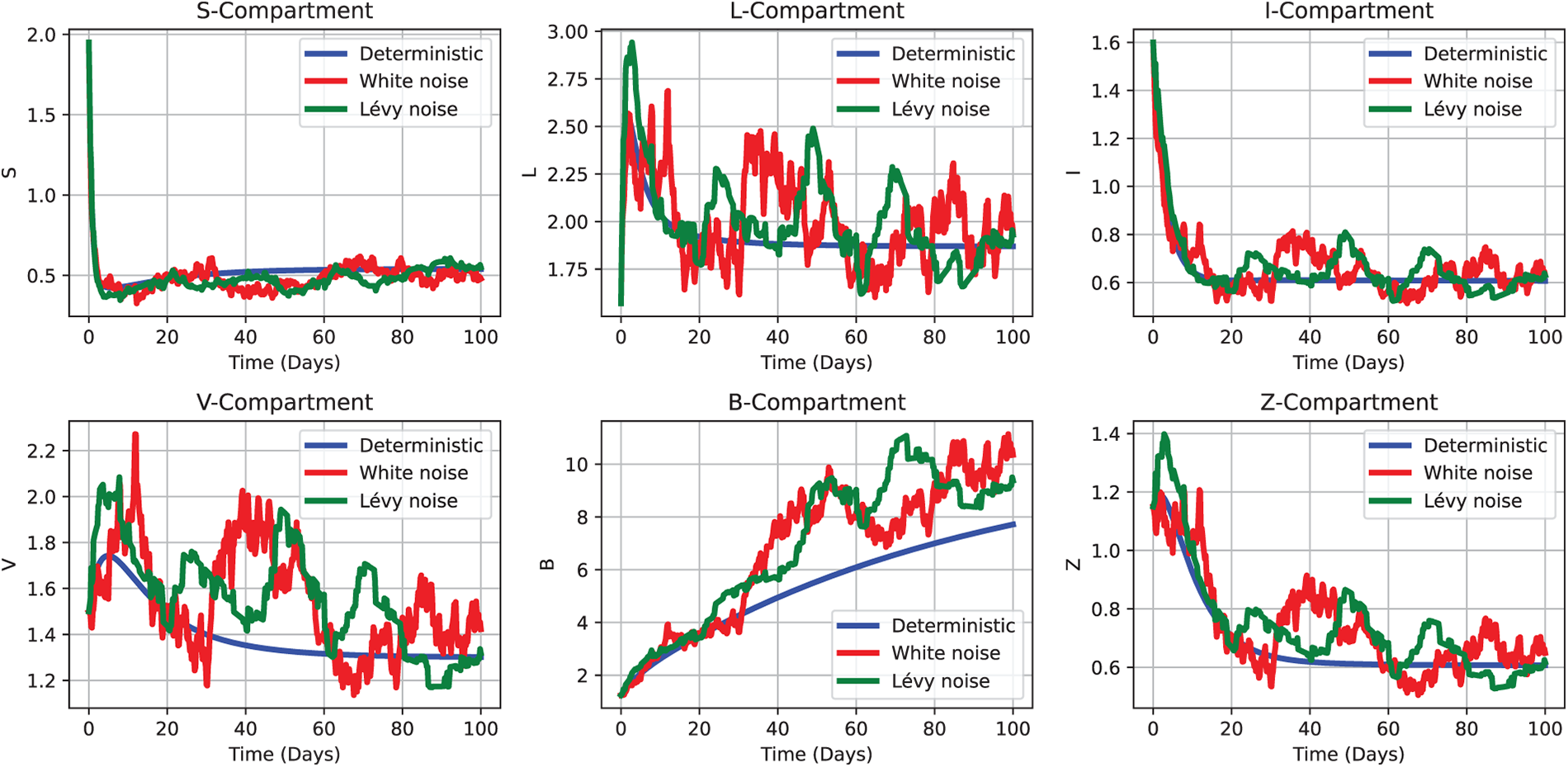
Figure 11: Comparative simulation outcomes of the CHIKV model under deterministic (2), white noise (3), and Lévy noise (4) influences, using the initial parameter values as Test 3 defined in Section 5.1.2. Each subplot depicts the temporal evolution of a distinct compartment—
6.3 Mean Persistence Based Simulation
Focusing on persistence, this investigation evaluates the robustness of a hypothesis concerning CHIKV patterns within a population. Theorem 4 provides the theoretical foundation for understanding the virus’s transmission dynamics, and the results must satisfy its requirements. Section 5.1.2 in Test 2 addresses the case where
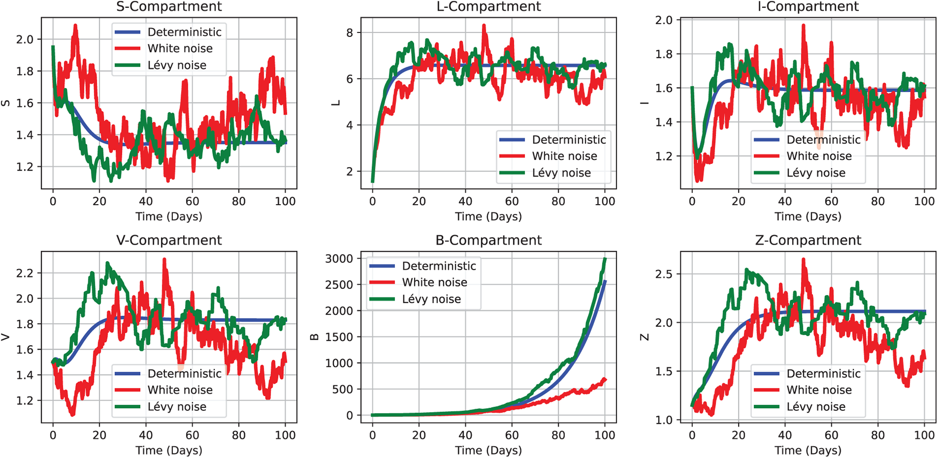
Figure 12: Comparative dynamics of CHIKV transmission under deterministic (2), white noise (3), and Lévy noise (4) frameworks for the case
6.4 Impact of Actively Infected Cells in Concentration
The concentration of actively infected cells, represented by
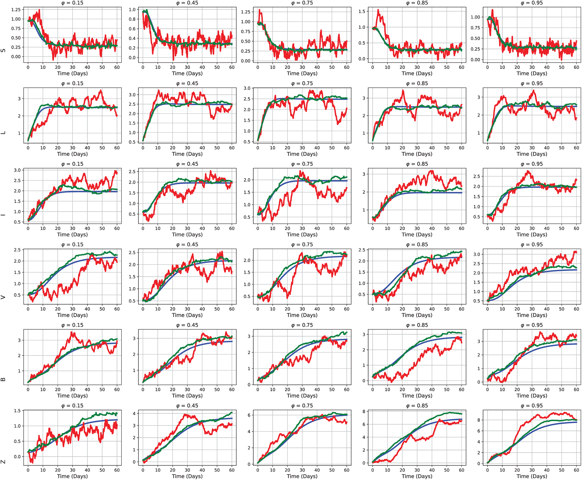
Figure 13: Influence of varying concentrations of actively infected cells
6.5 Impact of
Moreover, the effectiveness of
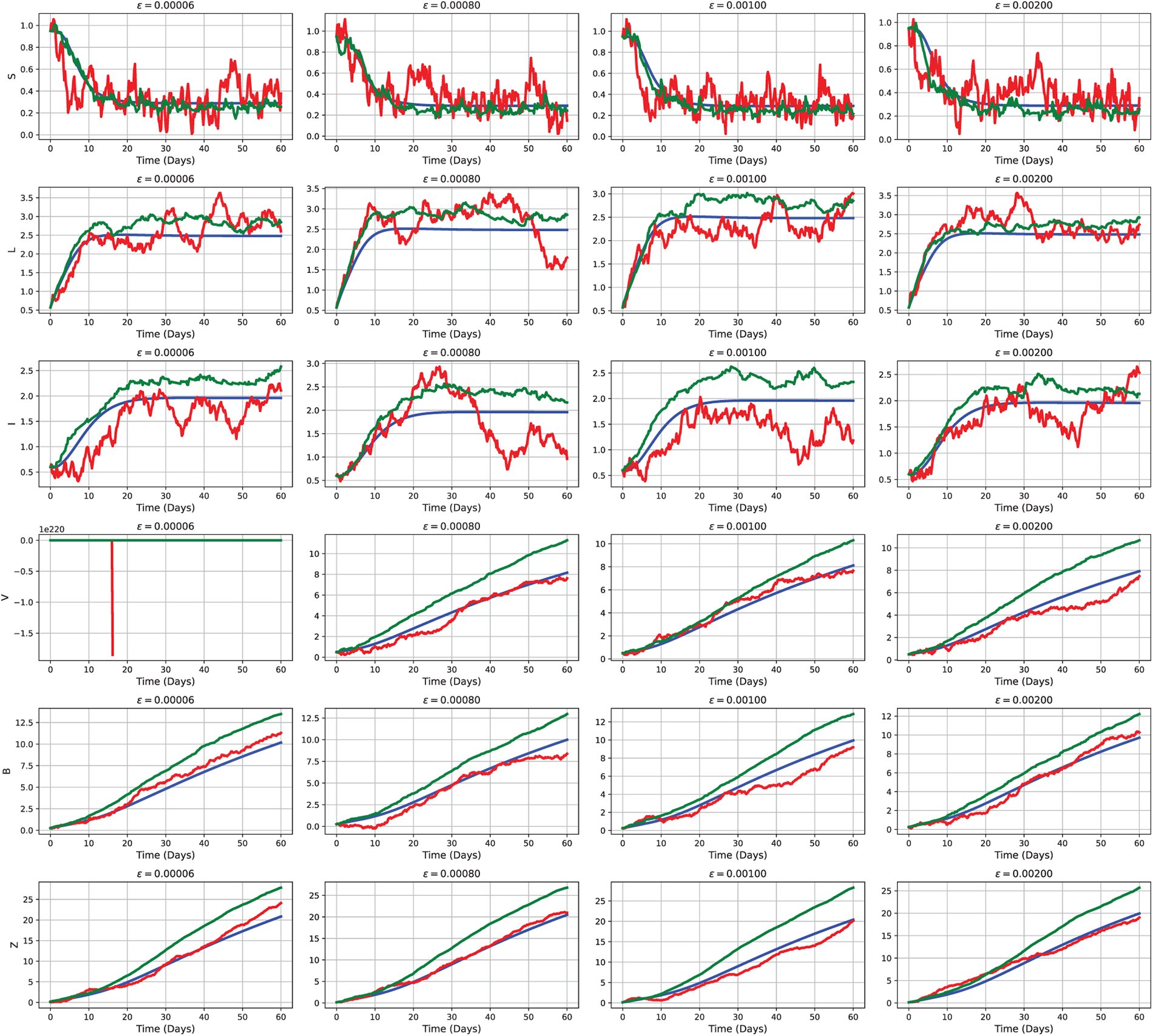
Figure 14: Effectiveness of the CTL cells’ immune response, influence the CHIKV killing rate. A higher
6.6 Near Optimal Control Analysis
A stochastic optimal control approach offers a powerful framework for analyzing the dynamics of CHIKV (52) propagation under the influence of continuous control interventions. This method effectively captures the inherent randomness in disease transmission, which may arise from environmental fluctuations, sudden demographic shifts, or unforeseen outbreaks. To accurately represent such stochastic variability, Poisson random measures are employed. These allow the modeling of discrete jump events within the system, reflecting abrupt and irregular changes such as localized infestations or sudden increases in vector populations [50].
The CHIKV model (52) is typically formulated using a compartmental structure that includes the susceptible, latent, and infectious human populations, along with virus concentration, pathogenic load, and immune response compartments. To represent various intervention strategies, a set of time-dependent control functions is introduced, denoted as
SDEs with jump terms are used to illustrate the system. A Poisson random measure, which introduces unpredictability through discrete, occasional events, governs these jumps. Mathematically, both continuous fluctuations (represented by Brownian motion) and sudden shifts (represented by jumps) affect the evolution of a state variable, such as the pathogenic population
The deterministic component of the dynamics is represented by
The goal of the control approach is to achieve equilibrium between the economic cost of treatments and the impact of illnesses by minimizing a cost functional over a finite time horizon
The weights
Exact control is often unattainable due to the challenges posed by randomness and jumps. As a result, computational techniques such as adaptive programming, Pontryagin’s Maximum Principle in stochastic environments [69], or reinforcement learning-inspired approaches are employed to identify near-optimal control strategies. These methods allow for the dynamic adaptation of control strategies to prevent CHIKV spread, responding to observable situations and jump events.
The following is a detailed algorithm for implementing near-optimal control of the CHIKV epidemic model, governed by a SDE with Poisson random measures. This algorithm utilizes stochastic simulation with control approximation, often through the stochastic maximum principle or dynamic programming combined with MCMC-based backward-forward sweep methods. The Hamiltonian
where
• Initialize control variables
• For each iteration
• Simulate the state equations
• Solve the backward BSDEs for adjoint variables
• Hamiltonian Minimization: Update control
• Check for convergence: if
• Final control
This formulation allows us to analyze and optimize the trade-off between reducing the number of infections and the expense of applying interventions [50].
6.7 Parameter Selection and Simulation Setup
The weight parameters in the objective functional are set as
This study investigates the impact of time-dependent near-optimal control strategies within a stochastic epidemic model comprising multiple compartments. The interactions among these compartments are shaped by persistent infection dynamics, vaccination interventions, and random disturbances in transmission. To account for external uncertainties—such as environmental variability and individual behavioral changes—a Poisson random measure is incorporated into the model, effectively simulating stochastic fluctuations in disease spread.
The assessment of age-structured near-optimal strategies for mitigating CHIKV recurrence under stochastic influences is facilitated by this framework. It explicitly incorporates age-dependent interactions among susceptible, latent, and infectious individuals within each stratification category. These dynamics are influenced by behavioral patterns, vaccination policies, and external disturbances modeled via a Poisson random measure.
As illustrated in Fig. 15, targeted control measures significantly enhance the stability of the susceptible population
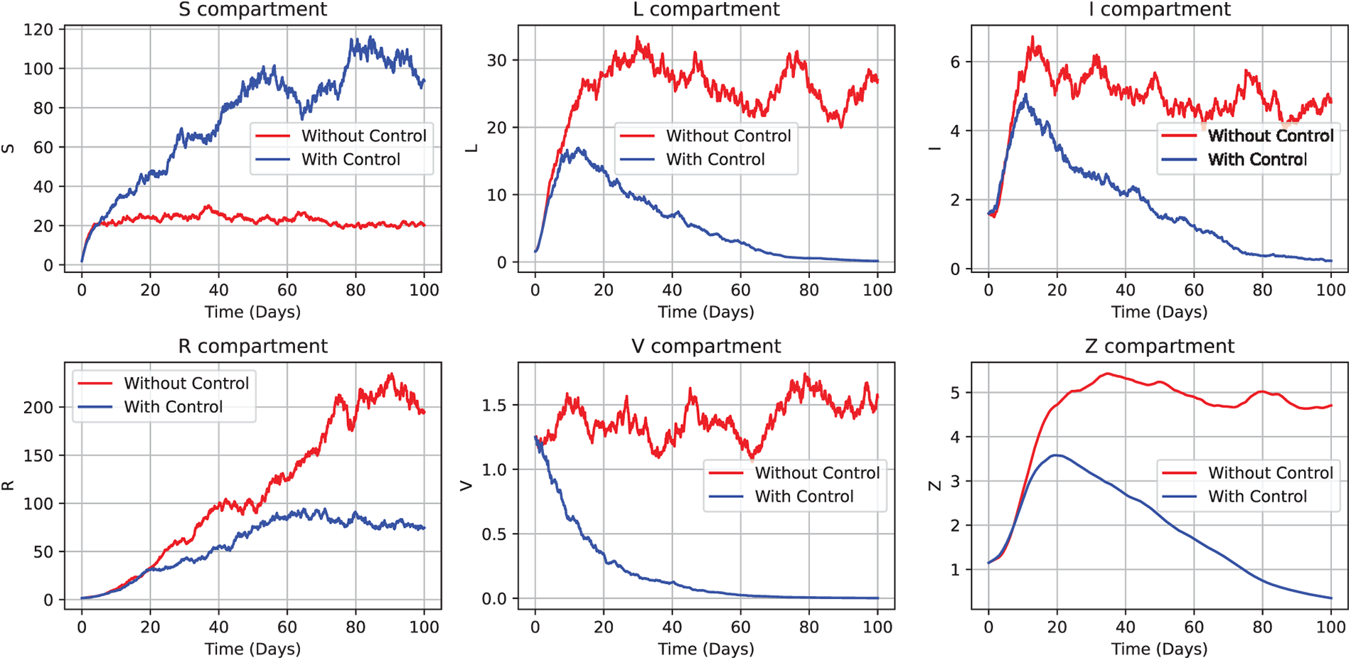
Figure 15: Impact of age-targeted control strategies on the CHIKV model (52). The plot demonstrates that in the presence of optimal interventions,
Theorem 5 and Theorem 6 provide theoretical proof of the effectiveness of the suggested control strategy. The adjoint Eq. (64) is well-posed and has a unique solution
These findings ensure the biological authenticity across all age groups by validating the implemented control concentrations over a short time period and confirming the stability of infectious agent dynamics. Furthermore, the model incorporates stratification across age groups, where the disease dynamics for each compartment—susceptible
The analysis employs a Hamiltonian framework to construct an adjoint system, coupling the state dynamics with backward stochastic differential equations (BSDEs). The cost functional is defined to balance public health outcomes with control expenditures and is structured as follows:
Under the assumptions
Tailored control strategies significantly enhance the stability of the susceptible population
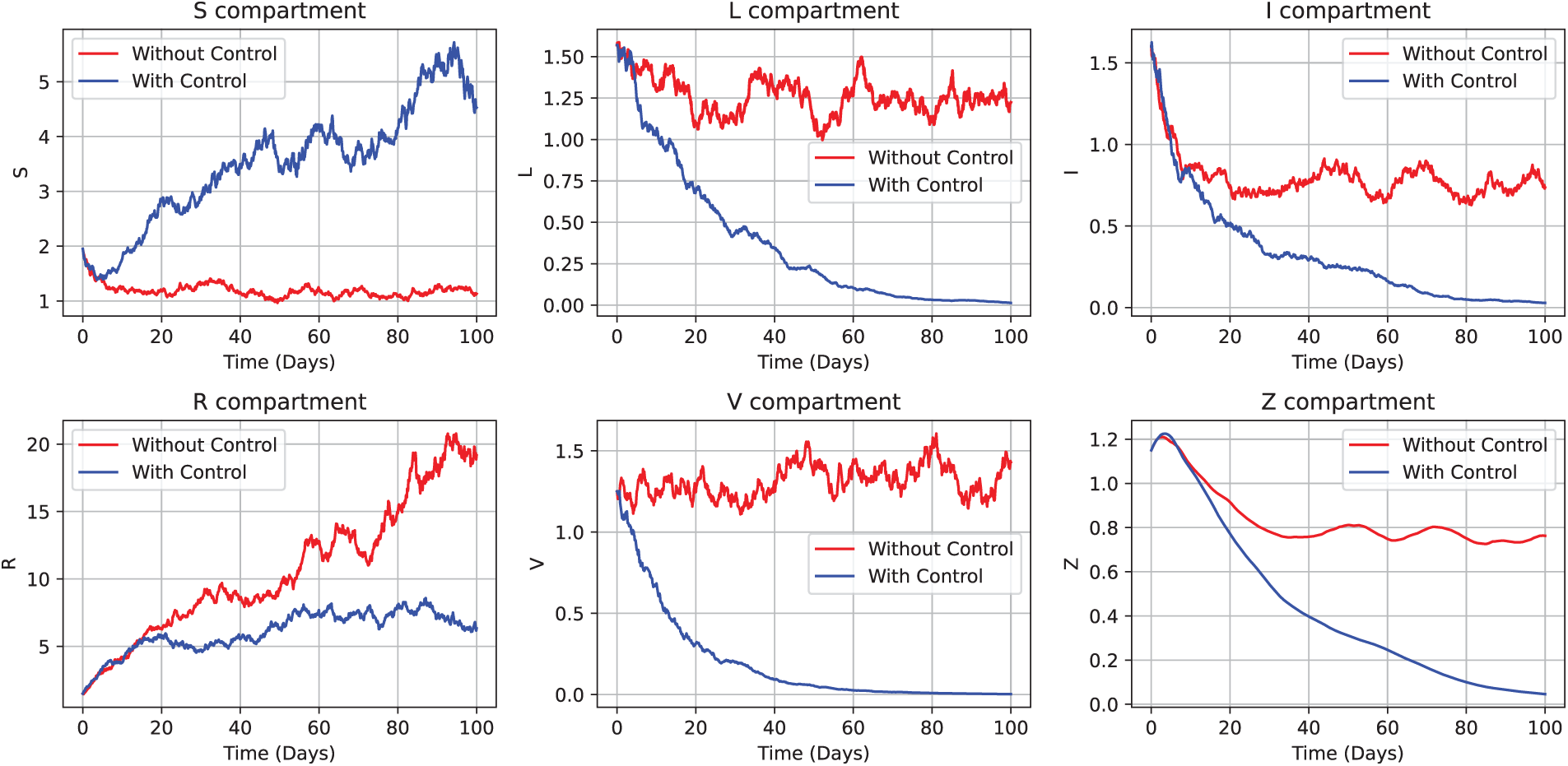
Figure 16: Illustration of the age-structured stochastic CHIKV model (52) dynamics incorporating control variables
Meanwhile, this analysis incorporates time-dependent control functions and Hamiltonian analysis to derive near-optimal intervention strategies. Each compartment, including susceptible
The control strategies
This framework facilitates a rigorous evaluation of age-specific intervention impacts in the presence of stochastic fluctuations, including behavioral variability and environmental noise, modeled through Poisson random measures. The effectiveness of these control strategies is demonstrated in Fig. 17, where the susceptible subpopulation,
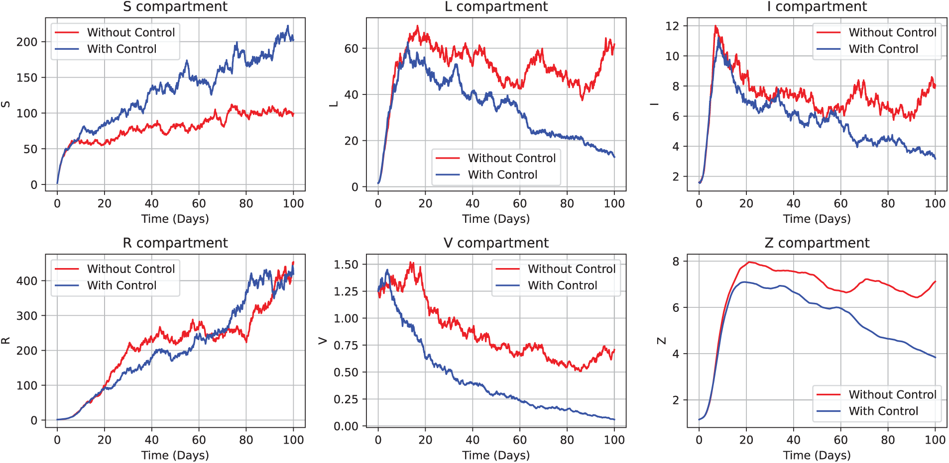
Figure 17: Depiction of the optimal control strategies
Moreover, near-optimal control theory, particularly when formulated through Hamiltonian structures and adjoint equations, has proven robust in epidemiological modeling where exact optimal controls are either infeasible or prohibitively costly. By leveraging the sufficiency and necessary optimality conditions (as derived in Theorem 9), the framework ensures that the proposed control strategy performs closely to an ideal optimal scenario without incurring prohibitive computational or logistical costs. This aligns with the broader stochastic control literature in mathematical epidemiology, which emphasizes trade-offs between intervention costs and epidemic mitigation [70]. Fig. 18 illustrates the decline in the infected class and the stabilization of virus/pathogen compartments under this control regime. These outcomes emphasize the importance of both the timing and intensity of interventions in managing outbreaks, especially under conditions of uncertainty.
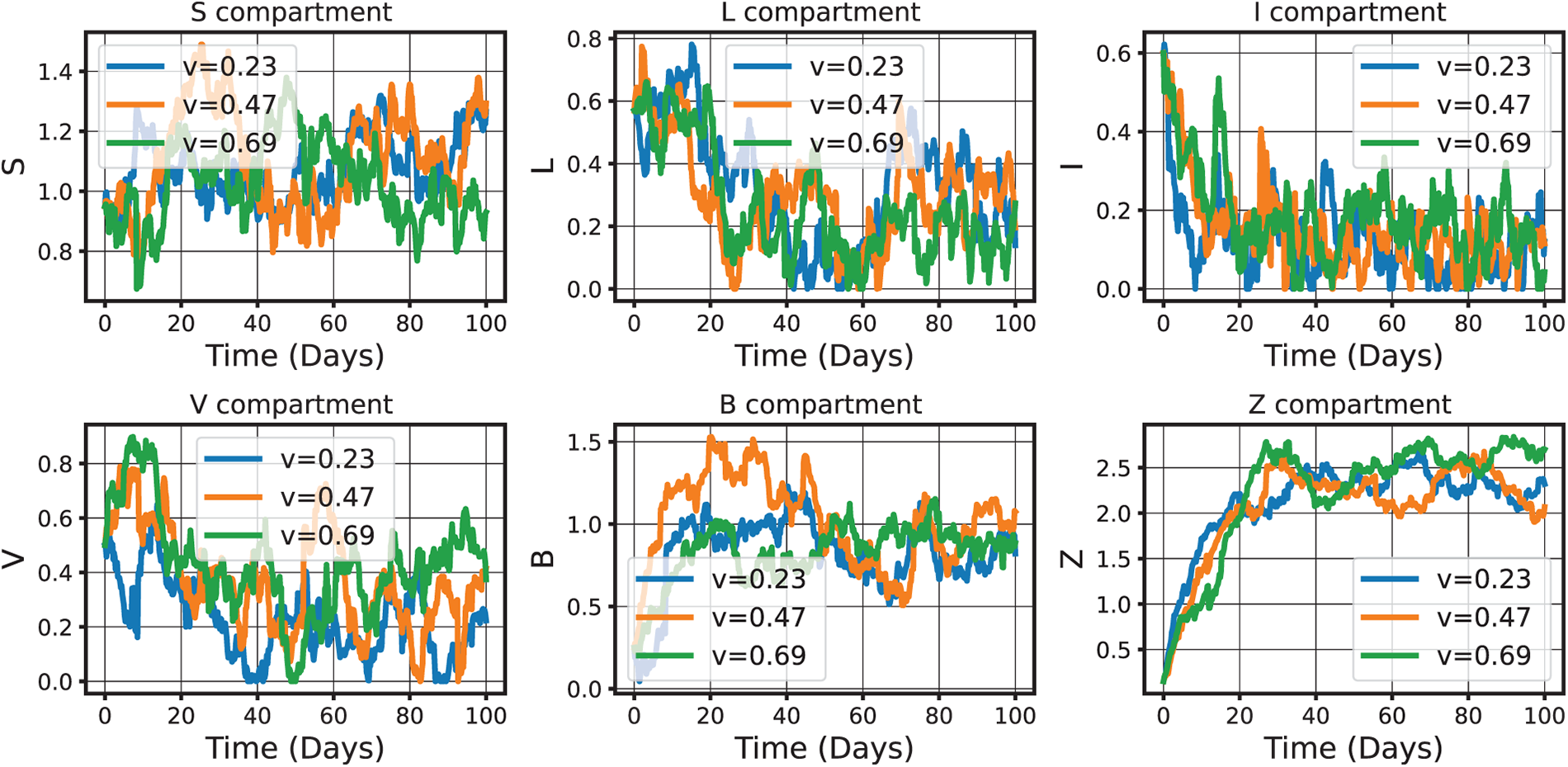
Figure 18: Graphical illustration decline in the infected class and stabilization of virus/pathogen compartments under an age-structured stochastic CHIKV model (52) with near-optimal control. The model incorporates age-specific compartments and stochastic perturbations, such as Lévy noise, to capture abrupt real-world events. Intervention strategies, including age-targeted vaccination and vector control, aim to minimize a cost functional balancing epidemiological outcomes with control efforts describing the necessary criteria of Theorem 9. This approach provides a rigorous and empirically grounded methodology for designing and analyzing intervention policies in the presence of demographic diversity and random fluctuations
Together, these strands of literature validate the formulation of an age-structured stochastic CHIKV model embedded with near-optimal control. This approach provides a mathematically rigorous and empirically grounded framework for designing and analyzing intervention policies in the face of demographic diversity and random perturbations.
The figure illustrates an age-structured model for CHIKV, where the human population is divided into three epidemiological states—susceptible, latent, and infectious—across each age group
Transitions between compartments are governed not only by deterministic epidemiological rates (e.g., transmission, immunization, recovery) but also by stochastic perturbations, which are modeled through a Poisson random measure superimposed with L’evy noise. This framework enables the simulation of abrupt random events, such as climate anomalies, vector density surges, or behavioral changes—phenomena increasingly observed in real epidemics, as highlighted in studies like that of Applebaum [72].
Superimposed on this structure are control arrows representing intervention strategies, denoted by the control process defined in Theorem 9, which satisfies
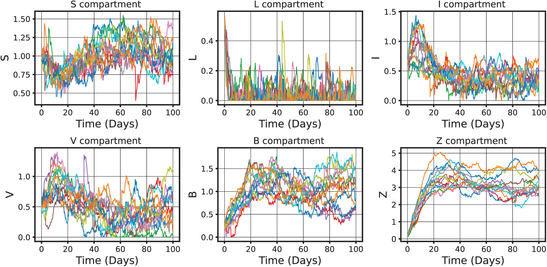
Figure 19: Highlights for the interconnectedness of age-specific compartments and the multi-objective nature of CHIKV epidemic model (52) control under uncertainty. Governed by a Hamiltonian framework, the near-optimal control conditions ensure robustness against stochastic perturbations. The model integrates age structure, stochastic dynamics, and optimal control theory, providing a reliable and biologically informed basis for policy design supported by the argument of Theorem 9, such as
CHIKV, an arthropod-transmitted alphavirus of the Togaviridae family, remains one of the most significant arthropod-borne viral infections in humans. This study presents a non-autonomous SDE model that incorporates age-structured dynamics and time-dependent prevalence variations to examine the impact of screening and therapeutic strategies on CHIKV spread. By modeling stochastic disruptions through Poisson random measures, the methodology captures sudden and unexpected changes influencing CHIKV transmission. For the Lévy-based model, we derive global positive solutions, ensuring the system’s biological feasibility.
The main contributions have been presented as:
• Developed an age-structured stochastic model that integrates demographic, immunization, and therapeutic interventions to more accurately estimate the basic reproduction number (
• Applied MCMC calibration to fit model predictions to monthly CHIKV incidence data (Florida, USA, 2005–2017), estimating undetermined parameters and initial conditions reliably.
• Provided sensitivity assessments across age groups using 95% confidence intervals, prediction intervals, and training-testing validation, offering practical insights into which populations are most at risk.
• Derived near-optimal control strategies using linear constraints and Ekeland’s variational principle, enabling precise evaluation of interventions.
• The model can guide public health interventions by identifying age groups with higher CHIKV incidence and evaluating the impact of vaccination and treatment strategies.
• Computed threshold parameter
• Predictions show that individuals over 66 years old have the highest incidence, while those under 16 are least affected, allowing targeted interventions.
Furthermore, future directions include extending the model to multi-variable systems with co-infections and environmental factors, using advanced methods such as deep learning or Kalman filters to improve predictions and validation across regions. The study is limited by assumptions of homogeneous mixing, ignored spatial or vector heterogeneity, and higher computational costs. Despite these, the framework offers valuable insights for CHIKV control and epidemic modeling.
Acknowledgement: The authors would like to thank the Ongoing Research Funding program (ORF-2025-1404), King Saud University, Riyadh, Saudi Arabia.
Funding Statement: Ongoing Research Funding program (ORF-2025-1404), King Saud University, Riyadh, Saudi Arabia.
Author Contributions: The authors confirm contribution to the paper as follows: study conception and design: Maysaa Al-Qurashi, Ayesha Siddiqa; data collection: Shazia Karim, Yu-Ming Chu; analysis, project administration and interpretation of results: Saima Rashid; draft manuscript preparation: Ayesha Siddiqa, Yu-Ming Chu. All authors reviewed the results and approved the final version of the manuscript.
Availability of Data and Materials: Data sharing not applicable to this article as no datasets were generated or analyzed during the current study.
Ethics Approval: Not applicable.
Conflicts of Interest: The authors declare no conflicts of interest to report regarding the present study.
References
1. World Health Organization. Global chikungunya report 2021. Comput Electr Eng. 2021;92:107129. [Google Scholar]
2. Fritsch H, Giovanetti M, Xavier J, Adelino TER, Fonseca V, de Jesus JG, et al. Retrospective genomic surveillance of chikungunya transmission in Minas Gerais State, Southeast Brazil. Microbiol Spectr. 2022;10(5):e0128522. doi:10.1128/spectrum.01285-22. [Google Scholar] [PubMed] [CrossRef]
3. Cerqueira-Silva T, Pescarini JM, Cardim LL, Leyrat C, Whitaker H, Antunes de Brito CA, et al. Risk of death following chikungunya virus disease in the 100 million Brazilian cohort, 2015–2018: a matched cohort study and self-controlled case series. Lancet Infect Dis. 2024;24:504–13. doi:10.1016/S1473-3099(23)00567-8. [Google Scholar] [CrossRef]
4. Khongwichit S, Chansaenroj J, Chirathaworn C, Poovorawan Y. Chikungunya virus infection: molecular biology, clinical characteristics, and epidemiology in Asian countries. J Biomed Sci. 2021;28(1):84. doi:10.1186/s12929-021-00778-8. [Google Scholar] [PubMed] [CrossRef]
5. Traverse EM, Millsapps EM, Underwood EC, Hopkins HK, Young M, Barr KL. Chikungunya immunopathology as it presents in different organ systems. Viruses. 2022;14(8):1786. doi:10.3390/v14081786. [Google Scholar] [PubMed] [CrossRef]
6. Costa D, Gouveia P, Silva GEB, Neves P, Vajgel G, Cavalcante M, et al. The relationship between chikungunya virus and the kidneys: a scoping review. Rev Med Virol. 2023;33(1):e2357. doi:10.1002/rmv.2357. [Google Scholar] [PubMed] [CrossRef]
7. Brandler S, Ruffié C, Combredet C, Brault J-B, Najburg V, Prevost M-C, et al. A recombinant measles vaccine expressing chikungunya virus-like particles is strongly immunogenic and protects mice from lethal challenge with chikungunya virus. Vaccine. 2013;31(36):3718–25. doi:10.1016/j.vaccine.2013.05.086. [Google Scholar] [PubMed] [CrossRef]
8. Chattopadhyay S, Roy A, Banerjee A, Goswami R, Basu A, Jana AM. Development and characterization of monoclonal antibody against non-structural protein-2 of chikungunya virus and its application. J Virol Methods. 2014;199:86–94. doi:10.1016/j.jviromet.2014.01.008. [Google Scholar] [PubMed] [CrossRef]
9. Mavale M, Parashar D, Sudeep A, Yadav PD, Gokhale MD, Mourya DT. Venereal transmission of chikungunya virus by Aedes aegypti mosquitoes (Diptera: culicidae). Am J Trop Med Hyg. 2010;83(6):1242–4. doi:10.4269/ajtmh.2010.09-0577. [Google Scholar] [PubMed] [CrossRef]
10. Goh LY, Tan HC, Lim XF, Ho BC, Sam IC, Chan YF, et al. Neutralizing monoclonal antibodies to the E2 protein of chikungunya virus protects against disease in a mouse model. Clin Immunol. 2013;149(3):487–97. doi:10.1016/j.clim.2013.10.004. [Google Scholar] [PubMed] [CrossRef]
11. Sourisseau M, Schilte C, Casartelli N, Trouillet C, Guivel-Benhassine F, Rudnicka D, et al. Characterization of reemerging chikungunya virus. PLoS Pathog. 2007;3(6):e89. doi:10.1371/journal.ppat.0030089. [Google Scholar] [PubMed] [CrossRef]
12. Gérardin P, Barau G, Michault A, Bintner M, Randrianaivo H, Choker G, et al. Multidisciplinary prospective study of mother-to-child chikungunya virus infections on the island of La Réunion. PLoS Med. 2008;5:e60. [Google Scholar]
13. Rezza G, Nicoletti L, Angelini R, Romi R, Finarelli AC, Panning M, et al. Infection with chikungunya virus in Italy: an outbreak in a temperate region. Lancet. 2007;370(9602):1840–6. doi:10.1016/s0140-6736(07)61779-6. [Google Scholar] [PubMed] [CrossRef]
14. Reiter P, Fontenille D, Paupy C. Aedes albopictus as an epidemic vector of chikungunya virus: another emerging problem? Lancet Infect Dis. 2006;6(8):463–4. doi:10.1016/s1473-3099(06)70531-x. [Google Scholar] [PubMed] [CrossRef]
15. Servant MJ, Tenoever B, Lin R. Overlapping and distinct mechanisms regulating IRF-3 and IRF-7 function. J Interferon Cytokine Res. 2002;22(1):49–58. doi:10.1089/107999002753452656. [Google Scholar] [PubMed] [CrossRef]
16. Brito CA, Teixeira MG. Increased number of deaths during a chikungunya epidemic in Pernambuco, Brazil. Mem Inst Oswaldo Cruz. 2017;112(9):650–1. doi:10.1590/0074-02760170124. [Google Scholar] [PubMed] [CrossRef]
17. Blasius AL, Giurisato E, Cella M, Schreiber RD, Shaw AS, Colonna M. Bone marrow stromal cell antigen 2 is a specific marker of type I IFN-producing cells in the naive mouse, but a promiscuous cell surface antigen following IFN stimulation. J Immunol. 2006;177(5):3260–5. doi:10.4049/jimmunol.177.5.3260. [Google Scholar] [PubMed] [CrossRef]
18. Rashid S, Jarad F. Novel investigation of stochastic fractional differential equations measles model via the white noise and global derivative operator depending on mittag-leffler kernel. Comput Model Eng Sci. 2024;139(3):2289–327. doi:10.32604/cmes.2023.028773. [Google Scholar] [CrossRef]
19. Arif MS, Abodayeh K, Nawaz Y. Construction of a computational scheme for the fuzzy HIV/AIDS epidemic model with a nonlinear saturated incidence rate. Comput Model Eng Sci. 2024;138(2):1405–25. doi:10.32604/cmes.2023.028946. [Google Scholar] [CrossRef]
20. Jajarmi A, Baleanu D, Rezapour S, Mohammadi H. A new fractional analysis on the interaction of HIV with CD4+ T-cells. Chaos Soliton Fract. 2018;115(4):1–10. doi:10.1016/j.chaos.2018.06.009. [Google Scholar] [CrossRef]
21. Bellan SE. The importance of age dependent mortality and the extrinsic incubation period in models of mosquito-borne disease transmission and control. PLoS One. 2010;5(4):e10165. [Google Scholar] [PubMed]
22. Olayiwola MO, Oluwafemi EA. Modeling tuberculosis dynamics with awareness and vaccination using laplace-adomian and fractional calculus. Iran J Sci. 2025;1(1):78. doi:10.1007/s40995-025-01830-0. [Google Scholar] [CrossRef]
23. Olayiwola MO, Tijani KR, Ogunniran MO, Yunus AO, Oluwafemi EA, Abanikanda MO, et al. Modeling the booster vaccine effect on new COVID-19 variant management employs the Atangana-Baleanu-Caputo fractional derivative operator together with the Laplace-Adomian decomposition method. Vacunas. 2025;26(3):500458. doi:10.1016/j.vacun.2025.500458. [Google Scholar] [CrossRef]
24. Mohamed Ali H, Mahdy AM, El-Mesady A. Investigation of stability criteria and optimal control measures for a fractional-order model of human papillomavirus infection and cervical cancer. Int J Biomathematics. 2025;18:1–15. doi:10.1142/s1793524525500639. [Google Scholar] [CrossRef]
25. El-Mesady A, Al-Shami TM, Ali HM. Optimal control efforts to reduce the transmission of HPV in a fractional-order mathematical model. Bound Value Probl. 2025;42(1):1–18. doi:10.1186/s13661-024-01991-8. [Google Scholar] [CrossRef]
26. Buonomo B. Analysis of a malaria model with mosquito host choice and bed-net control. Int J Biomathematics. 2015;8(1550):077. doi:10.1142/s1793524515500771. [Google Scholar] [CrossRef]
27. Chitnis N, Smith T, Steketee R. A mathematical model for the dynamics of malaria in mosquitoes feeding on a heterogeneous host population. J Biol Dyn. 2008;2(3):259–85. doi:10.1080/17513750701769857. [Google Scholar] [PubMed] [CrossRef]
28. Zhang L, Zhou Q, Yang J. Necessary condition for optimal control of doubly stochastic systems. Math Control Relat Fields. 2020;10(2):379–403. doi:10.3934/mcrf.2020002. [Google Scholar] [CrossRef]
29. Huang J, Li X, Wang G. Near-optimal control problems for linear forward-backward stochastic systems. Automatica. 2010;46(2):397–404. doi:10.1016/j.automatica.2009.11.016. [Google Scholar] [CrossRef]
30. Yong J, Zhou X. Stochastic control: hamilton systems and HJB equations. New York, NY, USA: Springer; 1999. [Google Scholar]
31. Ji C. Dynamics of a multigroup SIR epidemic model with stochastic perturbation. Automatica. 2012;48(8):1859–67. doi:10.1016/j.automatica.2011.09.044. [Google Scholar] [CrossRef]
32. Yang Q. The ergodicity and extinction of stochastically perturbed SIR and SEIR epidemic models with saturated incidence. J Math Anal Appl. 2012;386(2):722–38. doi:10.1016/j.jmaa.2011.11.072. [Google Scholar] [CrossRef]
33. Dereich S, Heidenreich F, Scheutzow M. A multilevel Monte Carlo algorithm for Lévy-driven stochastic differential equations. Stochastic Process Appl. 2011;121(12):2597–17. doi:10.1016/j.spa.2011.03.015. [Google Scholar] [CrossRef]
34. Rubenthaler S. Numerical simulation of the solution of a stochastic differential equation driven by a Lévy process. Stochastic Process Appl. 2003;103(2):313–32. doi:10.1016/s0304-4149(02)00191-6. [Google Scholar] [CrossRef]
35. Zhou Y, Yuan S, Zhao D. Threshold behavior of a stochastic SIS model with Lévy jumps. Appl Math Comput. 2016;275:255–67. [Google Scholar]
36. Liu M, Bai C. Optimal harvesting of a stochastic mutualism model with Lévy jumps. Appl Math Comput. 2016;276(247):301–9. doi:10.1016/j.amc.2015.11.089. [Google Scholar] [CrossRef]
37. Shu H, Jin HY, Wang XS, Wu J. Viral infection dynamics with immune chemokines and CTL mobility modulated by the infected cell density. J Math Biol. 2024;88(4):43. [Google Scholar] [PubMed]
38. Dubey P, Dubey US, Dubey B. Modeling the dynamics of viral-host interaction during treatment of productively infected cells and free virus involving total immune response. Nonlinear Anal Model Control. 2021;26(4):678–701. doi:10.15388/namc.2021.26.21434. [Google Scholar] [CrossRef]
39. Handel A, Antia R. A simple mathematical model helps to explain the immunodominance of CD8 T cells in influenza A virus infections. J Virol. 2008;82(16):7768–72. doi:10.1128/jvi.00653-08. [Google Scholar] [PubMed] [CrossRef]
40. Cui T, Liu P, Din A, Khan A. Impact of Lévy noise on a stochastic Norovirus epidemic model with information intervention. Math Methods Appl Sci. 2023;46(6):4715–30. doi:10.1002/mma.9655. [Google Scholar] [CrossRef]
41. Gikhman II, Skorokhod AV. Stochastic differential equations. Berlin/Heidelberg, Germany: Springer; 2007. [Google Scholar]
42. El Fatini M, Sekkak I. Lévy noise impact on a stochastic delayed epidemic model with Crowley-Martin incidence and crowding effect. Physica A. 2020;541(2):123315. doi:10.1016/j.physa.2019.123315. [Google Scholar] [CrossRef]
43. Din A, Li Y. Lévy noise impact on a stochastic hepatitis B epidemic model under real statistical data and its fractal-fractional Atangana–Baleanu order model. Phys Scr. 2021;96(12):124008. doi:10.1088/1402-4896/ac1c1a. [Google Scholar] [CrossRef]
44. Zhang XB, Wang XD, Huo HF. Extinction and stationary distribution of a stochastic SIRS epidemic model with standard incidence rate and partial immunity. Physica A. 2019;531(3):121548. doi:10.1016/j.physa.2019.121548. [Google Scholar] [CrossRef]
45. Song Y, Liu P, Din A. A novel stochastic model for human Norovirus dynamics: vaccination impact with Lévy noise. Fractal Fract. 2024;8(6):349. [Google Scholar]
46. Hafayed M, Abbas S. On near-optimal mean-field stochastic singular controls: necessary and sufficient premises for near-optimality. J Optim Theory Appl. 2014;160(3):778–808. doi:10.1007/s10957-013-0361-1. [Google Scholar] [CrossRef]
47. Liu Z, Guo S, Tan R, Liu M. Modeling and analysis of a non-autonomous single-species model with impulsive and random perturbations. Appl Math Model. 2016;40(9–10):5510–31. doi:10.1016/j.apm.2016.01.008. [Google Scholar] [CrossRef]
48. Kuang D, Li J, Gao D, Luo D. Stochastic near-optimal control for a system with Markovian switching and Lévy noise. Chaos Soliton Fract. 2024;178:114360. doi:10.1016/j.chaos.2023.114360. [Google Scholar] [CrossRef]
49. Donnelly C. Sufficient stochastic maximum principle in a regime-switching diffusion model. Appl Math Optim. 2011;64(2):155–69. doi:10.1007/s00245-010-9130-9. [Google Scholar] [CrossRef]
50. Peng S. A general stochastic maximum principle for optimal control problems. SIAM J Control Optim. 1990;28(4):966–79. doi:10.1137/0328054. [Google Scholar] [CrossRef]
51. Li M, Wu Z. Necessary and sufficient assertions of near-optimality in a regime-switching diffusion model. Optim Control Appl Methods. 2020;41(3):793–807. doi:10.1002/oca.2571. [Google Scholar] [CrossRef]
52. Mao X. Stochastic differential equations and applications. Amsterdam, The Netherland: Elsevier; 2007. [Google Scholar]
53. Ekeland I. On the variational principle. J Math Anal Appl. 1974;47(2):324–53. [Google Scholar]
54. Zhu Y, Wang L, Qiu Z. Dynamics of a stochastic cholera epidemic model with Lévy process. Physica A. 2022;595(1):127069. doi:10.1016/j.physa.2022.127069. [Google Scholar] [CrossRef]
55. Ain QT, Din A, Qiang X, Kou Z. Dynamics for a nonlinear stochastic cholera epidemic model under Lévy noise. Fractal Fract. 2024;8(5):293. doi:10.3390/fractalfract8050293. [Google Scholar] [CrossRef]
56. Mao X, Wei F, Wiriyakraikul T. Positivity preserving truncated Euler–Maruyama method for stochastic Lotka-Volterra competition model. J Comput Appl Math. 2021;394(3):113566. doi:10.1016/j.cam.2021.113566. [Google Scholar] [CrossRef]
57. Data-Center of USA Public Health Science. Data director [Internet]. 2023 [cited 2025 Jul 16]. Available from: https://www.phsciencedata.usa/Share/en/index.jsp. [Google Scholar]
58. Florida Department of Economic and Demographic Research, U.S. Census Bureau. Population data for florida, 2005–2019 [Internet]. 2023 [cited 2025 Jul 16]. Available from: http://edr.state.fl.us/Content/population-demographics/data/index.cfm. [Google Scholar]
59. Byers NM, Fleshman AC, Perera R, Molins CR. Metabolomic insights into human arboviral infections: dengue, Chikungunya, and Zika viruses. Viruses. 2019;11(3):225. doi:10.3390/v11030225. [Google Scholar] [PubMed] [CrossRef]
60. de Lima STS, de Souza WM, Cavalcante JW, Candido DDS, Fumagalli MJ, Carrera J-P, et al. Fatal outcome of Chikungunya virus infection in Brazil. Clin Infect Dis. 2021;73:2436–43. [Google Scholar]
61. Reisinger EC, Tschismarov R, Beubler E, Wiedermann U, Firbas C, Loebermann M, et al. Immunogenicity, safety, and tolerability of the measles-vectored Chikungunya virus vaccine MV-CHIK: a double-blind, randomised, placebo-controlled and active-controlled phase 2 trial. Lancet. 2018;392(10165):2718–27. doi:10.1016/s0140-6736(18)32488-7. [Google Scholar] [PubMed] [CrossRef]
62. Schilte C, Staikovsky F, Couderc T, Madec Y, Carpentier F, Roux K, et al. Correction: chikungunya virus-associated long-term arthralgia: a 36-month prospective longitudinal study. PLoS Negl Trop Dis. 2013;7(3):e2137. doi:10.1371/journal.pntd.0002137. [Google Scholar] [PubMed] [CrossRef]
63. Cazelles B, Chavez M, De Magny GC, Guegan J, Hales S. Time-dependent spectral analysis of epidemiological time-series with wavelets. J R Soc Interface. 2007;4(15):625–36. doi:10.1098/rsif.2007.0212. [Google Scholar] [PubMed] [CrossRef]
64. Centers for Disease Control and Prevention (CDC). Population census and population estimates [Internet]. 2023 [cited 2025 Jul 16]. Available from: https://www.cdc.gov/nchs/hus/sources-definitions/census-population.htm. [Google Scholar]
65. Haario H, Laine M, Mira A, Saksman E. DRAM: efficient adaptive MCMC. Stat Comput. 2006;16(4):339–54. doi:10.1007/s11222-006-9438-0. [Google Scholar] [CrossRef]
66. Cressie NAC. Statistics for spatial data. Revised ed. New York, NY, USA: Wiley; 1993. [Google Scholar]
67. Wikipedia. One in ten rule [Internet]. 2022 [cited 2025 Mar 26]. Available from: https://en.wikipedia.org/wiki/One_in_ten_rule. [Google Scholar]
68. McKay MD, Beckman RJ, Conover WJ. A comparison of three methods for selecting values of input variables in the analysis of output from a computer code. Technometrics. 1979;21(2):239–45. doi:10.1080/00401706.1979.10489755. [Google Scholar] [CrossRef]
69. Huang M, Caines PE. Pontryagin’s maximum principle for mean field stochastic control problems. SIAM J Control Optim. 2009;48(8):5145–75. [Google Scholar]
70. Esteva L, Vargas C. Analysis of a model for the transmission dynamics of the dengue virus in a human population. Math Biosci. 1998;149(1):41–61. doi:10.1016/S0025-5564(98)00006-6. [Google Scholar] [CrossRef]
71. Agusto FB, Mbohwa C, Lokossou T. Modeling and analysis of age-structured population for the control of vector-borne diseases. Math Biosci Eng. 2016;13(2):263–81. doi:10.3934/mbe.2016.13.263. [Google Scholar] [CrossRef]
72. Applebaum D. Lévy processes and stochastic calculus. 2nd ed. Cambridge, UK: Cambridge University Press; 2009. [Google Scholar]
73. Fleming WH, Rishel RW. Deterministic and stochastic optimal control. 1st ed. New York, NY, USA: Springer-Verlag; 1975. [Google Scholar]
74. Buckwar E, Riedler M. Adaptive control for stochastic epidemic models. Math Biosci Eng. 2011;8(4):935–50. doi:10.3934/mbe.2011.8.935. [Google Scholar] [CrossRef]
Cite This Article
 Copyright © 2025 The Author(s). Published by Tech Science Press.
This work is licensed under a Creative Commons Attribution 4.0 International License , which permits unrestricted use, distribution, and reproduction in any medium, provided the original work is properly cited.
 Downloads
 Citation Tools