A Computational Modeling Approach for Joint Calibration of Low-Deviation Surgical Instruments

1  Introduction

With the advancement of society, increasing attention to individual health has been accompanied by growing investments in healthcare technologies [1,2]. Engineering and technical professionals increasingly offer technical support to physicians based on specific clinical needs. The close cooperation between technology experts and medical professionals has significantly accelerated the development of medical technology, leading to the emergence of numerous innovative techniques. Among these innovations, image-guided surgical techniques [3–6], a cutting-edge minimally invasive treatment, have become widely adopted.

CT scans, fluoroscopy, magnetic resonance imaging (MRI), or ultrasound images are usually used to guide needle insertion in minimally invasive medical procedures. The use of CT has limitations, primarily due to the high doses of ionizing radiation patients are exposed to during the procedure [7]. Instruments made of non-magnetic and dielectric materials are restricted to permeabilization procedures [8]. Ultrasound is considered a safe and readily available imaging modality for observing needles and targets during surgery [9–11].

Calibration of surgical instruments is essential for surgical navigation before surgery [12–14]. The accuracy of instruments calibration determines the overall precision of surgical navigation, playing a critical role in the effectiveness and safety of surgery. Thus, the positioning and calibration of the probe needle in the surgical navigation systems remains a research focus. Traditional hand-eye calibration methods are challenging to implement in the confined spaces of the body. To address this challenge, researchers have proposed an autonomous instrument calibration method using a monocular camera [15]. This method utilizes visual feedback to track the instrument’s motion trajectory, followed by a two-stage parameter estimation process to achieve autonomous calibration. This approach overcomes the limitations of hand-eye observation, enhancing the safety of minimally invasive surgery. Some researchers have shifted their focus to surgical instruments, such as robotic arms, applying image-guided techniques to track their paths [16,17]. An economical, high-precision optical tracking system has been introduced by researchers. Within this system, Bumblebee2 stereo cameras are utilized to capture images of objects marked with distinctive identifiers. The central pixel coordinates of these markers are extracted, and specialized image processing techniques are applied to reconstruct the coordinates of the surgical instrument’s tip, facilitating tracking. This approach significantly enhances the system’s resilience to interference.

In recent years, the precision of surgical navigation systems has increasingly relied on accurate localization of the needle tip and robust calibration of ultrasound probes. However, most existing methods approach these two processes independently, leading to cumulative spatial errors during interventional procedures. For instance, Beigi et al. [18] developed techniques to enhance needle visibility and localization in ultrasound images, yet their method focuses solely on image-based improvements without addressing hardware alignment or spatial registration. Recent advancements have also proposed calibration schemes for ultrasound probes using either phantoms or robotic assistance. Wang et al. [19] introduced a dual-arm surgical navigation platform with independent ultrasound probe calibration via fiducial phantoms, achieving reasonable precision but at the cost of system complexity and multi-step workflows. Meanwhile, Seitel et al. [20] employed miniaturized electromagnetic tracking to guide needle insertions in real time, demonstrating accuracy improvements but still requiring separate probe-needle calibration steps. More recently, Che et al. [21] utilized deep learning to improve needle tip detection in ultrasound-based navigation, but their framework assumes pre-calibrated devices and does not consider joint optimization. These studies collectively reveal a significant research gap: there remains a lack of integrated calibration models that simultaneously account for both needle tips and ultrasound probe alignment within a unified coordinate system. This fragmentation results in accumulated spatial errors and hinders real-time surgical adaptability.

Despite progress in individual domains of needle tracking and ultrasound probe calibration, a major limitation remains: the absence of a unified, model-driven calibration framework that directly relates the physical space of the surgical instrument to the imaging plane of the ultrasound probe in a mathematically consistent and spatially coherent manner. Existing techniques typically decouple the two processes: first localizing the needle tip through geometric constraints, then calibrating the probe separately using phantoms or empirical image mappings. This two-stage pipeline introduces cumulative transformation errors, increases system complexity, and often requires manual intervention or fiducial markers, which are undesirable in real-time, minimally invasive procedures.

In contrast, our work introduces a joint calibration model that integrates both the needle tip localization and the ultrasound probe-to-image plane calibration within a shared coordinate system, supported by explicit coordinate transformation and optimization models. By leveraging the constrained spherical motion of the instrument during rotation, we formulate a gradient-descent-based solution to estimate the true spatial position of the needle tip. This result is then used as a geometric anchor in an N-line ultrasound calibration model, allowing the system to compute the spatial transformation between the ultrasound image plane and the physical coordinate frame without relying on external phantoms. Our approach thus not only reduces system complexity and accumulated error but also demonstrates submillimeter localization accuracy (0.1644 mm) and low pixel deviation in image alignment (1.2373 mm), validated across 253-frame sequences. These contributions position our method as a practical and precise calibration strategy for real-time ultrasound-guided surgical navigation, especially in scenarios requiring portability, reduced radiation exposure, and high spatial fidelity. It fills a critical gap in the literature by offering an end-to-end mathematical framework that bridges the calibration of hardware (needle and probe) with imaging output in a single optimization loop.

2  Method

Initially, capturing the tip of the surgical instrument is essential. After the initial capturing of the tip, the next step is to establish the optical positioning systems for both the surgical instrument and its tip. Using optical positioning, the three-dimensional spatial coordinates of three non-collinear feature points on the surgical instrument, along with the coordinates of the tip, are captured. Next, the spatial coordinates of the instrument’s tip point are determined relative to its own coordinate system. As the surgical instrument rotates around its tip, the three non-collinear points trace paths on a concentric spherical surface. Leveraging this spherical motion constraint, the spatial coordinates of the tip can be precisely calibrated within the coordinate system defined by the surgical instrument. This method ensures high accuracy in the calibration process, which is vital for the precision and reliability of surgical navigation systems.

2.1 Optimal Rotation Algorithm

The optimal rotation algorithm [22] is used to determine the rotation and translation matrix between coordinate systems, as shown in Fig. 1.

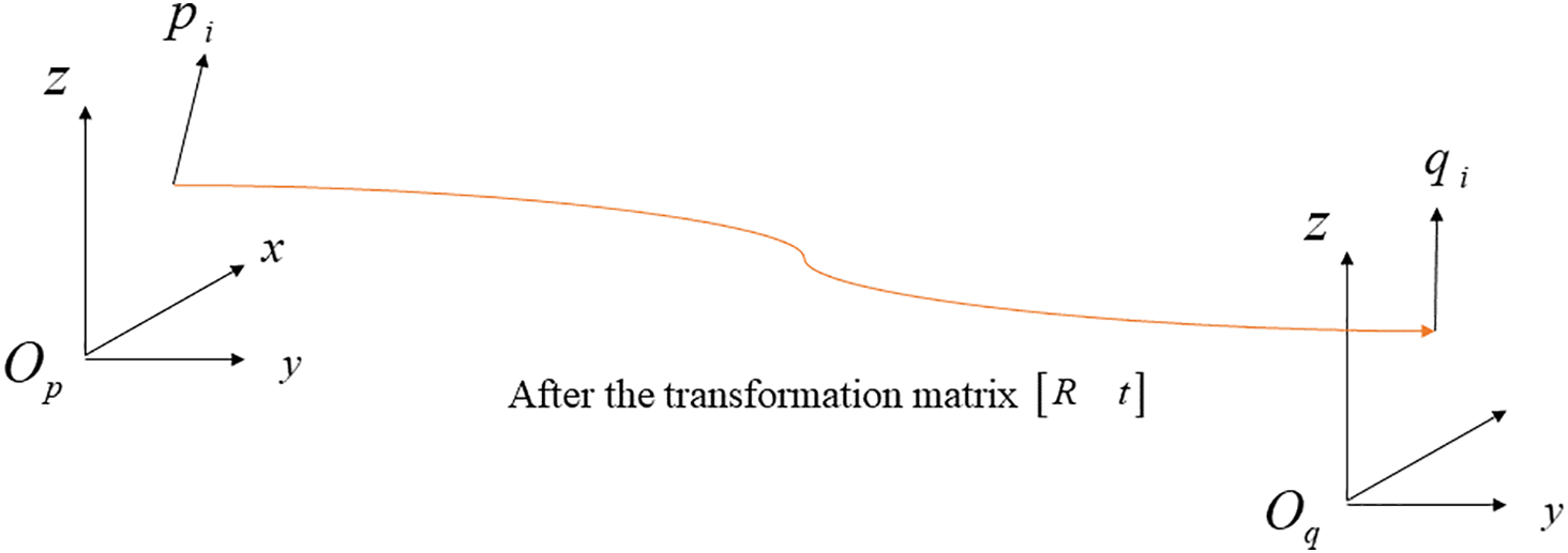
Figure 1: Schematic diagram of the optimal rotation algorithm

The optimization objective is shown in Eq. (1):

θ∗=arg⁡minθ(1N∑i=1N‖R⋅pi+t−qi‖22)(1)

where qi=[Xqi,Yqi,Zqi]T,i=1,2,…,N. Parameter R represents the rotation matrix where point pi is transformed to qi, and t represents the translation vector of point pi transformation to qi, θ denotes the solved quantity and θ=[R,t].

2.2 Calibration of Puncture Needle Tips

Tracking and positioning surgical instruments during surgery is a fundamental task in surgical navigation. The spatial coordinates of these instruments can be accurately determined by referencing non-collinear landmarks on their structure. Fig. 2 clearly demonstrates this calibration process, using four specific marking points on a surgical instrument as an example. Once the instrument’s movement stabilized, the tip of the surgical instrument is established as the center of a sphere, with the four landmarks positioned on its surface. This method provides a robust calibration technique, which is essential for the accuracy and effectiveness of surgical navigation systems.

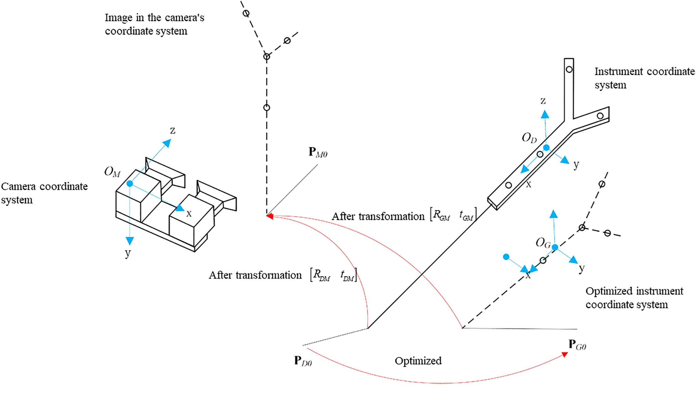
Figure 2: Needle tip calibration model

2.2.1 Problem Formulation

To calculate the coordinates of the tip point in the instrument coordinate system, a common method involves fixing the tip of the surgical instrument, rotating the instrument around this fixed point, using an optical tracking system to collect the positions of the surgical instrument’s marking points, and then calculating the transformation matrix [Tdm,tdm] of the instrument coordinate system [ODXDYDZD] to the camera coordinate system [OMXMYMZM].

The matrix form of the coordinate system in the instrument coordinate system is shown in the Eq. (2).

PD=[pD0,pD1,pD2,pD3,pD4](2)

where PD is a matrix of 3×5 dimensions, pD0 represents the coordinates of the tip in the coordinate system of the instrument, and pD1, pD2, pD3, pD4 represent the coordinates of the first, second, third, and fourth optical markers in the instrument’s coordinate system, respectively.

The matrix form of the coordinate system in the camera coordinate system is shown in the Eq. (3).

PM=[pM0,pM1,pM2,pM3,pM4](3)

where PM is a matrix of 3×5 dimensions, pM0 represents the coordinates of the needle tip in the camera coordinate system, and pM1, pM2, pM3, pM4 represent the coordinates of the first, second, third, and fourth optical markers in the camera coordinate system, respectively.

The transformation of coordinates from the instrument coordinate system to the camera coordinate system is an indirect process. First, the instrument coordinate system OGXGYGZG is optimized. Then, the optimized needle tip coordinates are converted to the camera coordinate system.

The matrix representation of the optimized instrument coordinate system is shown in Eq. (4).

PG=[pG0,pG1,pG2,pG3,pG4](4)

where PG is a matrix of 3×5 dimensions, pG0 represents the coordinates of the needle tip in the optimized instrument coordinate system, and pG1, pG2, pG3, pG4 represent the coordinates of the first, second, third, and fourth optical spheres in the optimized instrument coordinate system, respectively.

The transformation relationship between optimized instrument coordinate and camera coordinate is shown in the Eq. (5).

PM=[RGMtGM][PG11111](5)

where RGM denotes the rotation matrix that transforms points from the optimized instrument coordinate system to the camera coordinate system, and tGM represents the translation vector for this transformation.

Since PM is known, only two variables tGM and PG remains. The calibration process of calibration of the surgical instrument tip involves solving the Eq. (5), which can typically be done using two positioning images. However, the calculation of tGM and PG based on the experimental results obtained from the two images is inaccurate, so we collect T images for greater precision.

The calibration formula for the puncture tip is shown in Eq. (6).

pM0(k)=[RGM(k)tGM(k)][pG01],(k=1,2,3,…,T)(6)

where k denotes the k-th image captured within the camera coordinate system. The coordinates of the needle tip in this k-th image, relative to the camera coordinate system, are represented by pM0(k). Furthermore, RGM(k) signifies the rotation matrix used to transform points from the optimized instrument coordinate system to corresponding points in the k-th image within the camera coordinate system. Lastly, tGM(k) represents the translation vector required to map a point from the optimized instrument coordinate system to its position in the k-th camera image.

According to Eq. (6), the needle tip coordinates obtained from the T images are averaged to derive Eq. (7):

p0¯=1N∑k=1T(RGM(k)pG0+tGM(k))(7)

The Mean Square Error (MSE) of the tip position is shown in Eq. (8):

EMSE=1T∑k=1T‖RGM(k)pG0+tGM(k)−p0¯‖22(8)

The optimization problem is shown in Eq. (9).

θ0∗=arg⁡minθ0EMSE(9)

where θ0=pG0, RGM(k) and tGM(k) can be calculated by the Eq. (1), and θ0∗ represents the needle tip coordinates under the instrument coordinate system optimized by gradient descent, where the MSE of the tip position is the smallest.

2.2.2 Problem Solving

According to the gradient descent method [23,24], the solution to Eq. (9), as illustrated in Fig. 3, can be formulated as follows:

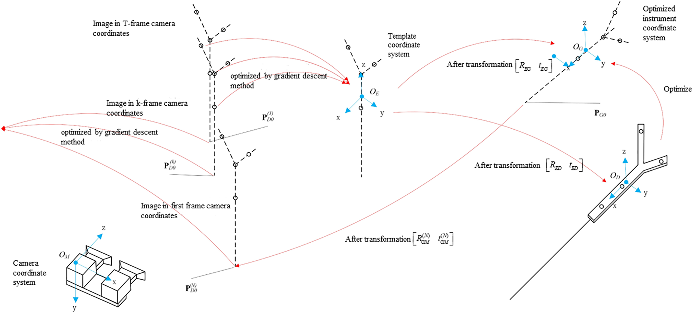
Figure 3: Calibration process of puncture needle tip

The template coordinate system is optimized based on the image of the T-group optical spheres captured in the camera coordinate system.

The coordinates of the optical sphere of the template coordinate system are transformed into the instrument coordinate system, and the rotation transformation matrix [REDtED] can be derived using the optimal rotation algorithm.

To account for inherent errors in the coordinate system transitions from the optimal rotation algorithm, the template coordinate system’s coordinates are converted to the optimized instrument coordinate system using a rotation transformation matrix [RGDtGD]. This process refines the coordinates of the optical sphere in the instrument coordinate system.

The gradient descent method is used to solve the objective function, yielding the coordinates of the needle tip in the optimized instrument coordinate system.

Initially, we optimized the template coordinate system. By rotating the needle tip around a fixed point, we captured T images, from which we extract the coordinates of T sets of four optically marked spheres. Using binocular vision calibration, we obtain the coordinates of the four optical marker spheres in the coordinate system of T camera: [pM1(k),pM2(k),pM3(k),pM4(k)](k=1,2,3,…,T). Utilizing the known design dimension of the puncture needle, denoted as [pD1,pD2,pD3,pD4], we calculate the coordinate of the four optical spheres in the instrument coordinate system. Furthermore, measurements allow us to estimate the coordinates of the needle tip, designated as pD0, in the instrument coordinate system.

The T groups of optical spheres’ coordinate can be optimized using gradient descent to establish a template coordinate system OEXEYEZE. The coordinates of the four optical spheres in the template coordinate system are represented as [pE1,pE2,pE3,pE4], as shown in Eq. (10).

[REM(k)tEM(k)][pE1pE2pE3pE41111]=[pM1(k)pM2(k)pM3(k)pM4(k)](10)

where [REM(k)tEM(k)] represents the rotation and translation matrix of the point transformation in the template coordinate system to the k-th image in the camera coordinate system.

The objective function of the template coordinate system is obtained as Eq. (11).

θe∗=argminθe‖E(θe)‖22(11)

where θe=[pE1pE2pE3pE4]T.

Taking the image coordinates from the first frame as the initial value: [pE1pE2pE3pE4]=[pM1(1)pM2(1)pM3(1)pM4(1)], we can get Eq. (12).

E(θe)=[E(θe)1E(θe)2⋅⋅⋅E(θe)T]E(θe)k=[REM(k)pE1+tEM(k)REM(k)pE2+tEM(k)REM(k)pE3+tEM(k)REM(k)pE4+tEM(k)](12)

where E(θe)k=1,2,3,…,T represents the value of the k-th image.

The Jacobi matrix is shown in Eq. (13). Where JEk=E1,E2,…,ET represents the Jacobi matrix of the k-th image.

JE=[JE1JE2⋅⋅⋅JEr]JEk=[δE(θe)kδE1δE(θe)kδE2δE(θe)kδE3δE(θe)kδE4](13)

The step size was set to α=0.01 based on empirical testing, which followed the standard gradient descent procedure and consistently achieved stable convergence without oscillation. Smaller values slowed convergence, while larger ones occasionally caused instability. Update the value according to Eq. (14).

θe∗=θe−αE(θe)TJE(14)

By iteratively updating θe∗ using the gradient descent method, the coordinates of the four optical spheres in the template coordinate system are determined, yielding [pE1pE2pE3pE4].

We can refine the tip’s coordinates within the instrument’s coordinate system. Initially, the coordinates of the four optical spheres are rotated and translated from the template coordinate system to align with the instrument coordinate system, as indicated in Eq. (15).

[REDtED][pE1pE2pE3pE41111]=[pD1pD2pD3pD4](15)

where [REDtED] can be obtained by the optimal rotation algorithm.

Due to the error e in the transformation between the coordinate systems as determined by the optimal rotation algorithm, the coordinate [pG1pG2pG3pG4] under the optimized instrument coordinate system can be calculated, as illustrated in Eq. (16).

[pG1pG2pG3pG4]=[REGtEG][pE1pE2pE3pE41111](16)

The coordinates in the template coordinate system are first rotated and translated to align with the optimized instrument coordinate system. Subsequently, these coordinates are transformed to the coordinate system of T groups of cameras, resulting in Eq. (17).

[RGM(k)tGM(k)][pG1pG2pG3pG41111]=[pM1(k)pM2(k)pM3(k)pM4(k)](17)

We convert the needle tip coordinates from the instrument coordinate system to the camera coordinate system, obtaining eight sets of coordinates in the camera’s frame of reference. Subsequently, the optimized tip coordinates were determined using the gradient descent method.

Solve the Eq. (9) using the objective optimization function illustrated in Eq. (18).

E(θ0)=[E(θ0)1E(θ0)2⋅⋅⋅E(θ0)r]E(θ0)i=RGM(k)θ0+tGM(k)−p0¯(18)

where E(θ0)k=1,2,…,r represents the value of the k-th graph.

The Jacobi matrix is illustrated in Eq. (19).

Jp=[Jp1Jp2⋅⋅⋅JpT](19)

where Jpk=p1,p2,…,pT.

Set step length α = 0.01 based on empirical testing to update the value according to Eq. (20).

θ0∗=θ0−αE(θ0)TJp(20)

The optimal tip coordinate θ0∗ is iteratively updating using the gradient descent method. This coordinate represents the calibrated tip in the instrument coordinate system.

By using the design coordinates of four optically marked spheres and a series of rotation translation matrices, the minimum value of the objective function is obtained, thus completing the optimization of the design coordinates.

2.3 Calibration of Ultrasound Probe

This study employs an optical tracking system [25,26] and proposes an innovative method for calibrating ultrasound probes based on the N-line method [27]. The method involves first calibrating the coordinates of endpoints of each line in the optical coordinate system using the puncture needle tip as a reference and then mapping the intersections of the N-line with the ultrasound image in the image coordinate system. Finally, the calibration equation is applied to determine the calibration results through substitution.

The principle involves obtaining a transformation matrix that aligns the spatial references of the ultrasound image with the corresponding probe, ensuring accurate spatial mapping across different coordinate systems. This concept is illustrated in the accompanying Fig. 4.

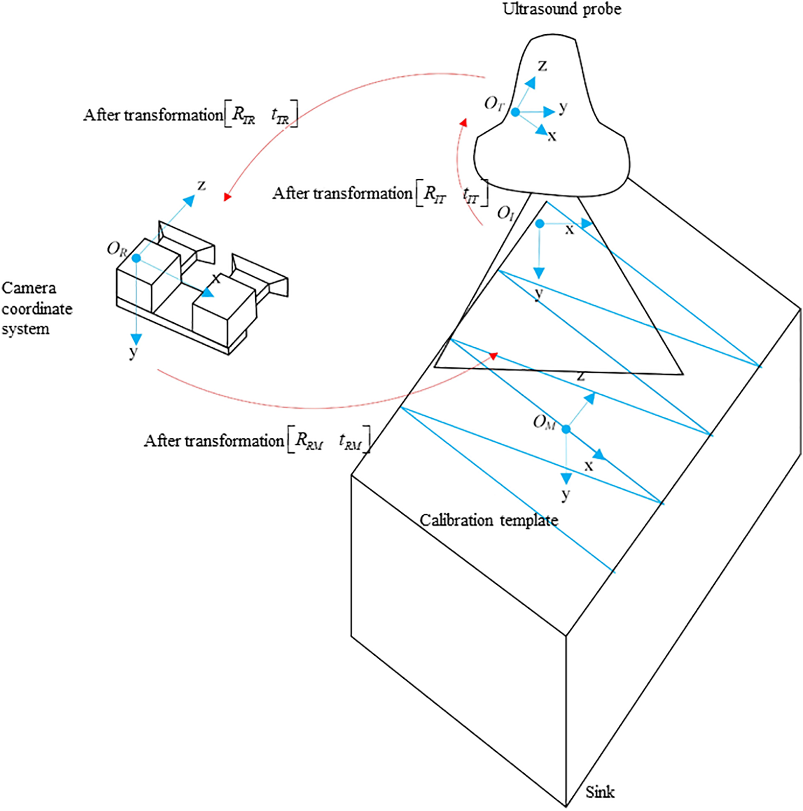
Figure 4: Calibration of ultrasound probes

We establish four coordinate systems: the template coordinate system OMXMYMZM, the camera coordinate system ORXRYRZR, the ultrasound probe coordinate system OTXTYTZT, and the ultrasound image coordinate system OIXIYIZI. Subsequently, we determine the conversion matrices: matrix [RRMtRM] for transforming the camera coordinate system to the template coordinate system, matrix [RTRtTR] for converting the probe coordinate system to the camera coordinate system, and matrix [RITtIT] for the transformation of the image coordinate system to the probe coordinate system.

Therefore, after obtaining the feature point’s coordinates pm in the template coordinate system and pi in the ultrasound image’s coordinate system, the calibration Eq. (21) can be derived as follows.

[pm1]=[RRMtRM01][RTRtTR01][RITtIT01][pi1](21)

where pm=[XM,YM,ZM]T is the homogeneous coordinate of the feature point in the template coordinate system. In pi=[Sxu,Syv,0,1]T, Sx is the resolution of the ultrasound image in the X-axis direction, Sy is the resolution in the Y-axis direction of the ultrasound image, and Sx, Sy is the unknown scale factor to be calibrated. u and v represent the pixel coordinates of the X- and Y-axis of the ultrasound image. The transformation matrix [RRMtRM], [RTRtTR] are 3×4 dimensional matrices that can be obtained by optical positioning devices, [RITtIT] is the transformation matrix to be calibrated, including tx,ty,tz,α,β,γ, as shown in Eqs. (22) and (23).

RlT=[cos⁡α×cos⁡βcos⁡α×sin⁡β×sin⁡γ−sin⁡α×cos⁡γcos⁡α×sin⁡β×cos⁡γ+sin⁡α×sin⁡γsin⁡α×cos⁡βsin⁡α×sin⁡β×sin⁡γ+cos⁡α×cos⁡γsin⁡α×sin⁡β×cos⁡γ−cos⁡α×sin⁡γ−sin⁡βcos⁡β×sin⁡γcos⁡β×cos⁡γ](22)

tIT=[txtytz](23)

The above expression indicates that the ultrasound image calibration requires solving for 6 calibration parameters along with Sx and Sy, totaling 8 unknown calibration parameters. Using the previously developed binocular visual tracking system and the ultrasound guidance bracket, we ensure that the calibration feature points are precisely captured within the scanning field of the ultrasound probe. This guarantees the accurate acquisition of two-dimensional ultrasound image data for the calibration points, which is crucial for precise calibration and subsequent navigation processes. Additionally, the coordinates of the calibration landmarks within the camera’s reference frame can be directly determined using calibration devices, thus eliminating the need for template calibration procedures.

Eq. (21) is simplified as Eq. (24).

[pr1]=[RTRtTR01][RITtIT01][pi1](24)

where pr is the coordinate of the feature point in the camera system, given by [Xr,Yr,Zr]T. pi is the intersection point of a line in the two-dimensional ultrasound image with an N-line model. The endpoints of this line can be calibrated in the camera model using the puncture needle tip model, denoted as [X1,Y1,Z1],[X2,Y2,Z2]. Subsequently, the corresponding linear equation is presented in Eq. (25).

Xr−X1X2−X1=Yr−Y1Y2−Y1=Zr−Z1Z2−Z1(25)

Then Xr, Yr can be expressed as Eq. (26).

Xr=(X2−X1)Zr−Z1X2+Z2X1Z2−Z1

Yr=(Y2−Z1)Zr−Z1Y2+Z2Y1Z2−Z1(26)

Substituting pr,pi into Eq. (24) yields the following Eq. (27).

[XrYrZr1]=[RTRtTR01][RITtIT01][SxuSyu01](27)

Substituting [RITtIT] into the above Eq. (27) yields Eq. (28).

[XrYrZr1]=[RTRtTR01][cos⁡α×cos⁡βT1T2txsin⁡α×cos⁡βT3T4ty−sin⁡βcos⁡β×sin⁡γcos⁡β×cos⁡γtz0001][SxuSyu01]

T1=cos⁡αsin⁡βsin⁡γ−sin⁡αcos⁡γT2=cos⁡αsin⁡βcos⁡γ+sin⁡αsin⁡γT3=sin⁡αsin⁡βsin⁡γ+cos⁡αcos⁡γT4=sin⁡αsin⁡βcos⁡γ−cos⁡αsin⁡γ(28)

It is evident that when the number of calibration ultrasound images M satisfies the condition 2M≥8, the unknown parameters can be determined using the appropriate mathematical analysis method.

To determine the calibration parameters using the nonlinear optimization method, the objective function is first formulated. For the calibration feature points of each image, Eq. (29) is used.

[RTRtTR01][RIT(i)tIT(i)01][SxuSyu01]=[Xr(j)Yr(j)Zr(j)1](29)

where i=1,2,…,M represents the ordinal number of the calibration image, and take L points per frame of an image, j=1,2,…,M, represents the j-th point. [RIT(i)tIT(i)] represents the rotational translation matrix of the i-th image coordinate system transformed into the coordinate system of the ultrasound transducer.

Then we have Eq. (30).

fj(ψ)=[fj(ψ)xfj(ψ)yfj(ψ)z1]=[RTRtTR01][RIT(i)tIT(i)01][SxuSyu01]−[Xr(j)Yr(j)Zr(j)1](30)

where ψ=[tx,ty,tz,α,β,γ,Sx,Sy]T, since fj(ψ)z has been used to solve the N-line equation, the objective function is constructed as Eq. (31).

fj(ψ)=[fj(ψ)xfj(ψ)yfj(ψ)z⋅⋅⋅fLM(ψ)xfLM(ψ)y](31)

The MSE of the distance deviation is Eq. (32).

EMSE=‖f(ψ)‖22(32)

The optimization problem for the goal is shown in Eq. (33).

ψ∗=arg⁡minψEMSE(33)

The above equation represents the optimization result, where the least squares method is employed in MATLAB to optimize the eight calibration parameters, aiming to minimize the values towards zero. In this study, the least squares method is utilized to solve systems of equations. When the EMSE is minimized, the initial tx,ty,tz,α,β,γ,Sx,Sy are substituted, and the function ψ is applied so that its partial derivative with respect to the eight parameters are equal to zero, as demonstrated in Eq. (34).

δEMSEδψ=δEMSEδ[tx,ty,tz,α,β,γ,Sx,Sy]T=0(34)

Then we can obtain the parameters tx^,ty^,tz^,α^,β^,γ^,Sx^,Sy^ of the calibration equation.

3  Experiments and Results

3.1 Instruments

3.1.1 Experimental Instruments for Needle Tip Calibration

The camera used in this study is a Medvision industrial camera model MV-MSU130GM2-T. The experimental setup includes four optical balls, a puncture needle, and a needle cover, as shown in Fig. 5.

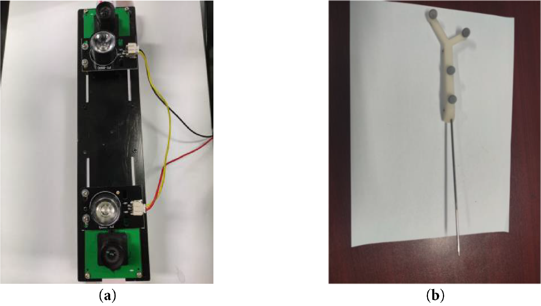
Figure 5: Experimental instrument structure diagram. (a) video camera; (b) puncture needle

The 3D-printed hub of the piercing needle contains four threaded holes designed to attach the optical balls. During the experiment, the camera captures images of these four optical balls attached to the puncture needle, and their coordinates are determined within the camera coordinate system using binocular positioning.

3.1.2 Experimental Instruments for Needle Tip Calibration

The ultrasound probe used in this experiment is a Sonostar all-digital ultrasound imaging diagnostic instrument, model CProbe. The camera employed is a Medvision industrial camera, model MV-MSU130GM2-T. The robotic arm utilized is the EC63, a lightweight 6-degree-of -freedom modular collaborative robot developed by Suzhou Elite Robot Co. Additional equipment includes ultrasound probe holders, optically marked pellets, N-type nylon wire, and a sink (filled with water maintained at 50°C). The configuration of the camera and the calibration board for the ultrasound probe is shown in Fig. 6.

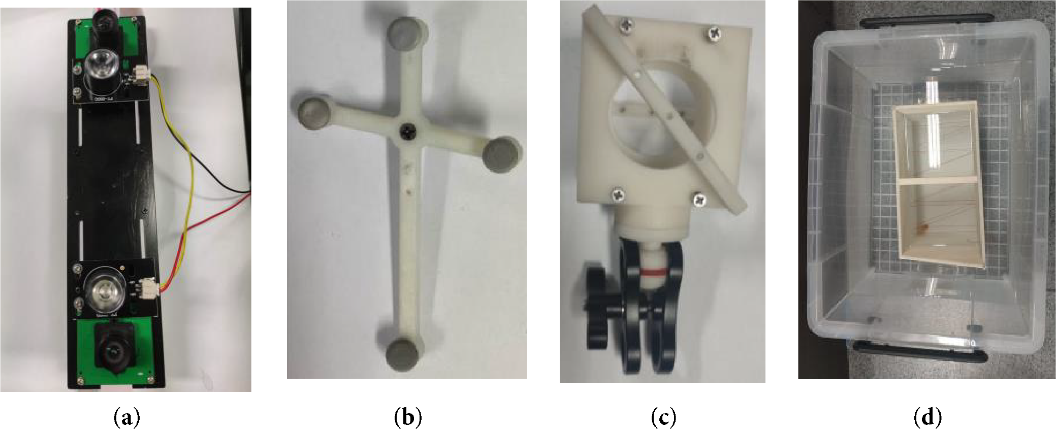
Figure 6: Schematic diagram of experimental equipment. (a) camera structure; (b) calibration plate structure; (c) fixture structure; (d) sink structure

3.2 Experiments on Needle Tip Calibration

During the experiment, the camera captures images of four optical spheres attached to the puncture needle, and their coordinates are determined in the camera’s coordinate system through using dual targeting. By rotating the puncture needle tip 130 degrees around the calibration plate, we obtained 253 image frames of the 4 optical balls, as depicted in Fig. 7.

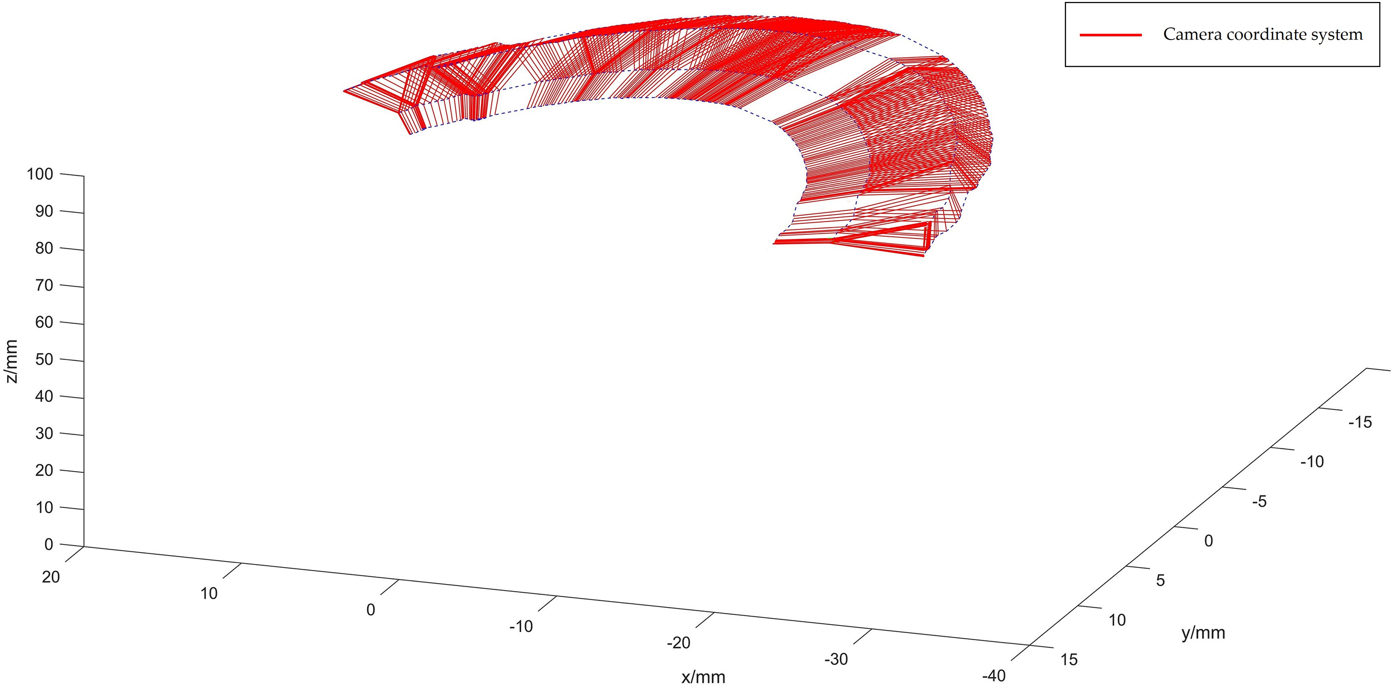
Figure 7: Optical sphere diagram in the camera coordinate system

The coordinates in the template coordinate system are determined using gradient descent, applied to the images captured under the 253-frame camera coordinate system, as depicted in Fig. 8.

Figure 8: Optical spherical diagram in template coordinate system

The spatial coordinates of the optical sphere, relative to the template coordinate system, are described in Eq. (35).

[PE1PE2PE3PE4]=[−2.92500−3.14650−2.47750−2.138858.21391.202731.082981.118409.408909.482689.290829.19578](35)

The spatial coordinates of the four optical spheres within the instrument’s reference coordinate system are described by Eq. (36).

[PD1PD2PD3PD4]=[−2.068051.982150.042950.04295−1.956775−3.8777752.9174256.4349250000](36)

The coordinates in the template coordinate system are converted to the instrument coordinate system using the optimal rotation algorithm, resulting in [REDtED].

Considering the error in the coordinate transformation obtained by the optimal rotation algorithm (e=0.0111mm), the coordinates of the optical sphere in the template coordinate system are adjusted using [REDtED] to align with the optimized instrument coordinate system, as shown in Fig. 9.

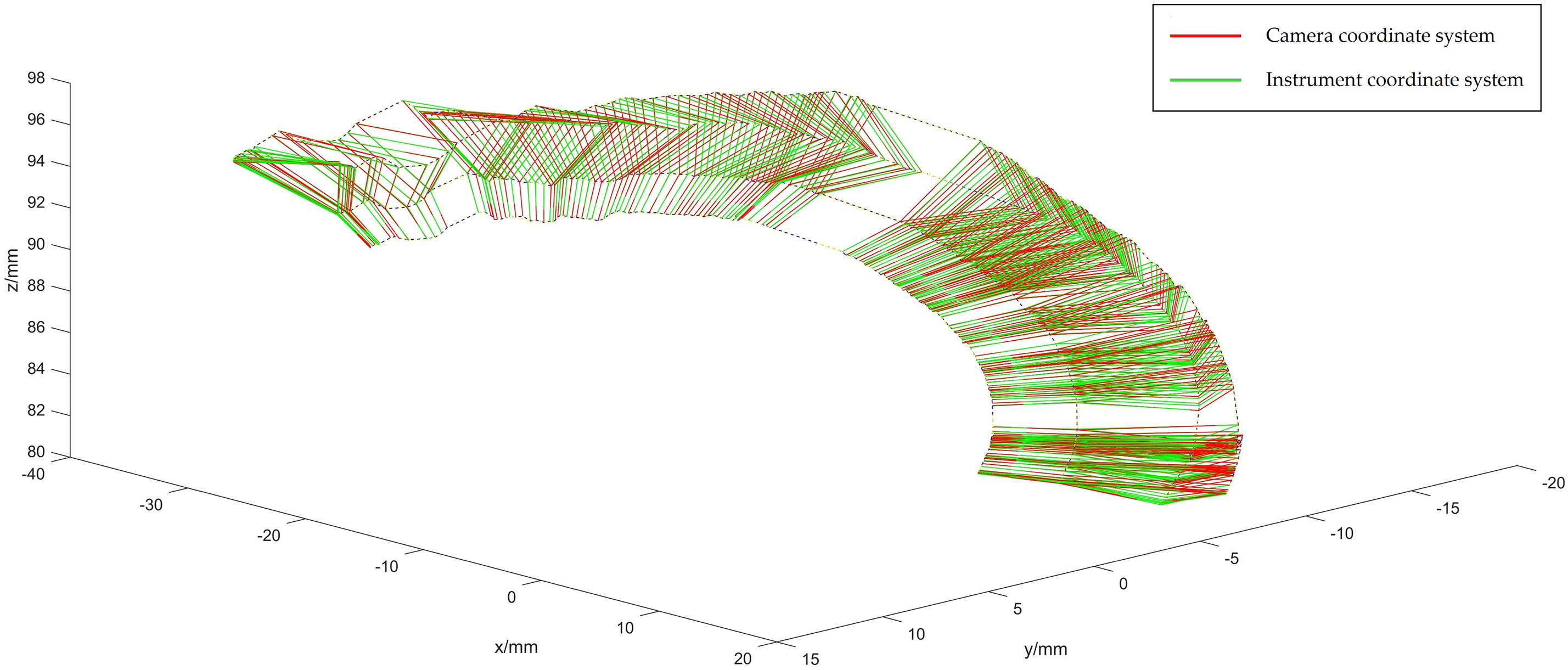
Figure 9: Optical spheroids of the optimized instrument coordinate system

The coordinates of the four optical spheres are presented in Eq. (37).

[PG1PG2PG3PG4]=[−2.06401.97510.05290.0360−1.9627−3.88232.91416.44880.00050.0006−0.00280.0018](37)

Using the optimal rotation algorithm, the coordinates of the optical spheres in the optimized instrument coordinate system are converted to the 253-frame camera coordinate system, allowing us to obtain the transformation matrix [REDtED],k=1,2,…,253.

The coordinate of the needle tip in the instrument coordinate system is PD0=[−0.33705,25.317425,−1.33], taking PG0≈PD0 in the optimized instrument coordinate system. Converting an endpoint of the optimized instrument coordinate system to a 253-frame image using the transformation matrix [RED(k)tED(k)] allows us to determine the coordinates of the optical sphere in the 253-frame camera coordinate system, as illustrated in Fig. 10.

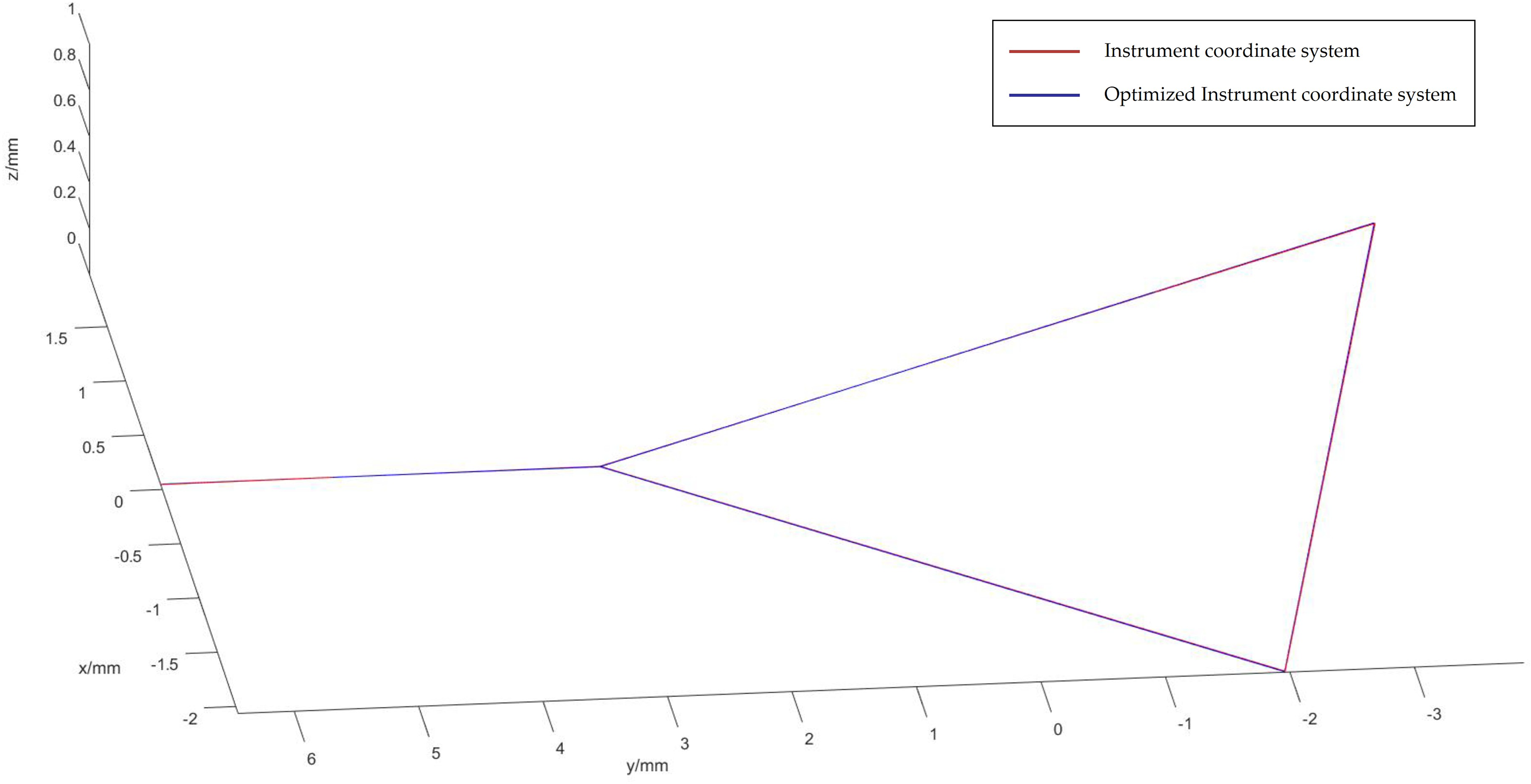
Figure 10: Optical spheroids of the optimized instrument coordinate system

The needle tip and optical sphere coordinates in the instrument coordinate system are transformed using [RED(k),tED(k)] to generate the corresponding image, as illustrated in Fig. 11.

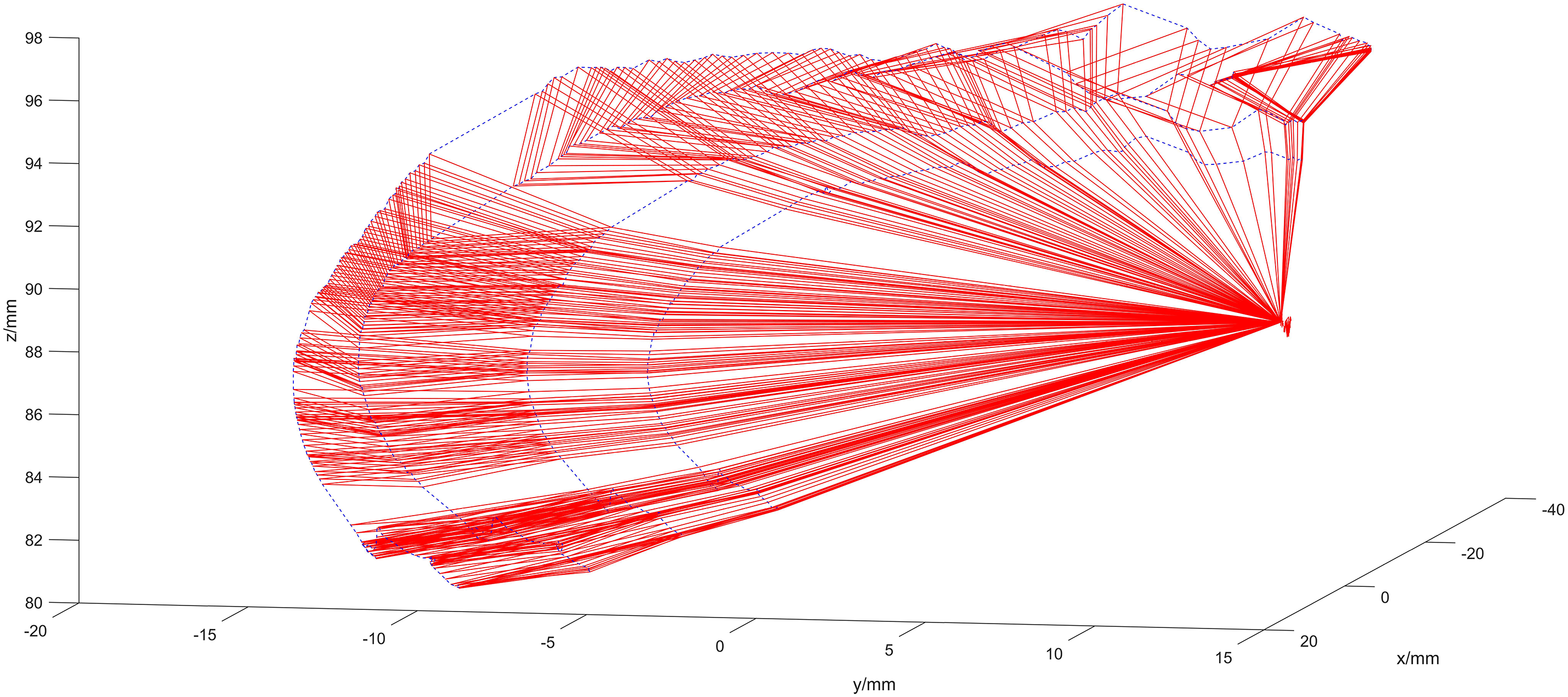
Figure 11: Optimized calibration scenario

The average offset distance of the four optical spheres per frame, across all 253-frames, is illustrated in Fig. 12.

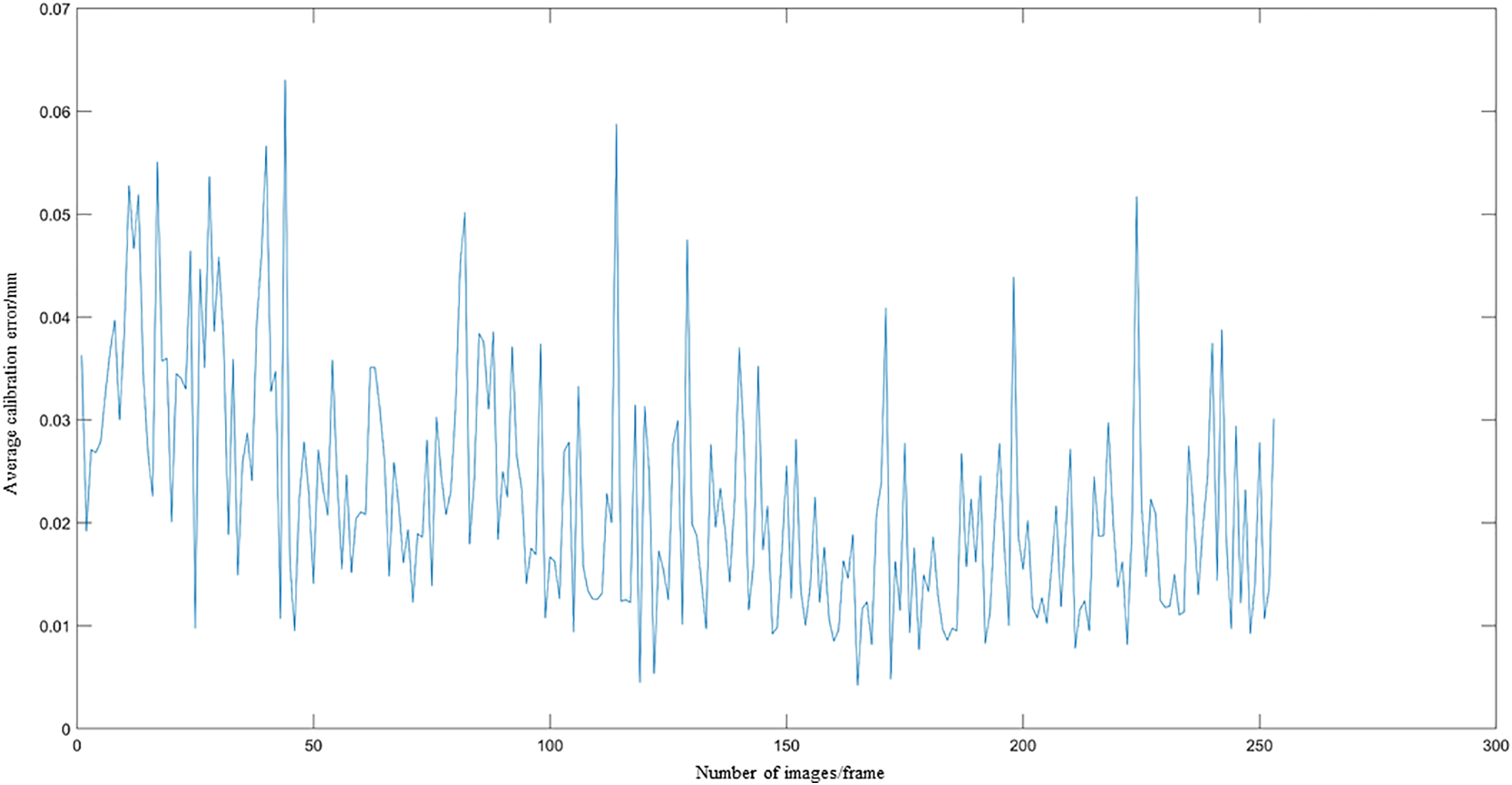
Figure 12: The average offset distance of the four optical spheroids

Fig. 13 illustrates the calibration error for the tip in each frame of the 253-frame sequence.

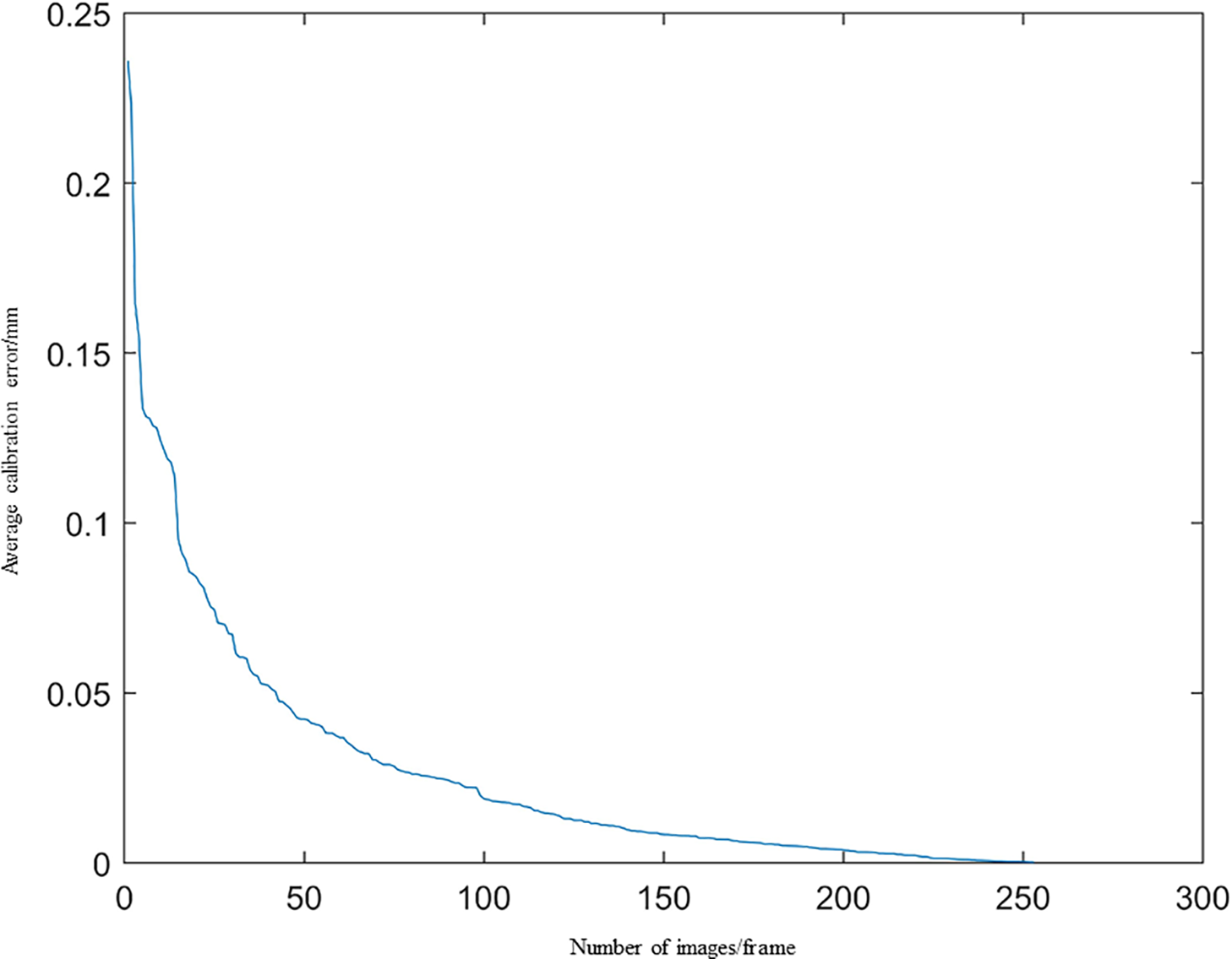
Figure 13: Calibration error diagram of the tip of the needle

Fig. 13 demonstrates a consistent decline in calibration error as the number of images increases, with deviations remaining below 0.25 mm throughout.

The gradient descent method is used to optimize the objective function based on 253 tip points, yielding an optimized coordinate for the puncture tip of [−0.333,25.2367,−1.2632]. Following this optimization, the calibration error of the tip is EMSE=0.1644mm. Thus, the experimentally obtained coordinates of the puncture tip are in close agreement with the estimated values.

3.3 Experiments with Ultrasound Probe Calibration

We take M = 30 ultrasound images, each containing L = 4 points. The coordinates of the two endpoints on the N-line are obtained, as shown in the resulting N-line image in Fig. 14.

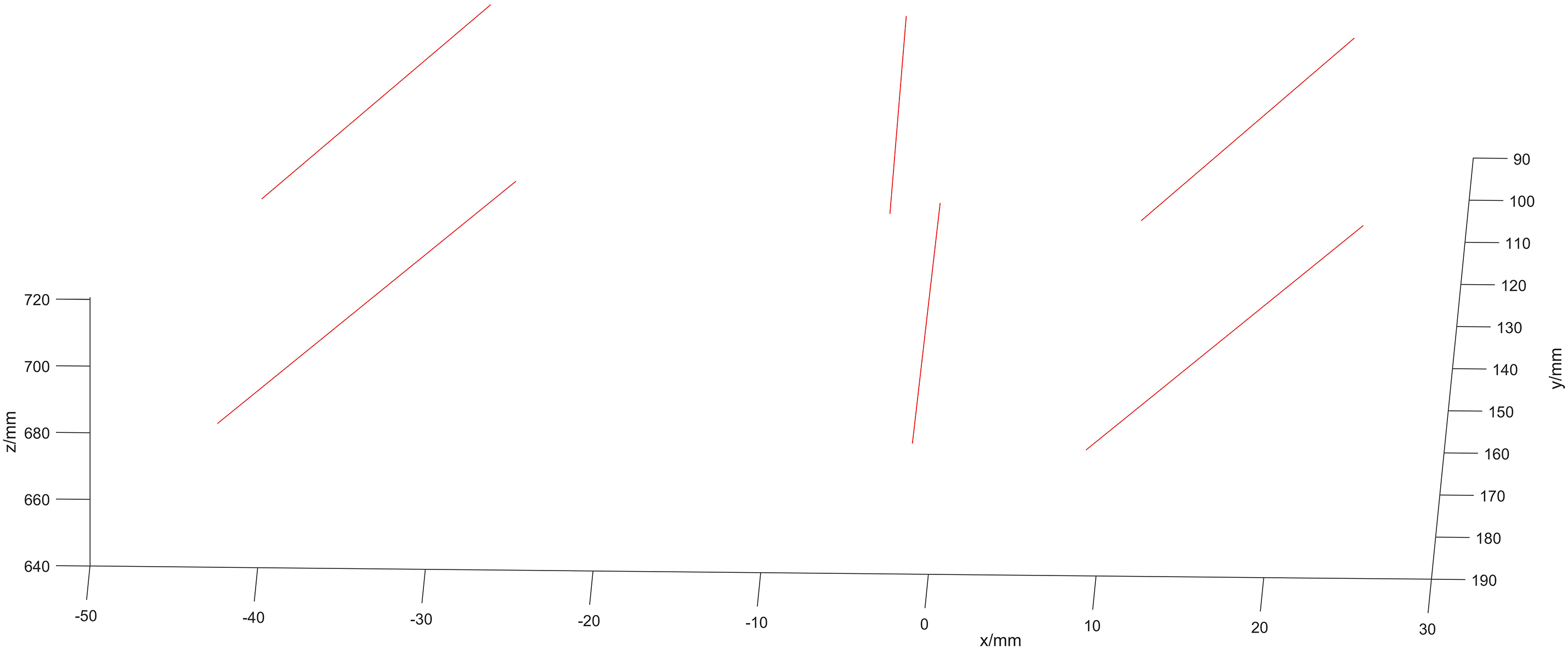
Figure 14: Image of the N-line

The spatial coordinates of the optical marker in the probe’s reference frame are described by Eq. (38):

T=[5.20970−5.209−30−29.544029.54400000](38)

Fig. 15 illustrates images of 30 sets of optical spheres held by the ultrasound probe.

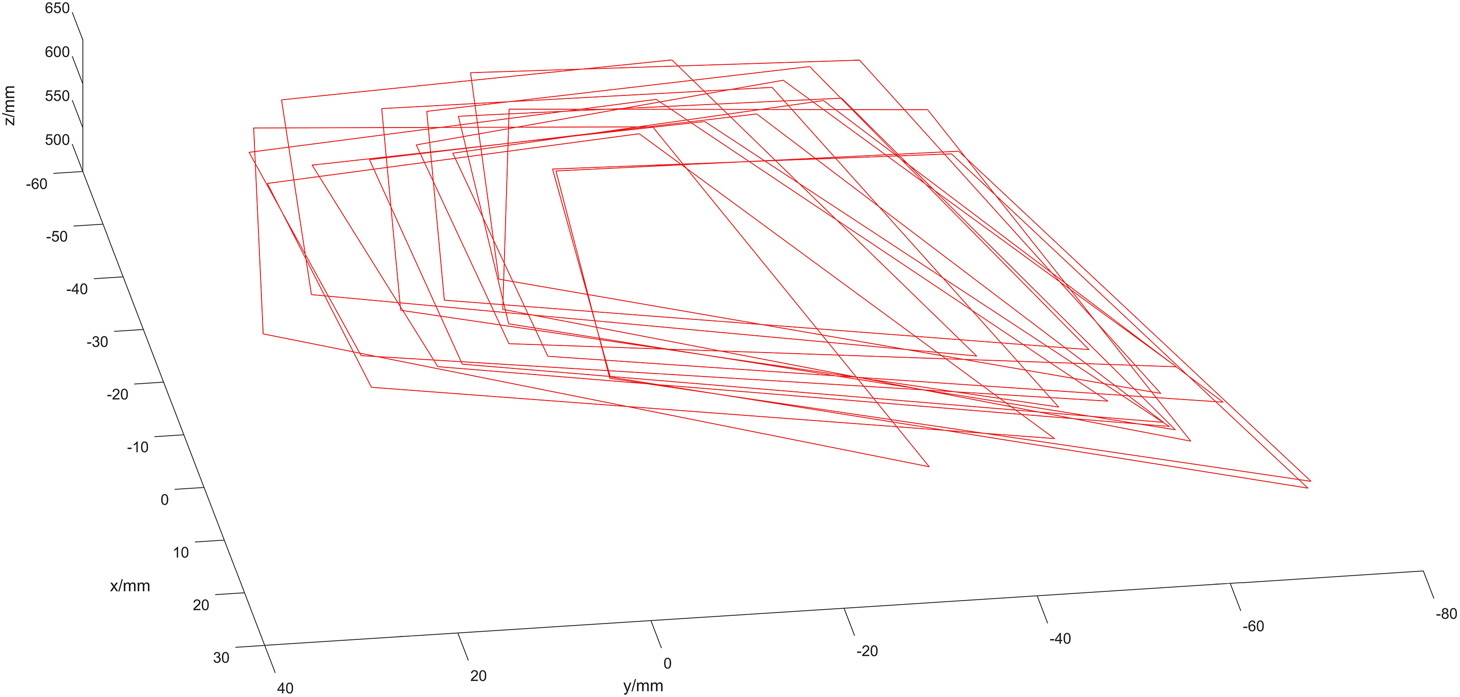
Figure 15: Optical spheroids in the camera’s coordinate system

Substituting the initial value [tx,ty,tz,α,β,γ,Sx,Sy]=[0.8,0,0,130,−90,−42,0.117,0.116], and calculating the optimized values using Eq. (38) yields: [tx^,ty^,tz^,α^,β^,γ^,Sx^,Sy^]=[0.7721,−0.1024,0.0455,136.1327,−90.2300,−39.3303,0.1277,0.1233].

Subsequently, the ultrasound image is transformed into the camera coordinate system, as shown in Fig. 16.

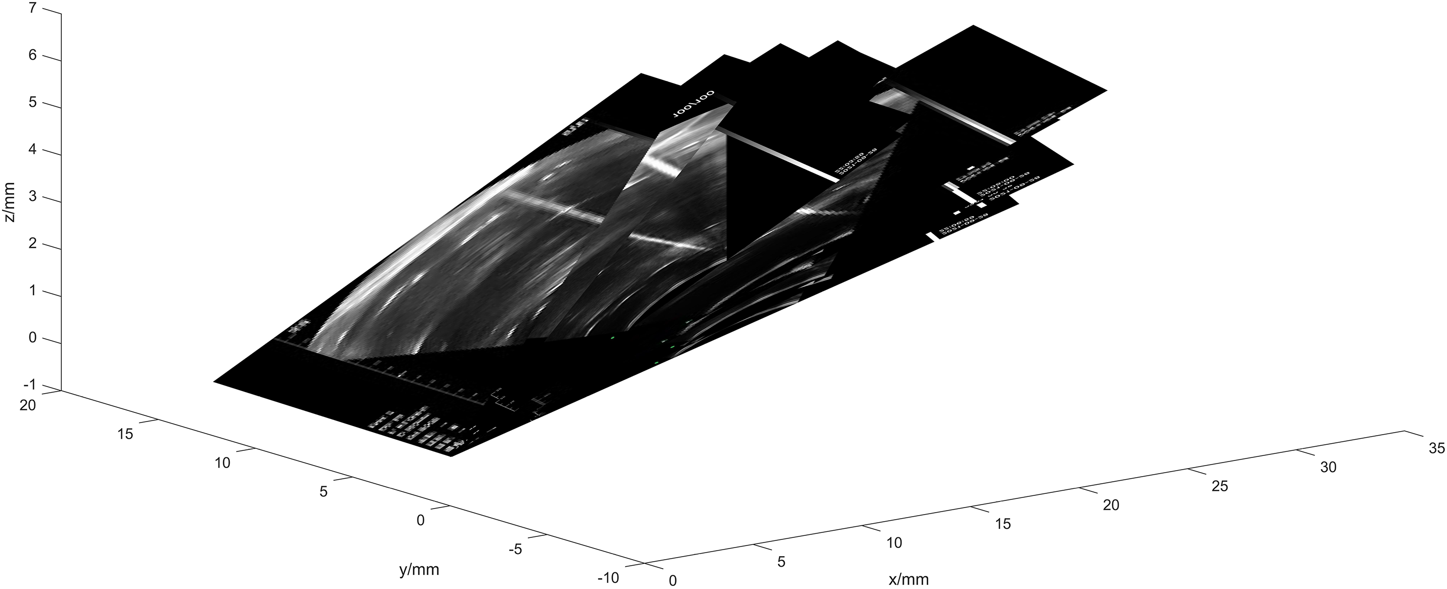
Figure 16: Schematic diagram of ultrasound probe calibration

Two points from the same side wall of the sink were selected from each frame image, and the resulting image of the pipe wall is illustrated in Fig. 17.

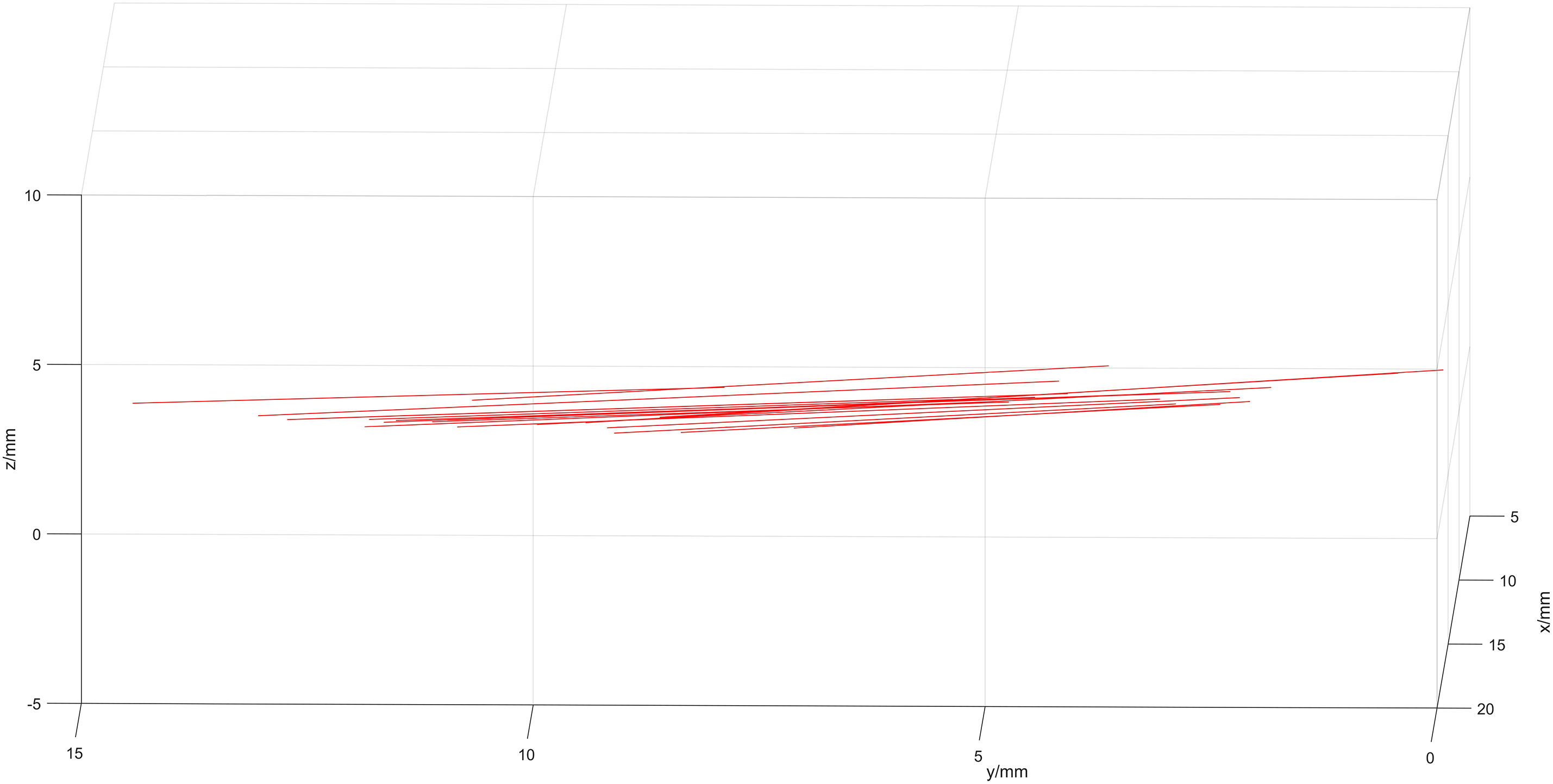
Figure 17: Image of the pipe wall

Fig. 17 shows that the pipe wall aligns closely with a single plane, with a deviation of less than 1 mm, thereby improving calibration precision. In this experiment, the value of EMSE is found to be 1.2373mm, indicating that the average displacement per pixel is 1.2373 mm. Despite potential errors during the calibration of the N-line model at the puncture tip and in solving the transformation matrix between coordinate systems, these inaccuracies are minimal and do not significantly affect the overall results.

4  Discussion

Surgical navigation systems have undergone rapid advancements in recent years, particularly in improving intraoperative precision and reducing patient trauma. Nevertheless, traditional navigation methods based on binocular stereovision often suffer from limited visibility in obstructed anatomical regions and lack robustness in dynamic scenarios [28,29]. To address these limitations, our approach integrates optical tracking, robotic manipulation, and real-time ultrasound guidance into a unified calibration framework.

A critical challenge in ultrasound-guided interventions is the accurate spatial registration between the ultrasound probe and the needle tip, which has typically been addressed in isolation. For instance, Kim et al. [30] proposed a calibration procedure for needle-guide systems attached to ultrasound probes, but their method relied on fixed mechanical assumptions and was not applicable to freehand scenarios. Similarly, Paralikar et al. [31] developed a robot-assisted calibration for the probe itself, but without considering the dynamic spatial behavior of the needle tip.

Other studies such as Carbajal et al. [32] utilized N-wire phantoms for ultrasound probe calibration, but treated needle localization as a separate or manually controlled process, introducing potential cumulative error. In contrast, our method achieves joint calibration, in which the accurately optimized needle tip coordinates are directly employed to solve the N-line model of the ultrasound probe. This integration ensures tighter spatial coupling, minimizes registration errors, and eliminates reliance on external fiducial phantoms.

Our experimental results demonstrate that this integrated approach significantly enhances calibration precision. The needle tip localization error remains under 0.25 mm across 253 captured frames, and the ultrasound probe calibration achieves a pixel deviation of only 1.2373 mm. Furthermore, the alignment of the calibrated ultrasound image with a known planar surface shows deviation below 1 mm, reinforcing the spatial accuracy of the proposed method. Compared to previous methods, this represents a substantial improvement in both accuracy and robustness under freehand or robotic setups.

In summary, the proposed joint calibration framework fills a notable gap in the current literature by unifying two previously separate procedures—needle tip and probe calibration—into a single optimization-based workflow. This method has strong potential for application in real-time surgical navigation, especially in 2D ultrasound-based systems that require precise spatial coordination without the aid of ionizing radiation.

Nevertheless, several limitations remain. The current experiments were conducted in a phantom environment using an optical tracking system, industrial camera, and robotic arm, we clarify that the proposed joint calibration method has not yet been deployed or tested on a fully integrated surgical navigation system in clinical or pre-clinical settings. The implementation was performed within a controlled prototype environment designed to simulate real-world constraints, including hardware synchronization and image acquisition workflows that align with those of standard navigation systems. In addition, while gradient descent with a fixed step size proved effective in our study, we acknowledge that more advanced optimization strategies, such as particle swarm optimization or other metaheuristic algorithms, may further enhance robustness in more complex or nonlinear calibration scenarios. Recent reviews and algorithmic studies on robot calibration highlight the effectiveness of data-driven and evolutionary approaches for improving optimization performance, which could inspire future extensions of our framework [33,34].

The entire calibration pipeline was implemented end-to-end, covering both needle tip localization and ultrasound probe-to-image registration. However, real-time integration into a functioning navigation system with user interface, intraoperative imaging, and surgeon feedback loop remains a direction for future development. The current results demonstrate the feasibility and internal consistency of the proposed model, providing a solid computational foundation for future system-level integration. We acknowledge that validation under more complex surgical conditions, such as soft tissue deformation, occlusion, or dynamic anatomical changes, will be necessary to demonstrate robustness in realistic environments. As such, future work will focus on extending the system to animal models or hybrid OR setups, and addressing practical challenges like tracking loss, calibration drift, and probe misalignment through sensor fusion and online error correction methods.

5  Conclusions

In this research, we introduce an advanced method for precise needle tip localization using a sophisticated rotation algorithm. This technique involves rotating the needle tip by 130 degrees around a fixed pivot, which enables the acquisition of multiple images of four optical spheres within the camera’s coordinate system. These images are then employed to refine the template coordinate system through gradient descent optimization. Subsequently, the coordinates within the template system are transformed into the instrument’s coordinate system. Further optimization of these coordinates is performed within the camera’s coordinate system. Notably, as the number of captured images increases, the calibration error remains consistently low, demonstrating remarkable stability and accuracy.

We then utilize the optimized needle tip coordinates to develop a joint calibration algorithm for the ultrasound probe. This calibration involves identifying the two endpoints of each N-line using the calibrated needle tip and solving the N-line equations based on ultrasound images. Additionally, using data from optical spheres captured by the optical positioning framework, we derive a transformation matrix to facilitate the transition from the probe’s reference system to the camera’s coordinate system. The calibration matrix for the ultrasound probe is formulated using a least-squares methodology, ensuring an optimized solution.

In our experimental setup, we used a Sonostar digital ultrasound imaging system equipped with a CProbe probe. The camera used was the MV-MSU130GM2-T industrial camera from MedViewTech. The mechanical arm used in the experiments was the EC63 intelligent lightweight 6-degree-of-freedom modular collaborative robot developed by Suzhou Eletech Robotics Co. Our experimental results validate the proposed method’s efficacy in achieving high-precision calibration for 2D ultrasound surgical navigation, showing stable calibration errors across different numbers of images.

Overall, the study establishes a practical and accurate calibration strategy that addresses a long-standing gap in ultrasound-guided navigation, offering a streamlined workflow with potential for translation into real-time minimally invasive surgical applications.

Acknowledgement: None.

Funding Statement: Support by Sichuan Science and Technology Program [2023YFSY0026, 2023YFH0004].

Author Contributions: The authors confirm contribution to the paper as follows: conceptualization, Bo Yang and Shan Liu; methodology, Bo Yang and Fupei Guo; software, Bo Yang and Xiang Zhang; validation, Jiawei Tian and Yu Zhou; formal analysis, Fupei Guo; investigation, Xiang Zhang; resources, Jiawei Tian; data curation, Xiang Zhang; writing—original draft preparation, Bo Yang; writing—review and editing, Jiawei Tian; visualization, Yu Zhou; supervision, Jiawei Tian; project administration, Shan Liu; funding acquisition, Shan Liu. All authors reviewed the results and approved the final version of the manuscript.

Availability of Data and Materials: All data generated or analyzed during this study are included in this published article.

Ethics Approval: Not applicable.

Conflicts of Interest: The authors declare no conflicts of interest to report regarding the present study.

References

1. Recker F, Höhne E, Damjanovic D, Schäfer VS. Ultrasound in telemedicine: a brief overview. Appl Sci. 2022;12(3):958. doi:10.3390/app12030958. [Google Scholar] [CrossRef]

2. Chandrashekhara SH, Rangarajan K, Agrawal A, Thulkar S, Gamanagatti S, Raina D, et al. Robotic ultrasound: an initial feasibility study. World J Methodol. 2022;12(4):274–84. doi:10.5662/wjm.v12.i4.274. [Google Scholar] [CrossRef]

3. Elmi-Terander A, Burström G, Nachabe R, Skulason H, Pedersen K, Fagerlund M, et al. Pedicle screw placement using augmented reality surgical navigation with intraoperative 3D imaging: a first in-human prospective cohort study. Spine. 2019;44(7):517–25. doi:10.1097/brs.0000000000002876. [Google Scholar] [PubMed] [CrossRef]

4. Gonzalez LV, Arango A, López JP, Gnecco JP. Technological integration of virtual surgical planning, surgical navigation, endoscopic support and patient-specific implant in orbital trauma. J Maxillofac Oral Surg. 2021;20(3):459–63. doi:10.1007/s12663-020-01423-x. [Google Scholar] [CrossRef]

5. Lartizien R, Zaccaria I, Savoldelli C, Noyelles L, Chamorey E, Cracowski JL, et al. Learning condyle repositioning during orthognathic surgery with a surgical navigation system. Int J Oral Maxillofac Surg. 2019;48(7):952–6. doi:10.1016/j.ijom.2019.01.018. [Google Scholar] [PubMed] [CrossRef]

6. Quang TT, Chen WF, Papay FA, Liu Y. Dynamic, real-time, fiducial-free surgical navigation with integrated multimodal optical imaging. IEEE Photonics J. 2021;13(1):1–13. doi:10.1109/jphot.2020.3042269. [Google Scholar] [CrossRef]

7. Granata A, Distefano G, Pesce F, Battaglia Y, Suavo Bulzis P, Venturini M, et al. Performing an ultrasound-guided percutaneous needle kidney biopsy: an up-to-date procedural review. Diagnostics. 2021;11(12):2186. doi:10.3390/diagnostics11122186. [Google Scholar] [PubMed] [CrossRef]

8. Lee JY, Islam M, Woh JR, Mohamed Washeem TS, Ngoh LYC, Wong WK, et al. Ultrasound needle segmentation and trajectory prediction using excitation network. Int J Comput Assist Radiol Surg. 2020;15(3):437–43. doi:10.1007/s11548-019-02113-x. [Google Scholar] [PubMed] [CrossRef]

9. Gueziri HE, Drouin S, Yan CXB, Collins DL. Toward real-time rigid registration of intra-operative ultrasound with preoperative CT images for lumbar spinal fusion surgery. Int J Comput Assist Radiol Surg. 2019;14(11):1933–43. doi:10.1007/s11548-019-02020-1. [Google Scholar] [PubMed] [CrossRef]

10. Jengojan S, Sorgo P, Streicher J, Snoj Ž, Kasprian G, Gruber G, et al. Ultrasound-guided thread versus ultrasound-guided needle release of the A1 pulley: a cadaveric study. Radiol Med. 2024;129(10):1513–21. doi:10.1007/s11547-024-01875-y. [Google Scholar] [PubMed] [CrossRef]

11. Li Q, Lin X, Zhang X, Samir AE, Arellano RS. Imaging-related risk factors for bleeding complications of US-guided native renal biopsy: a propensity score matching analysis. J Vasc Interv Radiol. 2019;30(1):87–94. doi:10.1016/j.jvir.2018.08.031. [Google Scholar] [PubMed] [CrossRef]

12. Edwards W, Tang G, Tian Y, Draelos M, Izatt J, Kuo A, et al. Data-driven modelling and control for robot needle insertion in deep anterior lamellar keratoplasty. IEEE Robot Autom Lett. 2022;7(2):1526–33. doi:10.1109/lra.2022.3140458. [Google Scholar] [PubMed] [CrossRef]

13. Hong A, Petruska AJ, Zemmar A, Nelson BJ. Magnetic control of a flexible needle in neurosurgery. IEEE Trans Biomed Eng. 2021;68(2):616–27. doi:10.1109/tbme.2020.3009693. [Google Scholar] [PubMed] [CrossRef]

14. Jiang Y, Song Q, Gao F, Liu Z, Gupta MK, Hao X. Needle deformation in the process of puncture surgery: experiment and simulation. Procedia CIRP. 2020;89(3):270–6. doi:10.1016/j.procir.2020.05.151. [Google Scholar] [CrossRef]

15. Zhong F, Wang Z, Chen W, He K, Wang Y, Liu YH. Hand-eye calibration of surgical instrument for robotic surgery using interactive manipulation. IEEE Robot Autom Lett. 2020;5(2):1540–7. doi:10.1109/lra.2020.2967685. [Google Scholar] [CrossRef]

16. Pavone M, Seeliger B, Teodorico E, Goglia M, Taliento C, Bizzarri N, et al. Ultrasound-guided robotic surgical procedures: a systematic review. Surg Endosc. 2024;38(5):2359–70. doi:10.1007/s00464-024-10772-4. [Google Scholar] [PubMed] [CrossRef]

17. van Boxel GI, Carter NC, Fajksova V. Three-arm robotic cholecystectomy: a novel, cost-effective method of delivering and learning robotic surgery in upper GI surgery. J Robot Surg. 2024;18(1):180. doi:10.1007/s11701-024-01919-5. [Google Scholar] [PubMed] [CrossRef]

18. Beigi P, Salcudean SE, Ng GC, Rohling R. Enhancement of needle visualization and localization in ultrasound. Int J Comput Assist Radiol Surg. 2021;16(1):169–78. doi:10.1007/s11548-020-02227-7. [Google Scholar] [PubMed] [CrossRef]

19. Wang KJ, Chen CH, Lo CY, Lin HH, Jason Chen JJ. Ultrasound calibration for dual-armed surgical navigation system. J Healthc Eng. 2022;2022:3362495. doi:10.1155/2022/3362495. [Google Scholar] [PubMed] [CrossRef]

20. Seitel A, Groener D, Eisenmann M, Aguilera Saiz L, Pekdemir B, Sridharan P, et al. Miniaturized electromagnetic tracking enables efficient ultrasound-navigated needle insertions. Sci Rep. 2024;14(1):14161. doi:10.1038/s41598-024-64530-6. [Google Scholar] [PubMed] [CrossRef]

21. Che H, Qin J, Chen Y, Ji Z, Yan Y, Yang J, et al. Improving needle tip tracking and detection in ultrasound-based navigation system using deep learning-enabled approach. IEEE J Biomed Health Inform. 2024;28(5):2930–42. doi:10.1109/JBHI.2024.3353343. [Google Scholar] [PubMed] [CrossRef]

22. Chai Z, Sun Y, Xiong Z. A novel method for LiDAR camera calibration by plane fitting. In: 2018 IEEE/ASME International Conference on Advanced Intelligent Mechatronics (AIM); 2018 Jul 9–12; Auckland, New Zealand. p. 286–91. doi:10.1109/aim.2018.8452339. [Google Scholar] [CrossRef]

23. Nurbekyan L, Lei W, Yang Y. Efficient natural gradient descent methods for large-scale PDE-based optimization problems. SIAM J Sci Comput. 2023;45(4):A1621–55. doi:10.1137/22m1477805. [Google Scholar] [CrossRef]

24. Masood H, Zafar A, Ali MU, Hussain T, Khan MA, Tariq U, et al. Tracking of a fixed-shape moving object based on the gradient descent method. Sensors. 2022;22(3):1098. doi:10.3390/s22031098. [Google Scholar] [PubMed] [CrossRef]

25. Sorriento A, Porfido MB, Mazzoleni S, Calvosa G, Tenucci M, Ciuti G, et al. Optical and electromagnetic tracking systems for biomedical applications: a critical review on potentialities and limitations. IEEE Rev Biomed Eng. 2019;13:212–32. doi:10.1109/rbme.2019.2939091. [Google Scholar] [PubMed] [CrossRef]

26. Dai H, Zeng Y, Wang Z, Lin H, Lin M, Gao H, et al. Prior knowledge-based optimization method for the reconstruction model of multicamera optical tracking system. IEEE Trans Automat Sci Eng. 2020;17(4):2074–84. doi:10.1109/tase.2020.2989194. [Google Scholar] [CrossRef]

27. Song X, Zhang Y, Wang C, Zhao H, Liu A. Study on calibration method of ultrasonic probe based on electromagnetic positioner in puncture surgical robot. In: Proceedings of the 2022 4th International Conference on Robotics, Intelligent Control and Artificial Intelligence; 2022 Dec 16–18; Dongguan, China. p. 161–4. doi:10.1145/3584376.3584404. [Google Scholar] [CrossRef]

28. Teatini A, Kumar RP, Elle OJ, Wiig O. Mixed reality as a novel tool for diagnostic and surgical navigation in orthopaedics. Int J Comput Assist Radiol Surg. 2021;16(3):407–14. doi:10.1007/s11548-020-02302-z. [Google Scholar] [PubMed] [CrossRef]

29. Bi S, Wang M, Zou J, Gu Y, Zhai C, Gong M. Dental implant navigation system based on trinocular stereo vision. Sensors. 2022;22(7):2571. doi:10.3390/s22072571. [Google Scholar] [PubMed] [CrossRef]

30. Kim C, Chang D, Petrisor D, Chirikjian G, Han M, Stoianovici D. Ultrasound probe and needle-guide calibration for robotic ultrasound scanning and needle targeting. IEEE Trans Biomed Eng. 2013;60(6):1728–34. doi:10.1109/TBME.2013.2241430. [Google Scholar] [PubMed] [CrossRef]

31. Paralikar A, Mantripragada P, Nguyen T, Arjoune Y, Shekhar R, Monfaredi R. Robot-assisted ultrasound probe calibration for image-guided interventions. Int J Comput Assist Radiol Surg. 2025;20(5):859–68. doi:10.1007/s11548-025-03347-8. [Google Scholar] [PubMed] [CrossRef]

32. Carbajal G, Lasso A, Gómez Á, Fichtinger G. Improving N-wire phantom-based freehand ultrasound calibration. Int J Comput Assist Radiol Surg. 2013;8(6):1063–72. doi:10.1007/s11548-013-0904-9. [Google Scholar] [PubMed] [CrossRef]

33. Chen T, Yang W, Li S, Luo X. Data-driven calibration of industrial robots: a comprehensive survey. IEEE/CAA J Autom Sinica. 2025;12(8):1544–67. doi:10.1109/jas.2025.125237. [Google Scholar] [CrossRef]

34. Chen T, Li S, Qiao Y, Luo X. A robust and efficient ensemble of diversified evolutionary computing algorithms for accurate robot calibration. IEEE Trans Instrum Meas. 2024;73(6):7501814. doi:10.1109/TIM.2024.3363783. [Google Scholar] [CrossRef]