
 Submit a Paper
 Propose a Special lssue
 Open Access
ARTICLE

A Unified Parametric Divergence Operator for Fermatean Fuzzy Environment and Its Applications in Machine Learning and Intelligent Decision-Making
1 College of Mathematics and Computer, Xinyu University, Xinyu, 338004, China
2 School of Computer Sciences, Universiti Sains Malaysia, Penang, 11800, Malaysia
3 Jadara Research Center, Jadara University, Irbid, 21110, Jordan
4 Department of Applied Mathematics and Statistics, Johns Hopkins University, Baltimore, MD 21218, USA
5 School of Mathematics and Statistics, Southwest University, Chongqing, 400715, China
6 Saveetha School of Engineering, Saveetha Institute of Medical and Technical Sciences, Chennai, 602105, India
7 Centre for Research Impact & Outcome, Chitkara University Institute of Engineering and Technology, Chitkara University, Rajpura, 140401, India
8 Department of Electronic Engineering, Shanghai Jiao Tong University, Shanghai, 200240, China
9 Technology and Applied Sciences Laboratory, U.I.T. of Douala, University of Douala, Douala, P.O. Box 8689, Cameroon
10 Department of Applied Sciences, Advanced Centre of Research and Innovation, Chandigarh Engineering College, Chandigarh Group of Colleges, Jhanjeri, Mohali, 140307, India
11 School of Engineering & Technology, Duy Tan University, Da Nang, 550000, Vietnam
12 Department of AI, School of Computer Science and Engineering, Galgotias University, Greater Noida, 203201, India
* Corresponding Authors: Zhe Liu. Email: ; Yulong Huang. Email:
; Mehdi Hosseinzadeh. Email:
(This article belongs to the Special Issue: Algorithms, Models, and Applications of Fuzzy Optimization and Decision Making)
Computer Modeling in Engineering & Sciences 2025, 145(2), 2157-2188. https://doi.org/10.32604/cmes.2025.072352
Received 25 August 2025; Accepted 10 October 2025; Issue published 26 November 2025
 View Full Text
 Download PDF
Abstract
Uncertainty and ambiguity are pervasive in real-world intelligent systems, necessitating advanced mathematical frameworks for effective modeling and analysis. Fermatean fuzzy sets (FFSs), as a recent extension of classical fuzzy theory, provide enhanced flexibility for representing complex uncertainty. In this paper, we propose a unified parametric divergence operator for FFSs, which comprehensively captures the interplay among membership, non-membership, and hesitation degrees. The proposed operator is rigorously analyzed with respect to key mathematical properties, including non-negativity, non-degeneracy, and symmetry. Notably, several well-known divergence operators, such as Jensen-Shannon divergence, Hellinger distance, and χ2-divergence, are shown to be special cases within our unified framework. Extensive experiments on pattern classification, hierarchical clustering, and multiattribute decision-making tasks demonstrate the competitive performance and stability of the proposed operator. These results confirm both the theoretical significance and practical value of our method for advanced fuzzy information processing in machine learning and intelligent decision-making.Keywords
Dealing with imperfect information is a common task in everyday life, as uncertainty and ambiguity inevitably permeate any real-world system, creating challenges in the decision-making process [1,2]. Whether it is selecting the best alternative in business, diagnosing medical conditions, or making strategic decisions in engineering or finance, decision-makers are often confronted with complex situations where data is incomplete, imprecise, or ambiguous [3]. In such cases, conventional methods that rely on precise numerical values may fall short. To solve this problem, various effective theories have been established, like fuzzy sets [4,5], rough sets [6,7], Z-numbers [8,9], and Evidence theory [10,11]. These theories have a wide range of applications in various domains, such as supplier selection [12], decision-making [3], risk analysis [13], and medical diagnosis [14].
Among them, fuzzy sets, introduced by Zadeh [15], have become a foundational concept in modeling uncertainty. The notion of fuzzy sets allows for the representation of vague concepts by assigning a membership degree (MD) to elements in a set, providing a flexible way to handle ambiguous information. However, the classical fuzzy sets still face limitations when dealing with more complex uncertainty. Intuitionistic fuzzy sets (IFSs), developed by Atanassov [16], extended fuzzy sets by introducing a nonmembership degree (ND) along with the MD, providing a more comprehensive model of uncertainty. However, IFSs impose a strict constraint where the sum of the MD and ND must be less than or equal to one. This restriction can be limiting when dealing with high levels of ambiguity, as it fails to fully account for situations where both degrees exhibit substantial uncertainty. Building on IFSs, Pythagorean fuzzy sets (PFSs), introduced by Yager [17], offer a more flexible framework. PFSs allow the sum of the squares of the MD and ND to be less than or equal to one, relaxing the constraint imposed by IFSs. This relaxation provides more flexibility in modeling uncertainty and has attracted research focused on the application of PFSs [18,19]. Recently, Senapati and Yager [20] introduced Fermatean fuzzy sets (FFSs), which offer a further generalization by relaxing the constraints of IFSs and PFSs. FFSs use a more generalized relationship between the MD and ND, where the sum of the cubes of the MD and ND must be less than or equal to one. This generalized structure allows FFS to capture a broader range of uncertainty, making them highly suitable for decision-making scenarios that involve significant ambiguity and conflicting information. So far, FFS has attracted a lot of attention [21–23]. For example, Ref. [21] introduced several Fermatean fuzzy weighted average, weighted geometric, weighted power average, and weighted power geometric operators and applied them for the multiattribute decision-making (MADM) problem. Kakati et al. [22] suggested Fermatean fuzzy Archimedean Heronian mean and geometric Heronian mean operators, and developed a new MADM method for sustainable urban transport.
In practical applications, especially in fields involving pattern classification, clustering, decision-making, and artificial intelligence, measuring the discrepancy between two sets is crucial. Interestingly, distance/divergence/similarity operators for IFSs and PFSs have received great attention, and many operators have been developed. For example, some researchers have extended several widely used operators, including Hamming distance [24,25], Euclidean distance [24,26], Hausdorff distance [27,28], Jensen-Shannon divergence [29–31], Hellinger distance [32,33], cosine similarity [34,35], Jaccard similarity [36,37] and Dice similarity [38], to the environments of IFSs and PFSs, and have validated their effectiveness in scenarios such as pattern recognition, multiattribute decision-making (MADM) and medical diagnosis. Furthermore, more innovative distance and similarity operators for IFSs and PFSs can be found in the literature [39–41]. Several operators of distance and similarity have been developed for FFSs to enhance their practical utility. For example, Senapati and Yager [20] first introduced a Fermatean fuzzy operator based on Euclidean distance. Later, Onyeke and Ejegwa [42] pointed out that Senapati and Yager’s work contradicts the axiomatic of distance, and developed an enhanced distance operator for FFSs. Sahoo [43] introduced several similarity operators for FFSs and applied them to group decision-making. Kirisci [44] combined cosine similarity and Euclidean distance operators for FFSs, applying these concepts within the TOPSIS framework. Subsequently, lIU [45] highlighted deficiencies in Kirisci’s approach and introduced an improved cosine similarity operator. Ref. [46] designed the Hellinger distance and the triangular divergence for FFSs, respectively. Liu [14] proposed a new triangular divergence operator for FFSs to overcome the limitations of the previous work [46]. Ref. [47] suggested some t-conorms-based distance operators for FFSs. Liu [14] presented some similarity operators between FFSs based on Tanimoto and Sørensen coefficients.
Furthermore, many MADM models have been developed to achieve successful outcomes in solving real-life problems that contain different alternatives and multiple criteria in the decision-making process [48–50]. Fuzzy logic is frequently used in the literature to overcome the uncertainties that occur in the decision-making process in MADM models [51–54]. Among them, the alternative ranking order method accounting for the two-step normalization (AROMAN) model is a novel ranking technique [55], which uses a two-step normalization mechanism to ensure that selections can be compared objectively and fairly. Currently, AROMAN has been extended to some fuzzy frameworks to solve various decision-making problems. Ref. [55] introduced the AROMAN model, which provides a new solution to the delivery decision process of cargo bicycles. Ref. [56] combined the AROMAN model and FUCOM weighting method in an interval-type 2 fuzzy environment and demonstrated its potential in practical decision-making problems. Ref. [57] integrated the MEREC weighting technique and the extended AROMAN model to assess Turkey’s sustainable competitiveness level.
Despite some progress, there remain several significant research gaps:
• Some distance/divergence operators for FFSs largely ignore the hesitation degree (HD). These operators may generally fail to accurately represent the differences between FFSs, especially in real-world decision-making scenarios where HD plays a key role.
• Some existing distance/divergence operators for FFSs yield counter-intuitive results, such as producing identical values for two distinctly different fuzzy sets, undermining their reliability and practical utility.
• While the AROMAN model has shown promise in decision-making, its integration with FFSs remains underexplored. Such integration could enhance the robustness of decision-making systems by leveraging a more comprehensive representation of uncertainty.
The research objective of this paper is to fill these gaps by introducing a unified divergence operator that accounts for all three components (MD, ND, and HD) of FFSs, providing a more reliable and intuitive operator for comparing the sets. Further, by integrating the new operator with the AROMAN model, we seek to enhance the effectiveness of decision-making systems, thereby contributing to both theoretical and practical advancements in the field.
The main contributions of this paper are summarized as:
• We propose a unified parametric divergence operator for FFSs, which considers the MD, NMD, and HD.
• The mathematical properties of the proposed operator, including non-negativity, non-degeneracy, and symmetry, are rigorously analyzed.
• We demonstrate that several well-known operators are special cases of our unified operator.
• The effectiveness of the proposed operator is validated through applications on pattern classification, hierarchical clustering, and MADM tasks in various machine learning and intelligent decision-making scenarios.
The paper is organized as follows: Section 2 reviews the basic concepts and the existing distance/divergence operators. Section 3 proposes a unified parametric divergence operator for FFSs and offers some numerical comparisons between existing operators and the proposed operator. Applications to pattern recognition, hierarchical clustering, and MADM are provided in Section 4. The conclusion is given in Section 5.
In this section, we briefly review some foundational concepts about IFSs, PFSs, and FFSs and introduce the existing distance/divergence operators.
Definition 1 ([16]): An intuitionistic fuzzy set
where
Definition 2 ([17]): A Pythagorean fuzzy set
where
Definition 3 ([20]): A Fermatean fuzzy set
where
Definition 4 ([58]): The score function
2.2 The Existing Fermatean Fuzzy Distance/Divergence Operators
In recent years, researchers have introduced some distance/divergence operators for FFSs.
Definition 5: Sahoo [43] defined several FF distance operators:
where
Definition 6: Liu [14] introduced Hamming distance, Euclidean distance, and Hausdorff distance operators for FFSs:
Definition 7: Ganie [47] defined several
Definition 8: Deng and Wang [46] defined Hellinger distance and triangular divergence operators for FFSs:
Definition 9: Mishra et al. [59] introduced an FF distance operator:
3 The Proposed Parametric Divergence Operator
Determining the discrepancy between FFSs remains a challenging yet critical aspect of decision-making processes. To address this, we introduce a unified parametric divergence operator for FFSs in this section. Unlike traditional divergence measures that only focus on a single aspect of membership information, our operator simultaneously incorporates the three core components of FFSs, namely the membership degree (MD), non-membership degree (NMD), and hesitation degree (HD). This design ensures that all sources of uncertainty are taken into account when comparing two fuzzy information sets. Moreover, the parameter
Definition 10: Let
where
This formulation highlights two important characteristics. First, the operator explicitly aggregates the divergence across all three components
The parametric divergence operator for FFSs can also be written in an expanded form as:
This equivalent expression shows how each component contributes to the overall divergence: the cubic powers ensure the operator respects the Fermatean structure, while the subtraction terms
Example 1: To illustrate this effect, we compare divergence values computed with and without including
Case 1:
Case 2:
These results confirm that including hesitation does not introduce redundancy but instead ensures that the divergence is responsive to uncertainty. When hesitation varies strongly, the divergence appropriately grows larger; when hesitation is nearly constant, the divergence remains close to the two-dimensional variant.
Example 2: Consider the following example where
The calculations give
These results, where
Definition 11: Let
Here, the operator computes the divergence of each set with respect to their average and then averages the results, ensuring symmetry. This construction not only eliminates the order-dependence problem but also aligns with the structure of Jensen–Shannon divergence, thereby reinforcing the interpretability and robustness of the proposed measure in practical scenarios.
The following properties are derived from the
Property 1 (Non-negativity):
Proof: For each
We set
Case 1:
In this case, the function
By Jensen’s inequality and the properties of convex functions, we have
which implies that
Thus, the expression is non-negative for
Case 2:
In this case, the roles of
As
This ensures the term is non-negative, similarly to the case for
Summing over all
This establishes that
As a result,
□
Property 2 (Non-degeneracy):
Proof: We assume two FFSs
If
implies
Thus, we have
Solving these, we conclude
This completes the proof of non-degeneracy, demonstrating that
Property 3 (Symmetry):
Proof: We consider two FFSs
and
By comparing these expressions, it is clear that:
This equality confirms that
Property 4: When
where
Proof: For two FFSs
Property 5: When
where
Proof: For two FFSs
Property 6: When
where
Proof: For two FFSs
Property 7: When
where
Proof: For two FFSs
Next, we use several numerical analyses to report the efficiency of the proposed parametric divergence operator.
Example 3: Consider two FFSs
To evaluate the difference between these fuzzy sets, we calculate the divergence operators
These numerical results illustrate that the proposed divergence can capture fine differences between FFSs under varying
Example 4: Consider the FFSs
For both cases, the calculated distances are:
The results confirm that our proposed operators satisfy the property of non-degeneracy:
Example 5: Consider the FFSs
The distances for each case demonstrate the property of symmetry, as shown below:
The results confirm that our proposed operators satisfy the property of symmetry:
Example 6: Consider the FFSs
To compare the performance of the existing operators, we analyzed the results presented in Table 1. This table summarizes the effectiveness of different distance operators across four distinct cases.
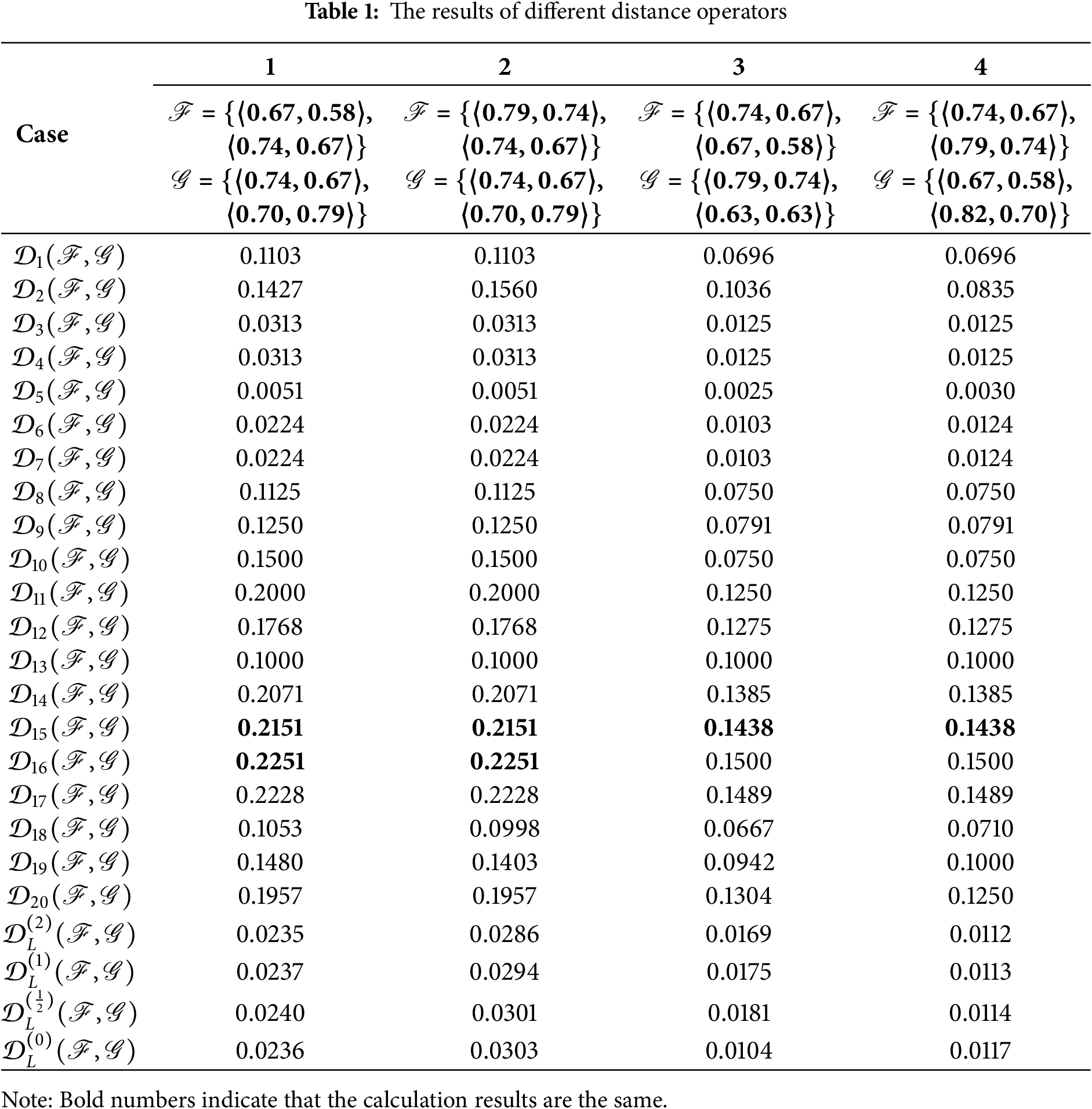
The existing operators show consistent results in several cases, indicating their limited ability to distinguish subtle differences between FFSs. For example,
In contrast, the proposed operators
This section demonstrates the effectiveness of the proposed parametric divergence operator through three representative applications: pattern classification and hierarchical clustering (as typical machine learning tasks), and multiattribute decision-making (as an intelligent decision-making task).
Across the three applications, we aim to establish feasibility, interpretability, and breadth of applicability. Application 1 shows that our operator can be used for pattern recognition with results consistent with most methods. Applications 2 and 3 extend to hierarchical clustering of vehicle buyers and MADM of blockchain platforms selection, respectively, illustrating that the operator integrates well with both machine learning and decision analytics and yields actionable insights.
Let
Step 1: Compute the divergence operator between each reference pattern
Step 2: Determine the minimum divergence value through comparative analysis:
Step 3: Find the classification result of
Step 4: Quantify the discriminative capability using the degree of confidence (
where
Application 1: This application involves a pattern classification task for classifying building materials into four predefined classes using ten attributes [61]. The task is to assign an unknown building material, denoted as
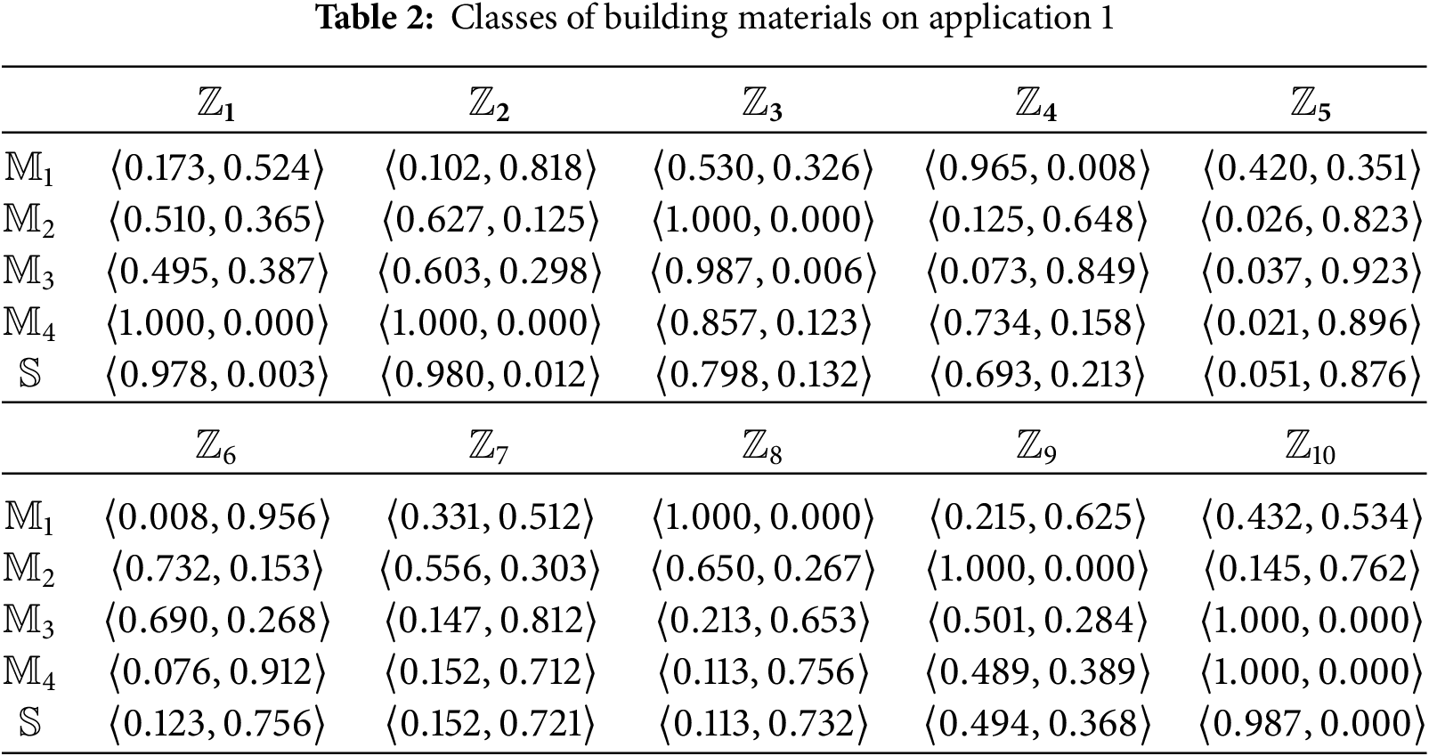
The results are summarized in the Table 3 and Fig. 1. We can learn that across nearly all operators,
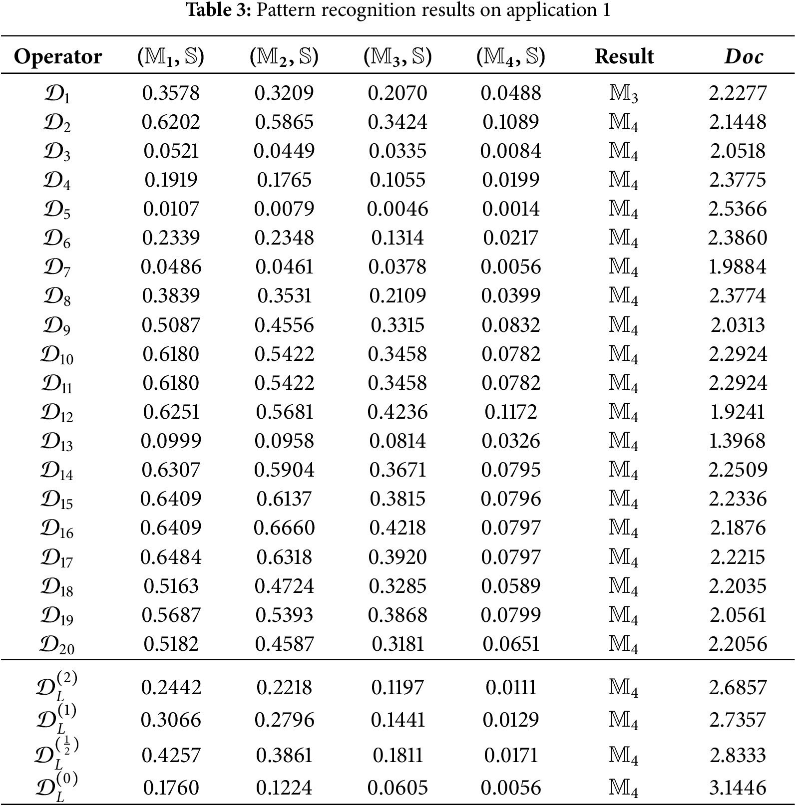
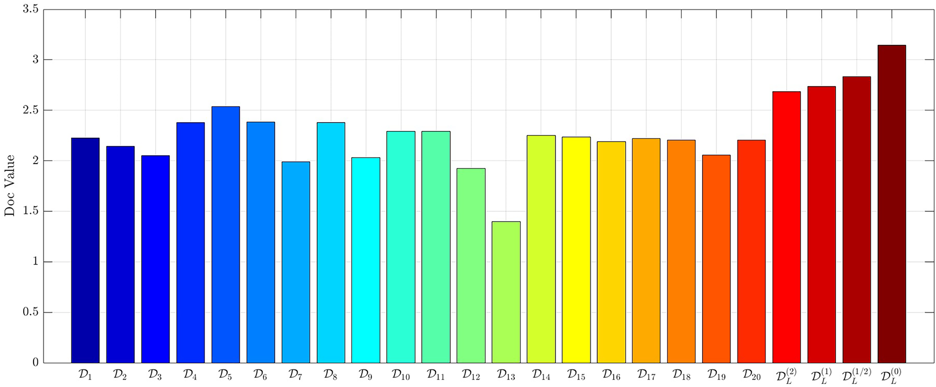
Figure 1:
All operators correctly identified M4 as the classification result, showing consistency across approaches. The proposed operator produced the highest Degree of Confidence (3.1446 versus values between 1.3968 and 2.8333 for other methods), which reflects a clearer separation between the true class and competing alternatives. This suggests that the method may provide more reliable decision support in cases where ambiguity exists.
In this subsection, we use hierarchical clustering to show the performance of the proposed operator. Here we employ the clustering method proposed by [14].
Application 2: In the automotive industry, it is essential to understand consumer preferences to design vehicles that meet different needs and increase customer satisfaction. Automakers can now segment their market based on specific buying patterns and preferences.
We propose a hierarchical clustering method for FFSs to deal with the ambiguity and uncertainty in consumer preferences and behaviors. It will categorize vehicle buyers and provide insights into different buyers. This will help automakers understand the major factors influencing consumer choices and the types of buyers in the market, enabling more targeted product development and marketing strategies. We consider five vehicle buyer types (
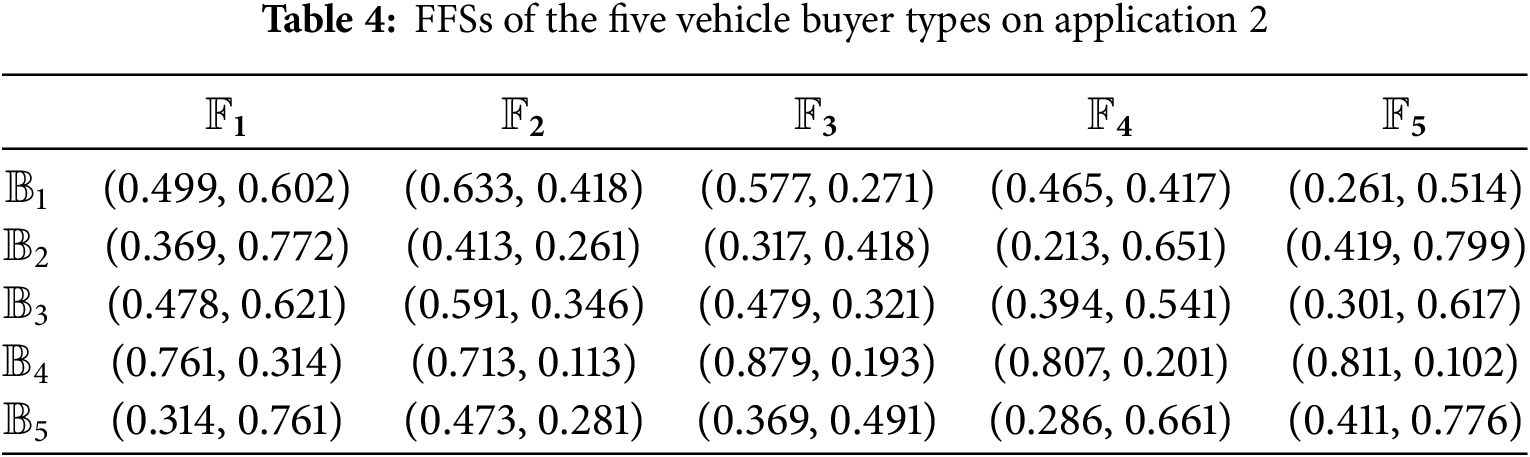
Step 1: Establish the divergence matrix
where
Step 2: Calculate
Then
until
It is clear that
It is evident that
Step 3: Compute the
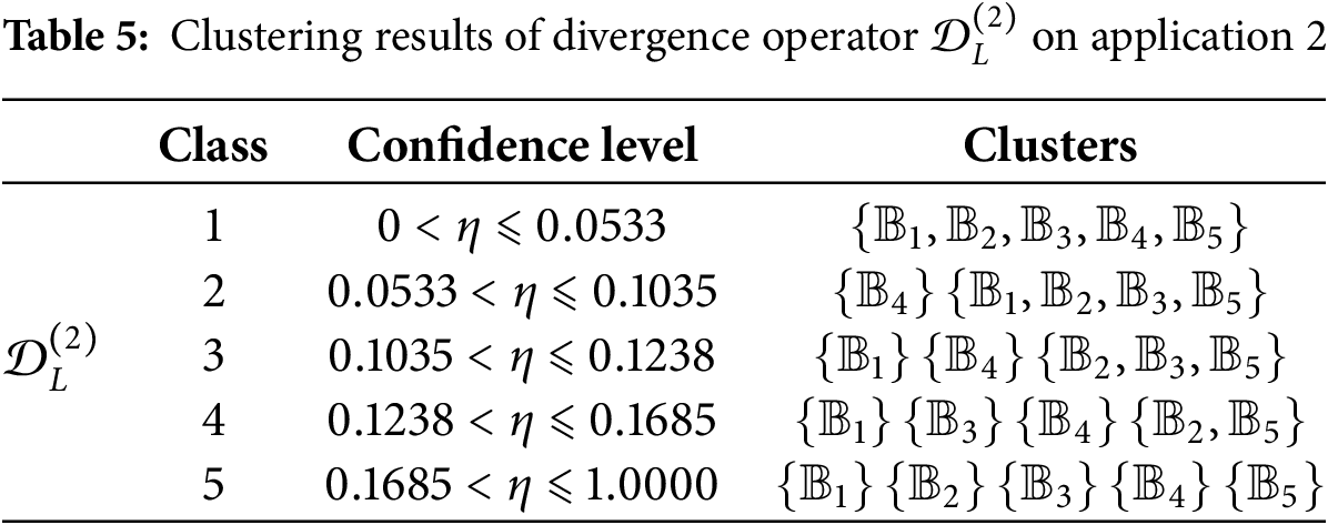
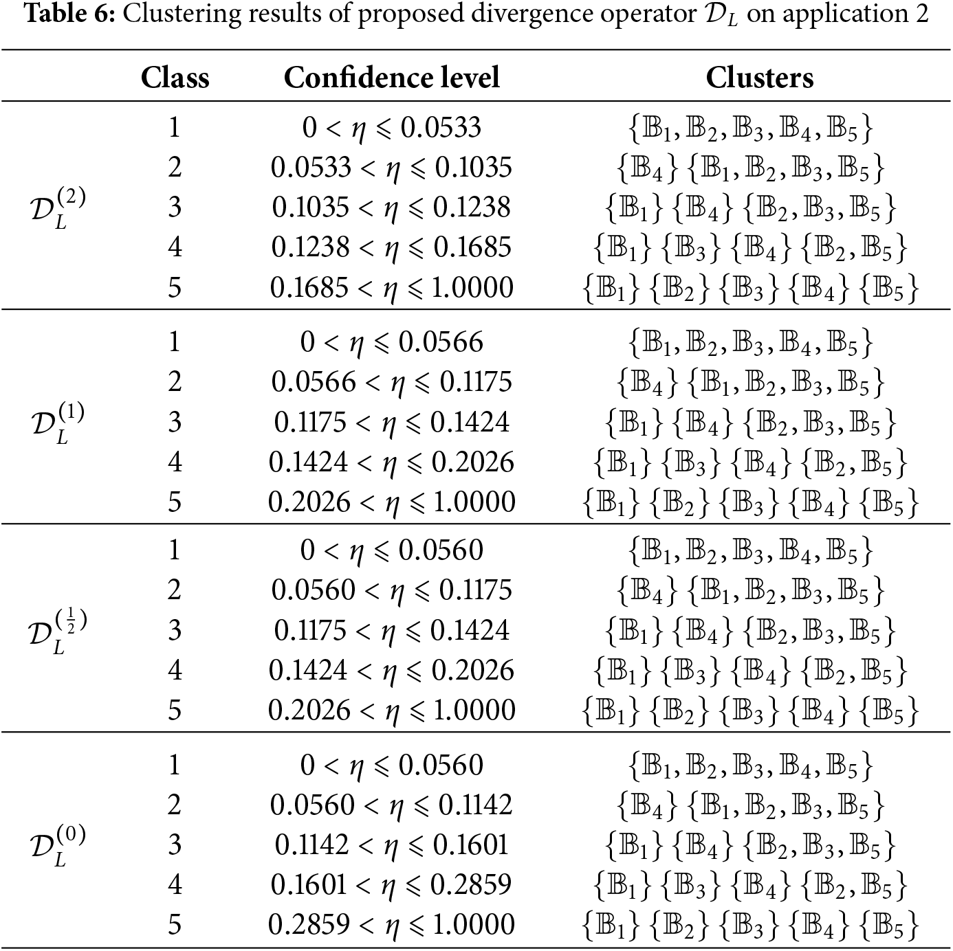
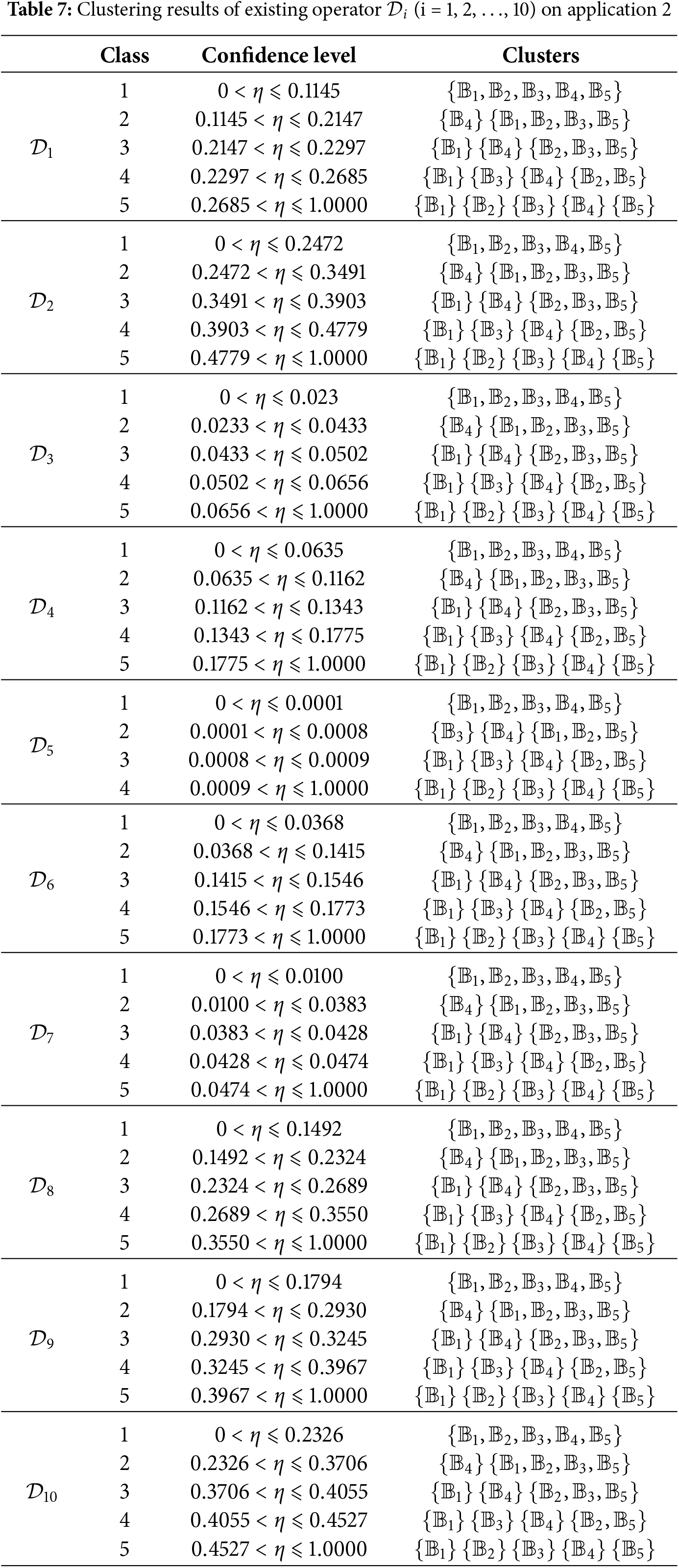
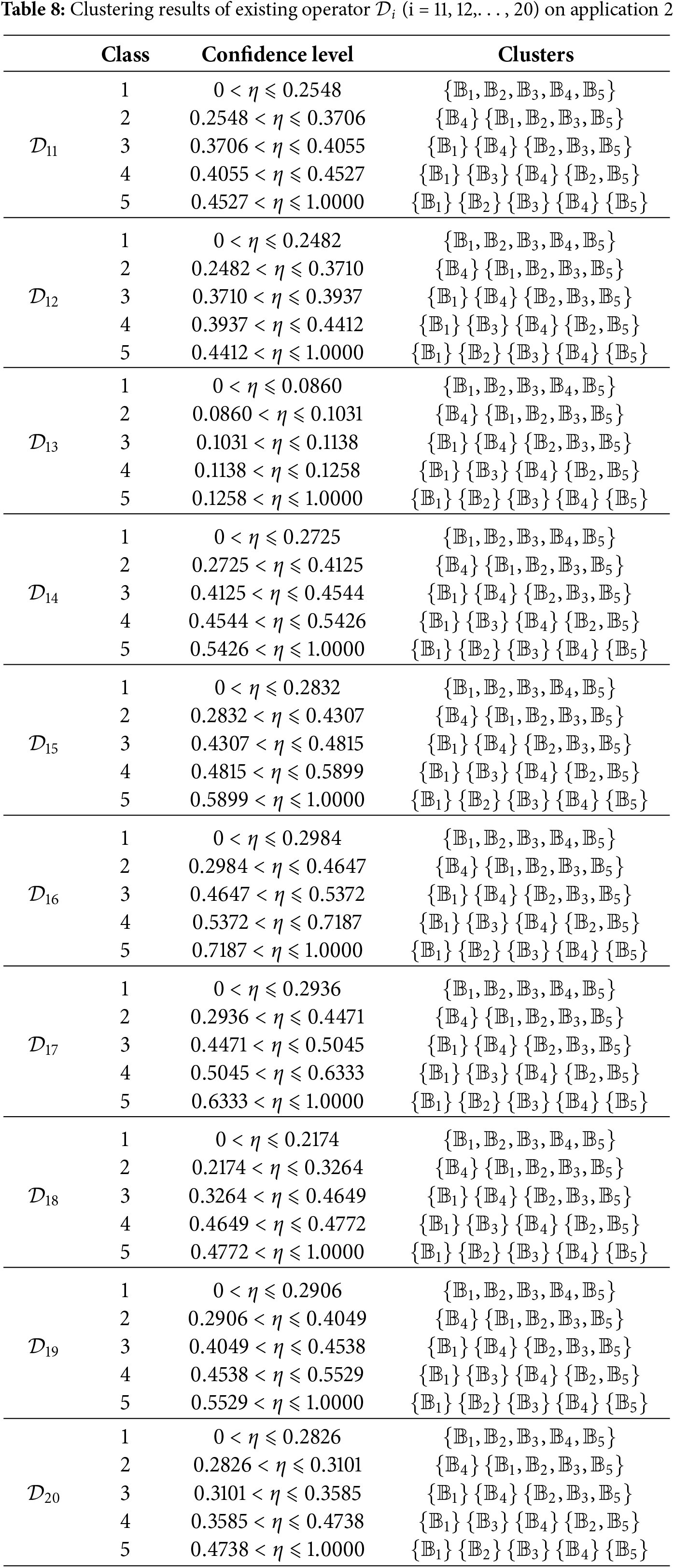
Result Analysis: The clustering results provide automakers with a nuanced understanding of the vehicle buyer market. By identifying the critical factors that influence buyer decisions, manufacturers can tailor their product development and marketing strategies to better meet the specific needs of each buyer segment. For example, targeted marketing campaigns can be designed to appeal to
Significance of Clustering: The proposed operator produces a clustering structure that is both interpretable and actionable for segmenting vehicle buyers. Qualitatively, the early separation of
4.3 Multiattribute Decision Making
• Construct the decision matrix.
Step 1: Given a set of
where
• Compute the criteria weights using proposed divergence operator.
Step 2: It is assumed that each criterion has a different level of importance and that these weights are independent. Let
• Calculate the alternative rankings using AROMAN model.
Step 3: Construct score decision matrix
Step 4: We first use linear normalization to standardize the matrix.
Step 5: Then, we use vector normalization to standardize the matrix.
Step 6: The two normalized matrices are then combined to obtain an aggregated normalization matrix.
where
Step 7: The aggregated normalization matrix is multiplied by the criterion weights to produce a weighted decision matrix.
• Step 8: The benefit attributes are summed using (45), and the cost attributes are summed using (46) to get the normalized weighted values:
Step 9: The performance score for each alternative is calculated by integrating the benefit and cost components.
Here,
4.3.2 Application on Blockchain Platforms Selection
Application 3: In recent years, blockchain technology has emerged as a transformative force in industries such as finance, supply chain, healthcare, and digital identity [62]. As organisations consider adopting blockchain into their operations, selecting the most appropriate platform becomes a critical decision. Given the variety of blockchain platforms available—each with different strengths, trade-offs, and technical specifications—a structured MADM approach is required to ensure an optimal choice that meets strategic objectives.
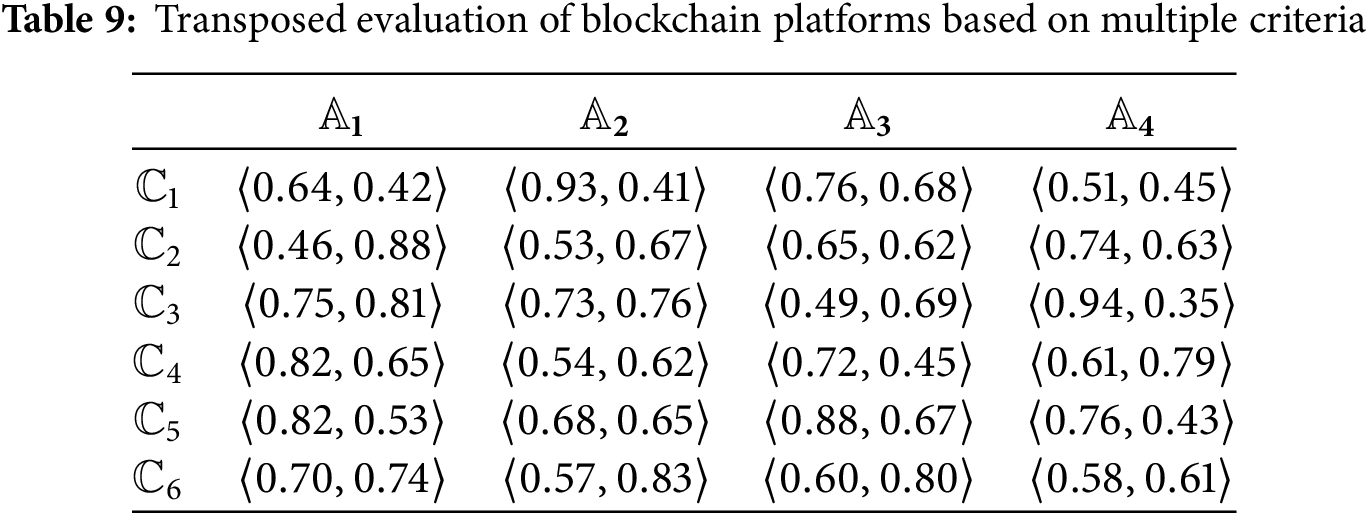
A technology consultancy has been tasked with recommending the most suitable blockchain platform for a consortium of companies that aims to adopt a decentralized application (dApp) for secure, transparent data sharing. The decision involves evaluating four prominent blockchain platforms based on six key criteria.
Blockchain Platforms:
•
•
•
•
Criteria for Evaluation:
• Scalability (Benefit)—The platform’s ability to handle increasing numbers of transactions without performance degradation.
• Operational Expense (Cost)—The total cost of deploying and maintaining applications on the platform.
• Security (Benefit)—The robustness of the platform’s security features, including consensus mechanisms and protection against attacks.
• Interoperability (Benefit)—The ease with which the platform can interact with other blockchain networks and systems.
• Development Maturity (Benefit)—The availability of developer tools, community support, and documentation.
• Governance Complexity (Cost)—The level of difficulty and friction involved in participating in or influencing platform governance decisions.
The consultancy will use a multiattribute decision-making method to rank these platforms and provide a data-driven recommendation.
Our proposed MADM model results are shown in the following part.
Step 1: Construct the blockchain platforms decision matrix
Step 2: The divergence operator
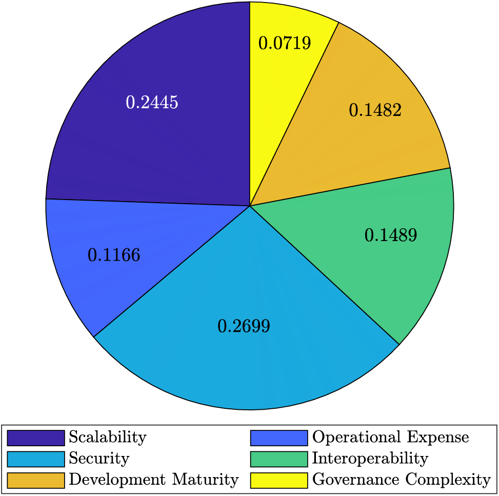
Figure 2: The weight of each attribute
Step 3: The score decision matrix

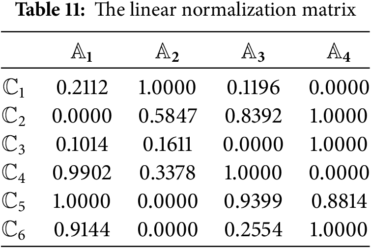
Step 4: Calculate the linear normalization matrix using (41), shown in Table 11.
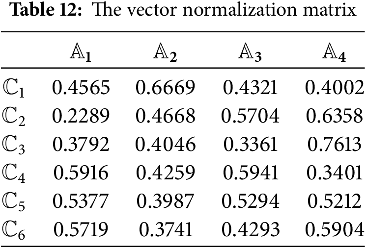
Step 5: Calculate the vector normalization matrix using (42), shown in Table 12.
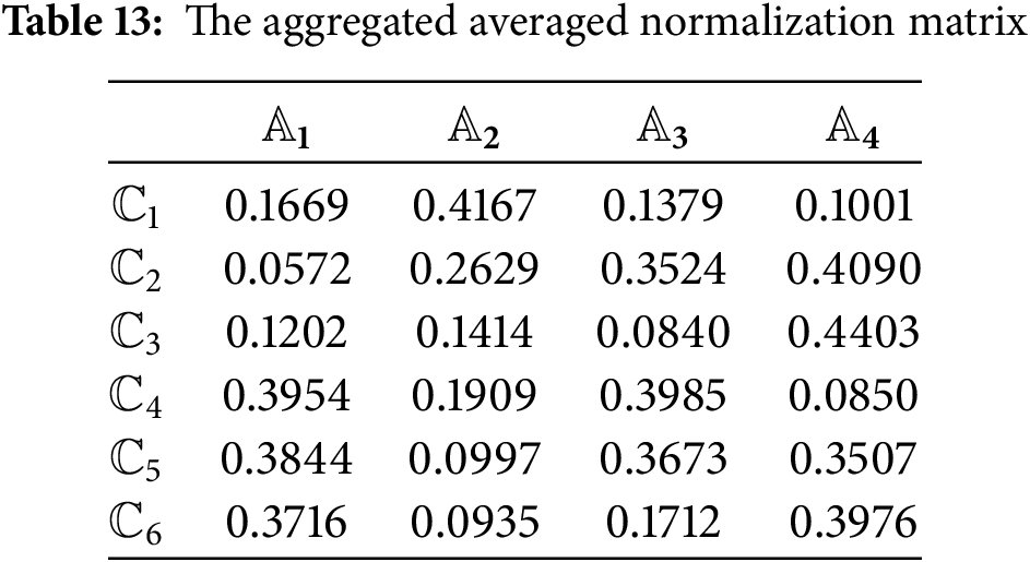
Step 6: Through (43), the aggregated averaged normalization matrix is obtained and displayed in Table 13.
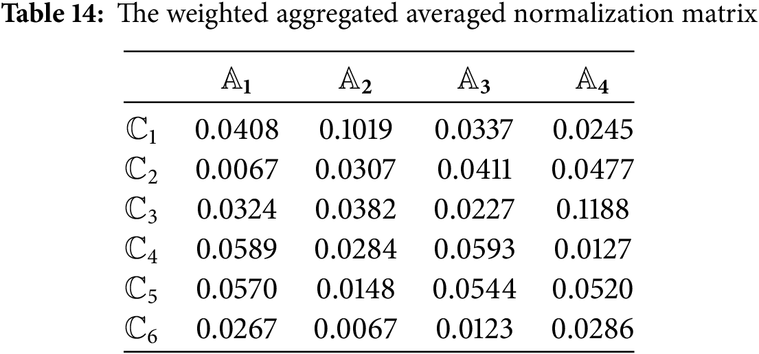
Step 7: Using (44), the weighted aggregated averaged normalization matrix is obtained and displayed in Table 14.
Step 8: The normalized weighted values are computed as:
Step 9: The final ranking of alternatives are shown as:
To evaluate the robustness and validity of the proposed model, a comparative analysis was conducted against several existing decision-making approaches, including the FFS-TOPSIS model [20,44], the FFS-VIKOR method [63]. In the TOPSIS model, a higher final score indicates better performance of the alternatives. In contrast, the VIKOR model follows an opposite convention, where a lower score signifies a more favorable alternative.
The comparative analysis is shown in Table 15 and Fig. 3. The FFS-TOPSIS and the FFS-VIKOR model used the Euclidean distance to determine weight based on (39)
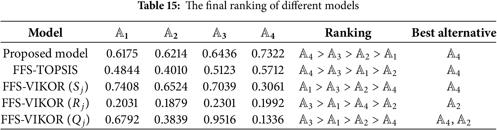
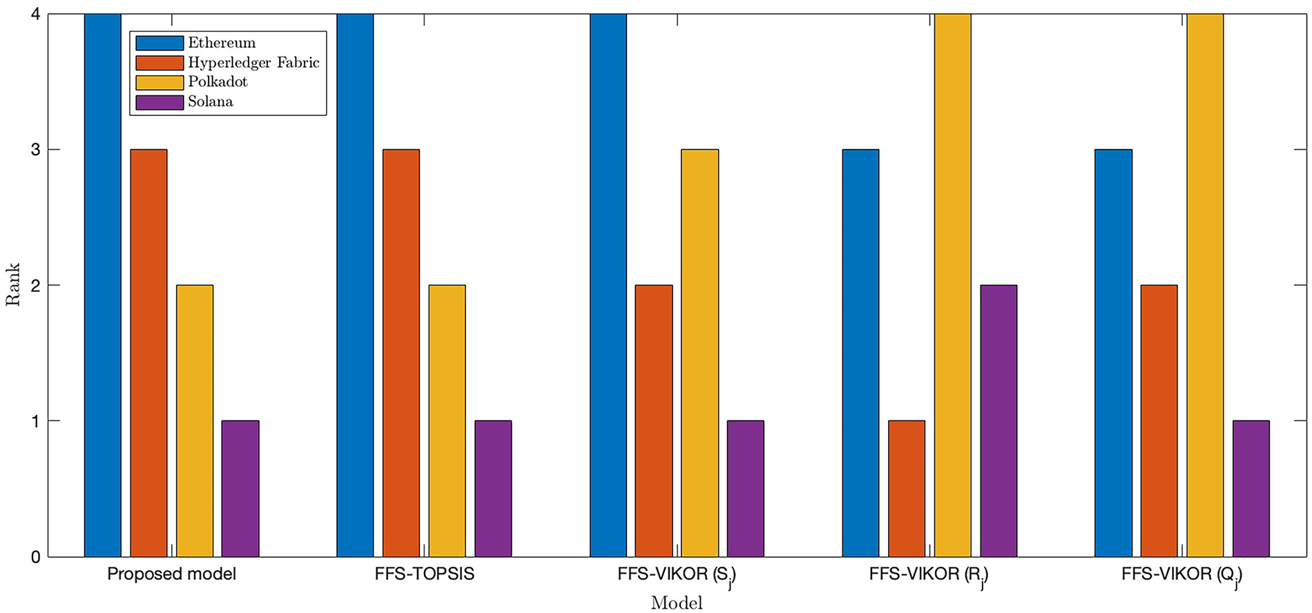
Figure 3: The result of the comparative analysis
To evaluate the stability of the proposed model, this section conducts a sensitivity analysis on three parameters:
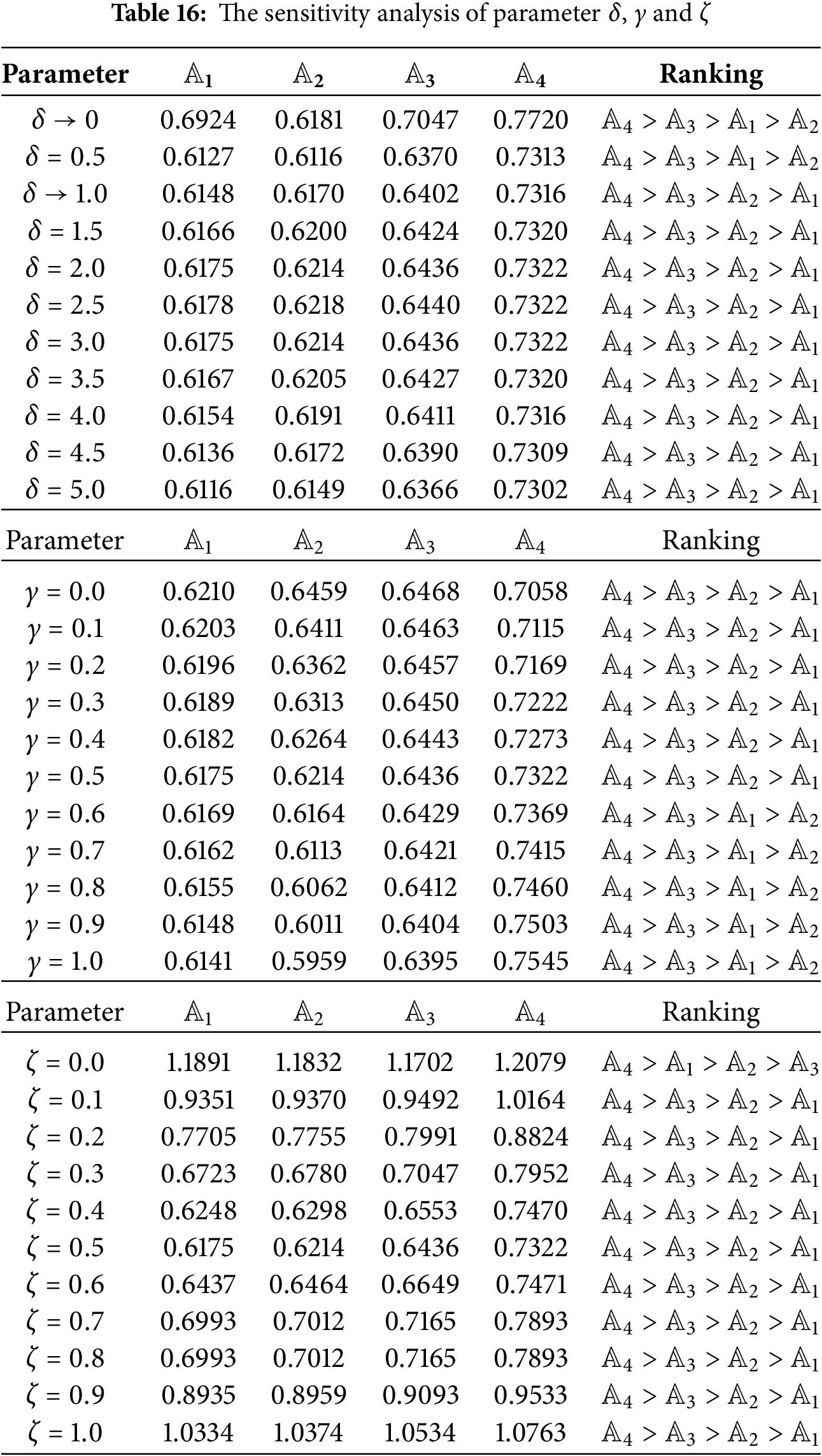
In all three cases, while the utility scores of alternatives show sensitivity to parameter variations, the ranking results remain largely stable. Notably, alternative
This paper introduced a unified Fermatean fuzzy parametric divergence operator that fully accounts for membership, non-membership, and hesitation degrees, addressing key shortcomings in existing divergence operators for FFSs. The proposed operator satisfies fundamental mathematical properties, including non-negativity, non-degeneracy, and symmetry. It also generalizes several well-known divergence operators such as Jensen-Shannon, Hellinger,
Despite the promising outcomes, some limitations should be acknowledged. First, the current divergence operator is defined for precise FFSs, which limits its direct applicability to more complex environments such as interval-valued, complex, or hesitant FFSs. Second, the divergence operator has not yet been integrated into learning-based frameworks, making it less adaptive in dynamic or data-driven decision contexts. Future research will focus on several directions to overcome these limitations. These include generalizing the operator to interval-valued, complex, or hesitant FFSs and embedding the divergence operator within machine learning models such as fuzzy neural networks. Such extensions aim to enhance both the theoretical flexibility and practical utility of the proposed operator in increasingly complex and large-scale decision-making environments.
Acknowledgement: None.
Funding Statement: None.
Author Contributions: Conceptualization, Zhe Liu; methodology, Zhe Liu; validation, Sijia Zhu, Wulfran Fendzi Mbasso, and Himanshu Dhumras; formal analysis, Sijia Zhu, Yulong Huang, and Tapan Senapati; investigation, Zhe Liu, Xiangyu Li, and Wulfran Fendzi Mbasso; visualization, Xiangyu Li and Tapan Senapati; writing—original draft preparation, Sijia Zhu, Xiangyu Li, Wulfran Fendzi Mbasso, and Himanshu Dhumras; writing—review and editing, Zhe Liu, Yulong Huang, Tapan Senapati, and Mehdi Hosseinzadeh; supervision, Yulong Huang, and Mehdi Hosseinzadeh. All authors reviewed the results and approved the final version of the manuscript.
Availability of Data and Materials: All data generated or analyzed during this work are included in this paper. No external datasets were used or deposited in public repositories.
Ethics Approval: Not applicable.
Conflicts of Interest: The authors declare no conflicts of interest to report regarding the present study.
References
1. Gligorić Z, Gligorić M, Miljanović I, Lutovac S, Milutinović A. Assessing criteria weights by the symmetry point of criterion (novel spc method)–application in the efficiency evaluation of the mineral deposit multi-criteria partitioning algorithm. Comput Model Eng Sci. 2023;136(1):955–79. doi:10.32604/cmes.2023.025021. [Google Scholar] [CrossRef]
2. Abdalla MEM, Uzair A, Ishtiaq A, Tahir M, Kamran M. Algebraic structures and practical implications of interval-valued Fermatean neutrosophic super HyperSoft sets in healthcare. Spec Oper Res. 2025;2(1):199–218. [Google Scholar]
3. Liu Z, Letchmunan S. Enhanced fuzzy clustering for incomplete instance with evidence combination. ACM Trans Knowl Discov Data. 2024;18(3):1–20. doi:10.1145/3638061. [Google Scholar] [CrossRef]
4. Tešić D, Marinković D. Application of fermatean fuzzy weight operators and MCDM model DIBR-DIBR II-NWBM-BM for efficiency-based selection of a complex combat system. J Decis Anal Intell Comput. 2023;3(1):243–56. [Google Scholar]
5. Majd SS, Maleki A, Basirat S, Golkarfard A. Fermatean fuzzy TOPSIS method and its application in ranking business intelligence-based strategies in smart city context. J Oper Intell. 2025;3(1):1–16. [Google Scholar]
6. Gokasar I, Pamucar D, Deveci M, Ding W. A novel rough numbers based extended MACBETH method for the prioritization of the connected autonomous vehicles in real-time traffic management. Expert Syst Appl. 2023;211(1):118445. doi:10.1016/j.eswa.2022.118445. [Google Scholar] [CrossRef]
7. Pamucar D, Deveci M, Gokasar I, Brito-Parada PR, Martínez L. Evaluation of process technologies for sustainable mining using interval rough number based heronian and power averaging functions. Knowl Based Syst. 2024;289(4):111494. doi:10.1016/j.knosys.2024.111494. [Google Scholar] [CrossRef]
8. Qi J, Hu J, Huang H, Peng Y. New customer-oriented design concept evaluation by using improved Z-number-based multi-criteria decision-making method. Adv Eng Inform. 2022;53(2):101683. doi:10.1016/j.aei.2022.101683. [Google Scholar] [CrossRef]
9. Nazari-Shirkouhi S, Tavakoli M, Govindan K, Mousakhani S. A hybrid approach using Z-number DEA model and artificial neural network for resilient supplier selection. Expert Syst Appl. 2023;222(04):119746. doi:10.1016/j.eswa.2023.119746. [Google Scholar] [CrossRef]
10. Lyu S, Liu Z. A belief sharma-mittal divergence with its application in multi-sensor information fusion. Comput Appl Math. 2024;43(1):34. doi:10.1007/s40314-023-02542-0. [Google Scholar] [CrossRef]
11. Liu Z, Huang H, Letchmunan S, Deveci M. Adaptive weighted multi-view evidential clustering with feature preference. Knowl Based Syst. 2024;294(3):111770. doi:10.1016/j.knosys.2024.111770. [Google Scholar] [CrossRef]
12. Singh RR, Zindani D, Maity SR. A novel fuzzy-prospect theory approach for hydrogen fuel cell component supplier selection for automotive industry. Expert Syst Appl. 2024;246(3):123142. doi:10.1016/j.eswa.2024.123142. [Google Scholar] [CrossRef]
13. Rong Y, Yu L, Liu Y, Simic V, Pamucar D, Garg H. A novel failure mode and effect analysis model based on extended interval-valued q-rung orthopair fuzzy approach for risk analysis. Eng Appl Artif Intell. 2024;136(1):108892. doi:10.1016/j.engappai.2024.108892. [Google Scholar] [CrossRef]
14. Liu Z. Fermatean fuzzy similarity measures based on Tanimoto and Sørensen coefficients with applications to pattern classification, medical diagnosis and clustering analysis. Eng Appl Artif Intell. 2024;132(1):107878. doi:10.1016/j.engappai.2024.107878. [Google Scholar] [CrossRef]
15. Zadeh LA. Fuzzy sets. Inf Control. 1965;8(3):338–53. [Google Scholar]
16. Atanassov KT. Intuitionistic fuzzy sets. Fuzzy Sets Syst. 1986;20(1):87–96. doi:10.1016/s0165-0114(86)80034-3. [Google Scholar] [CrossRef]
17. Yager RR. Pythagorean membership grades in multicriteria decision making. IEEE Trans Fuzzy Syst. 2014;22(4):958–65. doi:10.1109/tfuzz.2013.2278989. [Google Scholar] [CrossRef]
18. Ejegwa PA, Feng Y, Tang S, Agbetayo JM, Dai X. New Pythagorean fuzzy-based distance operators and their applications in pattern classification and disease diagnostic analysis. Neural Comput Appl. 2023;35(14):10083–95. doi:10.1007/s00521-022-07679-3. [Google Scholar] [CrossRef]
19. Zulqarnain RM, Ma WX, Siddique I, Ahmad H, Askar S. An intelligent MCGDM model in green suppliers selection using interactional aggregation operators for interval-valued pythagorean fuzzy soft sets. Comput Model Eng Sci. 2024;139(2):1829–62. doi:10.32604/cmes.2023.030687. [Google Scholar] [CrossRef]
20. Senapati T, Yager RR. Fermatean fuzzy sets. J Ambient Intell Humaniz Comput. 2020;11(2):663–74. doi:10.1007/s12652-019-01377-0. [Google Scholar] [CrossRef]
21. Senapati T, Yager RR. Fermatean fuzzy weighted averaging/geometric operators and its application in multi-criteria decision-making methods. Eng Appl Artif Intell. 2019;85(S1):112–21. doi:10.1016/j.engappai.2019.05.012. [Google Scholar] [CrossRef]
22. Kakati P, Senapati T, Moslem S, Pilla F. Fermatean fuzzy archimedean heronian mean-based model for estimating sustainable urban transport solutions. Eng Appl Artif Intell. 2024;127(1):107349. doi:10.1016/j.engappai.2023.107349. [Google Scholar] [CrossRef]
23. Saha A, Dabic-Miletic S, Senapati T, Simic V, Pamucar D, Ala A, et al. Fermatean fuzzy dombi generalized maclaurin symmetric mean operators for prioritizing bulk material handling technologies. Cognit Comput. 2024;16(6):3096–121. doi:10.1007/s12559-024-10323-y. [Google Scholar] [CrossRef]
24. Szmidt E, Kacprzyk J. Distances between intuitionistic fuzzy sets. Fuzzy Sets Syst. 2000;114(3):505–18. doi:10.1016/s0165-0114(98)00244-9. [Google Scholar] [CrossRef]
25. Ejegwa PA. Distance and similarity measures for Pythagorean fuzzy sets. Granul Comput. 2020;5(2):225–38. doi:10.1007/s41066-018-00149-z. [Google Scholar] [CrossRef]
26. Ejegwa PA. Modified Zhang and Xu’s distance measure for Pythagorean fuzzy sets and its application to pattern recognition problems. Neural Comput Appl. 2020;32(14):10199–208. doi:10.1007/s00521-019-04554-6. [Google Scholar] [CrossRef]
27. Grzegorzewski P. Distances between intuitionistic fuzzy sets and/or interval-valued fuzzy sets based on the Hausdorff metric. Fuzzy Sets Syst. 2004;148(2):319–28. doi:10.1016/j.fss.2003.08.005. [Google Scholar] [CrossRef]
28. Yang Y, Chiclana F. Consistency of 2D and 3D distances of intuitionistic fuzzy sets. Expert Syst Appl. 2012;39(10):8665–70. doi:10.1016/j.eswa.2012.01.199. [Google Scholar] [CrossRef]
29. Xiao F, Ding W. Divergence measure of Pythagorean fuzzy sets and its application in medical diagnosis. Applied Soft Comput. 2019;79(2):254–67. doi:10.1016/j.asoc.2019.03.043. [Google Scholar] [CrossRef]
30. Wu X, Zhu Z, Chen G, Pedrycz W, Liu L, Aggarwal M. Generalized TODIM method based on symmetric intuitionistic fuzzy Jensen-Shannon divergence. Expert Syst Appl. 2024;237(11):121554. doi:10.1016/j.eswa.2023.121554. [Google Scholar] [CrossRef]
31. Wu X, Zhu Z, Chen SM. Strict intuitionistic fuzzy distance/similarity measures based on Jensen-Shannon divergence. Inf Sci. 2024;661(6):120144. doi:10.1016/j.ins.2024.120144. [Google Scholar] [CrossRef]
32. Li X, Liu Z, Han X, Liu N, Yuan W. An intuitionistic fuzzy version of hellinger distance measure and its application to decision-making process. Symmetry. 2023;15(2):500. doi:10.3390/sym15020500. [Google Scholar] [CrossRef]
33. Liu Z. Hellinger distance measures on pythagorean fuzzy environment via their applications. Int J Knowl-Based Intell Eng Syst. 2024;28(2):211–29. doi:10.3233/kes-230150. [Google Scholar] [CrossRef]
34. Ye J. Cosine similarity measures for intuitionistic fuzzy sets and their applications. Math Comput Model. 2011;53(1–2):91–7. doi:10.1016/j.mcm.2010.07.022. [Google Scholar] [CrossRef]
35. Zhang Q, Hu J, Feng J, Liu A, Li Y. New similarity measures of Pythagorean fuzzy sets and their applications. IEEE Access. 2019;7:138192–202. doi:10.1109/access.2019.2942766. [Google Scholar] [CrossRef]
36. Hwang CM, Yang MS, Hung WL. New similarity measures of intuitionistic fuzzy sets based on the Jaccard index with its application to clustering. Int J Intell Syst. 2018;33(8):1672–88. doi:10.1002/int.21990. [Google Scholar] [CrossRef]
37. Hussain Z, Alam S, Hussain R, ur Rahman S. New similarity measure of Pythagorean fuzzy sets based on the Jaccard index with its application to clustering. Ain Shams Eng J. 2024;15(1):102294. doi:10.1016/j.asej.2023.102294. [Google Scholar] [CrossRef]
38. Tang Y, Wen L, Wei G. Approaches to multiple attribute group decision making based on the generalized Dice similarity measures with intuitionistic fuzzy information. Int J Knowl-Based Intell Eng Syst. 2017;21(2):85–95. doi:10.3233/kes-170354. [Google Scholar] [CrossRef]
39. Patel A, Jana S, Mahanta J. Intuitionistic fuzzy EM-SWARA-TOPSIS approach based on new distance measure to assess the medical waste treatment techniques. Appl Soft Comput. 2023;144(3):110521. doi:10.1016/j.asoc.2023.110521. [Google Scholar] [CrossRef]
40. Kumar R, Kumar S. An extended combined compromise solution framework based on novel intuitionistic fuzzy distance measure and score function with applications in sustainable biomass crop selection. Expert Syst Appl. 2024;239(10):122345. doi:10.1016/j.eswa.2023.122345. [Google Scholar] [CrossRef]
41. Sun G, Wang M. Pythagorean fuzzy information processing based on centroid distance measure and its applications. Expert Syst Appl. 2024;236(4):121295. doi:10.1016/j.eswa.2023.121295. [Google Scholar] [CrossRef]
42. Onyeke IC, Ejegwa PA. Modified Senapati and Yager’s Fermatean fuzzy distance and its application in students’course placement in tertiary institution. In: Real life applications of multiple criteria decision making techniques in fuzzy domain. Cham, Switzerland: Springer; 2022. p. 237–53 doi: 10.1007/978-981-19-4929-6_11. [Google Scholar] [CrossRef]
43. Sahoo L. Similarity measures for Fermatean fuzzy sets and its applications in group decision-making. Decis Sci Letters. 2022;11(2):167–80. [Google Scholar]
44. Kirişci M. New cosine similarity and distance measures for Fermatean fuzzy sets and TOPSIS approach. Knowl Inf Syst. 2023;65(2):855–68. doi:10.1007/s10115-022-01776-4. [Google Scholar] [PubMed] [CrossRef]
45. Liu Z, Huang H. Comment on “new cosine similarity and distance measures for fermatean fuzzy sets and topsis approach”. Knowl Inf Syst. 2023;65(12):5151–7. doi:10.1007/s10115-023-01926-2. [Google Scholar] [CrossRef]
46. Deng Z, Wang J. New distance measure for Fermatean fuzzy sets and its application. Int J Intell Syst. 2022;37(3):1903–30. doi:10.1002/int.22760. [Google Scholar] [CrossRef]
47. Ganie AH. Multicriteria decision-making based on distance measures and knowledge measures of Fermatean fuzzy sets. Granul Comput. 2022;7(4):979–98. doi:10.1007/s41066-021-00309-8. [Google Scholar] [PubMed] [CrossRef]
48. Behzadian M, Otaghsara SK, Yazdani M, Ignatius J. A state-of the-art survey of TOPSIS applications. Expert Syst Appl. 2012;39(17):13051–69. doi:10.1016/j.eswa.2012.05.056. [Google Scholar] [CrossRef]
49. Gul M, Celik E, Aydin N, Gumus AT, Guneri AF. A state of the art literature review of VIKOR and its fuzzy extensions on applications. Appl Soft Comput. 2016;46:60–89. doi:10.1016/j.asoc.2016.04.040. [Google Scholar] [CrossRef]
50. Torkayesh AE, Deveci M, Karagoz S, Antucheviciene J. A state-of-the-art survey of evaluation based on distance from average solution (EDASdevelopments and applications. Expert Syst Appl. 2023;221(1):119724. doi:10.1016/j.eswa.2023.119724. [Google Scholar] [CrossRef]
51. Chang TH. Fuzzy VIKOR method: a case study of the hospital service evaluation in Taiwan. Inf Sci. 2014;271(3):196–212. doi:10.1016/j.ins.2014.02.118. [Google Scholar] [CrossRef]
52. Ghorabaee MK, Amiri M, Zavadskas EK, Hooshmand R, Antuchevičienė J. Fuzzy extension of the CODAS method for multi-criteria market segment evaluation. J Bus Econ Manag. 2017;18(1):1–19. doi:10.3846/16111699.2016.1278559. [Google Scholar] [CrossRef]
53. Salih MM, Zaidan B, Zaidan A, Ahmed MA. Survey on fuzzy TOPSIS state-of-the-art between 2007 and 2017. Comput Operat Res. 2019;104:207–27. [Google Scholar]
54. Ogundoyin SO, Kamil IA. An integrated fuzzy-BWM, fuzzy-LBWA and V-fuzzy-CoCoSo-LD model for gateway selection in fog-bolstered Internet of Things. Appl Soft Comput. 2023;143(5):110393. doi:10.1016/j.asoc.2023.110393. [Google Scholar] [CrossRef]
55. Bošković S, Švadlenka L, Jovčić S, Dobrodolac M, Simić V, Bacanin N. An alternative ranking order method accounting for two-step normalization (AROMAN)—a case study of the electric vehicle selection problem. IEEE Access. 2023;11(3):39496–507. doi:10.1109/access.2023.3265818. [Google Scholar] [CrossRef]
56. Nikolić I, Milutinović J, Božanić D, Dobrodolac M. Using an interval type-2 fuzzy AROMAN decision-making method to improve the sustainability of the postal network in rural areas. Mathematics. 2023;11(14):3105. doi:10.3390/math11143105. [Google Scholar] [CrossRef]
57. Kara K, Yalçın GC, Acar AZ, Simic V, Konya S, Pamucar D. The MEREC-AROMAN method for determining sustainable competitiveness levels: a case study for Turkey. Socioecon Plann Sci. 2024;91(48):101762. doi:10.1016/j.seps.2023.101762. [Google Scholar] [CrossRef]
58. Deveci M, Varouchakis EA, Brito-Parada PR, Mishra AR, Rani P, Bolgkoranou M, et al. Evaluation of risks impeding sustainable mining using Fermatean fuzzy score function based SWARA method. Appl Soft Comput. 2023;139(1):110220. doi:10.1016/j.asoc.2023.110220. [Google Scholar] [CrossRef]
59. Mishra AR, Rani P, Saha A, Senapati T, Hezam IM, Yager RR. Fermatean fuzzy copula aggregation operators and similarity measures-based complex proportional assessment approach for renewable energy source selection. Complex Intell Syst. 2022;8(6):5223–48. doi:10.1007/s40747-022-00743-4. [Google Scholar] [PubMed] [CrossRef]
60. Zhu S, Liu Z, Ulutagay G, Deveci M, Pamučar D. Novel α-divergence measures on picture fuzzy sets and interval-valued picture fuzzy sets with diverse applications. Eng Appl Artif Intell. 2024;136(12):109041. doi:10.1016/j.engappai.2024.109041. [Google Scholar] [CrossRef]
61. Bozyiugit MC, Olgun M, Ünver M, Söylemez D. Parametric picture fuzzy cross-entropy measures based on d-Choquet integral for building material recognition. Appl Soft Comput. 2024;166(3):112167. doi:10.1016/j.asoc.2024.112167. [Google Scholar] [CrossRef]
62. Nanayakkara S, Rodrigo M, Perera S, Weerasuriya GT, Hijazi AA. A methodology for selection of a Blockchain platform to develop an enterprise system. J Ind Inf Integr. 2021;23(04):100215. doi:10.1016/j.jii.2021.100215. [Google Scholar] [CrossRef]
63. Gül S. Fermatean fuzzy set extensions of SAW, ARAS, and VIKOR with applications in COVID-19 testing laboratory selection problem. Expert Syst. 2021;38(8):e12769. doi:10.1111/exsy.12769. [Google Scholar] [PubMed] [CrossRef]
Cite This Article
 Copyright © 2025 The Author(s). Published by Tech Science Press.
This work is licensed under a Creative Commons Attribution 4.0 International License , which permits unrestricted use, distribution, and reproduction in any medium, provided the original work is properly cited.
 Downloads
 Citation Tools