Random Eigenvibrations of Internally Supported Plates by the Boundary Element Method

1  Introduction

The main aim of this work is the study of an application of the Boundary Element Method (BEM) to the natural thin (Kirchhoff) plate vibration problem by the probabilistic approach. The foundations of the Boundary Element Method date back to the 1950s [1], with the works of Kupradze [2] and Michlin [3] being most often cited. A series of works presented by Jaswon and Symm have shown the usefulness of formulating the elastic problem in terms of a potential [4,5]. The fundamental works on the analysis of plate bending in terms of boundary integral equations were presented by Stern [6], Altiero and Sikarskie [7], and Bèzine with Gamby [8]. A modified theory of thin plate bending in terms of the BEM has been presented by El-Zafrany et al. [9]. The general concept of BEM was presented by Burczyński [10]. Katsikadelis [11] proposed a BEM solution for dynamic problems of plates. Katsikadelis et al. [12] employed the BEM approach for the static and dynamic analysis of plates with internal supports. In later years, several works related to plate dynamics were published, including those by Beskos [13], Katsikadelis and Sapountzakis [14], Katsikadelis and Yotis [15], and Wen et al. [16]. Notably, the work by [14] analyzes the dynamics of plates with variable stiffness. The exciting work presented by Katsikadelis with Babouskos [17] is recommended, where they used the so-called Analog Equation Method (AEM) coupled with the Domain Boundary Element Method (DBEM) to investigate a flutter instability of plates.

According to the classical Kirchhoff-Love plate theory, an unavoidable inconvenience is the occurrence of concentrated forces at the corner points. This results from the need to reconcile the number of unknowns at the boundary with the order of the differential equation of the plate. This inconvenience can be easily eliminated by assuming that the boundary elements in the immediate vicinity of the corner can act as corner forces distributed over a specific section of the edge. This concept for statics, dynamics, fluid-plate interaction, and initial stability of plates with various shapes, boundary conditions, and support conditions, was performed by Guminiak [18].

A specific formulation of the BEM has also been used in solutions to various boundary value problems with uncertainties, random fields, or stochastic processes. The stochastic perturbation technique in terms of the BEM has been proposed by Kamiński [19], and Wang and Guo applied the same method for piezoelectric problems [20]. Guminiak and Kamiński applied a semi-analytical probabilistic approach to natural vibrations of plates fully immersed in fluid [21]. Karakostas and Manolis investigated the dynamic response of tunnels in stochastic soils by the BEM [22]. Zhang et al. applied a stochastic perturbation technique to the numerical analysis of a structure-acoustic system [23]. Su et al. performed a reliability analysis of plane elasticity problems and Reissner plates by stochastic spline fictitious BEM [24,25]. This probabilistic conception has been extended to the study of linear-elastic cracked structures [26]. In the next work, authored by Su et al., the probabilistic approach to vibrations of elastic plane problems is presented [27].

On the other hand, Chowdhury and Gao investigated probabilistic fracture mechanics in terms of the scaled boundary finite element method [28,29], where the Monte Carlo simulation (MCS) approach was applied [28]. The scaled boundary finite elements have been applied by Do et al., where the domain has been randomly determined [30]. Kamiński applied the generalized iterative stochastic perturbation technique (SPT) coupled with finite element analysis to determine the probabilistic moments of the structural response [31]. Generally the values defining the material as well as the geometry and external loading of a structure may be of random nature. Schiantella et al. presented the influence of geometrical uncertainties on the failure load estimation of lattice structures [32]. Huang and Beer estimated the probability distribution for dynamic and extreme responses of linear elastic structures under quasi-stationary harmonizable loads [33]. Uncertainty quantification for viscoelastic composite materials using time-separated stochastic mechanics was investigated by Geisler and Junker [34]. On the other hand Huang et al. presented nonlinear random vibrations of a slender pier surrounded by liquid and loaded seismically [35]. This paper presents the concept of natural vibrations of plates supported at their boundaries and within their own domain, using the Boundary Element Method, with simplified and modified boundary conditions, in a random approach. The random variables will be the material characteristics, such as Young’s modulus, Poisson’s ratio, and the plate thickness. The obtained solution, in the form of the expected value, coefficient of variation, skewness, and kurtosis, will be determined within the range of the coefficient of variation of the design parameter.

2  Structural Eigenvibrations of Kirchhoff-Love Plate with Internal Constraints

The problem of free vibrations of a plate is considered. A discrete mass distribution inside the plate domain is assumed. At each of the internal collocation points associated with a single concentrated mass mi, the following quantities are introduced: wi, acceleration w¨i, and inertia force Bi, where i denotes the point inside the plate domain where a single lumped mass is located. Column supports are modeled as a rectangular subdomain with a single, centrally located collocation point, where the column reaction is distributed uniformly over the surface of this domain. Internal continuous linear supports are introduced similarly and are modeled as segments with a single central collocation point. The fundamental solution (Green’s function), e.g., Refs. [9,14] for statics, is used to solve the problem w∗(y,x)=(1/(8πD))r2ln⁡(r) and r=|y−x|, where x is the source point and y is a field point, D=Eh3/[12(1−v2)] is the plate stiffness, h is a plate thickness, E and v are the Young’s modulus and the Poisson’s ratio, respectively.

For harmonic vibrations, the vertical displacement of the i-th lumped mass, the acceleration, and the inertia force assigned to it can be expressed:

wi(t)=W~isin⁡ωt,w¨i(t)=−ω2W~isin⁡ωt,Bi(t)=B~isin⁡ωt,(1)

where ω is a natural frequency of the elastic plate under consideration, W~i and B~i=−ω2W~i are the amplitudes of displacement and inertial forces associated with the i-th lumped mass.

The governing boundary and domain integral equations have the character of amplitude equations, and they are derived using Betti’s theorem:

c(x)w(x)+∫Γ[Tn∗(y,x)w(y)−Mns∗(y,x)dw(y)ds−Mn∗(y,x)φn(y)]dΓ(y)=∫Γ[T~n(y)w∗(y,x)−Mn(y)φn∗(y,x)]dΓ(y)+∑i=1Nω2miW~iw∗(y,i)−∫ΩjRjw∗(j,x)dΩj−∫ΓkTkw∗(k,x)dΓk,(2)

c(x)φ¯n(x)+∫Γ[T¯n∗(y,x)w(y)−M¯ns∗(y,x)dw(y)ds−M¯n∗(y,x)φn(y)]dΓ(y)=∫Γ[T~n(y)w¯∗(y,x)−Mn(y)φ¯n∗(y,x)]dΓ(y)+∑i=1Nω2miW~iw¯∗(y,i)−∫ΩjRjw¯∗(j,x)dΩj−∫ΓkTkw¯∗(k,x)dΓk,(3)

where Rj and Tk denote reaction in the j-th column and in the k-th element of the whole column and continuous support, respectively, and w(y), φn(y), φs(y) denote the deflection amplitudes and the angles of rotation normal and tangential to the plate edge, respectively, finally T~n(y), Mn(y) denote the amplitudes of the transverse force at the edge (together with the forces at the corners) and the moment normal to the edge of the plate. The quantities marked with an asterisk denote the corresponding fundamental functions, i.e., the fundamental solution w∗ and its derivatives with respect to variables n and s. The coefficient c(x) is equal to 0, 0.5, and 1 in the case when the collocation point is placed outside a plate, directly on a boundary, and inside a plate domain, respectively.

In the above two equations, the terms refer to both column and continuous linear supports; however, in the numerical examples, the types of these supports will appear individually. In Eqs. (2) and (3), the angle of rotation tangential to the free edge of the plate, φs(y)=dw(y)/ds, is not an independent quantity and is expressed by the derivative of the deflection with respect to the tangent coordinate.

Construction of the Set of Algebraic Equations

A plate boundary is divided into a finite number of boundary elements of the constant type. It is a proven and reliable boundary element. Additionally, to simplify the computational procedures, a non-singular approach will be employed, where a single collocation point is located outside the plate domain. This conception is illustrated in Fig. 1.

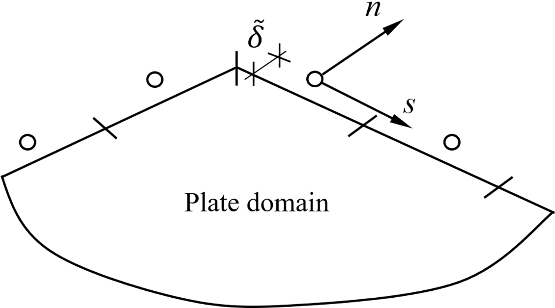
Figure 1: Discretization of a plate boundary using boundary elements of the constant type and a non-singular approach

The construction of a set of algebraic equations requires the calculation of appropriate boundary integrals, integrals along internal linear supports (they are similar to boundary integrals), surface integrals within sub-areas acting as column supports, and the calculation of the values of fundamental functions at points to which concentrated masses are assigned. The straight boundary elements of the constant type are applied. The set of algebraic equations in matrix notation is in the form:

[GBBΔGRBGwBGBS−IGRSGwSGBR   0GRRGwR−λGBwMp       0−λGRwMp−λGwwMp+I]{B~φ~SR~w~}={0000},(4)

where λ=ω2 and B~, φ~S denote vectors of the boundary quantities amplitudes, R~, w~ denote vectors of internal support reactions amplitudes and vertical displacements amplitudes at the internal collocation points coupled with lumped masses. GBB and GBS are the matrices of dimension (2n×2n) and of dimension (2n×S), respectively, grouping boundary integrals (integrals from boundary collocation points over the boundary elements), and they depend on the type of boundary; n is the number of boundary elements of the constant kind, and S is the number of boundary elements along free edges. The GBR is the matrix of dimension (2n×R) collecting integrals from boundary collocation points of the function w∗ over the column sub-domains or integrals along internal linear elements. Further, the GBw is the matrix of dimension (2n×M) collecting values of the fundamental function w∗ in coordinate systems fixed at boundary collocation points, which are established at internal collocation points (M is the number of internal collocation points and n is the number of boundary nodes or elements of the constant type). In general, the following integral relations can be written as follows

(GBB(1,1))e=∫Γeg1(1)dΓe,(GBB(1,2))e=∫Γeg1(2)dΓe,(5)

(GBB(2,1))e=∫Γeg2(1)dΓe,(GBB(2,2))e=∫Γg2(2)dΓe,(6)

where “e” denotes boundary element, “(1)” denotes the first boundary condition coupled with the first fundamental solution w∗(y,x), “(2)” denotes the second boundary condition coupled with the second fundamental solution w¯∗(y,x)=∂w∗(y,x)/∂n wherein the functions g1 and g2 are the corresponding fundamental functions derived from the first and second fundamental solutions, i.e., g1=w∗(y,x), g1=w¯∗(y,x), and dependent on the boundary condition, where for the free edge one should add

(GBS(1,2))e=∫Γeg1(2s)dΓe,(GBS(2,2))e=∫Γeg2(2s)dΓe,(7)

where “s” denotes free boundary and a rotation tangential to it, e.g., g1(2s)g12s=Mns∗(y,x), and g2(2s)=M¯ns∗(y,x),

(GBR(1,1))e=∫Γrg1(1)dΓr,(GBR(2,1))e=∫Γrg2(1)dΓr,(8)

where “r” denotes internal continuous support (internal linear element), and

(GBw(1,1))e=∑n=1N(g1(1))n,(GBw(2,1))e=(g2(1))n,(9)

where “w” denotes an internal collocation point (generally the set of internal collocation points) coupled with a lumped mass (coupled with lumped masses). In the case of column supports, integrals over straight line (8) segments are replaced by integrals over the column surface.

Additionally, a parameter Δ collects the difference operators of the first-order coupling angles of rotations in the tangent direction φs(y), with deflections of suitable three adjacent boundary nodes, only in the case when a plate has a free edge. This angle is expressed as follows

φs(r−1)=1d(−32wr−1+2wr−12wr+1)(10)

φs(r)=12d(wr+1−wr−1)(11)

φs(r+1)=1d(12wr−1−2wr+32wr+1)(12)

Expression (10) is used for an element (collocation point) located at the beginning of a free edge, and expression (11) is used for the elements located inside this edge. Finally, expression (12) is used for the element located last on the free edge. These relationships are illustrated in Fig. 2.

Figure 2: Expression of the angle of rotation in the tangent direction by the deflections of three adjacent nodes. Designations for expressions

In turn, GRB and GRS are matrices of dimensions (R×2n) and (R×S), respectively. They collect boundary integrals of the appropriate fundamental functions from coordinate systems, coupled with internal collocation points that belong to the column or linear supports. Moreover, GRR is the matrix of dimension (R×R) collecting integrals of the function w∗ over the column sub-domains or integrals along internal linear elements from coordinate systems coupled with internal collocation points belonging to the column or linear supports. The GRw is an R×M matrix that collects the values of the fundamental function w∗ established at internal collocation points associated with lumped masses from coordinate systems coupled with internal collocation points belonging to the column or linear supports. Similarly, as above, the following integrals can be written:

(GRB(1,1))r=∫Γeg1(1)dΓe,(GRB(1,2))r=∫Γeg1(2)dΓe,(13)

(GRS(1,1))r=∫Γeg1(2s)dΓe,(14)

(GRR(1,1))r=∫Γrg1(1)dΓr,(15)

(GRw(1,1))r=∑n=1N(g1(1))n.(16)

Additionally, GwB and GwS are matrices of dimensions (M×2n) and (M×S), respectively, collecting boundary integrals of the appropriate fundamental functions from coordinate systems coupled with internal collocation points belonging to lumped masses. In our model, GwR is a matrix of dimension (M×R) that collects integrals of the function w∗ over the column sub-domains or integrals along internal linear elements from coordinate systems coupled with internal collocation points belonging to lumped masses. Furthermore, Gww is the matrix of the dimension (M×M), which includes the values of the fundamental function w∗ calculated at internal collocation points coupled with lumped masses from coordinate systems associated with internal collocation points belonging to lumped masses, and

(GwB(1,1))w=∫Γeg1(1)dΓe,(GwB(1,2))w=∫Γeg1(2)dΓe,(17)

(GwS(1,1))w=∫Γeg1(2s)dΓe,(18)

(GwR(1,1))w=∫Γrg1(1)dΓr,(19)

(Gww(1,1))w=∑n=1N(g1(1))n.(20)

Finally, Mp(M×M) is a plate lumped mass matrix. Graphical interpretation of the above matrices on the example of a plate with column supports is given in Fig. 3. Standard symbols (letters) used previously in works, e.g., [18], related to statics, dynamics, and stability of plates in the BEM approach with a modified (simplified) formulation of boundary conditions were used for explanations.

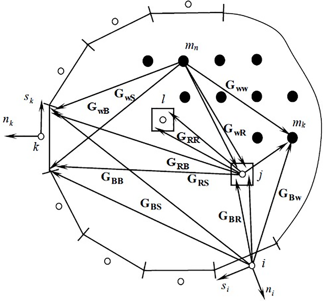
Figure 3: Notation for the discrete Eq. (4) [18]

All boundary integrals are calculated in the coordinate system associated with the ith element (collocation point) from which the integration is performed. They are then transformed to the coordinate system associated with the kth boundary element along which the integration is performed. The same thing happens with integrals inside the domain of the field, i.e., integrals of the fundamental solution w∗ are transformed in an identity manner, integrals of fundamental moments Mn∗,Ms∗, and Mns∗ are transformed as a tensor with valence 2, and finally integrals from fundamental shear forces Tn∗ and Ts∗ are transformed as a vector. The integrals for the basic solution w¯∗=∂w∗/∂n are transformed identically.

Elimination of the amplitudes of the boundary quantities and the matrix Eq. (4) allows us to obtain the standard eigenvalue problem

{A−λ~I}w~=0,(21)

where λ~=1/ω2,

A=(CwBCBB−1CBw−Cww)Mp(22)

and,

CBB=GBB+GBSΔ−GBRGRR−1(GRB+GRSΔ),CBw=GBRGRR(−1)GRw−GBw,CwB=GwB+GwSΔ−GwRGRR−1(GRB+GRSΔ),Cww=GwRGRR−1GRw−Gww(23)

3  Probabilistic Approach to the Boundary Element Method

Initially, the sets of deterministic solutions are needed to carry out further probabilistic analysis. A continuous Gaussian probability distribution, p(x) for all random variables, is assumed, where x is the domain of occurrence of a given phenomenon (design parameter). Due to the continuity of the probability distribution, deterministic results should be transformed to the continuous form. For this purpose, the results are fitted using polynomial curves, where the polynomial coefficients are determined by the Least Squares Method (LSM) or by weighted averages. Each natural frequency can be expressed as follows:

ωi(X)=∑j=0nCijXj.(24)

Next, the fundamental probabilistic characteristics, such as expectations, coefficients of variation, skewness, and kurtosis, are defined, e.g., Ref. [19]:

E[ωi]=∫−∞+∞⁡∑j=1n⁡Cijrjp(x)dx,α(ωi)=|σ(ωi)E[ωi]|,β(ωi)=μ3(ωi)σ3(ωi),κ(ωi)=μ4(ωi)σ4(ωi)−3(25)

Next, let Q be the admissible limit of the given structure, and P the corresponding extreme effort. The satisfactory safety may be measured using the FORM reliability index:

βFORM=E[Q]−E[P]Var(Q−P)=E[ωi]−E[34ωi]σ(ωi−34ωi).(26)

A similar safety measure is defined by the use of probabilistic relative entropy, and calculated due to the Bhattacharyya relative entropy theory as [36]:

H=14(E[Q]−E[P])2σ2(Q)+σ2(P)+12ln⁡(σ2(Q)+σ2(P)2σ(Q)σ(P)).(27)

This measure can be reduced to the previous one:

βH=12H(ωi).(28)

Let X be a random quantity that follows the Gaussian normal distribution with its mean value μ and standard deviation σ, and let a polynomial function be given in the form (usually, the third-degree polynomials adequately describe the response fit curves of the structure):

f=C3X3+C2X2+C1X+C0.(29)

Then the expected value of f can be expressed in a simple way:

E(f)=(μ3+3μσ2)C3+(μ2+σ2)C2+μC1+C0(30)

Similarly, the standard deviation is expressed in the same way:

σ(f)=(9μ4σ2C32+36μ2σ4C32+15σ6C32+12μ3σ2C2C3+24μσ4C2C3+6μ2σ2C1C3+4μ2σ2C22+6σ4C1C3+ 2σ4C22+4σ2C1C2+σ2C12)12.(31)

The above expressions enable a straightforward prediction of the solution in a two-dimensional space defined by the mean value and standard deviation of the selected design parameter. For the fourth-order polynomial fitness function, we obtain much more complicated analytical expressions.

The procedure of fitting polynomial response curves of a structure generally described by the relation (24) can also be performed using the weighted version of the LSM. The number of weights is equal to the number of all deterministic solutions. A symmetrical distribution of weights is also assumed, whereby the mean value of the design parameter is assigned the most significant weight value. Therefore, an odd number of deterministic results is desirable. The sum of the remaining values of the remaining weights is equal to the value of the most significant weight.

Accurate determination of the fitting curves is the most important element of a probabilistic analysis, because too high a degree of the polynomial basis may lead to overestimation of some probabilistic moments and remarkable oscillations of the response curve. On the other hand, a too low degree of this basis usually leads to an underestimation of the mean values of structural response and some discrepancies in the fluctuations of the coefficients of variation.

The Monte Carlo method is based on the law of large numbers, which states that the probability of a correct result (success) increases as the number of trials increases. This means that a large, or ideally, a considerable number of trials is required to perform a numerical simulation. In the examples presented, this number is 500,000. During numerical simulation, a priori assumptions must be made about the probability distribution of a given outcome. This is also a Gaussian distribution, and the same fitting polynomials as in the semi-analytical method are used to calculate the outcome value in each trial. Then, probabilistic moments are calculated from statistical formulas.

4  Numerical Analysis

Thin, elastic rectangular and square plates are considered here, and a direct version of the BEM is used. The quasi-diagonal boundary integrals in the characteristic matrix are derived analytically, and the rest of the boundary integrals are obtained by applying 12-point Gauss quadrature. Numerical computations are done using the BEM computational program developed by the first author in Fortran 90 programming language. It enables the solution of a series of deterministic BEM problems. The probabilistic computations are carried out using the MAPLE 2025 computational environment and probabilistic procedures developed by the second author. All calculations are performed using three independent methods: SAM, SPT, and MC, with a total number of random trials equal to 5 × 105.

4.1 Eigenvibrations of the Rectangular Plate Resting on Three Parallel Continuous Supports

The plate support scheme is shown in Fig. 4. Each edge of the plate is divided into 40 boundary elements of equal length along the single edge, and the internal continuous linear support is divided into 40 elements with one collocation point. Within the plate domain, 200 internal collocation points corresponding to the concentrated masses are introduced. The following material data were assumed: Young’s modulus E = 30.0 GPa, Poisson’s ratio v = 0.167, and material density ρ = 2500 kg/m3, the plate thickness h = 0.2 m and l = 10.0 m [19].

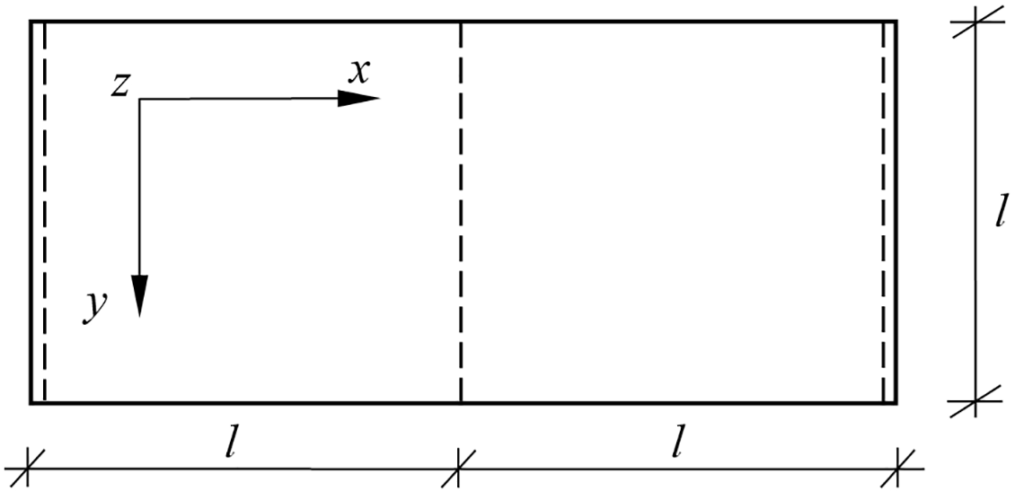
Figure 4: Rectangular plate resting on three parallel continuous supports [18]

4.1.1 The Influence of the Random Parameter of the Collocation Point Position

First, the influence of the collocation point position is investigated. The results of the BEM calculations, presented in Table 1, show the first four natural frequencies calculated for different values of the parameter δ~. Additionally, the first four modes of vibrations are shown in Fig. 5.

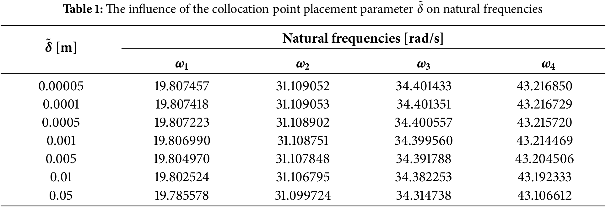
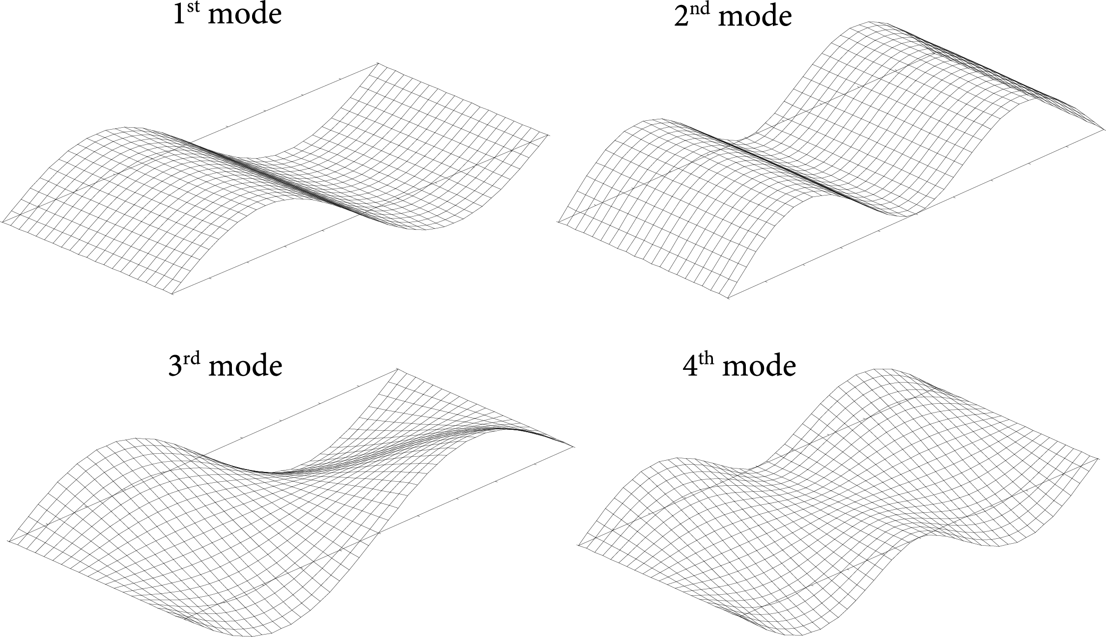
Figure 5: First four modes of vibrations of the considered plate

It can be observed from the data collected in Table 1 that the response of the structure is almost insensitive to changes in the parameter δ~. This is quite good information concerning the fact that this parameter is of a numerical nature, so that the discretization way has a secondary impact on the final results and does not bias the probabilistic response.

The results obtained with the BEM were compared with FEM solutions carried out using the Comlete ABAQUS Environment (CAE), where shell finite elements of the S4R type with a regular mesh of 0.25 m × 0.25 m were adopted. The FEM results are: ω1 = 19.8830990 rad/s, ω2 = 31.13507707 rad/s, ω3 = 34.2798622 rad/s, and ω4 = 43.10509820 rad/s, so that an agreement between the FEM and the BEM solutions is almost perfect. The modes were generated using the “Surfer” program, which was applied to data obtained from the BEM, specifically for the eigenvectors associated with the first four eigenvalues. The eigenvalues and eigenvectors are obtained after solving the standard eigenproblem described by Eq. (21). The method for calculating eigenvalues and determining eigenvectors is based on a procedure written in Fortran 90, which is used here as a ready-made library. Alternatively, any other procedure from any package, such as MATLAB or Octave, may be used.

4.1.2 The Influence of the Random Young’s Modulus and the Plate Thickness

The influence of Young’s modulus, as a basic material constant, and the plate thickness is investigated. The number of deterministic solutions is 21. Young’s modulus varies from 25 to 35 GPa in a regularly ordered manner by 0.5. The fourth-order polynomial fitting was used for both random parameters. LSM obtains these polynomials, coupled with weighted averaging, using weights arranged in the sequence [1, 1, 1, 1, 1, 1, 1, 1, 1, 1, 20, 1, 1, 1, 1, 1, 1, 1, 1, 1, 1]. It is worth noting that this weighting scheme is motivated by the fact that the most important value corresponds to the mean of the input uncertainty. All points are important, although the point corresponding to the mean value receives the most significant weight. It has been documented that such a scheme improves the numerical convergence of all probabilistic characteristics of the structural response under consideration. Next, it is worth checking how the solution behaves when described just by third-degree polynomials, and the number of deterministic solutions is equal to 7. The Young’s modulus varies from 27 to 33 GPa in a regular order, one by one. Similar relations for the random variable in the form of plate thickness and the number of deterministic solutions equal 21; the plate thickness varies from 0.18 to 0.22 m in a regularly ordered manner by 0.002. Analogously as above, the fitting polynomials are obtained by LSM coupled with weighted averaging for weights arranged in the sequence [1, 1, 1, 1, 1, 1, 1, 1, 1, 1, 20, 1, 1, 1, 1, 1, 1, 1, 1, 1, 1]. These curves can be fitted quite efficiently by just three-degree polynomials, and only the seven deterministic solutions as well. The plate thickness varies from 0.17 to 0.23 m in a regularly ordered manner, by one unit. The expected value E(ωi) and coefficient of variation α(ωi), skewness β(ωi), and kurtosis κ(ωi) of the first two natural frequencies (i = 1, 2) have been presented in Figs. 6 and 7 for typical fitting and 21 deterministic solutions, and in Figs. 8 and 9 for weighted fitting and the same number of deterministic solutions. The total number of MC trials is equal to 5 × 105.

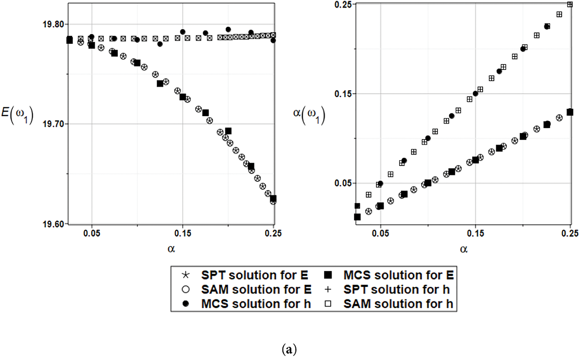
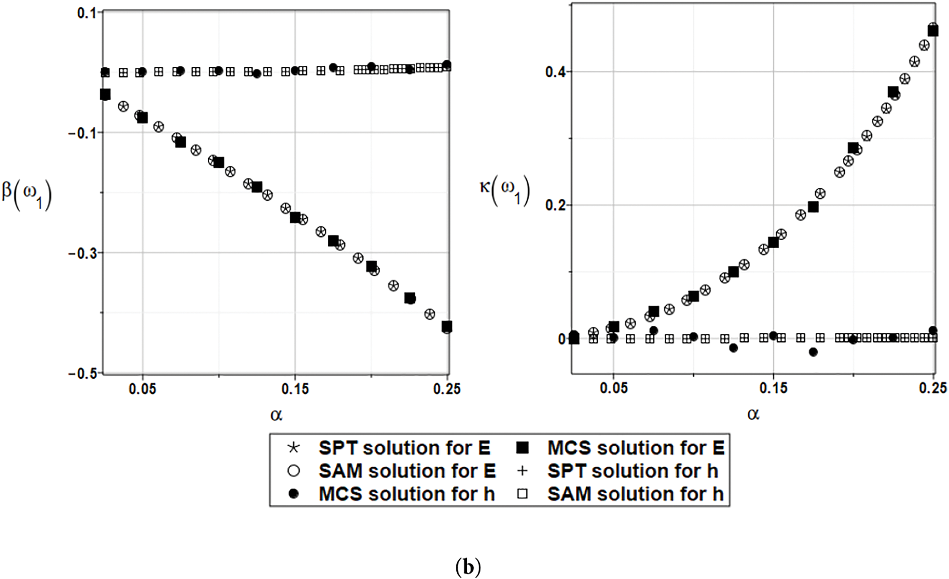
Figure 6: (a) Expected value and coefficient of variation for the first natural frequency and the random distribution of the Young’s modulus and the plate thickness. (b) Skewness and kurtosis for the first natural frequency and the random distribution of the Young’s modulus and the plate thickness

Figure 7: (a) Expected value and coefficient of variation for the second natural frequency and the random distribution of the Young’s modulus and the plate thickness. (b) Skewness and kurtosis for the second natural frequency and the random distribution of the Young’s modulus and the plate thickness

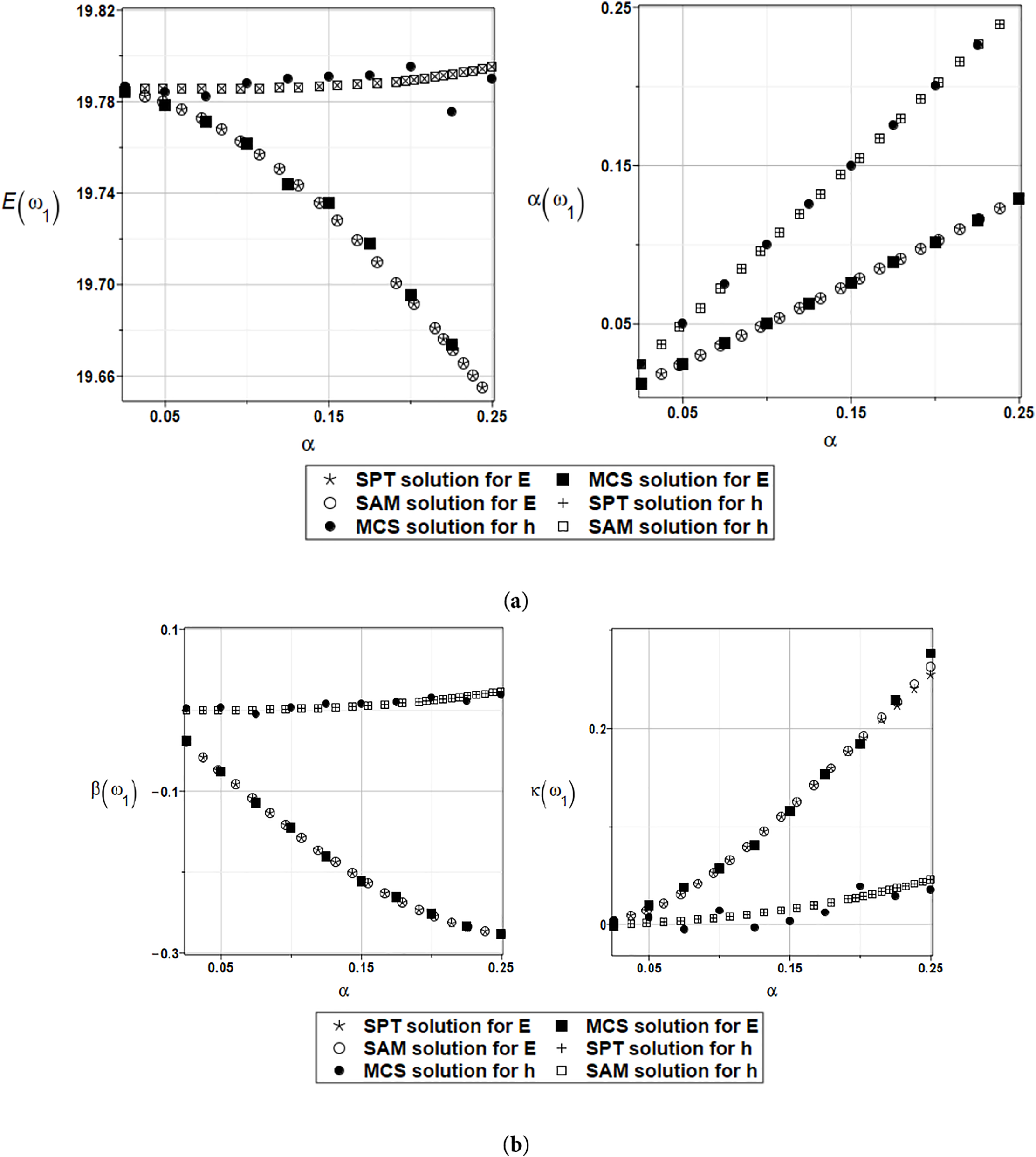
Figure 8: (a) Expected value and coefficient of variation for the first natural frequency and the random distribution of the Young’s modulus and the plate thickness with weighted fitting. (b) Skewness and kurtosis for the first natural frequency and the random distribution of the Young’s modulus and the plate thickness with weighted fitting

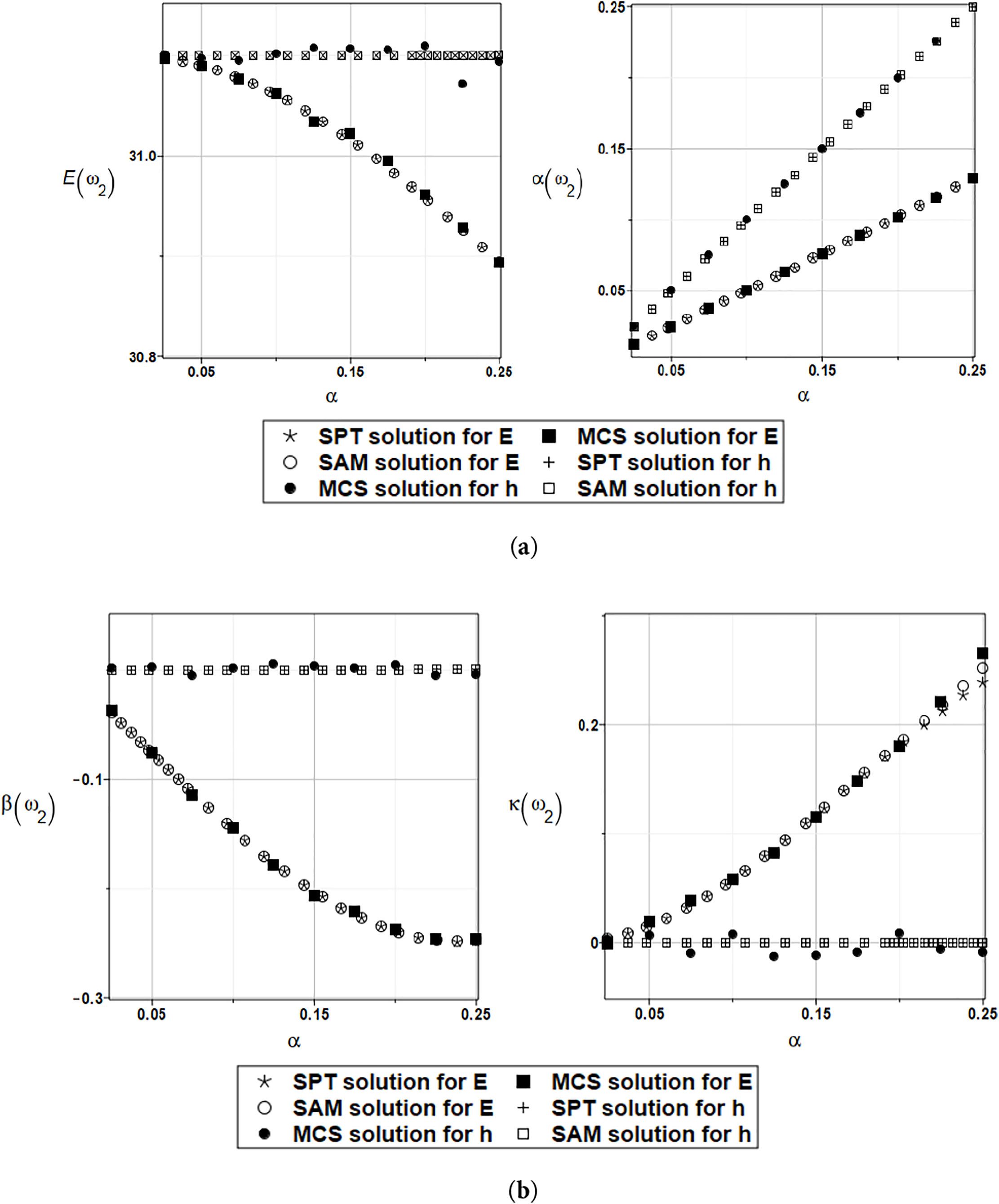
Figure 9: (a) Expected value and coefficient of variation for the second natural frequency and the random distribution of the Young’s modulus and the plate thickness with weighted fitting. (b) Skewness and kurtosis for the second natural frequency and the random distribution of the Young’s modulus and the plate thickness with weighted fitting

As illustrated in Fig. 6a, uncertainty in the plate thickness does not affect the expectation of the first eigenvalue, unlike the randomness in Young’s modulus, which slightly decreases this value. Quite expectedly, a coefficient of variation of the thickness is more influential than the one related to the elastic modulus. It is seen that uncertainty in the first eigenvalue linearly depends on the thickness’s coefficient of variation (CoV), α(ω1)<α(E) so that geometrical uncertainty is definitely more important than the material one. Higher-order statistics shown in Fig. 6b enable us to conclude that the first eigenvalue of the plate has a distribution close to the Gaussian probability density function (PDF) when its thickness is randomized, and is distant from this reference distribution when Young’s modulus is uncertain. It is also observed that the larger the uncertainty in Young’s modulus, the farther the distance of both higher order statistics from the reference value corresponding to the Gaussian distribution, where skewness and kurtosis both equal 0.

The agreement of all three probabilistic methods is very satisfactory. Some discrepancies are observed in the expectations, but they are within the numerical precision of the entire analysis and can therefore be neglected. A contrast of Figs. 6 and 8 relevant to the first eigenvalue and Figs. 7 and 9, corresponding to the second eigenvalue, exhibit that the numerical results show the same trends. However, the values of the response statistics are more concentrated, and the agreement of the three probabilistic methods appears better.

Then, based on relative probabilistic entropy, the so-called structural reliability index can be estimated for the Young’s modulus and the plate thickness. The reliability index is estimated using the SPT and SAM approaches, which employ polynomials of the third order, based on seven deterministic solutions coupled with classic LSM procedures. The results are presented in Figs. 10 and 11, respectively.

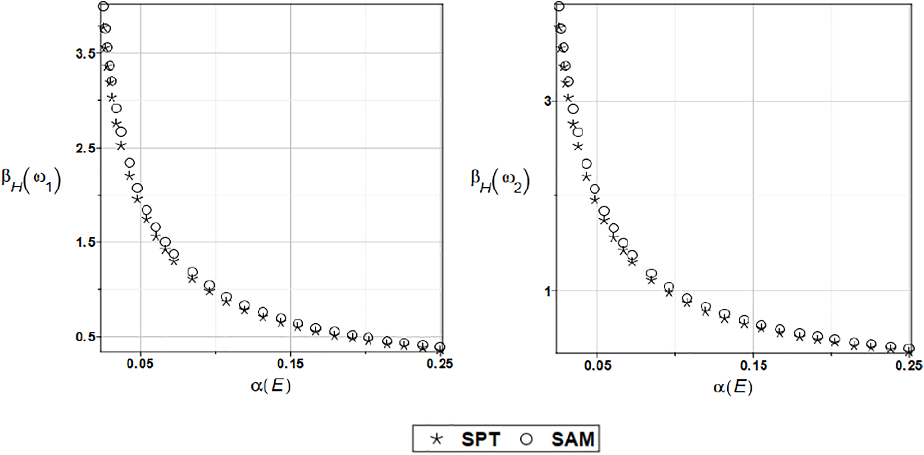
Figure 10: The safety measures for the first and the second natural frequencies and the Gaussian Young’s modulus

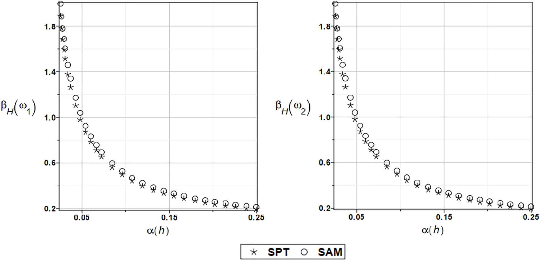
Figure 11: The safety measure for the first and second natural frequencies and Gaussian plate thickness

The reliability indices shown in Figs. 10 and 11 decrease exponentially with increasing uncertainty in both parameters, a result widely available in reliability assessments. Almost the same values are obtained for the first and for the second eigenvalue, correspondingly—see the vertical axes of the left and right diagrams.

It is also observed that statistical material imperfections are significantly less hazardous than geometrical ones, as the reliability index obtained with uncertain thickness is approximately two times smaller than that with random treatment of the plate’s Young’s modulus.

Analogously, a prediction of the solution parametrized with both mean value and standard deviation of the Young’s modulus is presented in Fig. 12, and analogous results related to the uncertainty in the plate thickness are contained in Fig. 13.

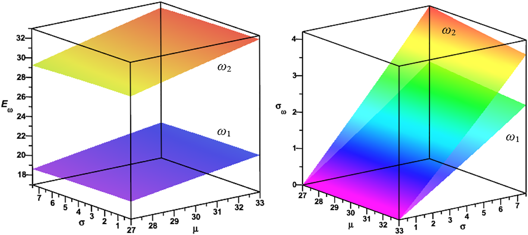
Figure 12: Expected value and standard deviations for the first and the second circular frequencies of natural vibrations for randomly distributed Young’s modulus

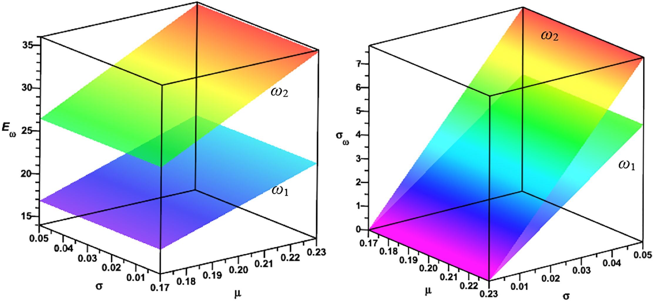
Figure 13: Expected value and standard deviations for the first and the second circular frequencies of natural vibrations for randomly distributed plate thickness

The two above figures show that each time, larger values of the first two probabilistic moments are obtained for the second eigenvalue. It deserves further verification to determine if higher eigenfrequencies exhibit the same property: the higher the eigenfrequency, the higher the statistical moments. It is also observable that the expectations of these eigenvibrations are affected by the expectations of random inputs. Standard deviations of ω1, ω2 and depend finally on the coefficients of variation of Young’s modulus and plate thickness, whereas the expectations play only a secondary role.

A contrast of Figs. 10 and 11 show that larger values of both statistics are obtained while randomizing plate thickness. This means that the thickness of the plate is more critical when optimally designing the thin plate, because a limit function necessary in reliability analysis yields remarkably smaller values than those for material random imperfections.

In many problems, such as experimental ones, it is not possible to have a large set of deterministic data at hand. In such cases, it is necessary to rely on a smaller amount of data. The comparison of the random solution for 7 and 21 deterministic points (solutions) and the fitting function in the form of fourth-degree polynomials obtained using the standard LSM procedure is shown below in Figs. 14 and 15, respectively. In the presented problems, excellent agreement can be observed between the results for 7 and 21 deterministic solutions. This is likely due to the use of fourth-degree polynomials as the response functions. They contain a certain “reserve” for better determination of their derivatives.

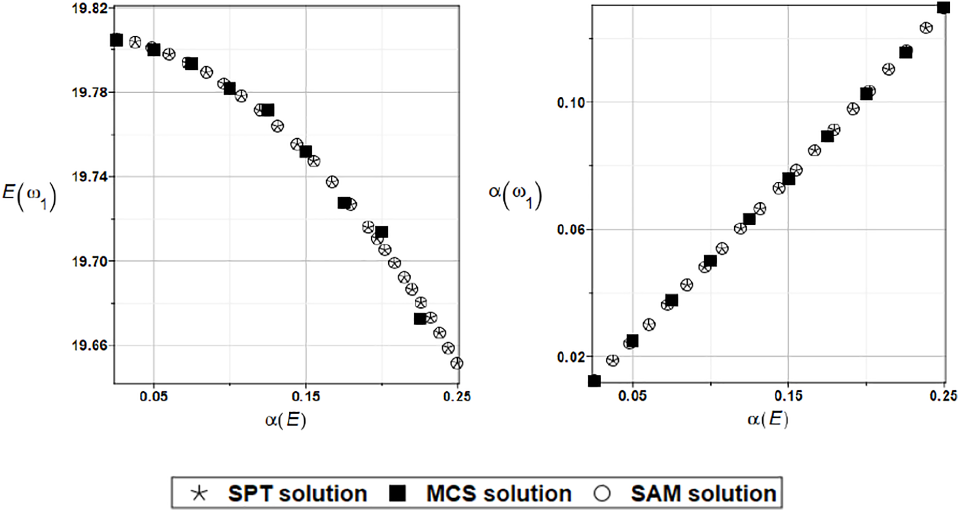
Figure 14: Expected value and coefficient of variation for the first natural frequency and the random distribution of the Young’s modulus and 7 deterministic solutions

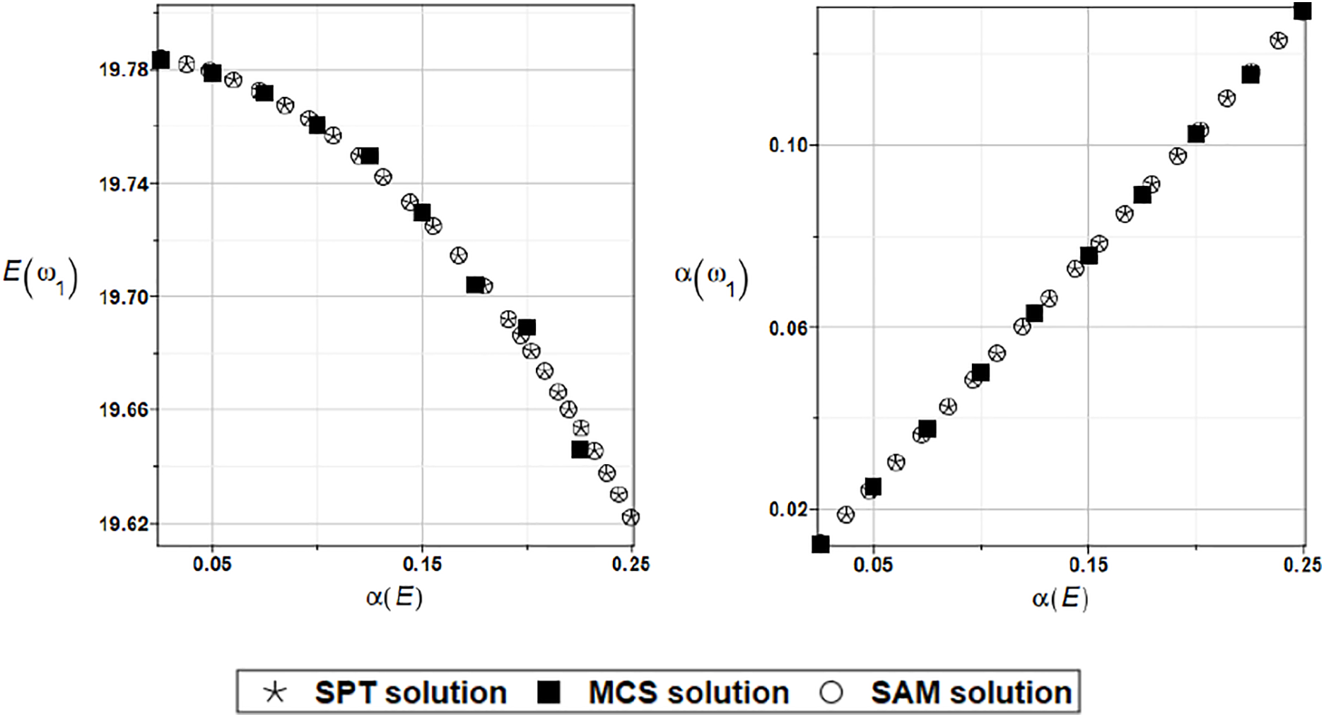
Figure 15: Expected value and coefficient of variation for the first natural frequency and the random distribution of the Young’s modulus and 21 deterministic solutions

4.2 Eigenvibrations of the Rectangular Plate Supported with Four Internal Columns

The plate support scheme analyzed in this numerical example is shown in Fig. 16. The plate edge is divided into 120 boundary elements of equal length, and 225 internal collocation points related to the concentrated masses were introduced. The following material data are assumed: Young’s modulus E = 205.0 GPa, Poisson’s ratio v = 0.3, and material density ρ = 7850 kg/m3 and the plate thickness h = 0.1 m [18].

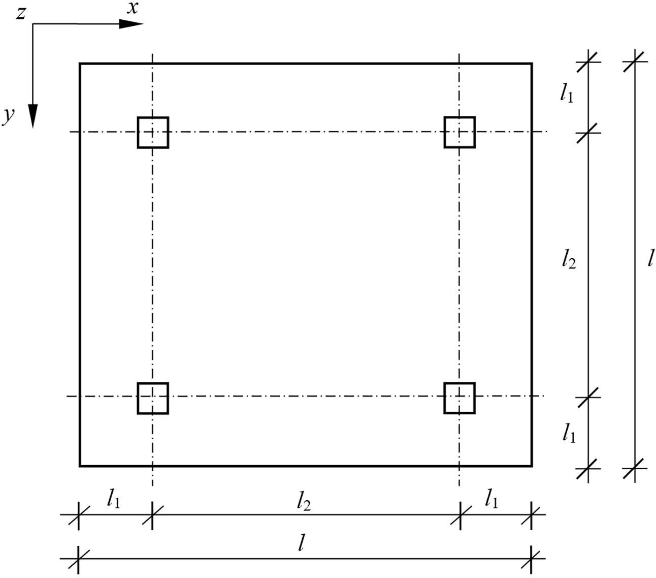
Figure 16: Square plate resting on four symmetric column supports [18]

The dimensions of the column supports are determined based on the dimensions of the plate, a/l=1/30, where l=6.0 m. The location of the geometric centers of the column supports is given by the relation l1/l=0.2.

4.2.1 The Influence of the Random Parameter of the Collocation Point Position

Similarly, as in the first example, the influence of the collocation point position δ~ is investigated. The results of the BEM calculations, as the first four natural frequencies, are shown in Table 2.

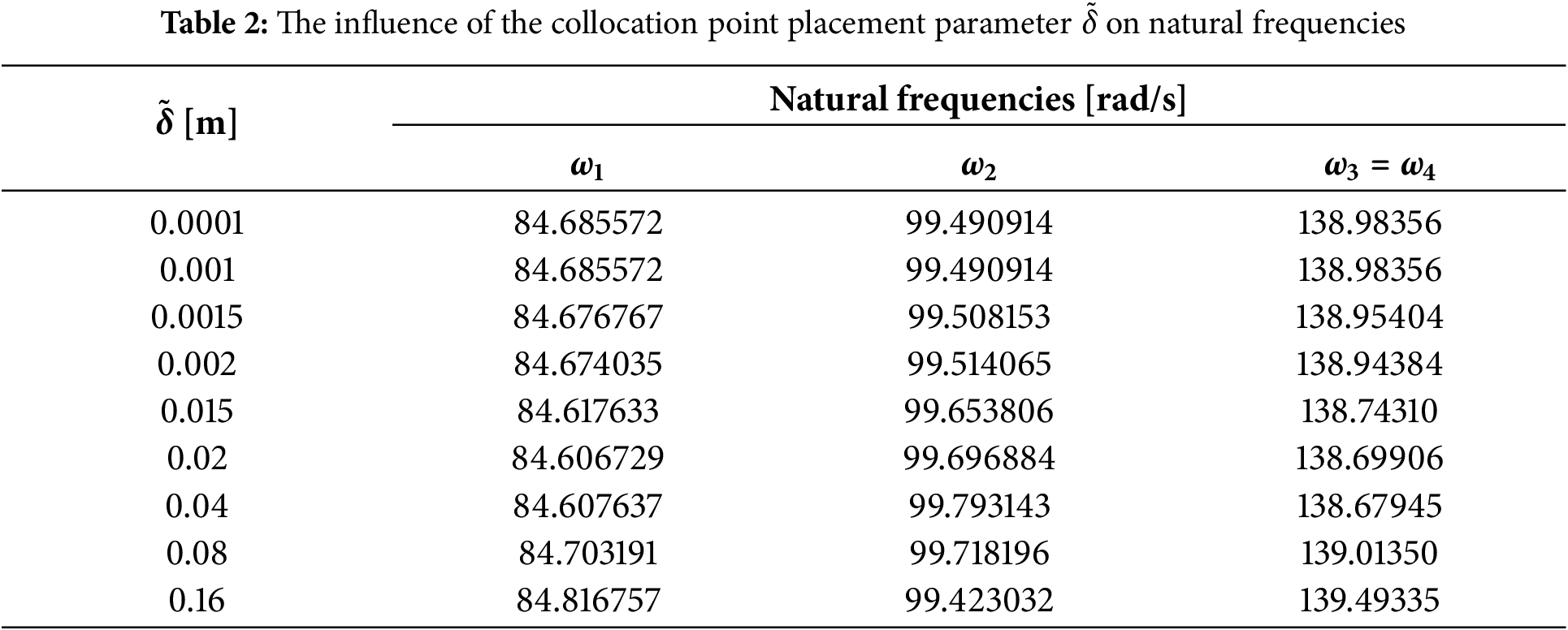
A minimal sensitivity of the structural response to change the δ~ parameter is observed, and the first four modes of vibration are shown in Fig. 17.

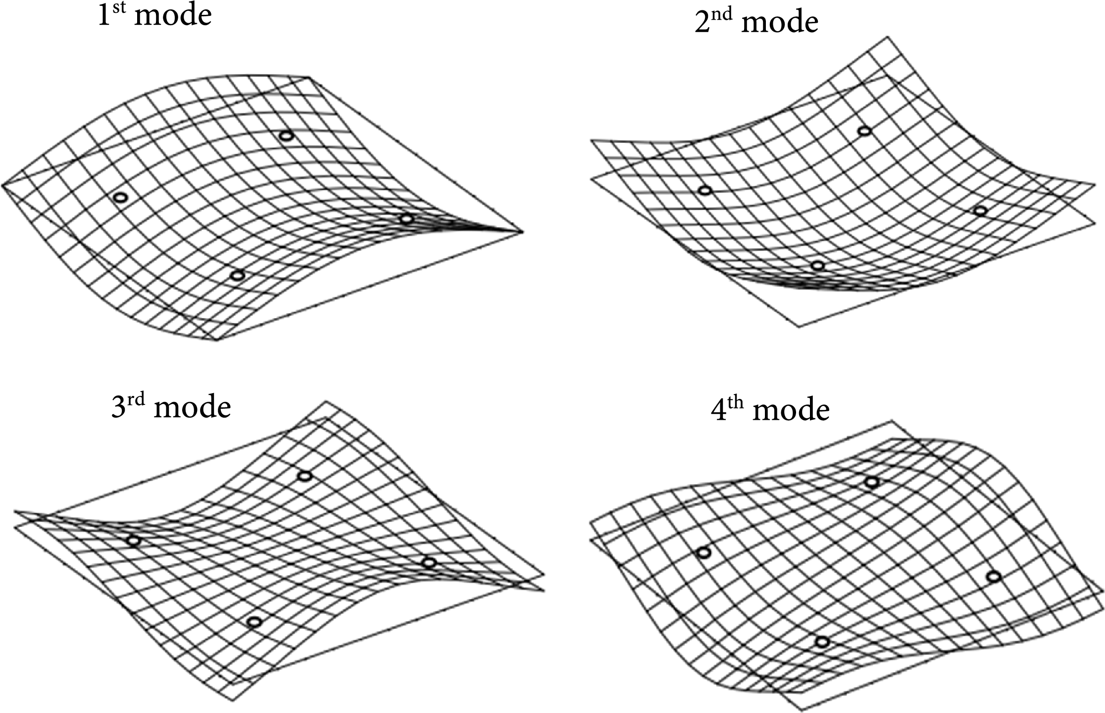
Figure 17: First four modes of vibrations

The obtained BEM results are compared with analytical solutions obtained by Woźnica [37]: ω1 = 84.23757884 rad/s, ω2 = 98.97163776 rad/s, and ω3 = ω4 = 140.897123208 rad/s. The vibration modes were determined identically to those in the previous example Section 4.1.1.

4.2.2 The Influence of the Random Young’s Modulus and the Poisson's Ratio

Initially, the influence of Young’s modulus is investigated. The number of deterministic solutions is 21. Young’s modulus varies from 195 to 215 GPa in a regular ordered manner by 1. The fourth-order polynomial fittings are used for both random parameters in this case. LSM obtains the fitting polynomials coupled with weighted averaging, where the weights are arranged in the sequence [0.5, 0.5, 0.5, 1, 1, 1, 1, 1, 1, 1, 17, 1, 1, 1, 1, 1, 1, 1, 0.5, 0.5, 0.5]. In this example, the study will investigate how the solution behaves when third-degree polynomials and a set of deterministic solutions, each equal to 7, are applied. The Young modulus varies from 190 to 220 GPa in a regularly ordered manner, every five units.

The following random variable is the Poisson’s ratio, and the number of deterministic solutions is also equal to 21. Poisson’s ratio varies from 0.2 to 0.4 in a regularly ordered manner, incrementing by 0.01. The fitting polynomials are determined with the LSM coupled with weighted averaging for weights arranged in the sequence [0.5, 0.5, 0.5, 1, 1, 1, 1, 1, 1, 1, 17, 1, 1, 1, 1, 1, 1, 1, 0.5, 0.5, 0.5]. The polynomials of the third order are estimated using the classic LSM approach. Here, the Poisson’s ratio varies from 0.21 to 0.39 in a regularly ordered manner, every three units. The expected value E(ωi) and coefficient of variation α(ωi), skewness β(ωi), and kurtosis κ(ωi) of the first two natural frequencies (i = 1, 2) have been presented in Figs. 18 and 19 for typical fitting and 21 deterministic solutions, and in Figs. 20 and 21 for weighted fitting and the same number of trial solutions; the total number of Monte Carlo simulations is equal to 5 × 105.

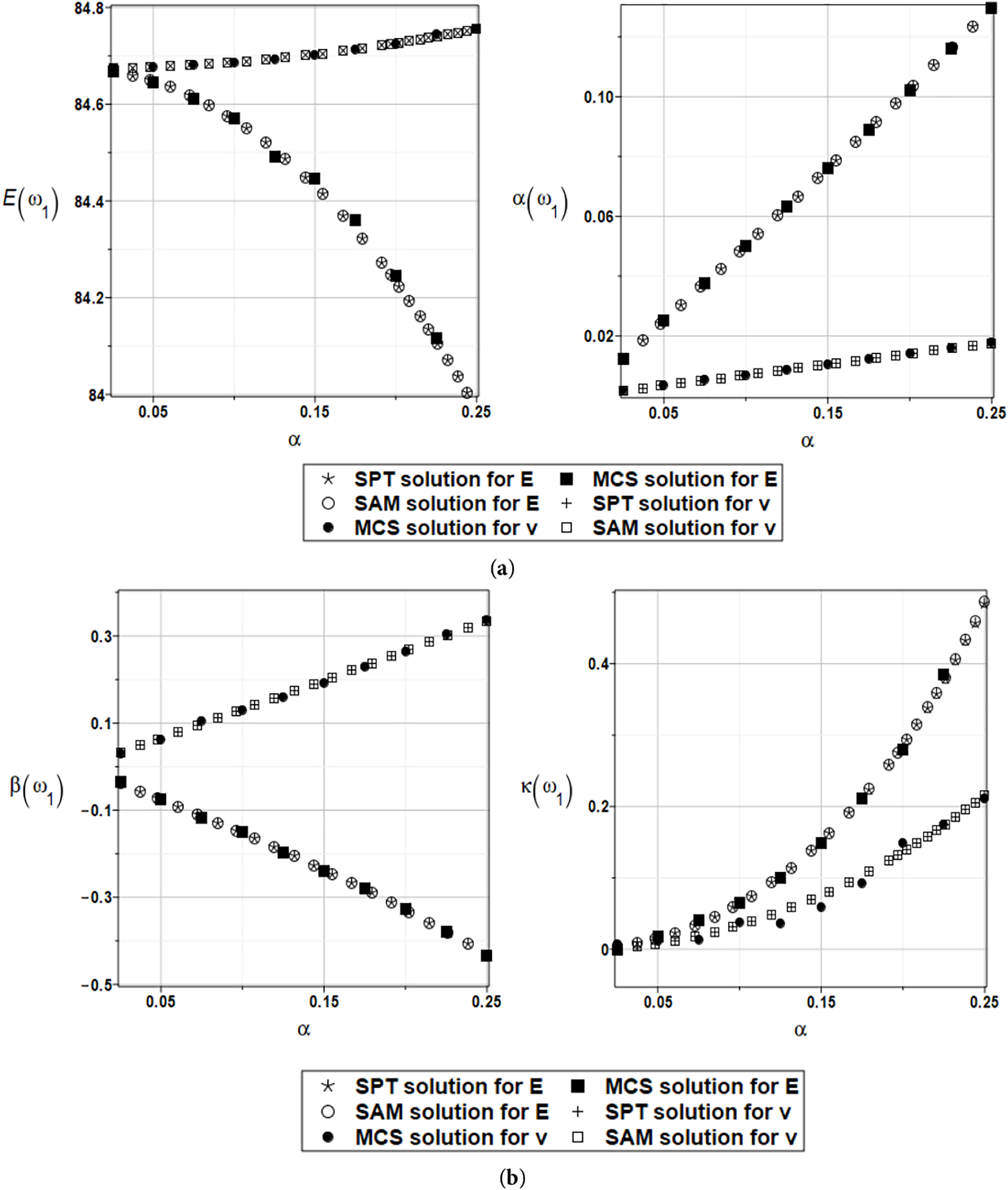
Figure 18: (a) Expected value and coefficient of variation for the first natural frequency and the random distribution of the Young’s modulus and the Poisson’s ratio. (b) Skewness and kurtosis for the first natural frequency and the random distribution of the Young’s modulus and the Poisson’s ratio

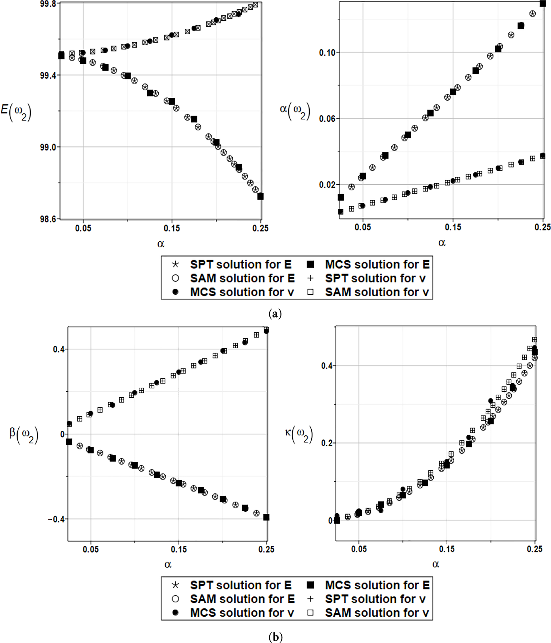
Figure 19: (a) Expected value and coefficient of variation for the second natural frequency and the random distribution of the Young’s modulus and the Poisson’s ratio. (b) Skewness and kurtosis for the second natural frequency and the random distribution of the Young’s modulus and the Poisson’s ratio

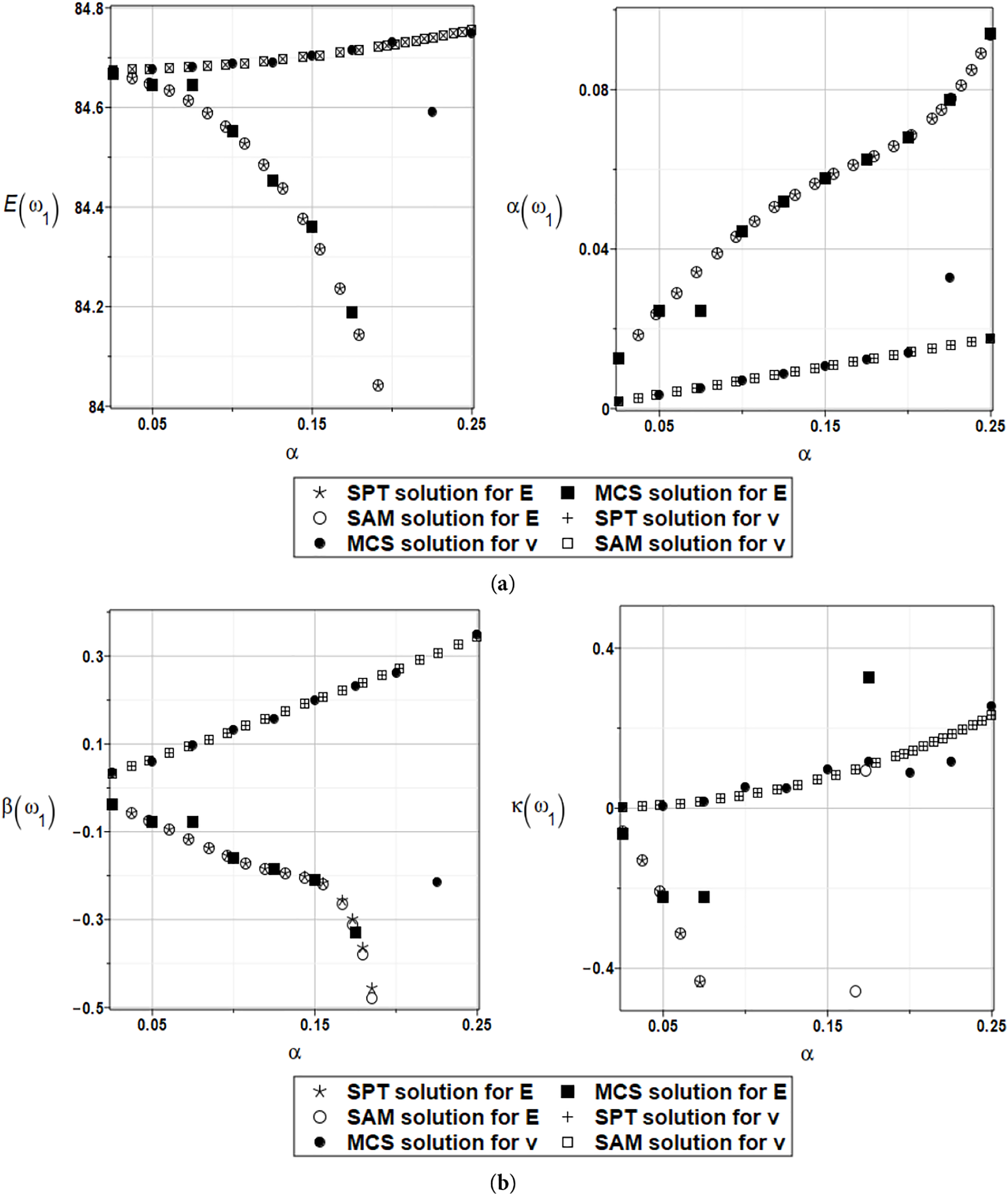
Figure 20: (a) Expected value and coefficient of variation for the first natural frequency and the random distribution of the Young’s modulus and the Poisson’s ratio with weighted fitting. (b) Skewness and kurtosis for the first natural frequency and the random distribution of the Young’s modulus and the Poisson’s ratio with weighted fitting

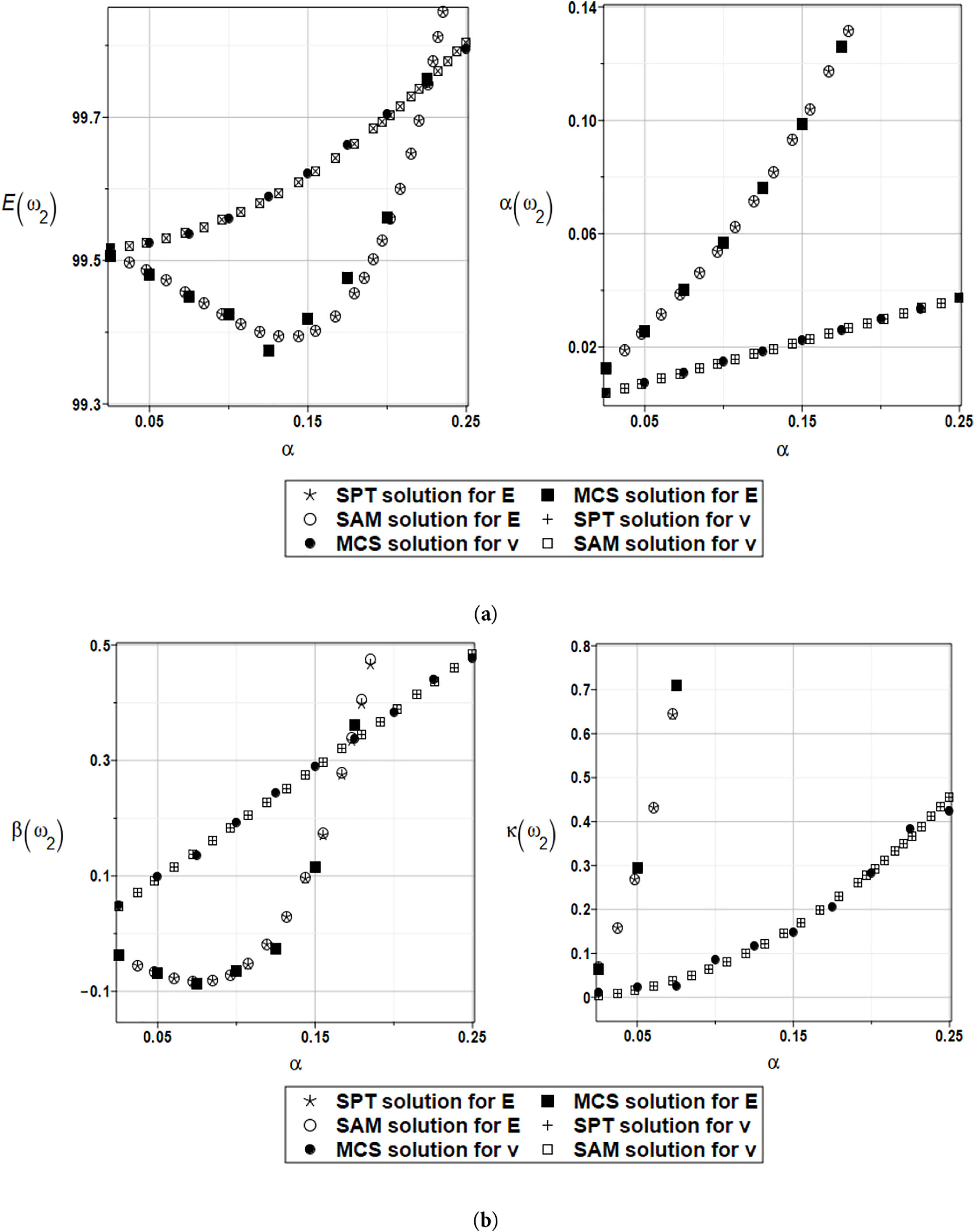
Figure 21: (a) Expected value and coefficient of variations for the second natural frequency and the random distribution of the Young’s modulus and the Poisson’s ratio with weighted fitting. (b) Skewness and kurtosis for the second natural frequency and the random distribution of the Young’s modulus and the Poisson’s ratio with weighted fitting

The most important conclusions coming from Figs. 18 and 19 is that the agreement of all three probabilistic numerical methods is almost perfect for both random inputs; it is specifically essential in the case of Poisson’s ratio, because this parameter usually causes remarkable problems due to its complex function in the elasticity tensor. Therefore, the generalized stochastic perturbation method can be recommended for further computations as the fastest technique, yielding the same numerical error as the reference methods. Quite expectedly, both material parameters cause non-Gaussian first and second eigenvalues, which confirms the previous case study results: the larger the input uncertainty level, the greater the distance of the resulting PDFs from the Gaussian reference bell-shaped curve. This indicates that fourth-moment numerical analysis is necessary.

Additionally, the influence of Poisson’s ratio uncertainty is significant (cf. the right graphs of Figs. 18a and 19a), as even the expected values are substantially affected by the coefficient of variation of this parameter. This is unusual in probabilistic mechanics in the linear elastic regime, where usually material uncertainty has no impact on the expectations of quasi-static structural response. It is also noticeable that the kurtosis for both eigenvalues holds non-negative values only, regardless of the input uncertainty level, so that the resulting PDFs are more concentrated about their mean values than for the Gaussian reference PDF. Poisson’s ratio is found in the denominator of the plate stiffness parameter and appears as a squared term. In solutions such as the expected value, some slight nonlinearity can be observed, while skewness typically produces results that form a linear dependence.

The weighted fitting documented in Figs. 20 and 21 brings remarkable numerical discrepancies in the determination of the first four probabilistic characteristics of the first two eigenvalues. Firstly, it is evident that the total number of random samples in the Monte Carlo scheme requires further improvement due to the significant variations in the results from the prominent trends as the input uncertainty level increases. Although the main conclusions remain generally the same as for the non-weighted Least Square Method (LSM) polynomial bases application, the resulting functions of at least the coefficients of variation (right graphs in Figs. 17a and 18a) become apparently nonlinear, monotonous, but not necessarily convex.

Not surprisingly, the expectations of the second eigenvalue also undergo some unusual variations, as seen in Fig. 18a, left graph. The skewness and kurtosis also exhibit some unusual fluctuations, so that replacing the traditional LSM with the weighted least square method (WLSM) does not yield more stable results and warrants further computational studies, likely with different orders of approximating polynomials.

The reliability index has been estimated using the SPT and SAM approaches, which employ polynomials of the third order, based on seven deterministic solutions coupled with classic LSM procedures for the Young’s modulus. The results are presented in Figs. 22 and 23, respectively. The resulting reliability curves exhibit the same properties as in the previous case—the exponential decay, together with the input uncertainty level, is quite clear.

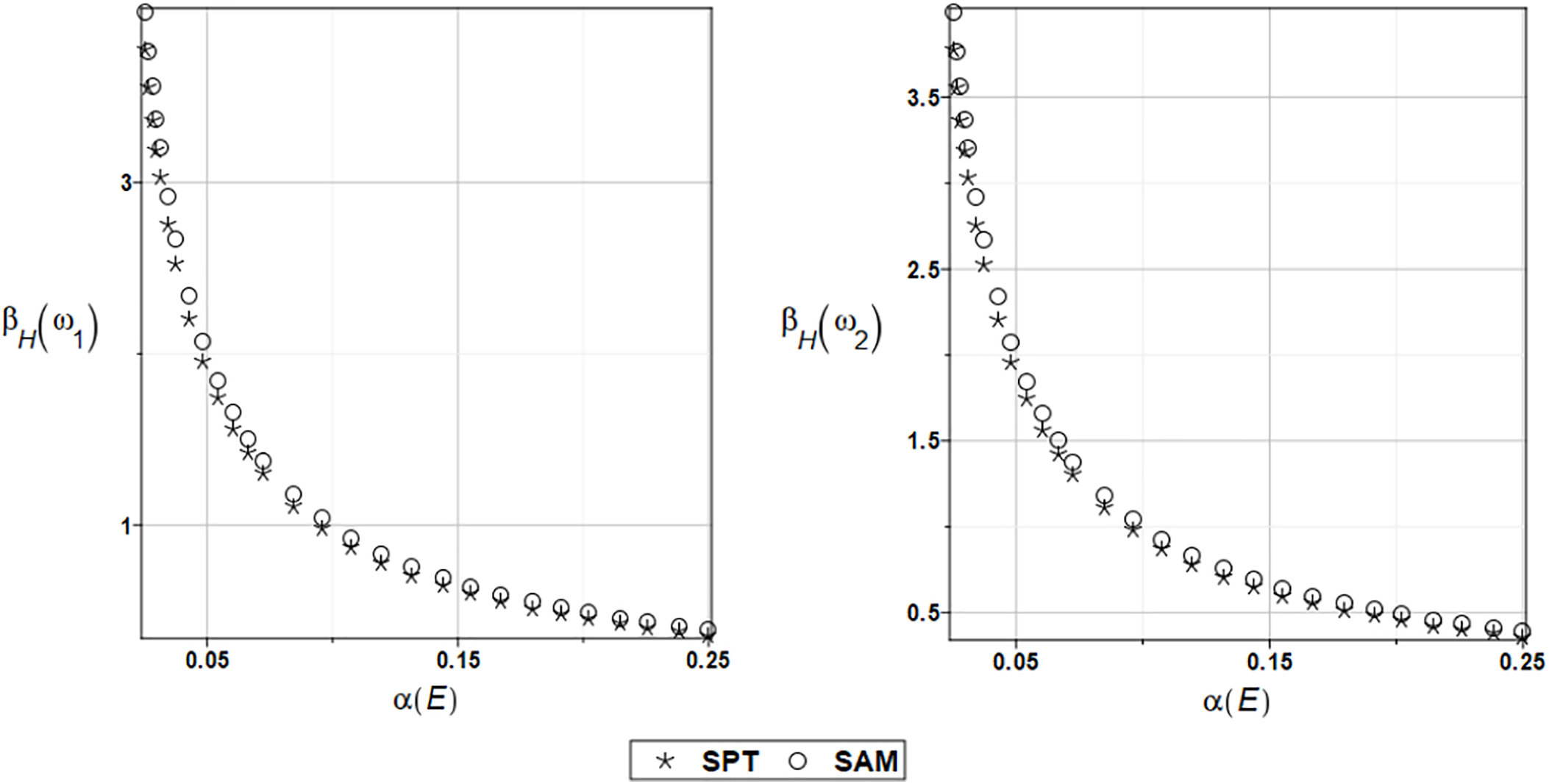
Figure 22: The safety measure for the first and second natural frequencies and randomly distributed Young’s modulus

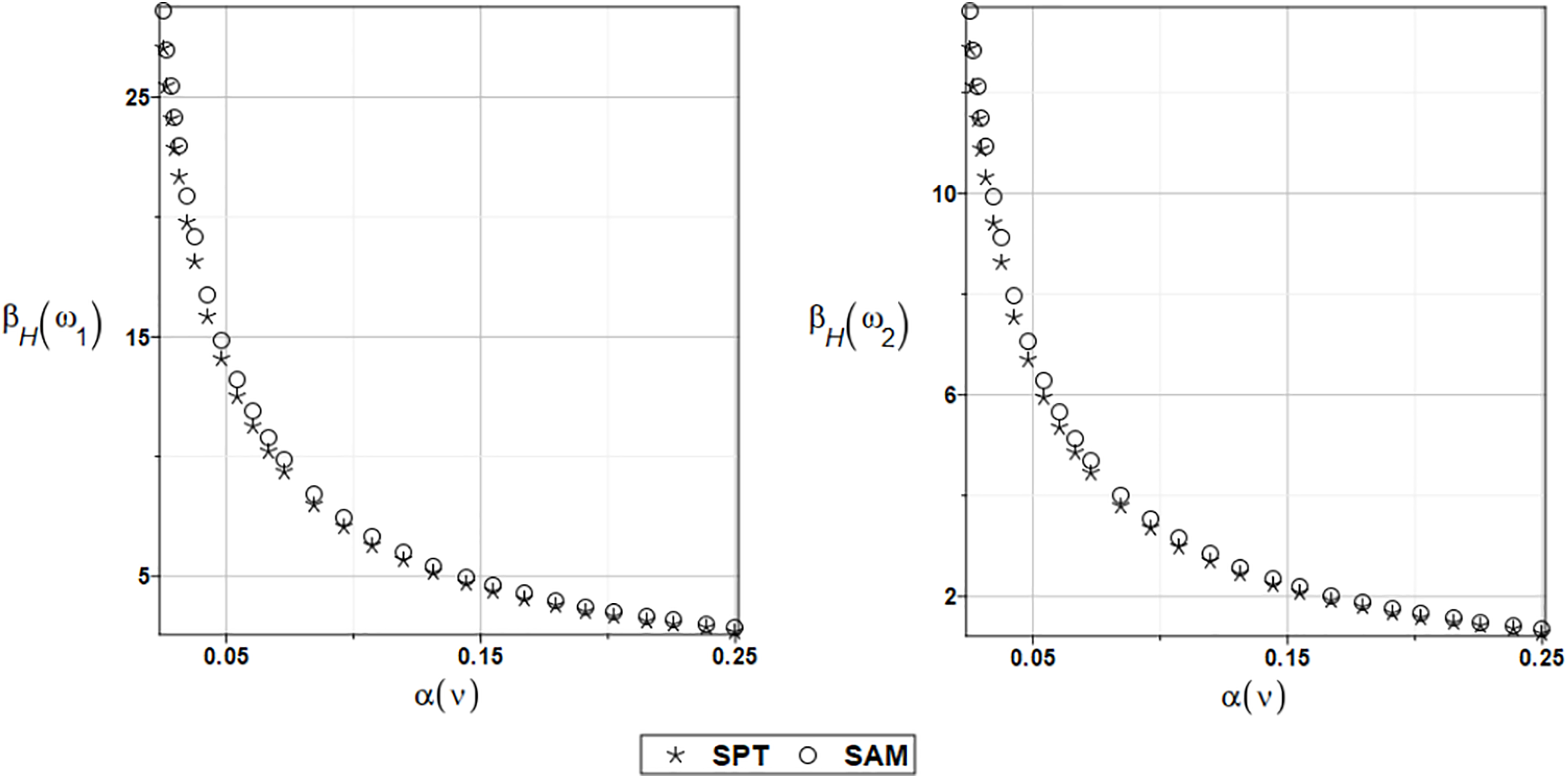
Figure 23: The safety measure for the first and second natural frequencies and a randomly distributed Poisson’s ratio

The coincidence of the two probabilistic numerical methods is also apparent, although the semi-analytical strategy yields slightly larger values of the reliability index; therefore, a less favorable stochastic perturbation method would be recommended once more. The reliability indices have remarkably smaller values in the case of the Young’s modulus uncertainty than for the Poisson’s ratio. Therefore, considering this second parameter in reliability assessment is definitely less important. Additionally, it is observed that the reliability curves cross the admissible limit as the CoVs of the Young’s modulus increase, making the precise identification of the statistical moments of this variable during the experimental test mandatory.

The polynomials of the third order have been used to estimate a two-parametric solution in the form of expected values and standard deviation for the predicted domain of the mean value and standard deviation of the arguments for Young’s modulus. The results of calculations for the first and the second natural frequency for the Young modulus are shown in Fig. 24, and for Poisson’s ratio in Fig. 25. As it was seen in the first experiment, the expected values of both eigenvalues are more affected by the expectations of the given material uncertainties. In contrast, the fluctuations in their standard deviations are the result of variations in the standard deviations. Generally, as before, larger output statistics are observed for the second eigenvalue than for the first, which is more interesting in terms of the resulting standard deviations.

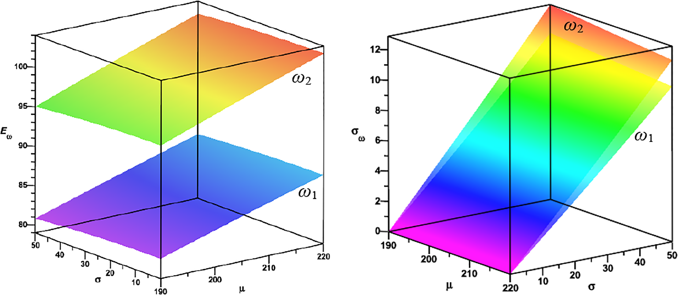
Figure 24: Expected value and standard deviations for the first and the second natural frequencies of natural vibrations for randomly distributed Young’s modulus

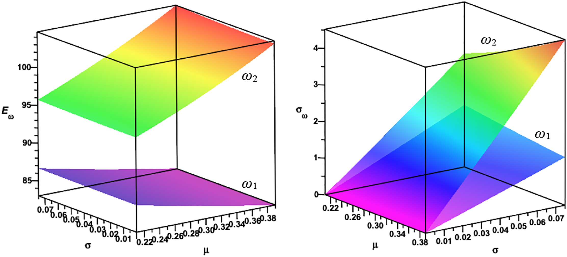
Figure 25: Expected value and standard deviations for the first and the second natural frequencies of natural vibrations for randomly distributed Poisson’s ratios

5  Discussion

Next to sensitivity analysis, random analysis is a significant branch of solution forecasting, as well as estimating the reliability measure of a structure or its elements. For example, thickness uncertainty is of great practical importance in the context of possible corrosion processes of plate elements—the simplest example is a steel plate. The structural response fitting curves were made using polynomial functions, and the Gaussian probability density function was assumed.

A novelty is the random approach to the Kirchhoff plate bending problem using the Boundary Element Method for a modified (simplified) construction of integral boundary equations for the dynamics of a plate with internal supports, both continuous and columnar. The random approach places slightly more emphasis on solving the problem deterministically, where solutions are provided for three independent methods: SAM, SPT, and MCs. The fitting curves are determined classically using polynomials, typical fitting, and weighted fitting. Additionally, solutions in the form of random surfaces in the space defined by the expected value and standard deviation of the design parameter were determined, and the so-called reliability measure was estimated based on relative probabilistic entropy.

Determining the random matching function is the most critical step in random analysis. Polynomial functions are best suited for this purpose. The degree of these polynomials depends on the influence of the random parameter on the solution. Polynomials of the third degree are often sufficient, but not always. It is good to assume a certain “reserve” associated with the differentiation of such functions and work on polynomials of the fourth degree. Fitting a polynomial function to a region defined by a finite number of deterministic points (solutions) can be done using the classical LSM or by using weighted averages. The adoption of weights corresponding to deterministic solutions is, in its own way, a separate random problem. For example, weights of the type 10 × 1, 20, and 10 × 1 did not always give the correct fit for higher probabilistic moments. In the presented problems, the weights were adopted by trial and error. Here, the next issue may be formulated, i.e., optimizing the weight values for the fitting polynomials. The proposed approach obviously has its limitations. The deterministic problem itself is linear, both materially and geometrically. In the random approach, the weights for the fitting curves are selected empirically, which requires a larger number of deterministic points (solutions). Using the Monte Carlo approach, on the other hand, requires a large number of trials, which significantly increases computational time.

6  Conclusion

Random vibrations of thin (Kirchhoff) plates, considering internal continuous and column supports, have been investigated and solved using the Stochastic Boundary Element Method (SBEM) in direct terms, with the non-singular formulation of the boundary and domain integral equations, and the introduction of simplified boundary conditions. This formulation allows for a significant simplification of the BEM calculation algorithm. The role of corner forces is played here by the force values assigned to the nodes of the boundary elements located near the corner. To simplify the calculation algorithm, no corner forces or equivalent transverse forces are introduced. The tangential angle of rotation at the edge of the plate is expressed by the displacements (deflections) of three adjacent nodes, and in the case of boundary elements of the constant type, deflections at the geometric center of gravity of the element. Hence, the non-singular formulation of integral boundary equations is very convenient. All this significantly simplifies the BEM calculation algorithm.

Three independent approaches were used for random calculations: semi-analytical method (SAM), perturbative (SPT), and Monte Carlo Simulation (MCs), with the fitting curves determined classically using the least square method (LSM) and additionally using weighted least square method (WLSM). Slight differences in the random solutions can be observed, for example, for the expected value as the most interesting solution. The simplest probabilistic approach is the SAM, which allows us to derive probabilistic estimators in analytical terms. The SPT yields results that are almost identical to those obtained by the SAM approach. This is due to the degree of accuracy of the Taylor series expansion of the probabilistic moment expressions. Finally, the MCs approach requires the most computational time.

The presented problems have their limitations, primarily those inherent to the direct BEM approach itself, e.g., for purely linear problems, plates of constant thickness. These limitations can largely be avoided by using the Analog Equation Method (AEM) coupled with the BEM. The presented examples can be used in engineering practice, for example to describe random vibrations of plane girders (steel, welded girders) of bridge structures or plate-column structural systems. In future research, a good alternative to the Least Squares Method, in its classical and weighted schemes, can be seen in the broader application of machine learning methodology, where specifically programmed computer programs are capable of determining the best approximation from given data sets. Additionally, it is not necessary to have a polynomial form, which guarantees fast probabilistic convergence but does not necessarily lead to an intuitively convenient approximation. This is particularly the case for plates resting on an elastic foundation or those subjected to given stiffness supports, where exponential functions are more appropriate.

Acknowledgement: This paper has been written in the framework of the research grant OPUS no. 2021/41/B/ST8/02432 entitled Probabilistic entropy in engineering computations sponsored by The National Science Center in Poland and Institute of Structural Analysis of Poznan University of Technology, internal research grant 0411/SBAD/0010.

Funding Statement: This paper has been funded by research grant OPUS no. 2021/41/B/ST8/02432 entitled Probabilistic entropy in engineering computations sponsored by The National Science Center in Poland, and also by the Institute of Structural Analysis of Poznan University of Technology in the framework of the internal research grant 0411/SBAD/0010.

Author Contributions: The authors confirm contribution to the paper as follows: Conceptualization, Michał Guminiak and Marcin Kamiński; methodology, Michał Guminiak and Marcin Kamiński; software, Michał Guminiak and Marcin Kamiński; validation, Marcin Kamiński; formal analysis, Michał Guminiak and Marcin Kamiński; investigation, Michał Guminiak and Marcin Kamiński; resources, Michał Guminiak and Marcin Kamiński; data curation, Michał Guminiak and Marcin Kamiński; writing—original draft preparation, Michał Guminiak; writing—review and editing, Marcin Kamiński; visualization, Michał Guminiak and Marcin Kamiński; supervision, Marcin Kamiński; project administration, Marcin Kamiński; funding acquisition, Marcin Kamiński. All authors reviewed the results and approved the final version of the manuscript.

Availability of Data and Materials: Data available on request from the authors.

Ethics Approval: Not applicable.

Conflicts of Interest: The authors declare no conflicts of interest to report regarding the present study.

References

1. Kellogg OD. Foundations of potential theory. New York, NY, USA: Dover Publications; 1953. [Google Scholar]

2. Kupradze BD. Potential methods in elasticity theory. Moscow, Russia: Fizmatgiz; 1963. (In Russian). [Google Scholar]

3. Michlin SG. Multivariable singular integrals and integral equations. Moscow, Russia: Fizmatgiz; 1963. (In Russian). [Google Scholar]

4. Jaswon MA. Integral equations method in potential theory I. Proc R Soc A. 1963;275(1360):23–32. [Google Scholar]

5. Symm GT. Integral equation method in potential theory II. Proc R Soc A. 1963;275(1360):33–46. [Google Scholar]

6. Stern M. A general boundary integral formulation for the numerical solution of plate bending problems. Int J Solids Struct. 1979;15(10):769–82. doi:10.1016/0020-7683(79)90003-9. [Google Scholar] [CrossRef]

7. Altiero NJ, Sikarskie DL. A boundary integral method applied to plates of arbitrary plan form. Comput Struct. 1978;9(2):163–8. doi:10.1016/0045-7949(78)90134-7. [Google Scholar] [CrossRef]

8. Bèzine G, Gamby DA. A new integral equations formulation for plate bending problems. In: Advances in boundary element method. London, UK: Pentech Press; 1978. [Google Scholar]

9. El-Zafrany A, Debbih M, Fadhil S. A modified Kirchhoff theory for boundary element bending analysis of thin plates. Int J Solids Struct. 1994;31(21):2885–99. doi:10.1016/0020-7683(94)90057-4. [Google Scholar] [CrossRef]

10. Burczyński T. The boundary element method in mechanics. Warsaw, Poland: Scientific and Technical Publishing House; 1995. [Google Scholar]

11. Katsikadelis JT. A boundary element solution to the vibration problem of plates. J Sound Vib. 1990;141(2):313–22. doi:10.1016/0022-460x(90)90842-n. [Google Scholar] [CrossRef]

12. Katsikadelis JT, Sapountzakis EJ, Zorba EG. A BEM approach to static and dynamic analysis of plates with internal supports. Comput Mech. 1990;7(1):31–40. doi:10.1007/BF00370055. [Google Scholar] [CrossRef]

13. Providakis CP, Beskos DE. Dynamic analysis of plates by boundary elements. Appl Mech Rev. 1999;52(7):213–36. doi:10.1115/1.3098936. [Google Scholar] [CrossRef]

14. Katsikadelis JT, Sapountzakis EJ. A BEM solution to dynamic analysis of plates with variable thickness. Comput Mech. 1991;7(5):369–79. doi:10.1007/BF00350166. [Google Scholar] [CrossRef]

15. Katsikadelis JT, Yotis AJ. A new boundary element solution of thick plates modelled by Reissner’s theory. Eng Anal Bound Elem. 1993;12(1):65–74. doi:10.1016/0955-7997(93)90070-2. [Google Scholar] [CrossRef]

16. Wen PH, Aliabadi MH, Young A. A boundary element method for dynamic plate bending problems. Int J Solids Struct. 2000;37(37):5177–88. doi:10.1016/s0020-7683(99)00187-0. [Google Scholar] [CrossRef]

17. Katsikadelis J, Babouskos N. Nonlinear flutter instability of thin damped plates: a solution by the analog equation method. J Mech Solids Struct. 2009;4(7–8):1395–414. doi:10.2140/jomms.2009.4.1395. [Google Scholar] [CrossRef]

18. Guminiak M. The boundary element method in the analysis of plates. Poznań, Poland: Poznań University of Technology Publishing House; 2016. (In Polish). [Google Scholar]

19. Kamiński M. Iterative scheme in determination of the probabilistic moments of the structural response in the Stochastic perturbation-based boundary element method. Comput Struct. 2015;151(3):86–95. doi:10.1016/j.compstruc.2015.01.017. [Google Scholar] [CrossRef]

20. Wang G, Guo F. A stochastic boundary element method for piezoelectric problems. Eng Anal Bound Elem. 2018;95(13):248–54. doi:10.1016/j.enganabound.2018.08.002. [Google Scholar] [CrossRef]

21. Guminiak M, Kamiński M. On semi-analytical stochastic boundary element method and its application to eigenproblem of thin elastic plate immersed into a fluid. Eng Anal Bound Elem. 2022;134(1963):219–30. doi:10.1016/j.enganabound.2021.10.003. [Google Scholar] [CrossRef]

22. Karakostas CZ, Manolis GD. Dynamic response of tunnels in stochastic soils by the boundary element method. Eng Anal Bound Elem. 2002;26(8):667–80. doi:10.1016/s0955-7997(02)00034-6. [Google Scholar] [CrossRef]

23. Zhang N, Yao L, Jiang G. A coupled finite element-least squares point interpolation/boundary element method for structure-acoustic system with stochastic perturbation method. Eng Anal Bound Elem. 2020;119(5–6):83–94. doi:10.1016/j.enganabound.2020.07.010. [Google Scholar] [CrossRef]

24. Su C, Zhao S, Ma H. Reliability analysis of plane elasticity problems by stochastic spline fictitious boundary element method. Eng Anal Bound Elem. 2012;36(2):118–24. doi:10.1016/j.enganabound.2011.07.015. [Google Scholar] [CrossRef]

25. Su C, Xu J. Reliability analysis of Reissner plate bending problems by stochastic spline fictitious boundary element method. Eng Anal Bound Elem. 2015;51(3–4):37–43. doi:10.1016/j.enganabound.2014.10.006. [Google Scholar] [CrossRef]

26. Su C, Zheng C. Probabilistic fracture mechanics analysis of linear-elastic cracked structures by spline fictitious boundary element method. Eng Anal Bound Elem. 2012;36(12):1828–37. doi:10.1016/j.enganabound.2012.06.006. [Google Scholar] [CrossRef]

27. Su C, Qin Z, Fan X, Xu Z. Stochastic spline fictitious boundary element method for random vibration analysis of plane elastic problems with structural uncertainties. Probab Eng Mech. 2017;49(11):22–31. doi:10.1016/j.probengmech.2017.08.003. [Google Scholar] [CrossRef]

28. Chowdhury MS, Song C, Gao W. Probabilistic fracture mechanics by using Monte Carlo simulation and the scaled boundary finite element method. Eng Fract Mech. 2011;78(12):2369–89. doi:10.1016/j.engfracmech.2011.05.008. [Google Scholar] [CrossRef]

29. Chowdhury MS, Song C, Gao W. Probabilistic fracture mechanics with uncertainty in crack size and orientation using the scaled boundary finite element method. Comput Struct. 2014;137(5):93–103. doi:10.1016/j.compstruc.2013.03.002. [Google Scholar] [CrossRef]

30. Do DM, Gao W, Saputra AA, Song C, Leong CH. The stochastic Galerkin scaled boundary finite element method on random domain. Numer Meth Eng. 2017;110(3):248–78. doi:10.1002/nme.5354. [Google Scholar] [CrossRef]

31. Kamiński M, Vaccaro MS, Barretta R. On a stochastic model of nonlocal elastic beams using the generalized perturbation method. Probab Eng Mech. 2025;81(1):103803. doi:10.1016/j.probengmech.2025.103803. [Google Scholar] [CrossRef]

32. Schiantella M, Cluni F, Gusella V. Geometrical uncertainties influence on the failure load estimation of lattice structures. Probab Eng Mech. 2024;76(76):103636. doi:10.1016/j.probengmech.2024.103636. [Google Scholar] [CrossRef]

33. Huang Z, Beer M. Probability distributions for dynamic and extreme responses of linear elastic structures under quasi-stationary harmonizable loads. Probab Eng Mech. 2024;75:103590. doi:10.1016/j.probengmech.2024.103590. [Google Scholar] [CrossRef]

34. Geisler H, Junker P. Uncertainty quantification for viscoelastic composite materials using time-separated stochastic mechanics. Probab Eng Mech. 2024;76(5):103618. doi:10.1016/j.probengmech.2024.103618. [Google Scholar] [CrossRef]

35. Huang X, Chen L, Gao Y. Nonlinear random vibration of the slender deep-water pier under seismic excitation. Probab Eng Mech. 2023;72:103423. doi:10.1016/j.probengmech.2023.103423. [Google Scholar] [CrossRef]

36. Bhattacharyya A. On a measure of divergence between two multinomial populations. Indian J Stat. 1946;7:401–6. [Google Scholar]

37. Woźnica K. Vibration and bending of rectangular plates supported punctually [Ph.D. thesis]. Warsaw, Poland: Faculty of Civil Engineering, Warsaw University of Technology; 1978. (In Polish). [Google Scholar]