AutoSHARC: Feedback Driven Explainable Intrusion Detection with SHAP-Guided Post-Hoc Retraining for QoS Sensitive IoT Networks

Abbreviations

1  Introduction

Intelligent programmable networks, powered by technologies such as software-defined networking (SDN), network function virtualization (NFV), and 5G network slicing, are rapidly emerging as the backbone of modern communication infrastructures [1]. These networks aim to ensure stringent Quality of Service (QoS) requirements across diverse applications, including Internet of Things (IoT), autonomous systems, and industrial control. Maintaining low latency, high throughput, and service reliability in such programmable environments is, however, increasingly challenged by both dynamic traffic conditions and evolving cyber threats. Security plays a pivotal role in QoS assurance. Intrusions such as Distributed Denial of Service (DDoS), spoofing, reconnaissance, and botnet-driven attacks directly degrade QoS by introducing congestion, excessive jitter, and packet loss [2]. As a result, intrusion detection is no longer only a security function, but also a fundamental QoS enabler in programmable networks. Ensuring that network slices and IoT-enabled services remain resilient against attacks requires lightweight, adaptive, and interpretable AI models capable of real-time analysis under resource constraints.

Traditional intrusion detection systems (IDS) struggle to meet these demands due to their reliance on high-dimensional, noisy, and redundant features. The rapidly growing high-dimensional data from various applications overwhelms analytics and machine learning systems. This results in noisy, irrelevant, and redundant information, which increases model overfitting and leads to higher error rates in pattern recognition tasks [3]. Feature and variable selection makes data easier to interpret and visualize, cutting down on the need for excessive data collection and storage, speeding up both training and execution phases of models, and combating the challenges posed by high-dimensional datasets to boost prediction accuracy [4]. Classical feature selection methods—whether filter-based, wrapper-based, or embedded—lack the scalability and interpretability required for real-time QoS-sensitive environments. In addition, one of the key hurdles in designing intrusion detection systems involves identifying which data features are truly relevant. Many datasets used to train intelligent IDS models contain unnecessary attributes that don’t contribute meaningfully to the detection process and end up increasing computational load [5]. Hence, by applying feature selection, only the most informative attributes would be retained, thereby reducing model-building time and boosting intrusion-detection performance [6].

Recent advances in deep learning have improved detection accuracy, but often at the cost of transparency, computational efficiency, and adaptability. Various approaches have emerged that utilize deep learning, hybrid, and ensemble feature selection techniques, for example, methods like IGRF-RFE combine Random Forest importance with recursive elimination tailored to neural network architectures [7], but without regard to model interpretability. Distributed deep-learning-based IDSs align well with the large-scale, self-organizing, and decentralized nature of IoT networks. Future models that are computationally lightweight and efficient will be better suited for deployment on resource-constrained devices, making them practical in real-world IoT environments. Such efficiency is also crucial for handling real-time data streams, where rapid detection is essential to safeguard IoT communications. Another important avenue lies in addressing the scarcity of labeled intrusion data. Here, unsupervised and semi-supervised learning techniques hold significant potential, enabling IDSs to learn patterns without heavy reliance on manual labeling [8]. Researchers also propose hybrid feature selection approaches that combine model interpretability via SHAP with deep learning and machine learning techniques [9]. Some hybrid IDS pipelines have also been proposed [10] that pair unsupervised dimensionality reduction with boosted classifiers and have shown promise. However, these methods did not incorporate filter or wrapper-based tools alongside them. This gap motivates the development of methods that combine explainability, scalability, and resource efficiency for IDS in programmable networks.

1.1 Problem Formulation

Intrusion Detection Systems (IDS) designed for programmable networks face significant challenges in maintaining efficiency, accuracy, and interpretability under real-world conditions. Traditional IDS solutions rely heavily on high-dimensional, noisy, and redundant features, which increase the risk of overfitting, degrade detection accuracy, and impose unnecessary computational burdens. While feature selection methods such as filter, wrapper, and embedded-based approaches can reduce dimensionality, they often lack the scalability and interpretability required in real-time, QoS-sensitive environments. Deep learning models, on the other hand, achieve strong performance but are typically resource-intensive and operate as black-box systems, making them unsuitable for deployment in constrained IoT and network-edge scenarios where transparency and efficiency are critical. Existing hybrid approaches have shown promise but remain incomplete, as they fail to integrate filter and wrapper techniques with explainable AI and deep learning in a unified framework. This gap underscores the need for a lightweight, adaptive, and explainable feature selection strategy that can generalize across diverse intrusion detection datasets while preserving both accuracy and interpretability.

1.2 The Proposed Solution

In this paper, we propose AutoSHARC (Automated SHapley-Attention Recurrent Classifier), a feedback-driven deep feature selection framework that integrates ensemble-based filtering (Boruta and LightGBM/SHAP) with a lightweight CNN-Attention-GRU architecture. By incorporating SHAP explainability both before and after training, AutoSHARC establishes a closed-loop mechanism that automatically refines feature sets and retrains the model with only the most impactful features. This approach reduces computational overhead, enhances transparency, and accelerates detection latency, directly supporting QoS preservation in programmable IoT-enabled networks.

The key contributions of this paper are as follows:

1.   A two-stage ensemble feature selection strategy that combines Boruta with LightGBM and SHAP to reliably identify informative features from high-dimensional intrusion detection datasets.

2.   A lightweight CNN-Attention-GRU deep learning model tailored for feature weighting and interpretable intrusion detection in QoS-sensitive IoT and programmable networks.

3.   A feedback-driven post-hoc retraining mechanism using SHAP explainability to iteratively refine model performance, reduce input dimensionality, and improve computational efficiency.

4.   Comprehensive evaluation on the CIC IoT 2023 dataset, demonstrating that AutoSHARC achieves high detection accuracy while preserving resource efficiency, making it suitable for real-world deployment in IoT and intelligent programmable networks.

The paper is organized as follows. Section 1 frames the problem, states the research gap, and summarizes the proposed solution. Section 2 reviews related work and situates the contribution within existing IDS literature. Section 3 describes the dataset and then details dataset preparation, preprocessing, and the stratified split and selective rebalancing strategy applied prior to model training. Section 4 presents the design and mathematical modeling of the ensemble feature selector. Section 5 introduces the classifier, its architectural components and low-level architectural equations, plus training dynamics, hyperparameters and model parameter counts. Section 6 explains how SHAP can be used for post-hoc explainability and top-k feature selection. Section 7 reports experimental setup, training/validation curves, evaluation metrics, computational performance and the classification results together with SHAP analyses. Section 8 contains comparative experiments and an ablation study. Finally, Section 9 concludes the paper by summarizing the key results and describing its limitations.

2  Literature Review

A substantial body of research has been devoted to the development of feature selection techniques, driven by the need to reduce dimensionality, improve model generalization, and enhance interpretability across diverse domains such as cybersecurity, bioinformatics, and finance. Over time, researchers have proposed a wide spectrum of methods that can be broadly categorized into machine learning-based, neural network-driven, hybrid, and ensemble approaches. In the following section, we briefly review some of these existing techniques and the contributions they have made in the field of feature selection for intelligent systems.

Traditional filter and wrapper methods laid the groundwork for early feature selection, while embedded techniques, particularly those integrated into tree-based models like Random Forest and XGBoost, offered scalable and efficient alternatives. In [11], Wardana et al. propose a Federated Random Forest (FRF) framework enhanced with feature selection to address intrusion detection in IoT environments, prioritizing privacy and resource efficiency across decentralized devices. Their method, applied to the CIC IoT Dataset 2023, demonstrates exceptional performance of 99.68% accuracy, underscoring the model’s robustness; however, there’s no confusion matrix or breakdown of accuracy by class, so performance on minority attack types is unclear. In [12], Phan et al. evaluated five feature selection techniques, Random Forest, Recursive Feature Elimination (RFE), Logistic Regression, XGBoost, and Information Gain, across machine learning classifiers (DT, RF, k-NN, GB, MLP) using the CIC IoT 2023 dataset. Their experiments showed RFE combined with RF achieved the highest accuracy of 99.57% using 30 features, while a 5-feature RFE–kNN configuration was optimal for resource-constrained environments. In [13], Chikkalwar et al. applied a machine learning–based SelectPercentile feature selection method in two widely used benchmark datasets, NSL-KDD and CSE-CIC-IDS2018, prior to classification with a Regularized LSTM model; their approach achieved a detection accuracy of 99.95% and 99.33%, respectively. In an IoT DDoS attack detection [14], Modi et al. proposed a machine learning-driven approach utilizing a hybrid feature selection algorithm to identify critical features before classification via XGBoost. The method was evaluated CIC IDS 2017 and CIC IoT 2023, recording 99.993% accuracy on CIC IDS 2017 and a recall of 97.64% on CIC IoT 2023. In [15], Wang et al. introduced KD-TCNN, an intrusion detection model designed for industrial CPS that integrates deep metric learning, knowledge distillation, and a machine learning based feature selection process using Binary Grey Wolf Optimization (BGWO); the model was evaluated on the NSL-KDD and CIC-IDS2017, achieving a mere 0.4% accuracy drop while reducing computational cost and model size by approximately 86%. Existing ML-based IDS often lack interpretability, making it hard for security professionals to trust the results. The RF3WC model, formulated by Wahab et al. [16], addresses this by introducing a ranked filter-based three-way clustering strategy that enhances accuracy and interpretability in high-security IoT environments. Unlike traditional binary classifiers, it uses three-way decisions, malicious, non-malicious, and suspicious and has shown excellent results. This nuanced approach could offer a promising path forward for reliable ML-based intrusion detection.

On the other end of the spectrum, deep learning models introduced novel selection mechanisms through attention layers, autoencoders, and saliency maps that can rank or prune features based on gradient signals or learned relevance. In [17], Westphal et al. propose FSNID, an information-theoretic deep learning framework that trains a neural network, optionally augmented with a recurrent layer to capture temporal dependencies, to rank and prune non-informative network features; evaluated on the TON-IoT, NSL-KDD, CIC-DDoS2019, CICIDS17 and UNSW-NB15 datasets, FSNID reduces feature dimensionality by over 70% while preserving or slightly improving detection accuracy and F1-scores. In their proposed XDLTDS framework [18], Shoukat et al. employ a deep learning-driven intrusion detection system tailored for industrial IoT environments, leveraging LSTM-AE for feature representation and AGRU for multiclass threat classification, while incorporating SHAP for post-hoc interpretability. The model’s efficacy is validated across three benchmark datasets, N-BaIoT, Edge-IIoTset, and CIC-IDS2017. However, the features were not reused to measure the extent to which the model could have improved. Younisse et al. [19] proposed an interpretability-centric framework for CNN-based intrusion detection systems using SHAP (Shapley Additive Explanations) and kernel density estimation (KDE) plots to assess feature relevance and visualize model decision behavior. Their methodology was applied to the KDD 99 and Distilled Kitsune-2018 datasets, achieving accuracies ranging from 95% to 100%. In [20], the authors employed deep convolutional neural networks and interpretability methods such as SHAP and Grad-CAM to identify feature relevance within learned models, using the CICIDS2017 dataset as the benchmark, and reported a detection accuracy of 99.4%. Gaspar et al. [21] investigated the interpretability of IoT-based Intrusion Detection Systems by applying LIME and SHAP to a Multi-Layer Perceptron classifier, with model accuracy reported at 93.71%. Their evaluation relied on a generated version of the ADFA-LD dataset. In their IDS framework [22], Ravi et al. integrate recurrent deep learning models with kernel-based principal component analysis (KPCA) for feature selection, followed by feature fusion and classification via ensemble meta-classifiers; the model’s efficacy was validated across five benchmark datasets, SDN-IoT, KDD-Cup-1999, UNSW-NB15, WSN-DS, and CICIDS-2017, achieving peak detection accuracy of 99% and classification accuracy of 97% on SDN-IoT. Inspired by rough set theory, Wahab et al. [23] extend neural networks with a Three-Way Decision (3WD) framework alongside XAI, introducing a third class—suspicious—alongside attack and normal. This enables deferred decisions under ambiguity, reducing misclassification. At the same time, some questions about compute complexity and resource overhead could be raised. Cerasuolo et al. [24] emphasize adaptability across different IoT network domains in their model by combining Class Incremental Learning (CIL), Domain Incremental Learning (DIL), and XAI with a 2D-CNN architecture. Their focus is on generalization between datasets collected from different networks, essentially exploring transferability of NIDS models. While XAI is mentioned, it is primarily used to probe decision-making, not as an integral part of the feature selection or model design.

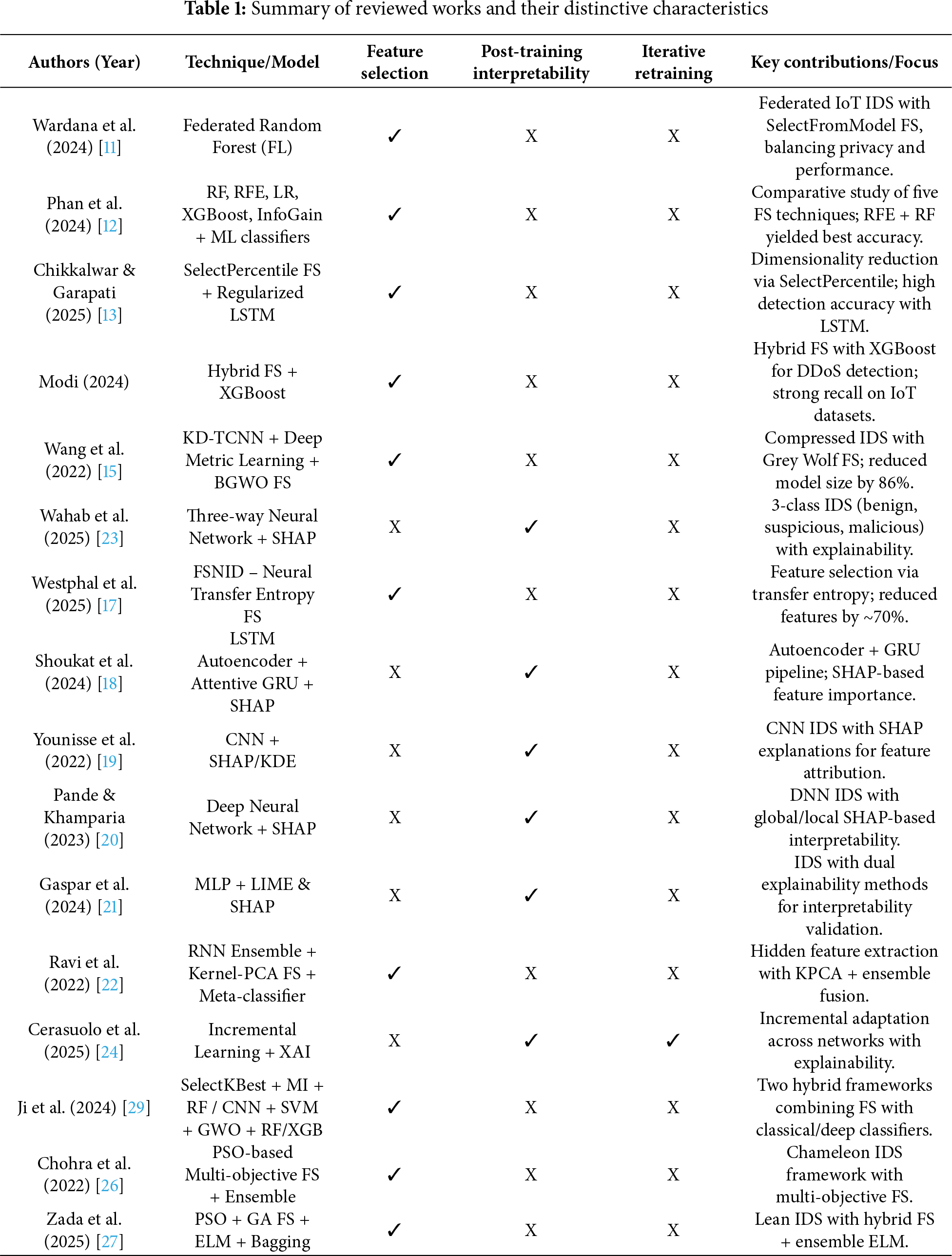
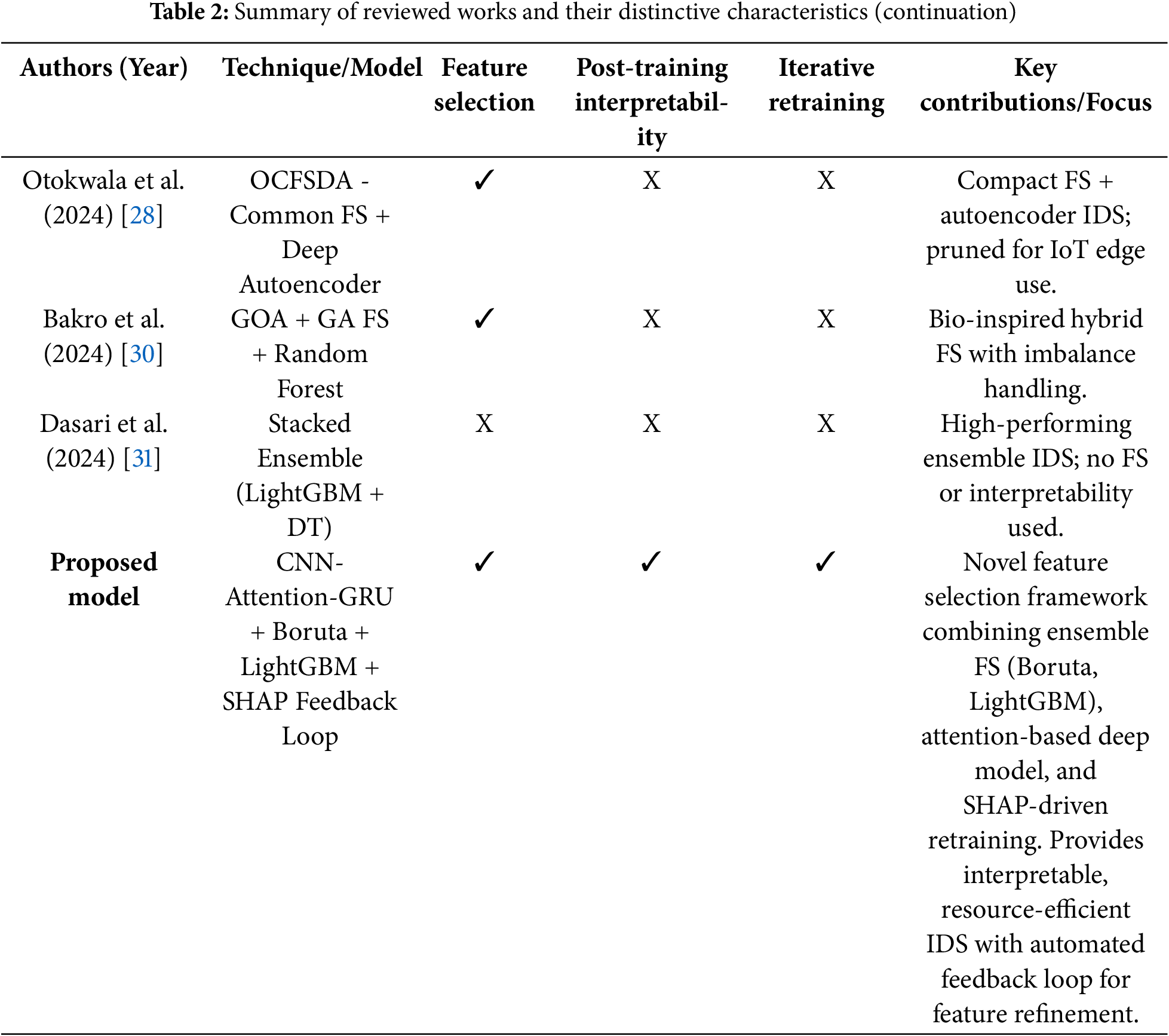
Hybrid models emerged to bridge the gap between traditional ML interpretability and deep learning performance, combining statistical measures with neural relevance tracking. More recently, ensemble-based feature selection strategies have gained popularity due to their ability to aggregate the strengths of multiple techniques, improving robustness and reducing model bias. These methods are particularly useful when working with noisy, high-dimensional datasets, such as those encountered in intrusion detection. In [25], Ji et al. proposed a hybrid feature selection method for intrusion detection in cyber-physical systems that combined bagging (Random Forest) and boosting (AdaBoost) ensembles to rank and select features based on aggregated importance scores. Using the CIC IoT 2023 dataset, the authors demonstrated that selecting the top 21 out of 46 features significantly reduced computational cost while achieving high performance metrics, including 98.27% accuracy. In [26], Chohra et al. introduced Chameleon, a hybrid feature selection framework that integrates particle swarm optimization (PSO) with ensemble classifiers to enhance network anomaly detection using deep learning autoencoders. They validated their approach on three datasets, NSL-KDD and UNSW-NB15 and IoT-Zeek yielding up to 97.302% on them, showcasing the effectiveness of PSO-guided feature selection. In [27], Zada et al. proposed a lean-based hybrid Intrusion Detection System (IDS) for IoT environments that integrates Particle Swarm Optimization (PSO) and Genetic Algorithm (GA) for feature selection, paired with Extreme Learning Machine and Bootstrap Aggregation (ELM-BA) for classification. Leveraging the CICIDS-2017 dataset, they achieved perfect detection accuracy for multiple critical attack types. In [28], Otokwala et al. introduced a hybrid feature selection framework called OCFSDA, optimized common features selection and deep-autoencoder, for lightweight intrusion detection in IoT environments. The method integrates statistical filtering with deep learning-based dimensionality reduction, yielding a compact model optimized for edge devices. Evaluated on the MQTT-IoT-IDS2020 and CIC-IDS2017 datasets, the system demonstrated strong performance with classification accuracies of 99% and 97% and ultra-low memory usage (2 KB). However, the model’s generalizability across diverse IoT contexts and resilience to adversarial manipulation remain underexplored. In [29], Ji et al. introduced two hybrid-enhanced intrusion detection frameworks, SelectKBest-MI and CNN-SVM-GWO using the CICIDS2017 and CIC IoT 2023 datasets. The first framework fused SelectKBest and mutual information filter techniques, while the second combined CNN-based extraction with SVM and Gray Wolf Optimizer for selection, leveraging both Random Forest and XGBoost classifiers for intrusion detection. They achieved 99.99% accuracy on CICIDS2017 and 99.60% accuracy on the CIC IoT 2023. In [30], Bakro et al. proposed a cloud-based intrusion detection system leveraging a hybrid feature selection approach that combines Grasshopper Optimization Algorithm (GOA) and Genetic Algorithm (GA), integrated with a Random Forest classifier for optimal performance, achieving classification accuracies of 98% on UNSW-NB15, 99% on CIC-DDoS2019, and 92% on CIC Bell DNS EXF 2021, showcasing strong multi-class and individual class performance. Finally, in [31], Dasari et al. introduced IDSELSE, a stacked ensemble learning-based intrusion detection model that employs Boruta for feature selection and combines LightGBM and Decision Tree classifiers with Logistic Regression as the meta-model, but no deep learning layer has been used. Tables 1 and 2 summarize the reviewed literature.

3  Dataset

The CIC IoT 2023 dataset [32] was chosen for this work, which is a comprehensive intrusion detection dataset tailored specifically for modern IoT (Internet of Things) environments. What makes this dataset unique is the level of effort put into replicating a real-world smart environment using actual hardware rather than simulations. The researchers behind the dataset constructed a physical lab setup mimicking a smart home and smart city ecosystem by integrating a wide range of devices such as smart TVs, thermostats, speakers, sensors, and even surveillance systems. These devices were configured to communicate using typical IoT protocols over both wired and wireless networks, just like what we see in real deployments.

To make the dataset truly representative of today’s cyber threat landscape, the creators generated a mix of legitimate and malicious network traffic. For the attack scenarios, they launched over 30 different types of intrusions, including well-known categories like Distributed Denial of Service (DDoS), brute force attacks, spoofing, reconnaissance, web-based exploits, and even malware behaviors like backdoors and botnet communication. This was done using various attack tools and scripts to emulate how actual cybercriminals target vulnerable devices. One particularly important strength of this dataset is that it combines both the diversity and volume of attacks, which helps in building robust machine learning models. From a data collection standpoint, they used powerful traffic capturing tools like Wireshark and tcpdump and then extracted meaningful flow-based features. Each network flow is represented with more than 40 carefully engineered features, such as packet counts, flag statistics, inter-arrival times, protocol types, and durations. These features reflect both low-level TCP/IP behaviors and high-level application patterns, making them extremely useful for learning attack patterns in supervised models.

The reason for selecting this dataset for our feature selection-based deep learning model is twofold. First, the dataset is compatible with deep learning architectures designed for tabular data due to the way it was generated and preprocessed. According to the authors of the dataset, network traffic was first captured at the packet level and then several features were extracted using the DPKT package, which were then stored in separate csv files. They also removed the timestamp from the list since it did not illustrate the network behavior [32]. Each row in the dataset corresponds to an independent network flow, summarized into statistical descriptors including inter-arrival time, packet size statistics (minimum, maximum, average, variance), protocol flag counts, and byte totals. This transformation removes raw sequential packet dependencies, producing a fixed-length feature vector for every flow. As a result, the dataset lacks explicit temporal or spatial dependencies across samples. Flows are not ordered, nor do they directly influence one another, and there is also no need for techniques such as sliding windows. Second, the dataset’s scale and variety, in terms of both benign and attack classes, provides a realistic and challenging ground for building generalizable models that can perform well on unseen traffic types. Its richness in both balanced and imbalanced classes gives way to test advanced techniques like SMOTE, focal loss, and SHAP interpretability under realistic conditions.

3.1 Dataset Preparation and Preprocessing

With a total of 46,686,579 samples, the CIC IoT 2023 dataset captures flows from various real-world attack vectors including DDoS, DoS, Mirai, Brute Force, Spoofing, and Web-based attacks. Given the computational and memory constraints typically associated with training deep learning models, it was neither feasible nor necessary to train on the entire dataset. Therefore, approximately 18.5 million samples, roughly 40% of the total, were selected for training and evaluation purposes. This selection strategy ensured diversity while maintaining practical training times.

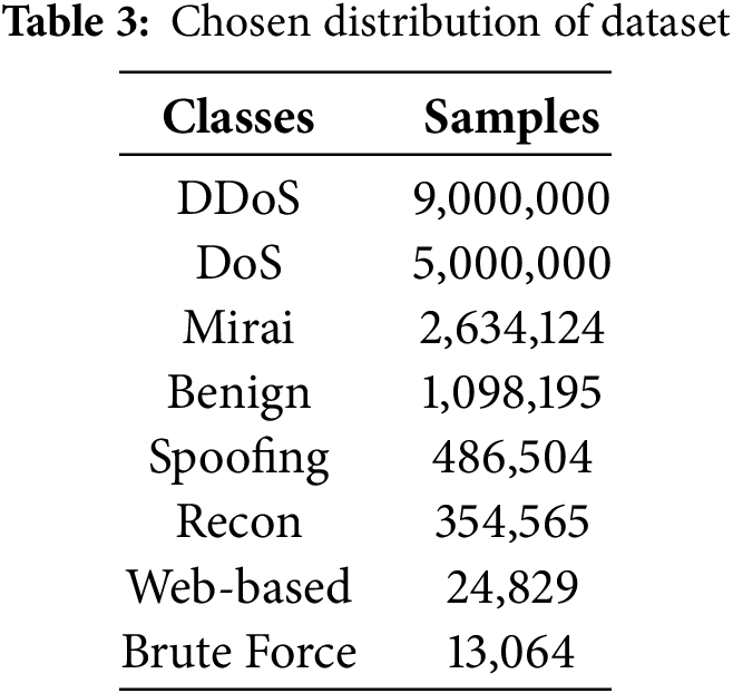
The dataset labels were then mapped into 8 consolidated classes, grouping multiple sub-attack types under broader categories (e.g., all types of DDoS attacks were grouped under a single “DDoS” class). This consolidation made the classification task more robust and interpretable, while also helping balance the granularity of detection with the dataset’s inherent skew. To maximize the representation of underrepresented behaviors, all available samples from the minority classes (Brute Force, Web-based, Recon, Spoofing, Mirai and Benign) were included entirely. These classes each had relatively small sample sizes, making them suitable for full inclusion without the risk of overwhelming the dataset. For the major classes, DDoS and DoS, the dataset was randomly undersampled to ensure they did not dominate the model’s learning process. The final class-wise sample distribution prior to splitting is shown in Table 3.

Following the data selection, the 46 original features were then filtered using a two-stage feature selection strategy: first, Boruta was applied to eliminate statistically irrelevant and redundant features, and then LightGBM with SHAP values was used to rank and refine the remaining features based on their importance to the prediction task. This process reduced the number of features to 30 highly relevant ones, removing unnecessary noise and improving model interpretability. Finally, a StandardScaler was used to normalize the data such that each feature had zero mean and unit variance. This step is crucial in neural network training to ensure faster convergence and to prevent the optimizer from getting stuck in suboptimal local minima due to disproportionately scaled input features. After scaling, the dataset was shuffled to eliminate any unintended ordering that might bias the model, especially since flows from the same attack type could have been logged in contiguous blocks during collection.

3.2 Dataset Splitting and Rebalancing

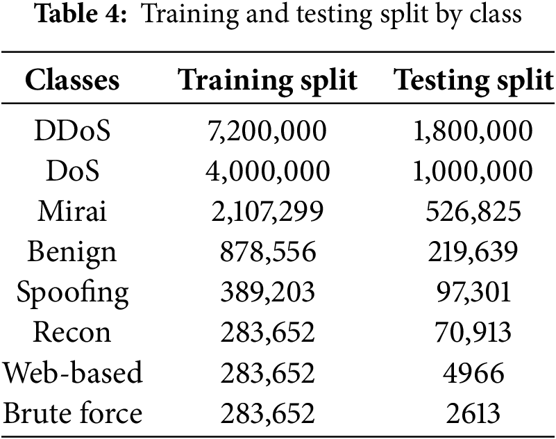
After preprocessing, the cleaned and scaled dataset was split into training and testing sets using an 80:20 stratified split. Stratification was necessary to maintain the original class proportions in both subsets, which is critical when dealing with highly imbalanced data. The training class distribution remained heavily skewed after the initial split, with dominant classes such as DDoS and DoS vastly outnumbering minority classes like Brute Force and Web-based attacks. To mitigate this issue, SMOTE (Synthetic Minority Over-sampling Technique) was used to generate synthetic samples inside the training split, specifically for the two most underrepresented classes (Brute Force and Web-based), until they reached parity with the third smallest class (Recon). This selective balancing approach allowed for better learning on rare attack types without disturbing the natural class distribution of the more representative classes. The final training and testing distributions are shown in Table 4.

Instead of forcing all classes to have identical sample sizes, which might introduce synthetic bias or overfitting, the rebalancing was designed to elevate only the smallest classes to a reasonable threshold. This retained the integrity of naturally frequent classes like DDoS and DoS while preventing the minority classes from being ignored during training. The random shuffle applied afterward ensured that all training data was well-distributed, further aiding generalization during the learning phase.

4  Design and Modeling of the Proposed Feature Selector

Given the high dimensionality and potential noise present in tabular intrusion detection datasets, a careful feature selection strategy was critical to improve model efficiency and interpretability. To that end, two complementary approaches were applied prior to training the deep learning model: Boruta and LightGBM with SHAP. These techniques were chosen not only for their ability to reduce dimensionality but also for their effectiveness in uncovering relevant relationships in non-linear and imbalanced data environments.

4.1 Boruta

Boruta was used as an all-relevant feature selection method, built on top of the Random Forest classifier. The method works by creating “shadow features”, shuffled versions of the original features that serve as noise benchmarks. A Random Forest is trained using both original and shadow features, and each real feature is then compared to the best-performing shadow feature. If a feature significantly outperforms its noisy counterpart based on Z-score statistics, it is retained. This comparison process is repeated iteratively, eliminating irrelevant features at each round until only confirmed or rejected features remain. Boruta is especially well-suited for intrusion detection datasets, which often contain redundant features such as Rate and Srate, or flags with overlapping meanings. By not arbitrarily favoring only the strongest signals, Boruta ensures that all relevant, but potentially subtle, features are preserved. Its robustness against noise and ability to capture non-linear interactions make it ideal for scenarios where patterns like syn_flag_number interacting with Rate play a key role in identifying attack types such as SYN floods.

The derivation below outlines the core mathematical principles used by Boruta to score and validate features [33]. Let xt∈Rn denote the vector of n input features for the t-th sample, and let yt∈R be the corresponding target value, where t=1,2,…,T for a total of T instances. For every original feature vector xt, a randomly shuffled duplicate (called a shadow feature) is created, denoted as xt′. To determine the relevance of a feature, its Mean Decrease in Accuracy (MDA) is computed by comparing the model’s prediction performance when using the original feature vs. its shuffled (shadow) version as given in Eq. (1) [34].

MDA=1mtree∑m=1mtree∑t∈OOBI(yt=f(xt))∑t∈OOBI(yt=f(xt′))|OOB|(1)

where mtree is the total number of trees (e.g., 500), I(⋅) is the indicator function: I(A)=1 if A is true, and 0 otherwise, while OOB refers to the Out-of-Bag samples (those excluded from training the m-th tree), f(⋅) is the prediction function of the trained model.

This measures how much prediction accuracy drops on OOB samples when the real feature is replaced by its permuted counterpart. Next, to normalize the importance of each feature, the Z-score is calculated using the standard deviation of MDA values across all trees as in Eq. (2).

Z-score=MDASD(2)

where SD is the standard deviation of the accuracy losses (MDAs) across trees. Furthermore, a decision rule for feature selection is applied where each feature is compared to the shadow features based on its Z-score. A feature is:

Confirmed important if Z-score>Zmax,

Rejected (or unimportant) if Z-score<Zmax,

where Zmax is the highest Z-score among all shadow (randomized) features.

4.2 LightGBM + SHAP

Complementing Boruta, LightGBM combined with SHAP (SHapley Additive Explanations) was also employed. LightGBM is a fast, high-performance gradient boosting framework that is particularly adept at handling high-dimensional, sparse, and imbalanced datasets, common characteristics in network intrusion data. Once a LightGBM model was trained on the preselected features, SHAP values were computed to assign a unique importance score to every feature for each prediction. These SHAP scores are grounded in cooperative game theory, measuring how much each feature contributes to the model’s prediction relative to a baseline expectation. By averaging the absolute SHAP values across all samples, a global ranking of feature importance was obtained. This ranking helped identify which features had the most influence on the model’s decision-making process, for instance, highlighting that high values of Rate were strongly associated with DDoS attacks, or that syn_flag_number was only impactful when TCP was enabled.

LightGBM’s roots can be traced back to Gradient Boosting Decision Trees (GBDT), which laid the foundation for many tree-based ensemble methods, and were the starting point for SHAP explainability, which was later adapted for XGBoost and then LightGBM. In its core form, the forward additive model is defined as Eq. (2) [35]

f(x)=∑i=1Mβih(x;θi)(3)

where x is an input feature vector and h(x;θi) denotes the i-th base learner. The overall model is constructed as a sum of M such learners weighted by βi. The objective is to minimize the loss over N training instances using

minf∑j=1NL(f(xj),yj)=minf∑j=1NL(∑i=1Mβih(xj;θi),yj)(4)

where (xj,yj)j=1N is the dataset and the model is constructed incrementally. The negative gradient of the loss with respect to each sample prediction is computed as in Eq. (5) and the goal is to find h(xj;θM) and βM that best fit this residual in a least-squares sense as given in Eq. (6)

gj=−∂L(fM−1(xj),yj)∂fM−1(xj)(5)

θM,βM=arg⁡minθ,β∑j=1N|gj−βh(xj;θ)|2(6)

After identifying the best-fitting function, the optimal step size ρM is then determined via:

ρM=arg⁡minρ∑j=1NL(fM−1(xj)+ρh(xj),yj),(7)

resulting in the updated model

f(x)=fM−1+ρMβMh(x;θM)(8)

While effective, traditional GBDT is susceptible to overfitting and can be computationally expensive due to the need to scan all feature values for split selection. XGBoost improved on this by introducing regularization and a second-order Taylor approximation, requiring both gradients and Hessians (xj,gj,hj)j=1N, and uses Eq. (9) for calculating split gain, while computing the leaf value using Eq. (10)

Gain=12[GL2HL+λ+GR2HR+λ−(GL+GR)2HL+HR+λ]−γ,(9)

Wj=−GjHj+λ(10)

where GL and HL are the gradient and Hessian sums for the left node, and GR, HR are for the right. Wj is the weight for leaf j, and λ, γ are regularization terms. XGBoost struggled with large datasets due to high memory and training demands. LightGBM was proposed to address these scalability issues and extend the utility of SHAP explainability to larger problems [36]. It improves performance by growing trees leaf-wise (rather than level-wise) and introducing histogram-based decision trees, which bucket continuous values to reduce memory and speed up training. Furthermore, it leverages Gradient-based One-Side Sampling (GOSS) to focus on instances with large gradients and implements several parallelism strategies. The training cost of each tree node split is defined as:

costtime=featurenum×samplenum×pointnum(11)

where featurenum is the number of input features, samplenum the training instances, and pointnum the number of candidate splits. LightGBM’s ability to natively handle categorical features, its efficient histogram and sampling strategies, and cache-aware memory access have made it one of the most powerful and scalable implementations of GBDT, allowing it to be paired effectively with SHAP for reliable feature importance estimation in large-scale intrusion detection tasks.

4.3 The Proposed Ensemble of Feature Selection

To address the high dimensionality and redundancy inherent in intrusion detection datasets, we propose a mathematically grounded hybrid feature selection ensemble that combines the statistical robustness of Boruta with the fine-grained interpretability of LightGBM + SHAP. As shown in Fig. 1, Boruta, as an all-relevant selector, prunes the dataset by removing noisy or redundant traffic features in a statistically reliable way while preserving all potentially important features. Since it builds on Random Forest, it is more robust than plain tree-based rankings and avoids bias toward high-cardinality features. LightGBM + SHAP then adds a complementary stage, providing clear, interpretable explanations of feature importance—without reducing features into hard-to-interpret components as in PCA or relying solely on linear assumptions as in mutual information. This two-step approach is still underexplored in IDS research, and we chose it specifically to provide both novelty and stronger interpretability compared to conventional single method feature selection. Exactly 10,000 samples were taken from all 8 classes and after applying the ensemble, the results consisted of a concise, well-informed set of features that balanced interpretability, predictive power, and robustness against overfitting, setting a solid foundation for the subsequent deep learning model. In the end, 30 out of 46 features were selected to be sent to the next phase. Once the model is trained, an explainability tool will be used to assess the key predictive features, and those features can be saved and used to retrain the existing model or develop a new model. The 30 selected features on which the model was trained on are discussed in Section 7.6.

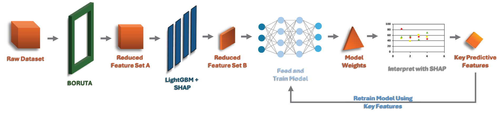
Figure 1: The proposed AutoSHARC pipeline for feature selection with SHAP-guided retraining

The two-stage feature selector is formulated to identify all relevant features (strong and weak) and then re-rank them based on their contribution to predictive performance. Let the original dataset be denoted by 𝒟={(x(i),y(i))}i=1N, where x(i)∈Rd is the i-th feature vector with d dimensions, and y(i) is its corresponding label.

4.3.1 Stage 1: Boruta Pruning via Shadow Features

The Boruta algorithm first augments 𝒟 by generating permuted “shadow” features x′(i) for each original feature:

𝒟′={(x(i)‖x′(i),y(i))}i=1N,(12)

where ∥ denotes feature-wise concatenation. A random forest classifier is trained on 𝒟′ to compute importance scores ℐj for each feature xj based on the Mean Decrease in Accuracy (MDA):

ℐj=1T∑t=1T1|OOBt|∑i∈OOBt[I(y(i)=ft(x(i)))−I(y(i)=ft(x[j←perm](i)))],(13)

where T is the number of trees, OOBt denotes out-of-bag samples for tree t, and ft is the prediction of the t-th tree. Feature j is retained if its average Z-score across trees satisfies:

Zj=ℐj−μshadowσshadow>maxkZkshadow,(14)

where μshadow and σshadow are the mean and standard deviation of shadow feature importances.

Let ℱboruta⊂{1,2,...,d} denote the set of features retained after Boruta.

4.3.2 Stage 2: SHAP-Based Ranking via LightGBM

Using the reduced feature set ℱboruta, a LightGBM model is trained and Shapley values ϕj(i) are computed for each feature j∈ℱboruta for each instance i:

f(x(i))=ϕ0+∑j∈ℱborutaϕj(i),(15)

where ϕ0 is the expected model output over the dataset. The global importance of each feature is quantified by the mean absolute Shapley value:

Φj=1N∑i=1N|ϕj(i)|,j∈ℱboruta.(16)

Features are then ranked in descending order of Φj, and the top-k features are selected:

ℱselected=Topk⁡({Φj∣j∈ℱboruta}),(17)

with k=30 determined empirically to balance model accuracy and dimensionality.

Thus, the complete feature selection operator 𝒮 can be expressed as the composite function:

ℱselected=𝒮(𝒟)=ℛSHAP∘ℬBoruta(𝒟),(18)

where ℬBoruta denotes the Boruta filter and ℛSHAP denotes the LightGBM+SHAP ranker.

This selected feature set ℱselected is then forwarded to the deep learning classifier for training. The full AutoSHARC pipeline (see Fig. 1) thus leverages this mathematical design to ensure relevance, interpretability, and performance in high-dimensional intrusion detection.

5  The Proposed Model for Intrusion Detection

The intrusion detection model designed for the CIC IoT 2023 dataset is a hybrid deep learning architecture that combines 1D Convolutional Neural Networks (CNNs), an attention mechanism, a Gated Recurrent Unit (GRU), and a final dense output layer. Unlike traditional models that focus purely on classification performance, this model is specifically designed with feature selection as a primary objective. The goal is not only to predict attack types accurately but also to identify and isolate the most important input features contributing to each decision.

5.1 Architectural Components of the Proposed Model

5.1.1 CNN Layer—Local Feature Transformation

Despite the absence of natural spatial or temporal structure in the dataset, a 1D CNN is used as the first layer. In traditional settings, CNNs are applied to image data to detect spatial patterns. However, in this architecture, the Conv1D layer acts more like a nonlinear feature extractor. Applying a 1D convolution helps capture local patterns or relationships among neighboring features in each sample. It scans the input feature vector with a small kernel, capturing local groupings or interactions between adjacent features. Although the features in the CIC IoT 2023 dataset are not ordered in time or space, it is still plausible that certain adjacent or co-occurring features (e.g., packet size and packet rate) interact meaningfully when viewed together.

The real value of CNN here lies in its ability to transform the input into a richer latent representation through parameter sharing and local filtering. It’s a computationally efficient way to project the raw input features into a new space, preparing them for more expressive attention and recurrent layers. Importantly, the CNN does not assume or enforce spatial continuity. It just helps extract compact, meaningful representations at the feature level.

A 1D Convolutional Neural Network (1D-CNN) processes sequential data by extracting local patterns using convolution and pooling operations. In each convolutional layer, a feature map Zm is computed using a sliding window across input sequences, where each output element zm,r is derived from localized filters [37]. Mathematically, the output of the rth unit in the mth feature is calculated as:

zm,r=ϕ(∑u=1U∑v=1Vau,v+r−1⋅Ku,m,v+bm),(19)

where ϕ denotes the activation function, au,v represents the vth element of the uth input sequence, Ku,m,v is the filter kernel linking the uth input to the mth output map, and bm is a trainable bias term. The convolutional process can also be compactly expressed as:

Zm=ϕ(∑u=1UAu∗Kum),(m=1,2,...,M),(20)

where ∗ indicates the convolution operator. Once local features are extracted, a pooling layer reduces dimensionality and emphasizes dominant activations. In the case of max pooling, the rth output from the mth feature map is computed as:

ρm,r=maxn=1N(zm,(r−1)⋅δ+n),(21)

where N is the pooling window size and δ is the stride. Alternatively, in average pooling, the output is calculated using:

ρm,r=η∑n=1N(zm,(r−1)⋅δ+n),(22)

with η representing the scaling factor. While both methods reduce spatial dimensions, max pooling typically captures more prominent features [38] and is therefore chosen.

5.1.2 Attention Layer—Feature Selection by Design

Following the CNN, an attention mechanism, specifically a custom single-headed, non self-attention layer, is applied. This layer is designed to assign importance scores to each extracted feature, thereby functioning as an explicit feature selector. This approach aligns with the core motivation for designing the model: to select and prioritize the most informative features in a highly interpretable way. Importantly, unlike other attention mechanisms such as self-attention or transformer blocks, this attention layer does not assume any sequential or spatial dependencies in the data. In intrusion detection datasets like the one used here, each row is independent, and the features typically do not follow a temporal or spatial structure. Hence, complex attention models that calculate pairwise dependencies or rely on positional encodings would not only be computationally excessive but might also lead to overfitting by modeling noise instead of signal. Instead, this simple attention gate provides a targeted and computationally efficient way to weight each feature’s contribution, ensuring relevance-driven learning without architectural overkill.

The derivation below formalizes the operation of the attention-based feature selection layer used in our model, which implements a per-feature gating mechanism [39]. Let x∈RT denote the input feature vector for a single instance, where T is the number of time steps or features. The attention mechanism computes a scalar importance score for each feature xi, where i∈{1,2,…,T}, and uses it to reweight the input feature. This process begins with the application of a trainable dense layer (with shared weights across all features), which applies a linear transformation to each feature value xi using a weight W and bias b, as shown in Eq. (16):

si=Wxi+b(23)

This raw score si is passed through a sigmoid activation function σ(⋅) to produce an attention coefficient αi∈(0,1), as expressed in Eq. (17):

αi=σ(si)=11+e−si=11+e−(Wxi+b)(24)

The sigmoid output acts as a gating value that determines the relevance of the corresponding input feature xi, where αi close to 1 retains the feature and αi close to 0 suppresses it [40]. The original input feature is then reweighted in Eq. (18) using this coefficient to produce the gated output yi as follows:

yi=αi⋅xi=σ(Wxi+b)⋅xi(25)

To represent this mechanism compactly over the entire feature vector x=[x1,x2,…,xT]T, we define α=σ(Wx+b) and express the final output as element-wise multiplication as Eq. (19)

y=α⊙x(26)

Here, ⊙ denotes the Hadamard (element-wise) product. The result is a refined feature vector y∈RT where each input component has been scaled based on its learned importance. Importantly, since the attention coefficients are computed independently for each feature and the operation does not change the feature dimensionality, the output retains the same shape as the input. This allows the attention mechanism to act as a lightweight and interpretable feature selector that enhances important features while suppressing irrelevant or noisy inputs. Such a gating mechanism is widely used in neural architectures for both interpretability and improved performance, and aligns closely with attention-based modules found in computer vision and natural language processing.

5.1.3 GRU Layer—Abstract Representation, Not Temporal Memory

Although the data lacks temporal dependencies across rows, a GRU (Gated Recurrent Unit) layer is used after the attention mechanism to introduce a form of redundancy filtering. Rather than modeling sequences over time, the GRU in this context is utilized as a gating mechanism to suppress irrelevant or redundant feature activations that might persist even after attention. The recurrent unit acts like a secondary filter, allowing the model to remember the most salient patterns selected by the attention layer and ignore fluctuations or noise that don’t consistently contribute to class discrimination. Even though there’s no real sequence, this use of GRU reflects an architectural choice for its gating capabilities, not its temporal modeling strengths.

The update gate, shown in Eq. (20), controls the extent to which the model should preserve information from the previous hidden state when processing the current input. It is calculated by applying a sigmoid activation to the linear transformation of the concatenated previous hidden state ht−1 and the current input xt [41]:

zt=σ(Wz[ht−1,xt]+bz)(27)

In a similar fashion, the reset gate in Eq. (21) governs how much of the past memory should be ignored or reset before computing the new memory candidate. It uses the same combination of ht−1 and xt and passes it through a sigmoid-activated linear layer:

rt=σ(Wr[ht−1,xt]+br)(28)

The candidate hidden state h~t is then computed using the element-wise product of the reset gate and the previous hidden state. This modified hidden state is concatenated with the current input and passed through a tanh activation, as shown in Eq. (22). This operation determines the new content to be potentially added to the memory:

h~t=tanh⁡(Wh[rt⋅ht−1,xt])(29)

Next, the new hidden state ht is formed by interpolating between the previous hidden state ht−1 and the newly computed candidate activation h~t. The mixing proportion is governed by the update gate zt, as shown in Eq. (23):

ht=(1−zt)ht−1+zth~t(30)

Optionally, an output gate ot can be used to regulate how much of the hidden state should contribute to the actual output at the current time step. This is done in Eq. (24) by applying another sigmoid function to the affine transformation of ht:

ot=σo(Woht+bo)(31)

Here, Wo and bo represent the trainable weights and biases of the output transformation layer, respectively. Together, these equations form the backbone of the Gated Recurrent Unit (GRU), which balances information retention and update through learned gating mechanisms.

5.1.4 Dense Output Layer—Multiclass Classification

After extracting and aggregating features through the CNN, attention, and GRU layers, the model outputs a prediction through a fully connected dense layer with a softmax activation function. This standard setup produces a probability distribution over the target classes (e.g., DDoS, Mirai, Web-based, etc.). The use of softmax ensures that predictions are interpretable and that the model’s confidence in each class can be quantified. This is especially useful for downstream evaluation metrics like ROC-AUC, precision-recall, and for interpretability tools like SHAP. Since class imbalance is a known challenge in cybersecurity datasets, this final stage benefits from the refined and focused input features produced by the earlier layers, helping the classifier make more informed predictions with reduced overfitting risk.

5.2 Architectural Details of the Proposed Model

The overall design of the model is intentionally built around the concept of intelligent feature selection rather than complex sequential modeling. The dataset is tabular, 1D, and likely does not exhibit spatial or temporal dependencies, each sample is an independent observation of network activity. Therefore, applying sequence-heavy architectures like RNNs or transformers would be inefficient and prone to overfitting. Fig. 2 shows that the CNN layer provides a simple but effective form of feature preprocessing. The attention mechanism offers interpretability and focused learning without the overhead of self-attention. The GRU acts more as a content filter than a sequence model. Combined, these layers form a lightweight yet powerful pipeline for handling imbalanced, high-dimensional intrusion detection data while prioritizing clarity, performance, and resource efficiency.

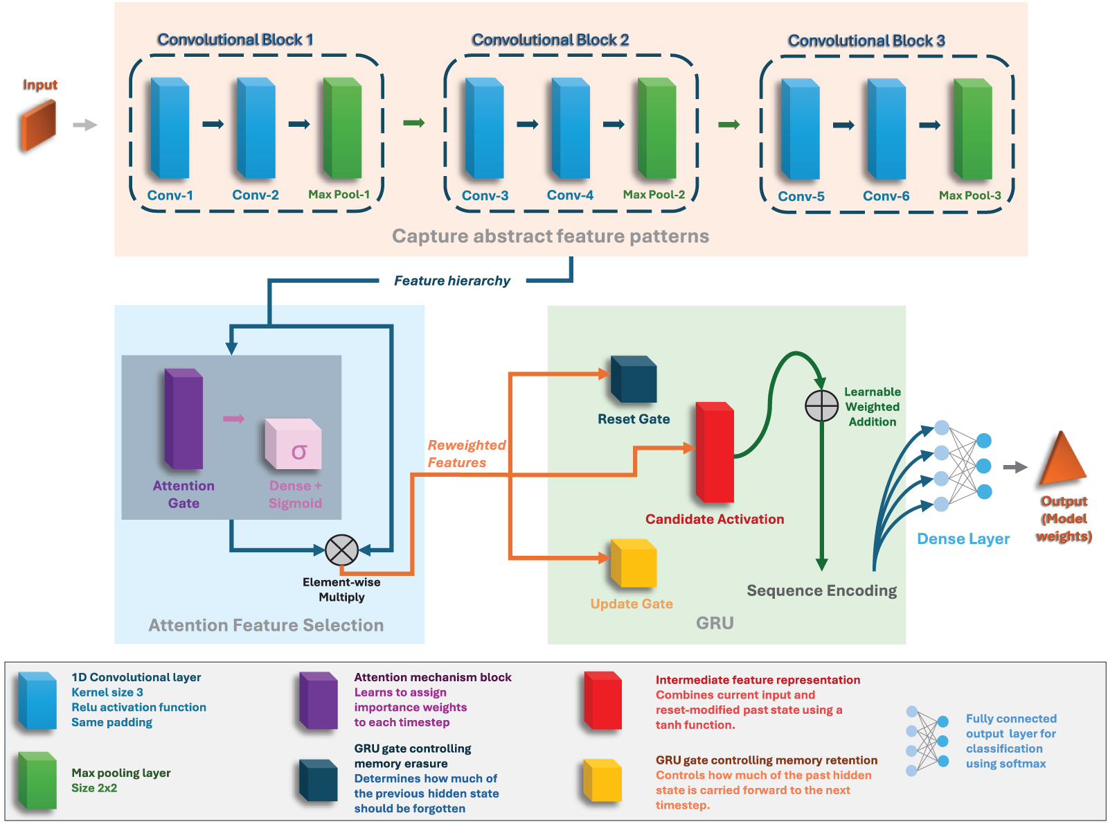
Figure 2: The proposed model architecture

The proposed deep learning model is designed as a structured feature refinement pipeline, where each component contributes to progressive filtering, transformation, and selection of the most discriminative features for intrusion detection. Given a preprocessed input vector x∈RT, where T=30 features selected by the ensemble mechanism, the model transforms x through three core stages: convolutional embedding, attention-guided feature selection, and gated refinement.

5.2.1 Stage 1: 1D Convolutional Feature Transformation

The input is reshaped as x∈RT×1 and passed through L stacked 1D convolutional layers, each applying Mℓ kernels of width wℓ. For layer ℓ, the convolutional transformation is given by:

Z(ℓ)=ReLU(W(ℓ)∗Z(ℓ−1)+b(ℓ)),ℓ=1,2,…,L,(32)

where ∗ denotes 1D convolution, W(ℓ) are trainable filters, b(ℓ) biases, and Z(0)=x. This transformation captures low-level local interactions between adjacent features, such as packet rate and packet size.

5.2.2 Stage 2: Attention-Based Feature Selection

Following convolution, the output Z∈RT′×d is reweighted using a learned feature-wise attention vector α∈[0,1]T′, where each element αi is computed as:

αi=σ(w⊤zi+b),i=1,…,T′,(33)

where zi∈Rd is the i-th feature vector after CNN, σ(⋅) is the sigmoid function, and (w,b) are shared attention parameters. The reweighted representation becomes:

z~i=αi⋅zi,andZ~=[z~1,z~2,…,z~T′].(34)

This operation acts as a soft feature selector, enhancing informative feature maps and suppressing noisy or redundant ones.

5.2.3 Stage 3: Gated Refinement via GRU

Although the data is non-sequential, we leverage the **gating mechanism** of GRUs to selectively propagate stable feature activations. The GRU operates over the feature dimension rather than time:

zt=σ(Wzzt+Uzht−1+bz),(35)

rt=σ(Wrzt+Urht−1+br),(36)

h~t=tanh⁡(Whzt+Uh(rt⊙ht−1)+bh),(37)

ht=(1−zt)⊙ht−1+zt⊙h~t,(38)

where ⊙ is the element-wise product. The final GRU hidden state hT serves as the abstract, filtered feature embedding for classification.

5.2.4 Training Dynamics: Optimization and Loss Function

In the training phase, the model was initially optimized using the RMSprop optimizer in conjunction with focal loss. This pairing was specifically chosen to handle severe class imbalance and to give greater attention to hard-to-classify minority samples. RMSprop proved effective at stabilizing learning in the earlier epochs. For fine-tuning, the optimizer was switched to Adam while retaining focal loss with greater alpha values for the minority classes. This change allowed for more adaptive learning rates across parameters, accelerating convergence and refining performance once the model had achieved a stable baseline. The consistent use of focal loss throughout both phases ensured that minority class recall and robustness remained a central focus in the optimization strategy.

RMSprop

RMSprop is a popular method for training deep learning models using adaptive learning rates [42]. Let xt∈Rd denote the parameter vector at iteration t, and let gt=∇f(xt) represent the stochastic gradient computed at that step. The goal is to minimize a possibly non-convex stochastic objective function of the form of Eq. (25) [43]:

f(x)=Eξ∼P[f~(x,ξ)],(39)

where ξ is a random variable sampled from an unknown distribution P, and f~(x,ξ) denotes the stochastic loss for a given input ξ. To address the instability that may arise from the varying magnitude of gradients across coordinates, RMSprop maintains an exponential moving average of the squared gradients, allowing the learning rate to adaptively scale for each parameter. Formally, for each coordinate k∈{1,2,…,d}, the update rules in Eqs. (26) and (27) define RMSprop:

vt,k=θtvt−1,k+(1−θt)gt,k2,(40)

xt+1,k=xt,k−αtgt,kvt,k+ϵ,(41)

where θt∈(0,1) is the decay factor controlling the memory of past squared gradients, αt is the base learning rate at time t, and ϵ>0 is a small constant for numerical stability. To express RMSprop as a special case of an adaptive gradient method, we can interpret the denominator as a normalization term that adjusts the effective learning rate as Eq. (28) which implies a coordinate-wise gradient descent update in Eq. (29)

ηt,k=αtvt,k+ϵ,(42)

xt+1,k=xt,k−ηt,kgt,k.(43)

This mechanism allows RMSprop to take larger steps in directions where gradients have historically been small, and smaller steps in directions where gradients have been consistently large. In practice, θt is often held constant (e.g., θt=0.9 or 0.99), and the base learning rate αt is typically set as a small fixed value. RMSprop is widely used due to its simplicity and robustness in handling non-stationary objectives and sparse gradients. However, care must be taken in selecting the hyperparameters, particularly θt and αt, to ensure proper convergence behavior [44]. RMSprop provides early stability, while Adam improves convergence via momentum and adaptive learning rates.

Focal Loss for Class Imbalance

To address class imbalance, we employ focal loss, which emphasizes hard-to-classify samples:

ℒfocal=−∑i=1Cαi(1−pi)γyilog⁡(pi),(44)

where C is the number of classes, yi is the true label (one-hot), pi is the predicted probability, αi is the class-specific weight, and γ controls focus on difficult examples. Given a classification task with C classes, let y=(y1,y2,…,yC) be the one-hot encoded ground truth label and p=(p1,p2,…,pC) be the predicted probabilities (output of softmax). The cross-entropy loss is given by Eq. (30) [45]

ℒCE(y,p)=−∑i=1Cyilog⁡(pi)(45)

Since y is one-hot encoded, only the true class index t has yt=1, and all others are 0. Therefore,

ℒCE=−log⁡(pt)(46)

To handle class imbalance, a weighting factor α∈(0,1] is introduced for the true class:

ℒα=−αtlog⁡(pt)(47)

The focal loss introduces a modulating factor (1−pt)γ to focus learning on hard misclassified examples. The parameter γ≥0 controls this focus:

ℒfocal=−αt(1−pt)γlog⁡(pt)(48)

This reduces the loss contribution from easy examples (where pt is close to 1) and emphasizes harder ones. Extending the focal loss to the full multi-class case using one-hot encoding:

ℒfocal(y,p)=−∑i=1Cαi⋅(1−pi)γ⋅yilog⁡(pi)(49)

Here, yi is 1 only for the true class, 0 otherwise, pi is the predicted probability for class i, αi is the class-specific weight (same for all classes if uniform). Since only yt=1 for the true class t, the sum reduces to:

ℒfocal=−αt(1−pt)γlog⁡(pt)(50)

5.2.5 Architectural Hyperparameters

The design of the CNN-Attention-GRU model, as given in Table 5, was driven by a careful balance between performance, interpretability, and stability. The 1D Convolutional layers were chosen to effectively capture local patterns and interactions between adjacent features, which is ideal for tabular intrusion detection data where spatial proximity in features can reflect meaningful structure. Instead of deeper CNN stacks, we used shallow but wide filters to minimize overfitting while still extracting robust patterns. The GRU layer was selected over LSTM or Transformer layers due to its lower parameter count, faster convergence, and reduced risk of overfitting on tabular data without temporal dependencies. GRUs performed consistently better in experiments, offering stable learning dynamics without the complexity of LSTMs’ memory cell gates or the training instability of Transformer-based models on small datasets. The attention mechanism was integrated to enhance the model’s ability to select and focus on the most important features, acting as a soft feature selector that improves both performance and explainability. Regularization techniques like batch normalization and dropout were intentionally omitted after extensive testing, as they introduced instability in training and degraded performance rather than enhancing generalization. This was likely been due to the feature space post preprocessing and SMOTE, making such regularizations unnecessary. Predictions were assigned to the class with the maximum softmax probability (argmax). No per-class probability thresholds were optimized for this model. The batch size used was 2048 to maximize training speed. Overall, each component in the architecture was purposefully selected to maximize accuracy while maintaining interpretability and stability, with all unnecessary complexity stripped away. Thy hyperparameters used for the proposed model are given in Table 6.

5.2.6 Model Parameters

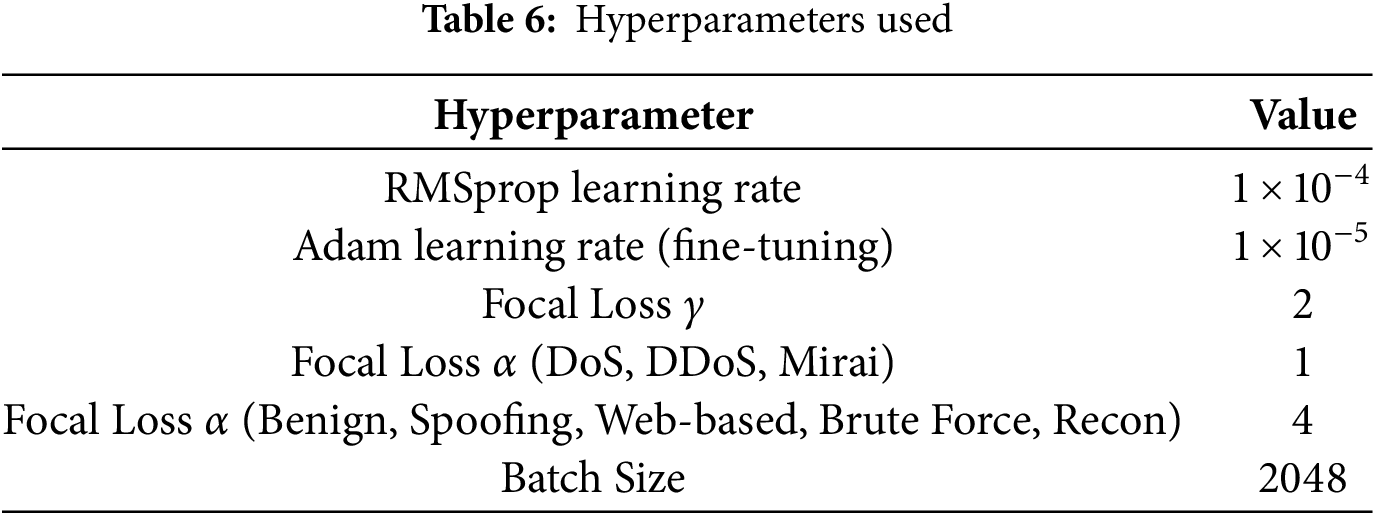
The final model consisted of approximately 531,272 trainable parameters, as displayed in Table 7, occupying only 2034 KB of storage space. This compact architecture was deliberately designed to strike a balance between performance and efficiency. One of the guiding principles in building this model was to maintain a lightweight footprint while preserving the model’s ability to learn rich feature representations. Given the nature of the dataset, where each row represents an independent sample without temporal or spatial dependencies, it was unnecessary to use deeper or heavier models that might introduce overfitting or unnecessary complexity. The choice of using a compact CNN-GRU architecture with an attention mechanism ensured that only the most relevant features were selected and passed through, allowing the network to focus on meaningful patterns without redundancy. This resulted in a model that is resource-efficient, suitable for deployment in real-world or edge environments, and fast during both training and inference, without compromising classification performance.

6  SHAP for Explainability

SHAP (SHapley Additive exPlanations) was used in this study as a post-training explainability tool to assess and interpret the contribution of each input feature to the model’s predictions. Unlike black-box models where interpretability is minimal, SHAP enables a detailed breakdown of how each feature pushes the prediction toward or away from a certain class. It offers consistent and theoretically grounded feature attributions, unlike LIME which relies on unstable local approximations, or Counterfactuals which focus only on individual “what-if” scenarios. SHAP not only explains single predictions but also provides global feature importance, making it especially suited for our dataset where flows are described by more than 40 engineered features. This makes it particularly powerful in the context of feature selection, especially when interpretability, transparency, and generalization are just as important as predictive accuracy. In our case, after applying a layered feature selection strategy during preprocessing (Boruta and SHAP + LightGBM), the application of SHAP again after training acted as a final interpretability pass, providing reassurance that the model was relying on truly relevant features during inference.

SHAP is based on cooperative game theory, assigning each feature an importance value for a particular prediction by estimating how the prediction changes when that feature is removed or added. It attributes these changes fairly across all features by considering all possible combinations. This provides local explanations (per-sample) that can be aggregated into global explanations to understand the overall behavior of the model. In a domain like intrusion detection, where model decisions can affect system-level security responses, this level of insight is critical. SHAP helps validate not only that the model is accurate but also that it is making the right decisions for the right reasons.

The SHAP approach used in this work is Kernel SHAP, a model-agnostic technique grounded in cooperative game theory. It estimates the contribution of each feature to a specific model prediction using Shapley values. Given a model f, an input sample x∈RM, and a specific feature i∈{1,2,…,M}, the SHAP value ϕi represents the marginal contribution of feature i averaged over all possible feature subsets S⊆F∖{i}, where F is the full feature set. The Shapley value is formally defined as:

ϕi(f,x)=∑S⊆F∖{i}|S|!(|F|−|S|−1)!|F|

Since computing this exactly is computationally expensive for large M, Kernel SHAP approximates the Shapley values by solving a weighted linear regression problem over perturbed binary feature masks. The SHAP values ϕ∈RM are obtained by minimizing the following objective:

ϕ=arg⁡minϕ∈RM∑z′∈Z[f(hx(z′))−ϕTz′]2πx(z′)(52)

Here, z′∈{0,1}M is a binary mask indicating which features are included, hx(z′) is the function that constructs a full input from a masked version by filling missing features with background values, and πx(z′) is the Shapley kernel which assigns a weight to each subset:

πx(z′)=M−1(M|z′|)⋅|z′|⋅(M−|z′|)(53)

In our implementation, 500 randomly selected training samples serve as the background distribution, while 50 test samples are explained. Since the model includes a custom attention layer and focal loss function, we use a prediction wrapper to reshape the input into the required 3D form, enabling compatibility with KernelExplainer. This allows the SHAP values to reliably attribute feature contributions even in the presence of a complex, non-linear neural architecture.

In our analysis (Fig. 3), we used several SHAP output formats to gain a comprehensive understanding of feature importance. First, per-class SHAP summary plots were generated, showing how each feature influenced predictions for a specific class. These are useful for observing class-specific feature behavior, such as which features trigger DDoS predictions vs. Brute Force attacks. Second, mean SHAP values across classes were computed, providing directional insights, that is, showing whether a feature tends to increase or decrease the likelihood of any particular class. While this offers an interesting perspective into how features interact across the decision boundary, it sometimes becomes noisy or overly class-specific when the goal is general feature importance.

Figure 3: SHAP workflow used in AutoSHARC: per-class summaries, directional and magnitude analyses, top-features selection, and post-hoc retraining

For our primary goal of finalizing a reusable, concise set of input features, the most effective format was the mean absolute SHAP values across all classes. This approach measures the magnitude of each feature’s contribution, regardless of direction or class. It essentially tells us which features the model relied on most heavily, on average, across all predictions. Since we are not using SHAP to explain individual classifications or class-specific behavior, but rather to identify the most universally impactful features, magnitude-only SHAP values provide the cleanest and most reliable signal. This form of aggregation also reduces noise introduced by conflicting directional contributions in multiclass settings and is better suited for the feature selection use case we intended.

Once the most influential features were identified using SHAP, particularly through the mean absolute SHAP values across all classes, these features can be selectively reused to retrain the model for even better performance. By reducing the input space to only the most meaningful features, we effectively eliminate noise and redundant information, which not only improves model generalization but also speeds up training and reduces memory requirements. This refined input set can help the model focus more efficiently on the patterns that truly differentiate attack types from benign traffic. Additionally, this entire process, from selecting the top SHAP-ranked features to retraining the model, can be automated. For instance, after saving the SHAP feature rankings, a feature-mapping step can filter the original dataset down to the top K features. The same preprocessing and model training pipeline can then run using this compact feature set. This allows for an automated, iterative improvement loop, where feature selection and model optimization feed into each other to create a continuously refined and efficient intrusion detection system.

7  Performance Evaluation and Results

7.1 Training Results

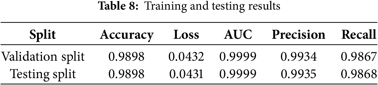
Training was performed using Kaggle’s cloud-based Jupyter notebooks. The computational resources allocated for the experiments included an NVIDIA Tesla T4 GPU, an Intel(R) Xeon(R) CPU running at 2.20 GHz, and 30 GB of RAM. To evaluate the model’s effectiveness during training, standard classification metrics were monitored over multiple epochs. These included accuracy, loss, precision, recall, and AUC (Area Under the ROC Curve) for both the training and validation sets. These metrics provide a comprehensive view of the model’s learning behavior, convergence, and generalization. The final results of the validation set in Table 8 showed excellent performance, with a validation accuracy of 0.9898, AUC of 0.9999, precision of 0.9934, recall of 0.9867, and validation loss of 0.0432.

Near the end of the loss and accuracy plots in Fig. 4a,b, you can observe a spike-and-recovery pattern. This spike, visible particularly around epoch 92, corresponds to the fine-tuning phase carried out during training. In this phase, the model’s configuration was modified, such as updating class weights, or changing the optimizer behavior, causing a temporary increase in both training and validation loss. This disruption is a typical effect when previously frozen layers are made trainable or when learning dynamics are altered mid-training. However, the model quickly readjusted and continued improving. Toward the final epochs, both the training and validation metrics converge smoothly, showing stable performance with validation accuracy closely tracking training accuracy, evidence of strong generalization and minimal overfitting.

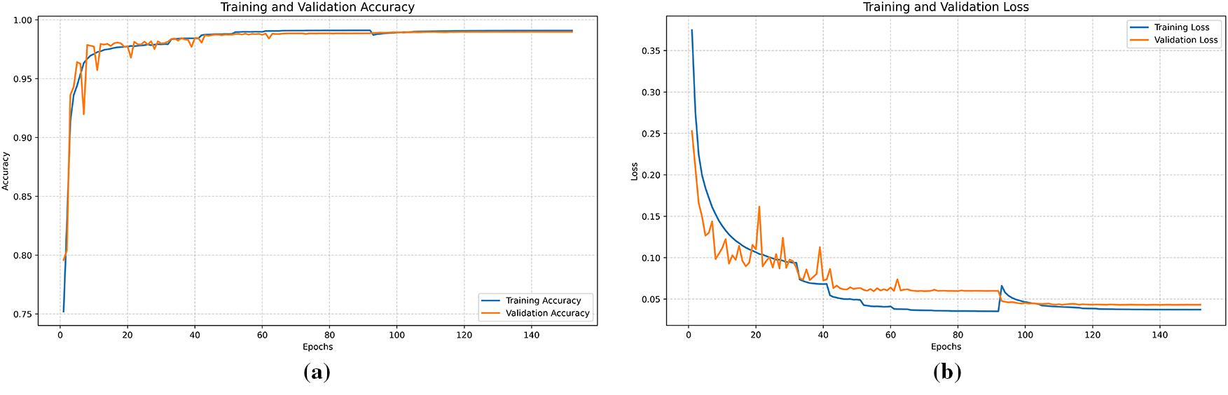
Figure 4: Training and loss curves: (a) Training accuracy vs. validation accuracy (b) Training loss vs. validation loss

7.2 Evaluation on the Testing Set

After training, the model was evaluated on a separate testing split to assess its performance on unseen data. The evaluation metrics reported by the model on the test set were highly consistent with the validation results as shown in Table 8, demonstrating excellent generalization. The test accuracy was 0.9898, AUC was 0.9999, and loss was 0.0431, nearly identical to the final validation metrics. Furthermore, the precision on the test set was 0.9935, while recall was 0.9868, suggesting the model maintained its ability to correctly identify most classes and reduce false positives and false negatives.

7.3 Performance Metrics

The core performance evaluation relied on the metrics of accuracy, precision, recall, and F1-score, each calculated for every class. These metrics are defined as follows; accuracy measures the proportion of total correct predictions, precision evaluates how many of the predicted positives were truly positive, recall measures how many actual positives were identified correctly, f1-score is the harmonic mean of precision and recall.

Accuracy=TP+TNTP+TN+FP+FN(54)

Precision=TPTP+FP(55)

Recall=TPTP+FN(56)

F1=2⋅Precision⋅RecallPrecision+Recall(57)

Additionally, both macro and weighted averages of these metrics were computed to capture class-wise performance. Macro averages compute the unweighted mean across all classes, treating each class equally, while weighted averages account for class imbalance by weighting the metric of each class by its support.

7.4 Reliability Metrics

To further strengthen the reliability and robustness assessment of the model, two widely accepted agreement-based metrics were employed: Cohen’s Kappa Score and Matthews Correlation Coefficient (MCC). Cohen’s Kappa quantifies the agreement between predicted and actual labels while accounting for the agreement occurring by chance [46]. Its formula can be written as Eq. (40)

κ=po−pe1−pe(58)

where po is the observed agreement (i.e., accuracy), and pe is the expected agreement by chance. A value of 1.0 indicates perfect agreement, while a value close to 0 suggests no agreement beyond chance. For this model, Cohen’s Kappa was 0.9848, signifying excellent reliability in classification performance.

Matthews Correlation Coefficient (MCC) is another balanced metric that evaluates the quality of binary and multiclass classifications. It takes into account true and false positives and negatives and is especially informative for imbalanced datasets [47]. It can be calculated using Eq. (41)

MCC=TP⋅TN−FP⋅FN(TP+FP)(TP+FN)(TN+FP)(TN+FN)(59)

For multiclass problems, MCC can be generalized to a more complex form using confusion matrices. In this study, the MCC was computed to be 0.9848, once again affirming the model’s strong consistency across all classes. The full results of Kappa and MCC can be seen in Table 9.

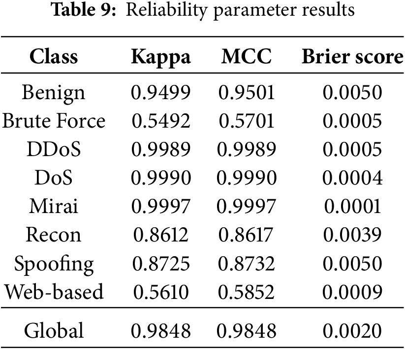
In addition to agreement-based metrics, we further analyzed the reliability of the model using calibration-focused measures: the Brier Score and the Expected Calibration Error (ECE). The Brier Score evaluates the accuracy of probabilistic predictions by measuring the mean squared difference between predicted probabilities and the true outcomes [48]. It can be expressed as Eq. (45):

Brier Score=1N∑i=1N(fi−oi)2(60)

where N is the number of samples, fi is the predicted probability of the positive class, and oi∈{0,1} is the ground-truth outcome. A smaller Brier Score indicates better calibrated and more reliable probability estimates. In this study, the macro-averaged Brier Score was computed as 0.0020, as in Table 9, suggesting that the predicted probabilities are highly consistent with the actual outcomes.

The Expected Calibration Error (ECE) provides a complementary measure by directly quantifying the discrepancy between predicted confidence and empirical accuracy [49]. It is defined as Eq. (46):

ECE=∑m=1M|Bm|n |acc(Bm)−conf(Bm)|(61)

where the predictions are partitioned into M bins, |Bm| is the number of samples in bin m, acc(Bm) is the empirical accuracy, and conf(Bm) is the average predicted confidence in that bin. A lower ECE implies that the model’s confidence is well aligned with its actual accuracy. For the proposed model, the ECE was observed to be 0.0143, which indicates strong probabilistic calibration and reliability of predictions.

To complement these quantitative metrics, calibration curves (reliability diagrams) were also plotted for each class, as shown in Fig. 5. These curves compare the predicted confidence scores against the observed empirical accuracy, where a perfectly calibrated model would follow the diagonal line (y=x). The results indicate that several classes such as DDoS, Mirai, and Spoofing exhibit strong alignment with the diagonal, confirming good calibration. In contrast, classes with fewer samples, such as Brute Force and Web-based attacks, show larger deviations, reflecting reduced reliability in probability estimates for minority classes.

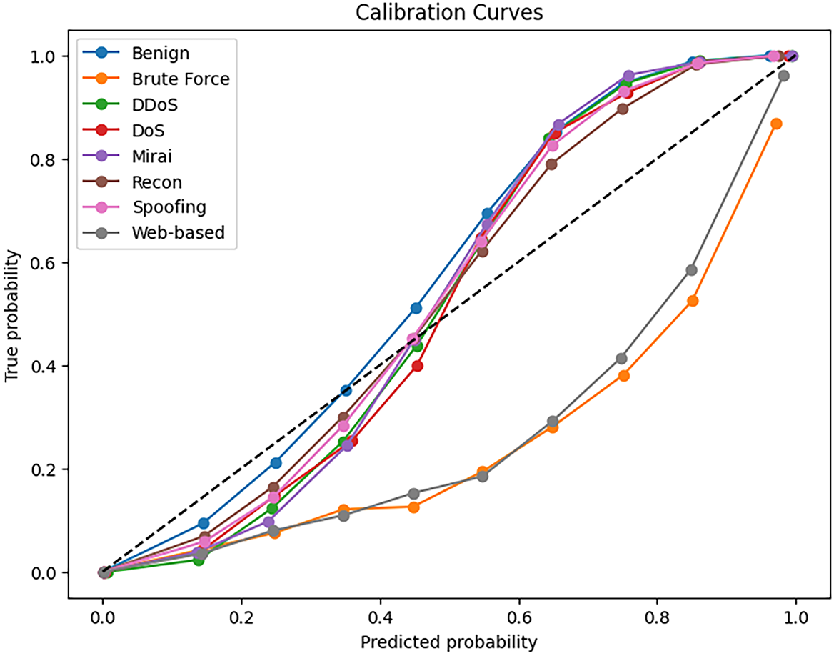
Figure 5: Calibration curves for each class

7.5 Computational Performance

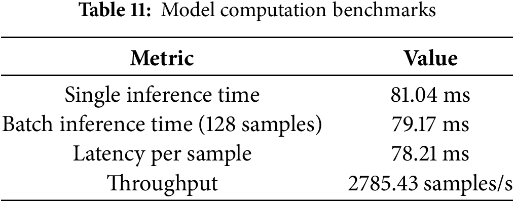
To assess the efficiency of the proposed model, we evaluated its computational performance at both the layer level and the overall inference stage. Table 10 reports the inference times of each individual layer, highlighting that the GRU and dense layers dominate the runtime cost, while earlier convolution and pooling layers incur progressively smaller overheads. This breakdown provides insight into where most of the latency arises and helps identify potential targets for optimization.

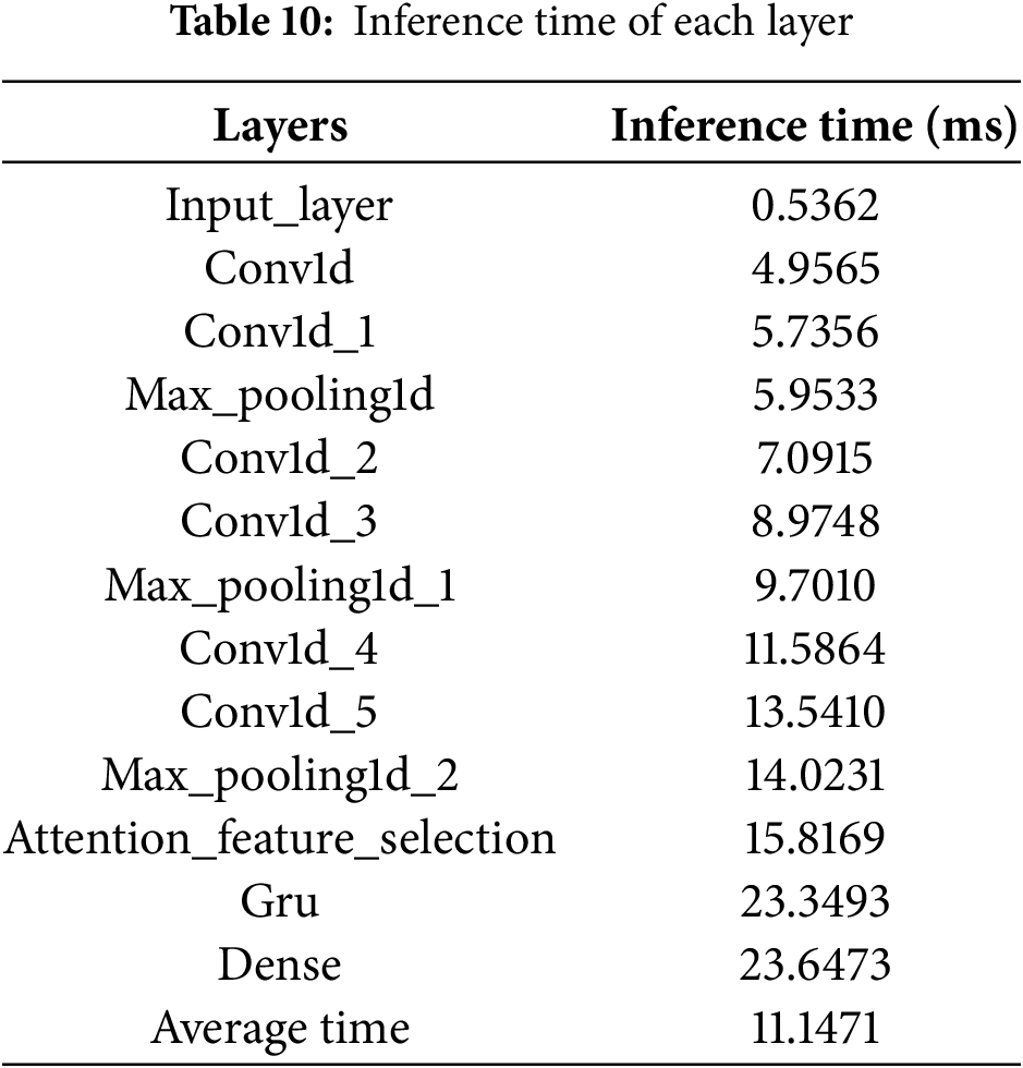
In addition, Table 11 summarizes the overall inference benchmarks. The model achieves a single-sample latency of approximately 81 ms, which is consistent with the cumulative layer timings. Interestingly, when evaluated in batch mode (128 samples), the average per-sample latency drops to about 78 ms due to parallelization. More importantly, given a measured throughput of 2785.43 samples per second, the effective per-sample processing time is theoretically reduced to around 0.36 ms (1/2785.43). This demonstrates that while raw latency per input remains in the tens of milliseconds, high-throughput execution allows the model to scale efficiently in practice.

7.6 Classification Report and Interpretation

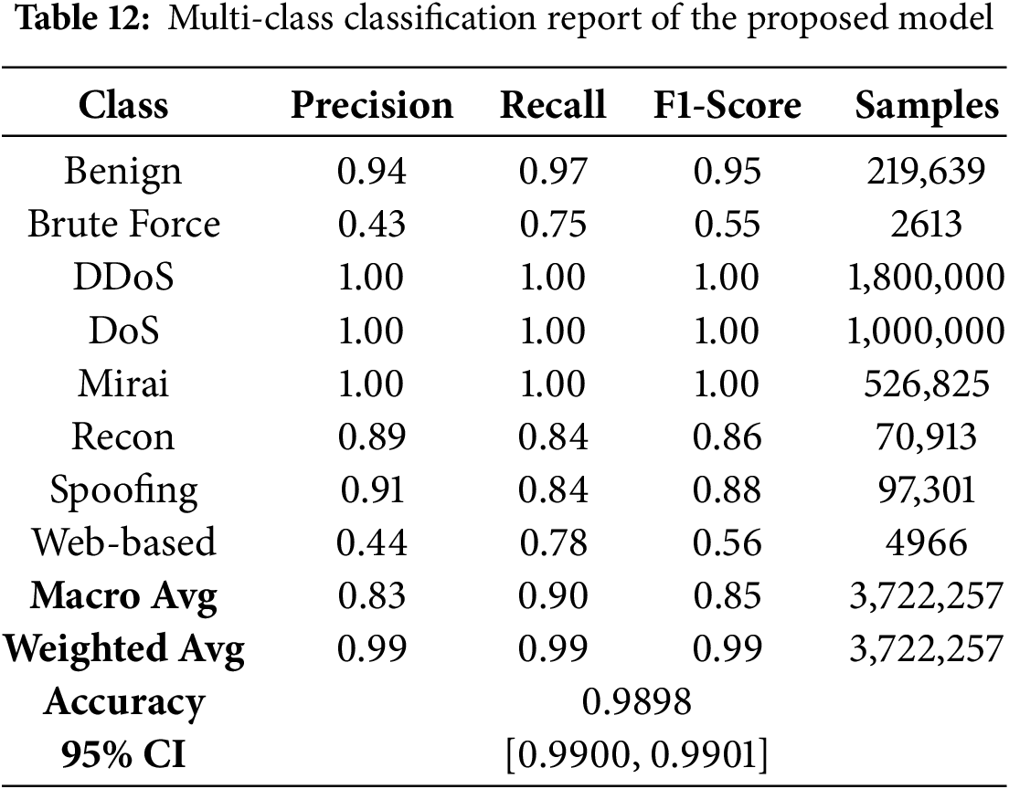
The detailed classification report offers a granular view of how well the model performs on each class in terms of precision, recall, and F1-score, along with the support (number of samples) for each class. Notably, the model achieved perfect or near-perfect scores for high-volume classes such as DDoS, DoS, and Mirai, with F1-scores of 1.00, as evident in Fig. 6. For minority classes like Brute Force and Web-based, which are often more difficult to identify due to their extremely small sample size and similar patterns to benign traffic, the model showed some struggle. Brute Force attacks were detected with a precision of 0.43 and recall of 0.75, leading to an F1-score of 0.55. Similarly, Web-based attacks had a precision of 0.44 and recall of 0.78, with an F1-score of 0.56.

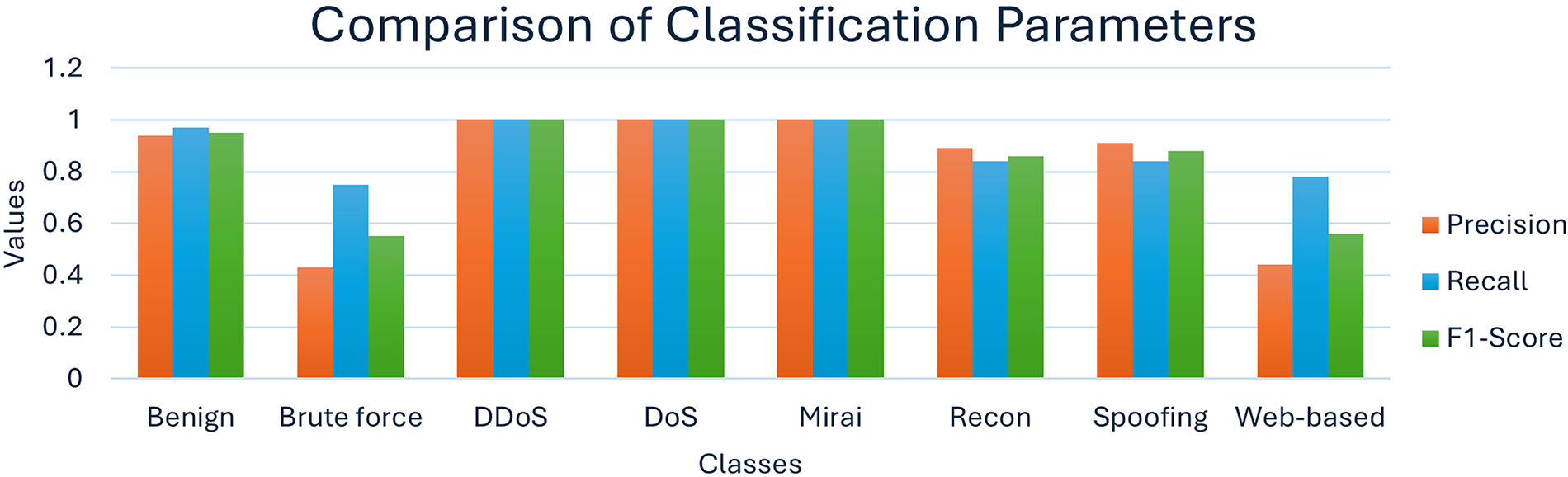
Figure 6: Class-wise comparison of aggregate classification parameters

As shown in Table 12, the macro average F1-score was 0.85, while the weighted average F1-score stood at 0.99, indicating that even though the model struggled with minority classes, its overall performance across the entire dataset was highly satisfactory. The 95% confidence interval further supports its reliability. This classification report underlines the model’s potential to generalize across a diverse and imbalanced intrusion detection dataset with remarkable effectiveness.

In addition, the per-class AUC-PR scores, summarized in Table 13, provide deeper insights into threshold-independent performance. While the biggest attack categories such as DDoS, DoS, and Mirai achieved perfect AUC-PR values of 1.0, Brute Force and Web-based attacks showed weaker performance, reflecting the class imbalance challenges highlighted earlier. The corresponding Precision–Recall curves in Fig. 7 visualize these differences: classes with high AUC-PR exhibit stable precision across a wide recall range, whereas lower-scoring classes show sharper declines in precision as recall increases.

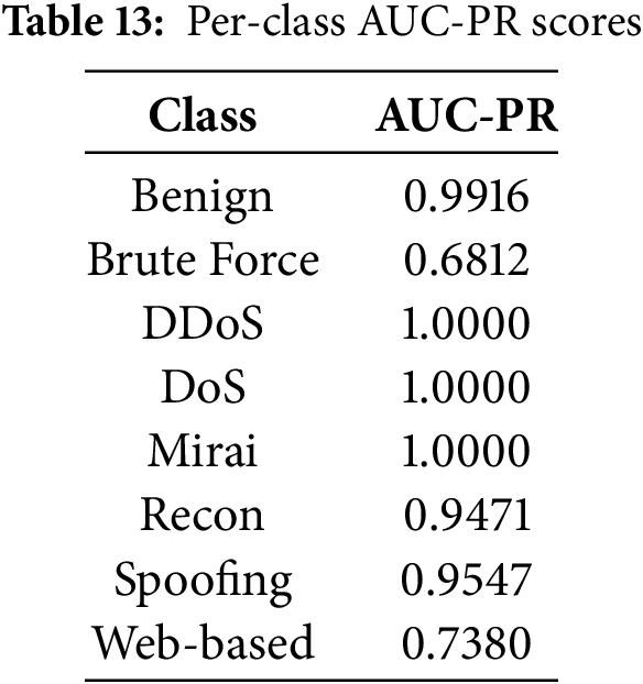
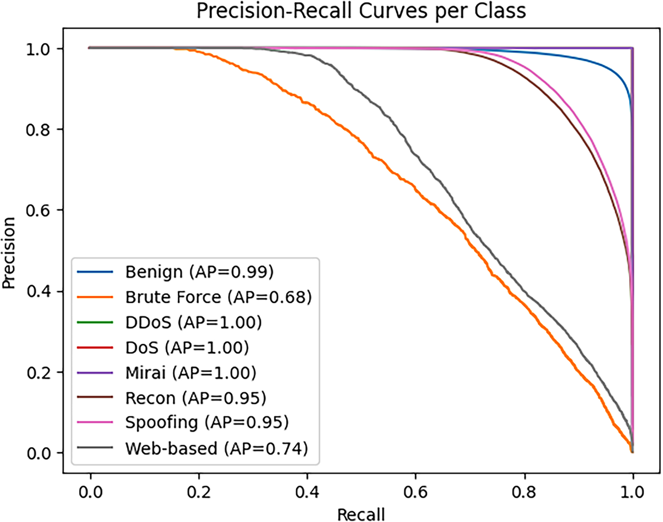
Figure 7: Precision–recall curves per class

From the confusion matrix (Fig. 8), it is clear that the model achieved near-perfect classification performance for the major classes such as DDoS, DoS, and Mirai, with very few misclassifications. These are the largest classes in the dataset, and their clear traffic patterns likely made them easier for the model to learn and distinguish. However, for smaller classes such as Web-based, Brute Force and Recon, the matrix shows occasional confusion, particularly with each other or with benign traffic. These misclassifications are expected given the limited number of training examples for these classes and their sometimes overlapping feature distributions. For example, recon and spoofing attacks are elusive by design. Recon doesn’t flood the network; it probes lightly (e.g., slow scans, banner grabs), which makes it hard to flag without tight thresholds. This resembles like a user browsing or pinging and is often indistinguishable from diagnostics or monitoring tools. Furthermore, it gathers information instead of causing disruptions and IDS systems tuned for anomalies or signatures may find nothing wrong. Similarly, spoofing attacks use false IP/MAC to impersonate trusted sources, due to which tools relying on headers or basic metadata get tricked. Another thing is that spoofing doesn’t generate easily isolatable statistical features, making it hard for AI models without deep context. Web-based attacks are tricky because they exploit legitimate application layers where traffic looks normal, and that breaks many IDS assumptions. Attacks are spread across sessions, domains, URLs, hard to cluster or track unless context is preserved. Web-based intrusion traces are rare and less standardized than brute-force or flood data, and they can fake metadata, making it unreliable. Still, the false positives and false negatives are relatively low, suggesting that even for minority classes, the model maintains a level of precision and recall. The matrix supports the conclusion that the architecture, aided by class balancing and feature selection, was able to generalize well across highly imbalanced class distributions.

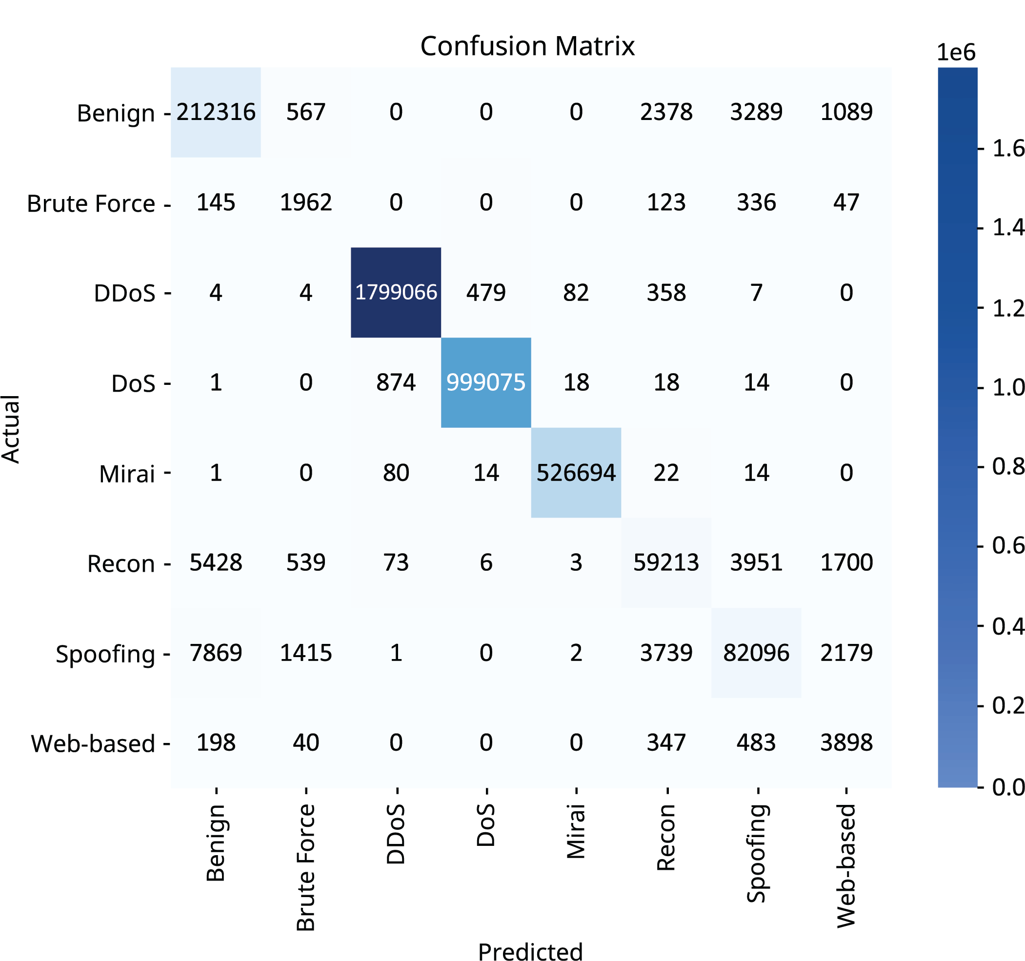
Figure 8: Confusion matrix of the testing split

The normalized confusion matrix (Fig. 9) transforms raw counts into percentages, allowing for a clearer comparison of performance across classes with vastly different sample sizes. Each row sums to 100%, indicating how each actual class was distributed across predicted classes. In this matrix, the diagonal dominance, where the highest values are located along the diagonal confirms that the model is highly accurate in predicting the correct class. For instance, over 99% of DDoS and DoS samples are classified correctly, which is remarkable given their large volume. Smaller classes such as Web-based and Brute Force exhibit weaker diagonal values, typically above 70% but with more off-diagonal leakage, mostly toward classes like Benign or Spoofing. This suggests that while the model is highly confident, there’s still subtle overlap in feature behavior for edge cases or stealthier attacks.

Figure 9: Normalized confusion matrix of the testing split

7.7 SHAP Feature Analysis

Understanding SHAP summary plots is essential for interpreting how each feature influences a model’s prediction decisions. These plots not only show which features are most important but also how they affect the prediction outcomes. Each point in a SHAP summary plot represents a single instance (i.e., a data sample) and its corresponding SHAP value for a specific feature. The horizontal axis shows the SHAP value, this indicates the impact of the feature on the prediction. If the SHAP value is positive, it means the feature pushed the prediction towards a higher probability for the target class (i.e., more likely to be an attack); if it is negative, it pulled the prediction toward a lower probability (i.e., more likely benign).

The color of each point conveys the actual value of the feature for that sample; red points represent high feature values, blue points represent low feature values. So, for example, if you see that high values of the feature IAT (Inter-Arrival Time), depicted by red points, are mostly associated with negative SHAP values, it means longer inter-arrival times reduce the likelihood of an attack prediction, which may imply benign behavior. Conversely, if red points for rst_count cluster around high positive SHAP values, it means that a high number of TCP resets increases the model’s confidence that a sample is an attack. This dual-axis interpretation, SHAP value on the x-axis and feature value in color, gives deep insight into not just importance, but direction and behavior. It helps to answer questions like “Is a high value of this feature a red flag or a sign of normal behavior?”

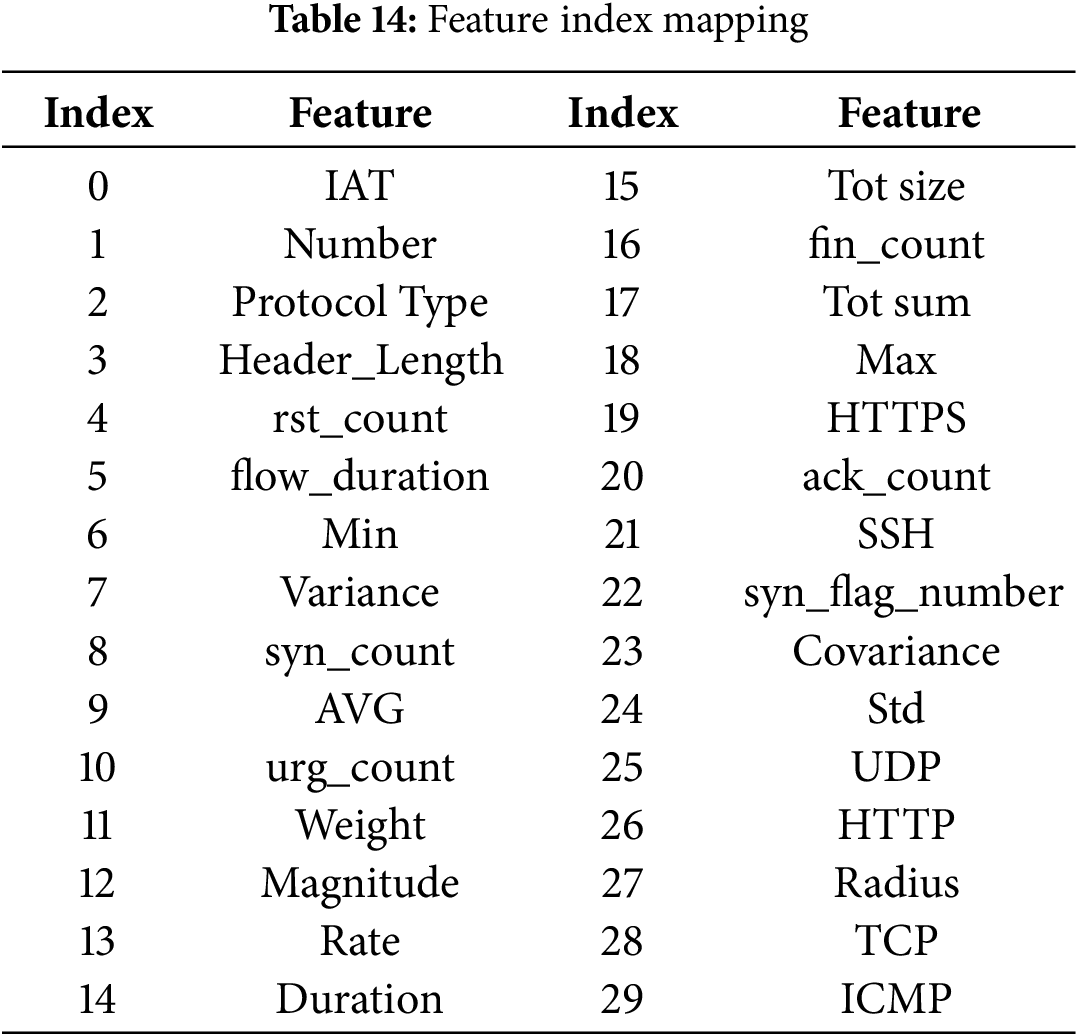
To generate the SHAP explanations for our trained model, 50 randomly selected test samples were used as the explanation set, while 500 background samples were chosen to represent the baseline distribution. Since the model architecture included a custom-built attention layer and was trained using a custom focal loss function, traditional SHAP explainers such as DeepExplainer or GradientExplainer were not suitable due to compatibility limitations with non-standard components. Instead, the more flexible and model-agnostic KernelExplainer was employed. Additionally, a wrapper function was created to adapt the input format to match the model’s expected 3D input shape, ensuring consistency with the time-step-based data structure. This allowed for accurate SHAP value computation even with the non-standard architecture and training configuration. The feature analysis started with the per-class SHAP summary plots which can be seen in Figs. 10 and 11, showing how each feature influenced predictions for each class one by one. The feature index map has also been provided in Table 14.

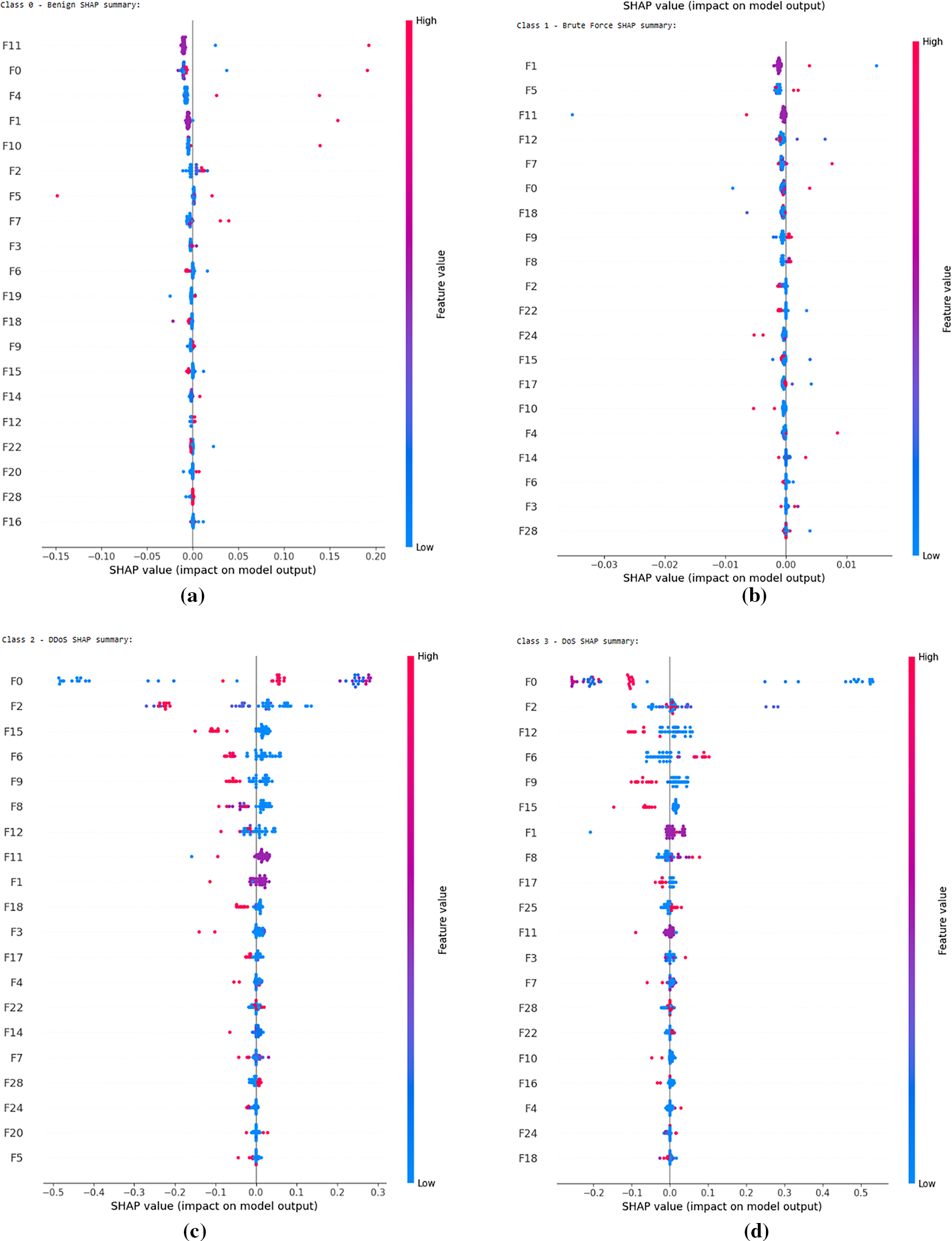
Figure 10: Feature impact for each class using SHAP values (a) Benign (b) Brute Force (c) DDoS (d) DoS

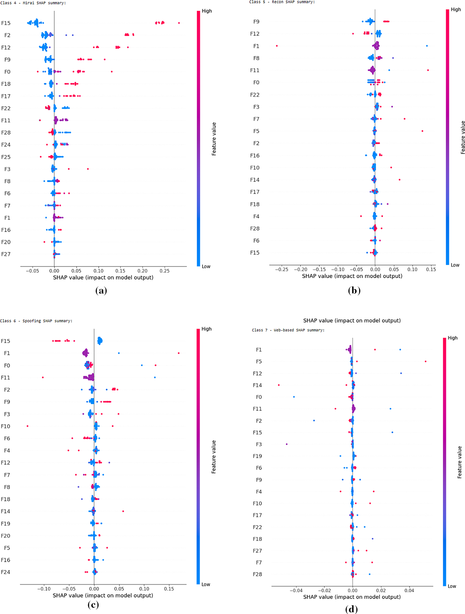
Figure 11: Feature impact for each class using SHAP values (a) Mirai (b) Recon (c) Spoofing (d) Web-based

There appear to be some patterns between the most impactful features of different classes. F0 (IAT) and F1 (Number) seem to be the most defining features among most classes while F2 (Protocol Type) and F6 (Min), F9 (AVG), F12 (Magnitude) and F15 (Tot size) also have a great impact among the three easiest classes to predict. The minor classes such as spoofing and recon also seem to have more ambiguity in signifying the impact of different features. Reasons for these patterns will be further discussed in the next sub-section.

Next is the mean SHAP (directional) summary plot in Fig. 12, which illustrates the average signed contribution of each feature to the model’s predictions. Each horizontal point represents the average SHAP value for a feature across all samples, where positive values indicate a feature pushed predictions toward the positive class (likely an attack), and negative values suggest it contributed to predicting the negative class. This type of SHAP plot helps reveal directionality, i.e., how features influence the model, not just how much.

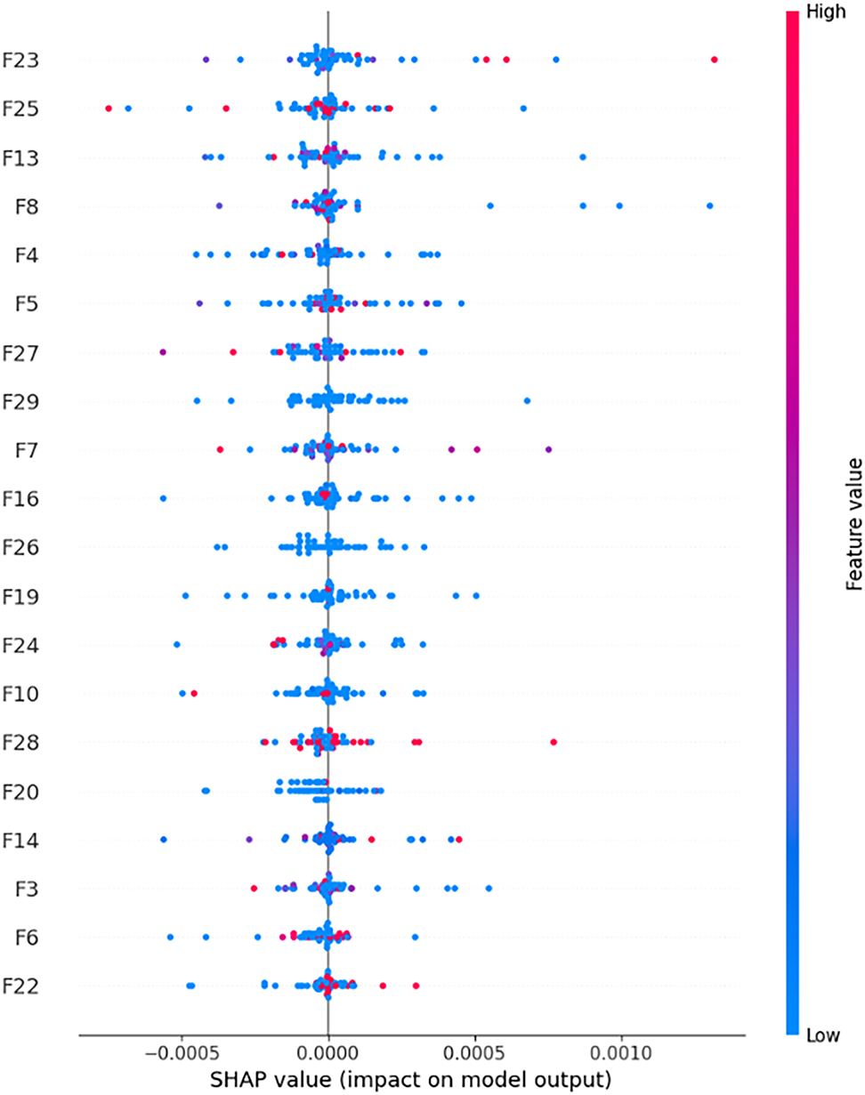
Figure 12: Mean (directional) SHAP plot

From the plot, we see that features like F16 (fin_count), F8 (syn_count), F23 (Covariance) and F7 (Variance) lean slightly to the right of the center line, suggesting they generally increase the model’s confidence in identifying an attack. These features, related to the magnitude of traffic, are consistent with malicious behavior, high frequency of connection flags (like FIN or Variance) often correlates with scans, brute-force attempts, or denial-of-service activities. On the other hand, features such as F19 (HTTPS), F20 (ack_count), F26 (HTTP) and F27 (Radius) lean more to the left, meaning they typically contribute negatively toward attack classification, suggesting that their presence is more indicative of benign traffic patterns in this dataset. For example, HTTPS is a standard protocol for secure communication. Attack traffic often avoids HTTPS due to encryption overhead or uses malformed HTTPS headers.

This plot is especially valuable because it captures not just importance but interpretability with polarity. It answers questions like “Is a feature positively or negatively correlated with attack behavior?” In contrast to absolute SHAP plots that only give magnitude, this directional SHAP view reveals how the model is using each feature. For example, a feature with a high absolute SHAP value but a neutral mean directional SHAP might be used equally in both directions, which could make it important, but less interpretable. Moreover, seeing many features clustered around the center, such as F27 (Radius), F26 (HTTP), and F25 (UDP), implies that these features may have little to no consistent directional influence, and might only be useful in very specific attack types or are highly dependent on context. These observations can inform decisions about feature pruning, simplification, or targeted model improvements.

7.8 Selecting Top-k Features

Finally, the Mean Absolute SHAP values provide a robust and unbiased way to evaluate how much each feature contributes to the model’s predictions, regardless of whether the contribution pushes the prediction higher or lower. Unlike directional SHAP values, which tell us the sign of the impact (positive or negative), the magnitude-only SHAP values capture the overall influence of a feature across all predictions and classes, making them especially useful for tasks like feature selection and ranking. In the context of our intrusion detection task, where model interpretability and efficiency are crucial, mean absolute SHAP values offer the clearest insight into which features consistently carry the most predictive power. These values average the absolute SHAP contributions of each feature across all samples and classes, giving a single score that represents overall importance. This approach is particularly valuable when working with multi-class tabular data, where directionality might vary across classes but importance remains high. All 30 selected features were first plotted out based on the evaluation of their overall contribution to the model’s predictions using mean absolute SHAP values, as illustrated in Fig. 13.

Figure 13: Bar graph showing the feature importance of all 30 features

Subsequently, the top-k most influential features were visualized using a SHAP summary bar plot (Fig. 14). In this study, k was set to 20 for post-training explanation of important features, though this value is flexible; depending on time or resource constraints, a smaller subset such as the top 15 or even top 10 features can also be reused effectively. Features can even be selected based on the per class impact depending on the use-case.

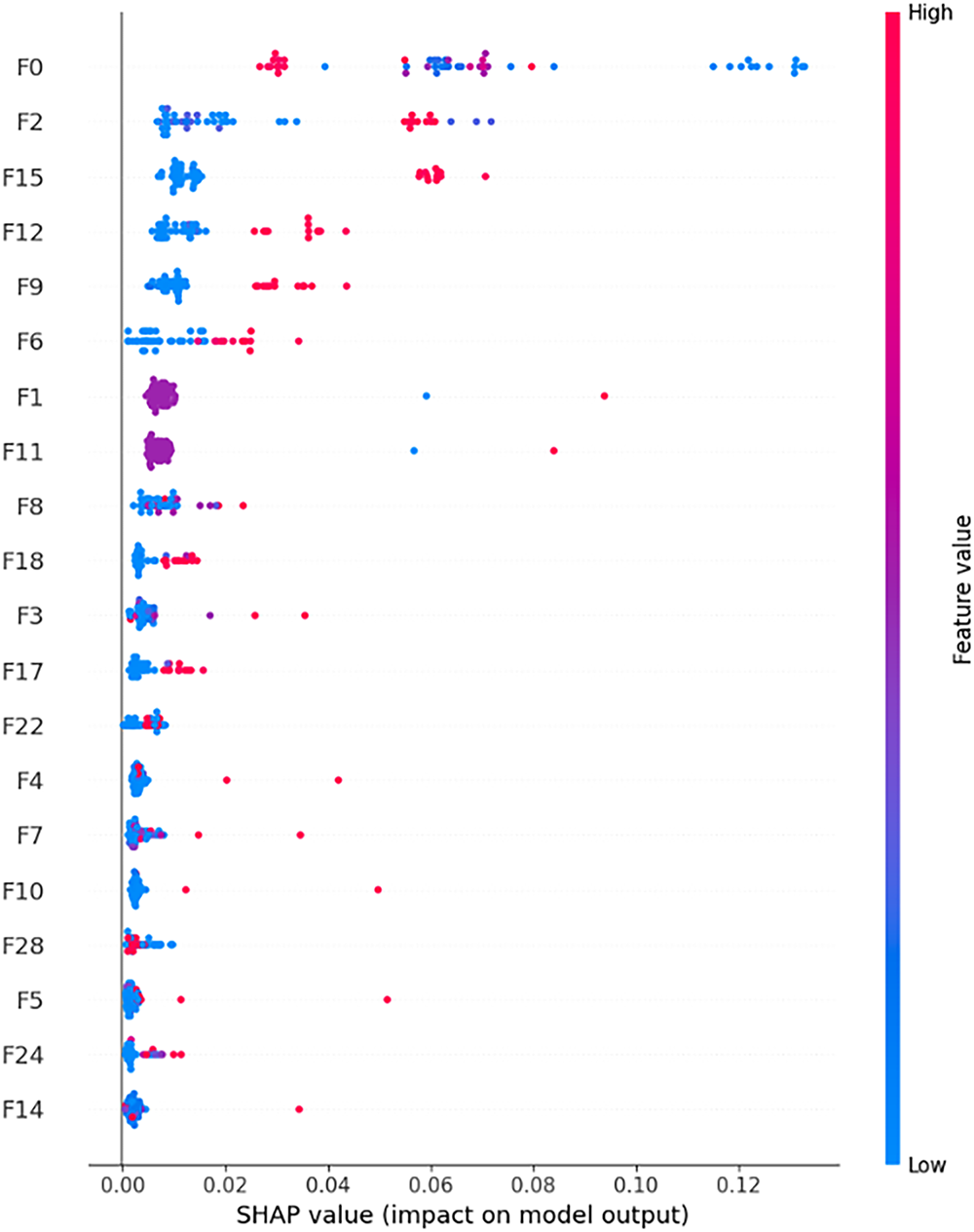
Figure 14: Absolute mean (magnitude only) SHAP plot

Finally, a bar chart (Fig. 15) used for displaying these top features, this time labeled with their actual names, is presented to support interpretation. The visualization is followed by a detailed rationalization of why each feature plays a significant role in the model’s decision-making process.

Figure 15: Top 20 selected feature index mapping along with their importance

Rationalization of Important Features

The mean absolute SHAP values reveal a highly uneven contribution of features, with only four surpassing the 0.01 threshold. Inter-Arrival Time (IAT) dominates with a SHAP value of 0.0724, reflecting its critical role in distinguishing benign from malicious traffic, as timing irregularities are strong indicators of anomalies such as DDoS or scanning. Protocol type also ranks high, since specific attacks often exploit TCP, UDP, or ICMP. Features such as Total (flow size), Magnitude, and Average capture volumetric and behavioral differences between normal and automated traffic, while Min and Max values highlight extreme cases typical of SYN floods or resource exhaustion attempts. Packet- and flag-based indicators (e.g., syn_count, syn_flag_number, rst_count, urg_flag) further support detection of flooding and brute-force activity. Statistical descriptors like Variance, Standard Deviation, and Flow Duration provide insight into flow consistency and persistence, differentiating steady human activity from repetitive bot traffic. Together, SHAP highlights that AutoSHARC relies on a compact but semantically meaningful set of timing, protocol, statistical, and flag-based features for robust intrusion detection.

This absolute SHAP ranking is instrumental in creating a reusable and optimized feature subset, which not only reduces model complexity and training time but also enhances generalization performance. It helps eliminate redundant or noisy features, ensures better resource efficiency, and makes the model more interpretable, a critical factor in security-related applications where explainability is just as important as accuracy.

8  Comparative Analysis of the Proposed Model

The purpose of this comparative analysis is to contextualize the performance of the proposed CNN-Attention-GRU model against a wide range of models previously applied to the CIC IoT 2023 dataset. As seen in Table 15, the models span across various deep learning and machine learning architectures, including LSTM, CNNs, RNNs, transformers, random forests, and boosting-based classifiers. Many of these studies did not incorporate any formal feature selection techniques, relying solely on the raw or preprocessed input features. In contrast, a few leveraged specific selection strategies such as Recursive Feature Elimination or correlation-based methods to improve learning efficiency. Our approach stands out not only for its architectural design tailored for intelligent feature selection but also for integrating an ensemble of feature selectors, Boruta, LightGBM, and SHAP, to optimize the input space before training. Despite not using the transformer-based or ensemble learning models with the highest reported accuracy, our model achieves a competitive accuracy of 98.98%, validating the effectiveness of using targeted feature selection to strike a balance between performance, and interpretability. In addition, as shown in Table 16, the proposed CNN-Attention-GRU model demonstrates superior resource efficiency, achieving significantly smaller model size and faster edge inference time compared to existing lightweight IDS models.

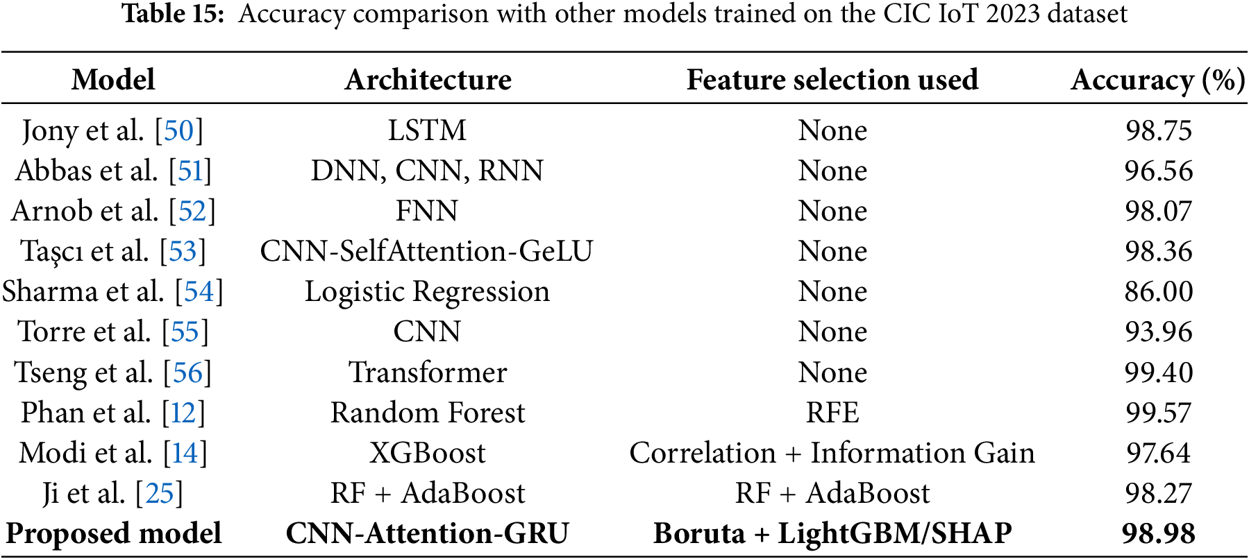
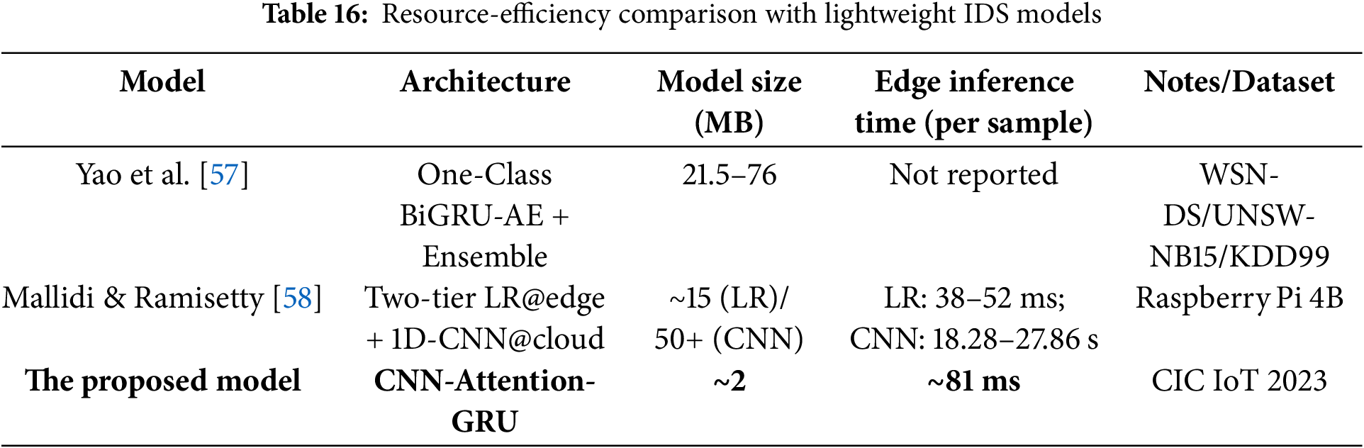
It is important to emphasize that the accuracy figures reported in most, if not all, existing papers on the CIC IoT 2023 dataset often reflect weighted accuracy, which, while useful in some cases, does not present a complete or fair picture of a model’s true performance across all classes. Weighted metrics, as those mentioned in Table 12 are heavily influenced by class distribution, and in highly imbalanced datasets like CIC IoT 2023, they can give an illusion of superior performance even if minority classes are poorly predicted. In contrast, macro metrics, including macro accuracy, precision, recall, and F1-score, treat each class equally regardless of size, and therefore provide a much clearer assessment of per-class effectiveness.

In this work, only around 40% of the total dataset was used during training, which slightly helped reduce class imbalance. However, many papers neither balance their datasets nor report macro scores or confusion matrices in case of an imbalance. For instance, Tseng et al. [56], who report an impressive 99.40% accuracy using a transformer-based model, only include weighted scores in their evaluation. When the macro scores are extracted from their published confusion matrix, a different story emerges: the macro precision drops to 0.9189, the recall falls to 0.7447, and the macro F1-score plummets to just 0.7818. These figures reveal significant underperformance on minority attack classes. What further undermines the validity of such high reported accuracies is that the full dataset used in such studies contained over 95 million samples from just the major classes. In such a skewed scenario, achieving high accuracy or weighted metrics becomes trivial, often limited more by RAM capacity than algorithmic strength. This highlights the urgent need for papers to include macro-based metrics and confusion matrices as standard practice to ensure fairness, reproducibility, and a true reflection of a model’s utility in detecting rare but critical threats.

Ablation Study

To further validate the effectiveness of the proposed framework, an ablation study was conducted by comparing the performance of different feature selection strategies and architectural variations. As shown in Table 17, XGBoost, one of the strongest machine learning algorithms and a simple MLP with two dense layers were chosen as baseline models and trained with the same features selected as for our model. They demonstrated strong accuracies (98.90% and 98.63%, respectively), but their macro F1-scores lagged behind the proposed model. Similarly, removing the attention and GRU mechanisms from the CNNs reduced the balance across classes, as evidenced by the drop in macro F1. In contrast, the proposed model achieved the best overall performance with a validation accuracy of 98.98% and a macro F1-score of 84.78, underscoring the importance of both the hybrid feature selection approach and the architectural enhancements in improving generalization and robustness across imbalanced classes.

9  Conclusion

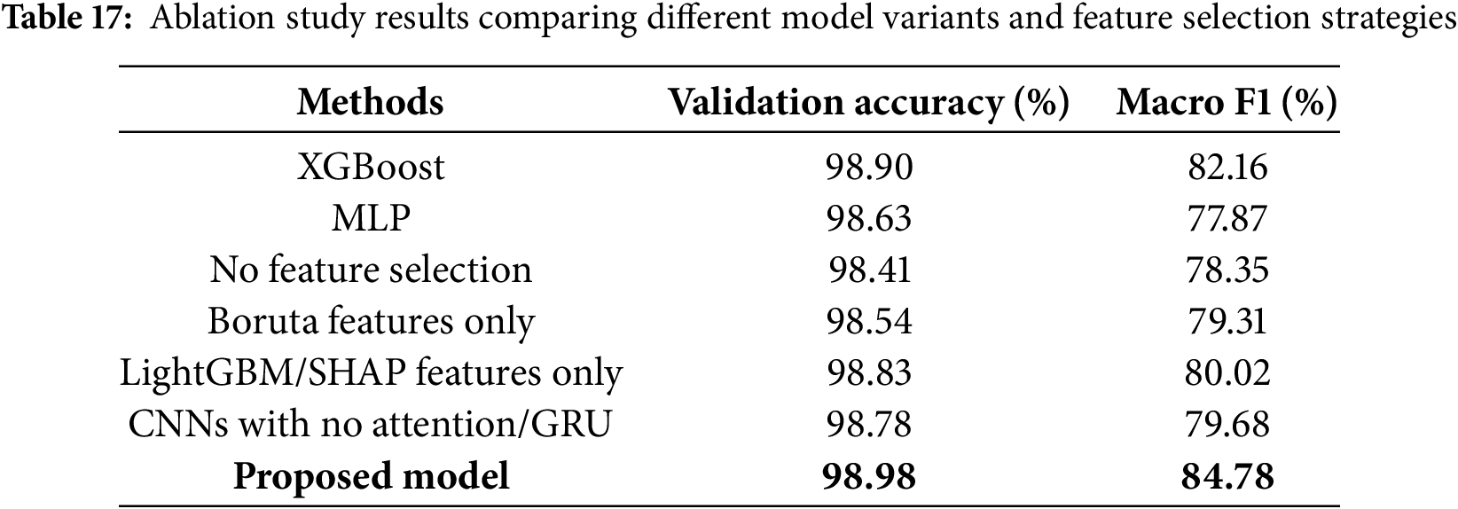
This paper presented AutoSHARC, a feedback-driven explainable feature selection framework designed for intrusion detection in IoT and programmable networks. By addressing the dual challenges of high-dimensional network traffic and the need for real-time interpretability, AutoSHARC enhanced detection accuracy while contributing to the preservation of Quality of Service (QoS). By combining Boruta and LightGBM/SHAP for robust feature preselection, and employing post-hoc SHAP refinement for iterative retraining, AutoSHARC reduced input dimensionality while preserving interpretability and detection performance. This feedback loop enabled the model to self-optimize by focusing only on the most impactful features, improving scalability and reducing computational cost. Extensive evaluations on the CIC IoT 2023 dataset showed that AutoSHARC achieved a testing accuracy of 98.98%, an F1-score of 99.02%, recall of 98.68%, and precision of 99.35%. Robustness was further confirmed with a Matthews Correlation Coefficient (MCC) of 0.9848 as well as a Cohen’s Kappa of 0.9848. In addition, the final model maintained a compact footprint of approximately 2 MB with 531,272 trainable parameters, making it resource-efficient and suitable for real-time QoS-sensitive environments. Despite these strong results, AutoSHARC shares common limitations with many supervised learning approaches. Its performance is tightly linked to the training distribution, meaning that unseen or rapidly evolving attack types may reduce effectiveness until retraining is performed. Similarly, while the framework is model-agnostic in feature selection, its current design is tailored to tabular intrusion detection data and may require adaptation for domains with strong temporal or spatial dependencies. Future work will extend AutoSHARC for integration with SDN controllers and 5G network slicing platforms, enabling real-time deployment at the network edge. Such integration would allow programmable networks to dynamically adapt to evolving threats while preserving QoS across diverse services and applications, thereby advancing the broader vision of AI- and ML-driven intelligent network management.

Acknowledgement: This research was supported by Princess Nourah bint Abdulrahman University Researchers Supporting Project number (PNURSP2025R333), Princess Nourah bint Abdulrahman University, Riyadh, Saudi Arabia.

Funding Statement: Princess Nourah bint Abdulrahman University Researchers Supporting Project number (PNURSP2025R333), Princess Nourah bint Abdulrahman University, Riyadh, Saudi Arabia.

Author Contributions: The authors confirm contribution to the paper as follows: Conceptualization, Muhammad Shahbaz Khan and Muhammad Saad Farooqui; methodology, Muhammad Saad Farooqui and Muhammad Shahbaz Khan; software, Muhammad Saad Farooqui and Aizaz Ahmad Khattak; validation, Bakri Hossain Awaji and Nazik Alturki; investigation, Nazik Alturki and Noha Alnazzawi; data curation, Noha Alnazzawi and Muhammad Hanif; writing—original draft preparation, Muhammad Saad Farooqui and Muhammad Shahbaz Khan; writing—review and editing, Aizaz Ahmad Khattak and Muhammad Hanif; supervision, Muhammad Shahbaz Khan. All authors reviewed the results and approved the final version of the manuscript.

Availability of Data and Materials: The data that support the findings of this study are openly available in University of New Brunswick Repository at https://www.unb.ca/cic/datasets/iotdataset-2023.html, accessed on 10 May 2025.

Ethics Approval: Not applicable.

Conflicts of Interest: The authors declare no conflicts of interest to report regarding the present study.

References

1. Alnaim AK. Securing 5G virtual networks: a critical analysis of SDN, NFV, and network slicing security. Int J Inf Secur. 2024;23(6):3569–89. doi:10.1007/s10207-024-00900-5. [Google Scholar] [CrossRef]

2. Le A, Loo J, Lasebae A, Aiash M, Luo Y. 6LoWPAN: a study on QoS security threats and countermeasures using intrusion detection system approach. Int J Communicat Syst. 2012;25(9):1189–212. doi:10.1002/dac.2356. [Google Scholar] [CrossRef]

3. Venkatesh B, Anuradha J. A review of feature selection and its methods. Cybern Inf Technol. 2019;19(1):3–26. doi:10.2478/cait-2019-0001. [Google Scholar] [CrossRef]

4. Guyon I, Elisseeff A. An introduction to variable and feature selection. J Mach Learn Res. 2003;3(7–8):1157–82. [Google Scholar]

5. Torabi M, Udzir NI, Abdullah MT, Yaakob R. A review on feature selection and ensemble techniques for intrusion detection system. Int J Adv Comput Sci Appl. 2021;12(5):538–53. doi:10.14569/ijacsa.2021.0120566. [Google Scholar] [CrossRef]

6. Nimbalkar P, Kshirsagar D. Feature selection for intrusion detection system in Internet-of-Things (IoT). ICT Express. 2021;7(2):177–81. doi:10.1016/j.icte.2021.04.012. [Google Scholar] [CrossRef]

7. Yin Y, Jang-Jaccard J, Xu W, Singh A, Zhu J, Sabrina F, et al. IGRF-RFE: a hybrid feature selection method for MLP-based network intrusion detection on UNSW-NB15 dataset. J Big Data. 2023;10(1):1–26. doi:10.1186/s40537-023-00694-8. [Google Scholar] [CrossRef]

8. Tsimenidis S, Lagkas T, Rantos K. Deep learning in IoT intrusion detection. J Netw Syst Manag. 2022;30(1):8. doi:10.1007/s10922-021-09621-9. [Google Scholar] [CrossRef]

9. Chen X, Liu M, Wang Z, Wang Y. Explainable deep learning-based feature selection and intrusion detection method on the internet of things. Sensors. 2024;24(16):5223. doi:10.3390/s24165223. [Google Scholar] [PubMed] [CrossRef]

10. Iftikhar N, Rehman MU, Shah MA, Alenazi MJF, Ali J. Intrusion detection in NSL-KDD dataset using hybrid self-organizing map model. Comput Model Eng Sci. 2025;143(1):639–71. doi:10.32604/cmes.2025.062788. [Google Scholar] [CrossRef]

11. Wardana AA, Sukarno P, Basuki S, Utomo SB. Federated random forest with feature selection for collaborative intrusion detection in internet of things. Procedia Comput Sci. 2024;246:20–9. doi:10.1016/j.procs.2024.09.193. [Google Scholar] [CrossRef]

12. Phan VA, Jerabek J, Malina L. Comparison of multiple feature selection techniques for machine learning-based detection of IoT attacks. In: Proceedings of the 19th International Conference on Availability, Reliability and Security; 2024 Jul 30–Aug 2; Vienna, Austria. p. 1–10. [Google Scholar]

13. Chikkalwar SR, Garapati Y. An effective intrusion detection system based on feature selection and regularized long short-term memory classifier. Multimed Tools Appl. 2025;84(35):43959–82. doi:10.1007/s11042-025-20889-w. [Google Scholar] [CrossRef]

14. Modi P. Towards efficient machine learning method for IoT DDoS attack detection. arXiv:2408.10267. 2024. [Google Scholar]

15. Wang Z, Li Z, He D, Chan S. A lightweight approach for network intrusion detection in industrial cyber-physical systems based on knowledge distillation and deep metric learning. Expert Syst Appl. 2022;206(4):117671. doi:10.1016/j.eswa.2022.117671. [Google Scholar] [CrossRef]

16. Wahab F, Ma S, Liu X, Zhao Y, Shah A, Ali B. A ranked filter-based three-way clustering strategy for intrusion detection in highly secure IoT networks. Comput Elect Eng. 2025;127(3):110514. doi:10.1016/j.compeleceng.2025.110514. [Google Scholar] [CrossRef]

17. Westphal C, Hailes S, Musolesi M. Feature selection for network intrusion detection. In: Proceedings of the 31st ACM SIGKDD Conference on Knowledge Discovery and Data Mining V. 1; 2025 Aug 3–7; Toronto, ON, Canada. p. 1599–610. [Google Scholar]

18. Shoukat S, Gao T, Javeed D, Saeed MS, Adil M. Trust my IDS: an explainable AI integrated deep learning-based transparent threat detection system for industrial networks. Comput Secur. 2025;149(2):104191. doi:10.1016/j.cose.2024.104191. [Google Scholar] [CrossRef]

19. Younisse R, Ahmad A, Abu Al-Haija Q. Explaining intrusion detection-based convolutional neural networks using shapley additive explanations (shap). Big Data Cogn Comput. 2022;6(4):126. doi:10.3390/bdcc6040126. [Google Scholar] [CrossRef]

20. Pande S, Khamparia A. Explainable deep neural network based analysis on intrusion detection systems. Comput Sci. 2023;24(1):97–111. doi:10.7494/csci.2023.24.1.4551. [Google Scholar] [CrossRef]

21. Gaspar D, Silva P, Silva C. Explainable AI for intrusion detection systems: lIME and SHAP applicability on multi-layer perceptron. IEEE Access. 2024;12(11):30164–75. doi:10.1109/access.2024.3368377. [Google Scholar] [CrossRef]

22. Ravi V, Chaganti R, Alazab M. Recurrent deep learning-based feature fusion ensemble meta-classifier approach for intelligent network intrusion detection system. Comput Elect Eng. 2022;102(3):108156. doi:10.1016/j.compeleceng.2022.108156. [Google Scholar] [CrossRef]

23. Wahab F, Ma S, Zhao Y, Shah A. An explainable three-way neural network approach for intrusion detection in IoT ecosystem. Inter Things. 2025;33(1):101722. doi:10.1016/j.iot.2025.101722. [Google Scholar] [CrossRef]

24. Cerasuolo F, Bovenzi G, Ciuonzo D, Pescapè A. Adaptable, incremental, and explainable network intrusion detection systems for internet of things. Eng Appl Artif Intell. 2025;144(2):110143. doi:10.1016/j.engappai.2025.110143. [Google Scholar] [CrossRef]

25. Ji R, Selwal A, Kumar N, Padha D. Cascading bagging and boosting ensemble methods for intrusion detection in cyber-physical systems. Secur Priv. 2025;8(1):e497. doi:10.1002/spy2.497. [Google Scholar] [CrossRef]

26. Chohra A, Shirani P, Karbab EB, Debbabi M. Chameleon: optimized feature selection using particle swarm optimization and ensemble methods for network anomaly detection. Comput Secur. 2022;117:102684. doi:10.1016/j.cose.2022.102684. [Google Scholar] [CrossRef]

27. Zada I, Omran E, Jan S, Alfraihi H, Alsalamah S, Alshahrani A, et al. Enhancing IoT cybersecurity through lean-based hybrid feature selection and ensemble learning: a visual analytics approach to intrusion detection. PLoS One. 2025;20(7):e0328050. doi:10.1371/journal.pone.0328050. [Google Scholar] [PubMed] [CrossRef]

28. Otokwala U, Petrovski A, Kalutarage H. Optimized common features selection and deep-autoencoder (OCFSDA) for lightweight intrusion detection in Internet of things. Int J Inform Secur. 2024;23(4):2559–81. doi:10.1007/s10207-024-00855-7. [Google Scholar] [CrossRef]

29. Ji R, Kumar N, Padha D. Hybrid enhanced intrusion detection frameworks for cyber-physical systems via optimal features selection. Indian J Sci Technol. 2024;17(30):3069–79. doi:10.17485/ijst/v17i30.1794. [Google Scholar] [CrossRef]

30. Bakro M, Kumar RR, Husain M, Ashraf Z, Ali A, Yaqoob SI, et al. Building a cloud-IDS by hybrid bio-inspired feature selection algorithms along with random forest model. IEEE Access. 2024;12:8846–74. doi:10.1109/access.2024.3353055. [Google Scholar] [CrossRef]

31. Dasari AK, Biswas SK, Baruah B, Purkayastha B, Das S. Intrusion detection system using stacked ensemble learning with light gradient boosting machine and decision tree. In: Proceedings of International Conference on Network Security and Blockchain Technology (ICNSBT 2024). Singapore: Springer; 2024. p. 291–303. [Google Scholar]

32. Neto ECP, Dadkhah S, Ferreira R, Zohourian A, Lu R, Ghorbani AA. CICIoT2023: a real-time dataset and benchmark for large-scale attacks in IoT environment. Sensors. 2023;23(13):5941. doi:10.3390/s23135941. [Google Scholar] [PubMed] [CrossRef]

33. Jayasinghe WLP, Deo RC, Ghahramani A, Ghimire S, Raj N. Deep multi-stage reference evapotranspiration forecasting model: multivariate empirical mode decomposition integrated with the boruta-random forest algorithm. IEEE Access. 2021;9:166695–708. doi:10.1109/access.2021.3135362. [Google Scholar] [CrossRef]

34. Hur JH, Ihm SY, Park YH. A variable impacts measurement in random forest for mobile cloud computing. Wirel Commun Mob Comput. 2017;2017(1):6817627. doi:10.1155/2017/6817627. [Google Scholar] [CrossRef]

35. Duan S, Huang S, Bu W, Ge X, Chen H, Liu J, et al. LightGBM low-temperature prediction model based on LassoCV feature selection. Math Probl Eng. 2021;2021(1):1776805. doi:10.1155/2021/1776805. [Google Scholar] [CrossRef]

36. Chen W, Yang H, Yin L, Luo X. Large-scale IoT attack detection scheme based on LightGBM and feature selection using an improved salp swarm algorithm. Sci Rep. 2024;14(1):19165. doi:10.1038/s41598-024-69968-2. [Google Scholar] [PubMed] [CrossRef]

37. Alshehri MS, Ahmad J, Almakdi S, Al Qathrady M, Ghadi YY, Buchanan WJ. Skipgatenet: a lightweight CNN-lstm hybrid model with learnable skip connections for efficient botnet attack detection in IoT. IEEE Access. 2024;12(1):35521–38. doi:10.1109/access.2024.3371992. [Google Scholar] [CrossRef]

38. Suárez-Paniagua V, Segura-Bedmar I. Evaluation of pooling operations in convolutional architectures for drug-drug interaction extraction. BMC Bioinformatics. 2018;19(Suppl 8):209. doi:10.1186/s12859-018-2195-1. [Google Scholar] [PubMed] [CrossRef]

39. Woo S, Park J, Lee JY, Kweon IS. CBAM: convolutional block attention module. In: European Conference on Computer Vision. Cham, Switzerland: Springer; 2018. p. 3–19. [Google Scholar]

40. Hassanin M, Anwar S, Radwan I, Khan FS, Mian A. Visual attention methods in deep learning: an in-depth survey. arXiv:2204.07756. 2022. [Google Scholar]

41. Shiri FM, Perumal T, Mustapha N, Mohamed R. A comprehensive overview and comparative analysis on deep learning models: CNN, RNN, LSTM, GRU. arXiv:2305.17473. 2023. [Google Scholar]

42. Hinton G, Srivastava N, Swersky K. Neural networks for machine learning lecture 6a overview of mini-batch gradient descent. Lecture Notes Distributed in CSC321 of University of Toronto; 2012. [cited 2025 Oct 12]. Available from: https://www.cs.toronto.edu/~hinton/coursera/lecture6/lec6.pdf. [Google Scholar]

43. Zou F, Shen L, Jie Z, Zhang W, Liu W. A sufficient condition for convergences of adam and RMSProp. In: 2019 IEEE/CVF Conference on Computer Vision and Pattern Recognition (CVPR); 2019 Jun 15–20; Long Beach, CA, USA. p. 11119–27. [Google Scholar]

44. Reddi SJ, Kale S, Kumar S. On the convergence of adam and beyond. arXiv:1904.09237. 2019. [Google Scholar]

45. Lin TY, Goyal P, Girshick R, He K, Dollár P. Focal loss for dense object detection. In: Proceedings of the 2017 IEEE International Conference on Computer Vision; 2017 Oct 22–29; Venice, Italy. p. 2980–8. [Google Scholar]

46. Yilmaz AE, Demirhan H. Weighted kappa measures for ordinal multi-class classification performance. Appl Soft Comput. 2023;134(1):110020. doi:10.1016/j.asoc.2023.110020. [Google Scholar] [CrossRef]

47. Catillo M, Pecchia A, Villano U. A deep learning method for lightweight and cross-device IoT botnet detection. Appl Sci. 2023;13(2):837. doi:10.3390/app13020837. [Google Scholar] [CrossRef]

48. Brier GW. Verification of forecasts expressed in terms of probability. Monthly Weather Review. 1950;78(1):1–3. [Google Scholar]

49. Naeini MP, Cooper G, Hauskrecht M. Obtaining well calibrated probabilities using bayesian binning. Proc AAAI Conf Artif Intell. 2015;29(1):2901–7. doi:10.1609/aaai.v29i1.9602. [Google Scholar] [CrossRef]

50. Jony AI, Arnob AKB. A long short-term memory based approach for detecting cyber attacks in IoT using CIC-IoT2023 dataset. J Edge Comput. 2024;3(1):28–42. doi:10.55056/jec.648. [Google Scholar] [CrossRef]

51. Abbas S, Bouazzi I, Ojo S, Al Hejaili A, Sampedro GA, Almadhor A, et al. Evaluating deep learning variants for cyber-attacks detection and multi-class classification in IoT networks. PeerJ Comput Sci. 2024;10(12):e1793. doi:10.7717/peerj-cs.1793. [Google Scholar] [PubMed] [CrossRef]

52. Arnob AKB, Jony AI. Enhancing IoT security: a deep learning approach with feedforward neural network for detecting cyber attacks in IoT. Malaysian J Sci Adv Technol. 2024;4(4):413–20. doi:10.56532/mjsat.v4i4.299. [Google Scholar] [CrossRef]

53. Taşcı B. Deep-learning-based approach for IoT attack and malware detection. Appl Sci. 2024;14(18):8505. doi:10.3390/app14188505. [Google Scholar] [CrossRef]

54. Sharma A, Babbar H. Machine learning-based threat detection for DDOS prevention in SDN-controlled iot networks. In: 2024 5th International Conference for Emerging Technology (INCET); 2024 May 24–26; Belgaum, India. p. 1–6. [Google Scholar]

55. Torre D, Chennamaneni A, Jo J, Vyas G, Sabrsula B. Toward enhancing privacy preservation of a federated learning CNN intrusion detection system in IoT: method and empirical study. ACM Transact Softw Eng Methodol. 2025;34(2):1–48. doi:10.1145/3695998. [Google Scholar] [CrossRef]

56. Tseng SM, Wang YQ, Wang YC. Multi-class intrusion detection based on transformer for IoT networks using CIC-IoT-2023 dataset. Future Internet. 2024;16(8):284. doi:10.3390/fi16080284. [Google Scholar] [CrossRef]

57. Yao W, Hu L, Hou Y, Li X. A lightweight intelligent network intrusion detection system using one-class autoencoder and ensemble learning for IoT. Sensors. 2023;23(8):4141. doi:10.3390/s23084141. [Google Scholar] [PubMed] [CrossRef]

58. Mallidi SKR, Ramisetty RR. A multi-level intrusion detection system for industrial IoT using bowerbird courtship-inspired feature selection and hybrid data balancing. Disc Comput. 2025;28(1):109. doi:10.1007/s10791-025-09632-z. [Google Scholar] [CrossRef]