Double Diffusion Convection in Sisko Nanofluids with Thermal Radiation and Electroosmotic Effects: A Morlet-Wavelet Neural Network Approach

1  Introduction

Based on the idea of peristalsis, peristaltic pumping is a technique for transferring fluid through a flexible tube by means of rhythmic compression and relaxation. Latham [1] explained the properties of peristalsis, clarified the directions for its use in contemporary equipment such as heart-lung technology, roller machine, circular tubes, and evaluated the characteristics of fluid movement in the peristaltic pump. Barton and Raynor [2] examined the peristaltic wave in a tube and discussed two different cases of wall disturbance wavelength. Riaz et al. [3] considered how thermodynamic dissipation rate affected the Williamson viscosity model’s peristaltic transport within an asymmetrically deformable conduit. After solving the flow equations using perturbation approaches, they found that the heat pattern is getting better for both the Biot and Brinkman numbers. Srinivas et al. [4] discussed the fluid-particulate suspension through the Peristaltic motion of fluid subjected to magnetic field effects. Jagadesh et al. [5] described the peristaltic flow using Arhenius activation energy and included magnetohydrodynamics across a porous non-uniform channel. Other researchers have observed the phenomenon using different fluids under different contexts, covering a wide range of physiological and mechanical characteristics [6–9].

Non-Newtonian fluids are substances whose viscosity varies due to certain physical quantities and whose flow behavior deviates from that of a viscous fluid. The analysis of non-Newtonian liquid models has drawn increased attention from scientists and engineers currently owing to its comprehensive approach to multiple basic problems from a variety of industries, including petroleum, petrochemical, geology, and biological sciences. Akhtar et al. [10] studied how convective and conductive transport phenomena affect the wave-induced flow of a Casson rheological elliptical conduit fluid and found precise solutions using an exact method. According to their findings, the temperature profile boundary conditions take into account the fact that peak convection happens in the middle of the conduit but decreases near the boundaries, and finally reaches zero. Khan et al. [11] investigated theoretical examinations of pulsatile flow of Williamson solutions in a microchannel with bended configurations, along with the properties of electro-osmosis and entropy production. They noted that there are a few fascinating features of the curved microchannel that apply to bio-microfluidic devices. Hussain et al. [12] presented a dynamical description to investigate the Sisko fluid flow under magnetic influence across an extending container through the collective influences of viscous energy loss and Joule heating in nanoparticle-based Sisko fluid. This investigation found that the friction increases significantly when curvature and magnetic field are included.

Nanofluid (fluid with nanosized particles) in peristalsis has applications in industrial and biomedical domains, including nuclear systems, cancer treatment, radiation therapy, targeted drug administration, magnetic resonance imaging (MRI), biological sensors, solar water heating, automobile cooling, home refrigerators, etc. Choi and Eastman [13] was the first study that used nanofluid to improve the heat conduction ability of the base liquid. Akbar [14] perceived the Sisko peristaltic flow of nanoliquid in an asymmetrical channel and examined the numerical results for the problem. A key observation was an increase in peristaltic pressure rise due to the large impact of the Hartmann and Grashof numbers. Trisaksri and Wongwises [15] conducted an in-depth evaluation of the thermal transmission properties of nanoparticles and found that base fluids had a significantly lower thermal conductivity than nanofluids with various concentrations of nanoparticles. Ullah et al. [16] investigated the influence of thermal radiation on ternary hybrid nanofluid flow with activation energy through a computational numerical method. Their study emphasized the significance of radiation and energy activation in improving the thermal transport properties of nanofluids. Akram et al. [17] explored an analysis of the magnetic field on pseudoplastic nanoliquid with peristalsis in a tapered channel. Recently, a large number of researchers have studied magneto-nanofluids [18–22].

Double-diffusive convection is characterised by two distinct asymmetric buoyancy variations, referred to as density gradients and solutal gradients. It is utilised in engineering for the design of heat exchangers, chemical reactors, and materials processing, where managing the coupled interfacial quantity and temperature transfer is essential. Double diffusion in a deformable channel, Ali et al. [23] demonstrated the peristaltic flow of nanofluids and perceived that the deformation raises the temperature of the fluid and axial velocity. Alolaiyan et al. [24] showed how double diffusion convection affected a third-grade fluid flow in a wavy, curved shape with nanoparticles. This study reveals that the buoyancy parameter displays a decrease in temperature; the fluid becomes hotter when the values of the modified Dufour parameter and conventional buoyancy ratio are elevated. Shivappa and Giddaiah [25] examined a dual distribution regarding the vermiculation of nanofluids under the effects of a magnetic field, a filtering medium, and radiant heat. They concluded that the characteristics of the relaxation-retardation time scale affect velocity. Recent studies have explored double-diffusive nanofluid flows using advanced computational methods and artificial neural networks [26–30].

An electric field applied across a fluid containing ions and in touch with a charged solid surface, like the wall of a microchannel or a capillary tube, causes electroosmotic flow (EOF). It is a fundamental electrokinetics phenomenon that is particularly pertinent to bioengineering, lab-on-a-chip systems, and microfluidics. Later, the first methodical study of this problem was published by Chakraborty [31]. Chakraborty’s research focuses on using an electrokinetic body force to accurately control peristaltic transport. Tripathi et al. [32] extended the Chakraborty model further to account for the peristaltic electrokinetic transport of water-based nanosuspensions flowing in a complex constricted (micro) channel with thermal and buoyant effects generated by Joule heating. Using penetrable walls, Misra et al. [33] looked into how a micropolar fluid flows electroosmotically in a microscopic channel under periodic oscillations. Their results showed that the size of small oscillations is quite sensitive to changes in the width of the microchannel. The pumping features of electrokinetically regulated power-law fluid transport via peristaltic propelling in small, flexible channels were studied by Goswami et al. [34], who showed that electro-osmosis mostly affected peristaltic flow with minimal wave amplitude and that ensnarement could be controlled by a magnetic field. McKnight et al. [35] looked into how electrodes affected peristaltic electrokinetic pumping. Other researchers have experimented with the use of electro-optic techniques for fluid movement in channels or tubes [36–40].

It has been observed from the literature that there has not been extensive research conducted on the theory of nanofluids for the fluid models exhibiting both Newtonian and non-Newtonian properties, like Sisko fluid. In addition to this, electroosmotic and thermal radiation effects are not significantly discussed in such flow patterns. It is also significantly observed that most of the above studies produced analytical and numerical techniques that can be useful only in the basic flow problems. In the current study, the authors intend to work on the complex problem of Sisko nanoluid by assuming double diffusion convection, which is very rare for such high-profile fluids. Moreover, this research develops a bridge to this crucial research gap through the presentation of a machine learning method known as Morlet-Wavelet Neural Networks (MWNNs) to tackle the problem. The innovation in this research arises through the integration of the theory of the Sisko nanofluid flow with the MWNNs to augment the mathematical modeling and the accuracy in the solution. To prepare a unique scenario, an induced magnetohydrodynamic field is also assumed in the problem. The primary objectives are to derive an efficient MWNNs model, to conduct an extensive error analysis to ascertain the reliability of the solution, and to execute an extensive graphical analysis of the crucial parameters of the flow to gain deeper physical insight.

2  Magnetized Sisko Nanofluid Model

The Sisko fluid model provides a mathematical description of viscoelastic liquids, which manifests together viscous and elastic effects. The stress tensor for this model is provided by [41].

τ=−PI+S(1)

S=(a+m(Π)b−1)A1(2)

A1=L+LT,L=gradV,Π=12trac(A12)(3)

where trace(A12) is the second invariant strain tensor, and A1 is the Rivlin-Erickson tensor.

3  Mathematical Interpretation of General Physical Laws

Let’s look at an asymmetrical channel of dimensions d1+d2 containing an elastic Sisko fluid with nanoparticles (see Fig. 1). The flow is induced by an annular wave that propagates along the channel walls at the uniform speed c. On the wall to the right (at y=H1), thermal data points, solvent concentration and nanoparticle fraction are determined as T=T0, C=C0, Θ=Θ0, while on the left wall (at y=H2) are T=T1, C=C1, Θ=Θ1. Furthermore, there is a uniform magnetic field with an intensity of A0 acting perpendicular to the flow, which results in the generation pertaining to magnetically induced field A(aX(X,Y,t),aY(X,Y,t),0). The combined magnetic flux is stated as A+(aX(X,Y,t),A0+aY(X,Y,t),0). The subsequent formulas are used to determine the wall surfaces.

Y=H1=d1+a1cos⁡(2πλ(x−ct))(4)

Y=H2=−d2−b1cos⁡(2πλ(x−ct)+ϕ)(5)

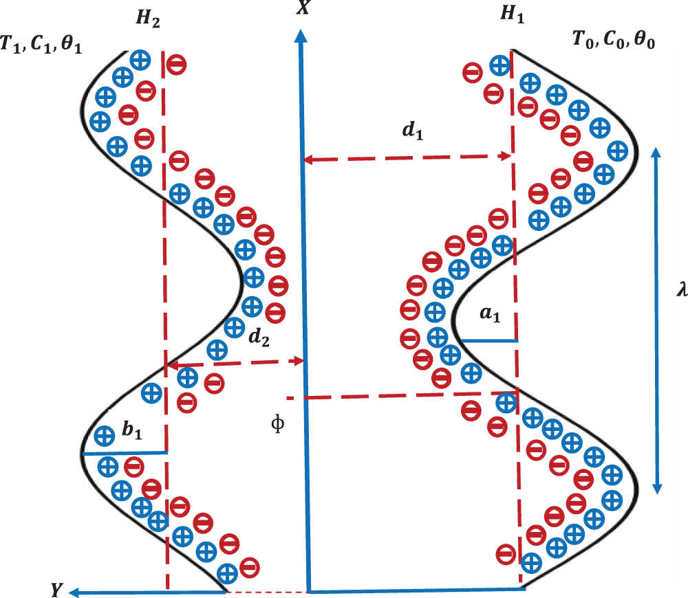
Figure 1: Geometry of the problem

In the equations displayed earlier a1 and b1 signify the oscillation amplitudes, λ is defined as the wavelength and t indicates the time period.

When double diffusion, viscous dissipation and radioactive heat flux are considered, the heat energy, nanoparticle proportion, and solute concentration of solute are described as [41–43].

∇⋅V=0(6)

ρf(dVdt)=∇⋅τ+μe(A+⋅∇)A+−∇(12μe(A+)2)+ρeE+g(ρf0(1−Θ0)(βT(T−T0)+(C−C0)βC)−(ρp−ρf0)(Θ−Θ0))(7)

(ρc)f(dTdt)=k∇2T+(ρc)p(DB(∇Θ⋅∇T)+(DTT0)(∇T)2)+S⋅L−∇⋅qr+DTC∇2C+σ(E⋅E)(8)

dCdt=Ds∇2C+DCT∇2T(9)

dΘdt=DB∇2Θ+(DTT0)∇2T(10)

The term qr defined in Eq. (8) is the flow of thermal radiations (solar energy) and is determined by implementing the Rosseland mean diffusion approach as [41].

qr=−4σ∗3k∗∂T4∂Y(11)

By eliminating the higher powers of T in the taylor series of T4, we get differntial form of Eq. (11) as:

∂qr∂Y=−16σ∗T033k∗∂2T∂Y2(12)

where k∗ symbolizes for Rosseland mean absorptivity and σ∗ refers to Stefan’s constant.

3.1 Electroosmotic Phenomenon

The description of the Poisson equation in a channel that is asymmetric is [38].

∇2ω=−ρeε(13)

here ε,ω and ρe are dielectric permittivity, electric potential and net charge density, respectively.

The electric charge density ρe ensures the Boltzmann factor, in case as:

ρe=ez(n+−n−)(14)

where z,e,n+ and n− represent the charge neutrality, the electronic charge, positive ions, and ionized anions. After simplifaction, we get:

ρe=−2zen0(ezωkBTv)(15)

where n0 represent the bulk concentration, the Boltzmann constant is denoted by kB and Tv signifies total temperature. By putting on Debye-Huckel estimation, the Eq. (13) becomes:

d2ωdy2=f2ω(16)

with boundary conditions [38]:

ω=0,at y=h1(17)

ω=1,at y=h2(18)

The exact solution to Eq. (16) subject to boundary constraints (17) and (18) becomes:

ω(y)=sinh⁡(f(y−h1))sinh⁡(f(h2−h1))(19)

3.2 Translation and Scaling of Variables

The component forms of Eqs. (10)–(14) are given as follows [41]:

∂U∂X+∂V∂Y=0(20)

ρf(∂U∂t+U∂U∂X+V∂U∂Y)=−∂P∂X+∂SXX∂X+∂SXY∂Y−μe2(∂A+2∂X)+μe(aX∂aX∂X+aY∂aX∂Y+A0∂aX∂Y)+ρeEX+g(ρf0(1−Θ0)(βT(T−T0)+(C−C0)βC)−(ρp−ρf0)(Θ−Θ0))(21)

ρf(∂V∂t+U∂V∂X+V∂V∂Y)=−∂P∂Y+∂SYX∂X+∂SYY∂Y−μe2(∂A+2∂Y)+μe(aX∂aY∂X+aY∂aY∂Y+A0∂aY∂Y)(22)

(ρc)f(∂T∂t+U∂T∂X+V∂T∂Y)=k(∂2T∂X2+∂2T∂Y2)+(ρc)p(DB(∂Θ∂X∂T∂X+∂Θ∂Y∂T∂Y)+(DTT0)((∂T∂X)2+(∂T∂Y)2))+(SXX∂U∂X+SXY(∂U∂Y+∂V∂X)+SYY∂V∂Y)+16σ∗T033k∗(∂2T∂X2+∂2T∂Y2)+DTC(∂2C∂X2+∂2C∂Y2)+σEX2(23)

∂C∂t+U∂C∂X+V∂C∂Y=Ds(∂2C∂X2+∂2C∂Y2)+DCT(∂2T∂X2+∂2T∂Y2)(24)

∂Θ∂t+U∂Θ∂X+V∂Θ∂Y=DB(∂2Θ∂X2+∂2Θ∂Y2)+(DTT0)(∂2T∂X2+∂2T∂Y2)(25)

where SXX,SXY, and SYY represent Sisko fluid stresses in elementary form. To convert an unstable flow field into a steady wave frame of reference, Galilean transformations is applied under shifting and scaling strategies. The Galilean transformation in conjunction with two reference frames is represented by:

u=U−c,y=Y,x=X−ct,p(x,y)=P(X,Y,t),v=V(26)

Dimensionless transformations are defined as below [30,43].

x¯=xλ,y¯=yd1,v¯=vc,u¯=uc,δ=d1λ,t¯=ctλ,Re=ρfcd1μ,d=d2d1,a=a1d1,b2=b1d1,h¯1=H1d1,h¯2=H2d1,θ=T−T0T1−T0,Ω=Θ−Θ0Θ1−Θ0, v¯=−δ∂ψ∂x¯,u¯=∂ψ∂y¯,ax=∂ξ∂y,ay=−δ∂ξ∂x,Rd=16σ∗T033k∗μcf,Ln=νDB,Le=νDS,γ=C−C0C1−C0,p¯=d12cμλp(27)

In view of Eqs. (26) and (27) and applying the long wavelength constraint (δ ≪ 1), Eqs. (20)–(25) are simplified (with fnite Reynolds number) [44].

dpdx=∂Sxy∂y+ReS12ξyy+Grtθ+Grcγ−GrFΩ+Uhsωyy(28)

0=∂2θ∂y2+NTCPr∂2γ∂y2+NbPr(∂θ∂y∂Ω∂y)+NtPr(∂θ∂y)2+RdPr∂2θ∂y2+Br(∂2ψ∂y2)(∂2ψ∂y2+m∗(∂2ψ∂y2)b)+Prβ(29)

∂2γ∂y2+NCT∂2θ∂y2=0(30)

∂2Ω∂y2+NtNb∂2θ∂y2=0(31)

ξyy=Rm(E−∂ψ∂y)(32)

where

Sxy=(1+m∗((∂2ψ∂y2)2)b−12)∂2ψ∂y2(33)

The dimensionless stresses are composed as:

Sxy=(1+m∗((∂2ψ∂y2)2)b−12)∂2ψ∂y2(34)

In non-dimensional form, the Eqs. (4) and (5) give:

y=h1=1+acos⁡(2πx)(35)

y=h2=−d−bcos⁡((2πx)+ϕ)(36)

After eliminating pressure term from Eq. (28) and using Eq. (34), we receive:

∂2∂y2((1+m∗((∂2ψ∂y2)2)b−12)∂2ψ∂y2)−M2∂2ψ∂y2+Grt∂θ∂y+Grc∂γ∂y−GrF∂Ω∂y+Uhs∂3ω∂y3=0(37)

The corresponding boundary conditions for an asymmetric channel have the following non-dimensional form [36–38].

ψ=F2,∂ψ∂y=−1ony=h1 and ψ=−F2,∂ψ∂y=−1ony=h2(γ,θ,Ω=0ony=h1) and (γ,θ,Ω=1ony=h2),ξ=0ony=h1 andy=h2.(38)

where F represents the time average wave frame flow rate.

4  Solution of the Problem

As we can see that the obtained mathematical relations are highly nonlinear and mutually dependent which cannot be perfectly handled by typical analytical or numerical methods. In this regard, the Morlet Wavelet Neural Networks (MWNNs) play an essential role in the attainment of greater accuracy and efficiency in neural network-based solutions to complex mathematical models. In comparison with traditional activation functions, the Morlet wavelet possesses the advantage of improved localization in time and frequency domains, which enables MWNNs to capture intricate patterns and dynamic behavior effectively. This renders them extremely well-suited for the solution of differential equations, signal processing, and engineering applications. MWNNs also improve convergence rates and reduce computational errors when paired with optimization methods like Particle Swarm Optimization (PSO). Their flexibility and accuracy also render them an effective tool in scientific computing and artificial intelligence applications. Fig. 2 demonstrates the framework of the considered Artificial Neural Netwroks (ANN) model.

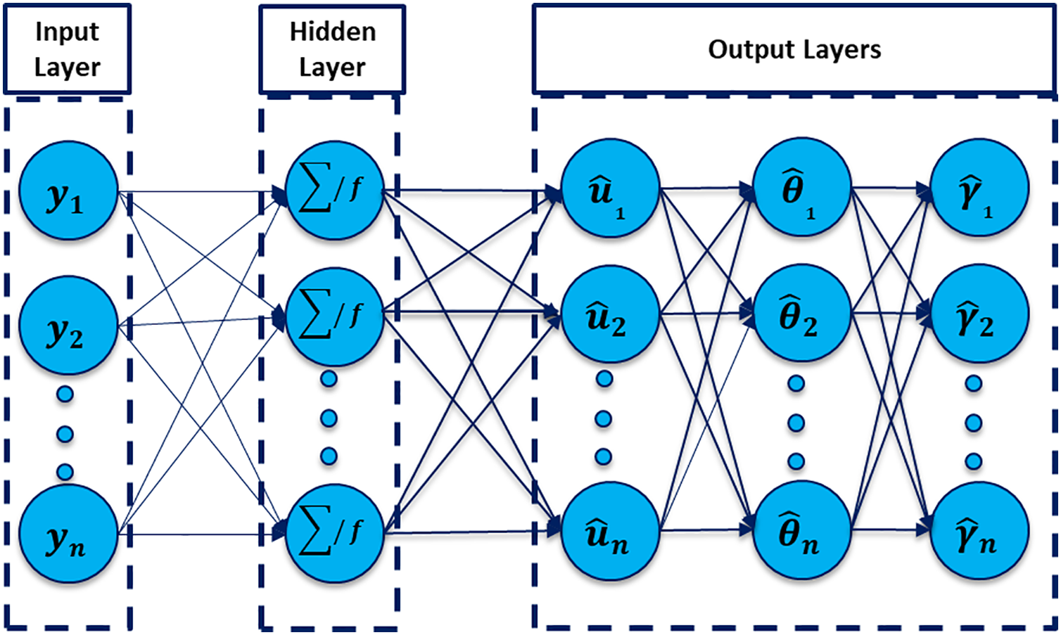
Figure 2: Design of the ANNs architecture

4.1 Morlet-Wavelet Neural Networks Methodology (MWNNs)

The Morlet Wavelet Neural Networks (MWNNs) combined with Particle Swarm Optimization (PSO) and Neural Network algorithm (NNA) follows methodical approach in arriving at the optimal solutions in Fig. 3. The key steps are:

I.   Problem Formulation: Determine the governing equations and transform them into a suitable mathematical formulation.

II.   MWNNs Initialization: Formulate the neural network with Morlet wavelet activation functions. Initialize weight and bias matrices for MWNNs.

III.   Optimization Using PSO: Initialize a population of particles comprising weights and biases. Particle positions and velocities are updated using the best local and global solutions.

IV.   Optimize MWNN parameters iteratively to minimize the error function.

V.   Neural Network Architecture (NNA): Enhancement Use bias and weight adjustment operators to enhance solutions.

VI.   Solution Evaluation & Stopping Criteria: Compute error metrics like Mean Squared Error (MSE) and Theil’s Inequality Coefficient (TIC) to assess model accuracy. If the convergence criteria are met, finalize the solution; otherwise, proceed with iterations.

VII.   Result Validation & Interpretation: Compare the results between the proposed methodology with NDsolve through statistical analysis.

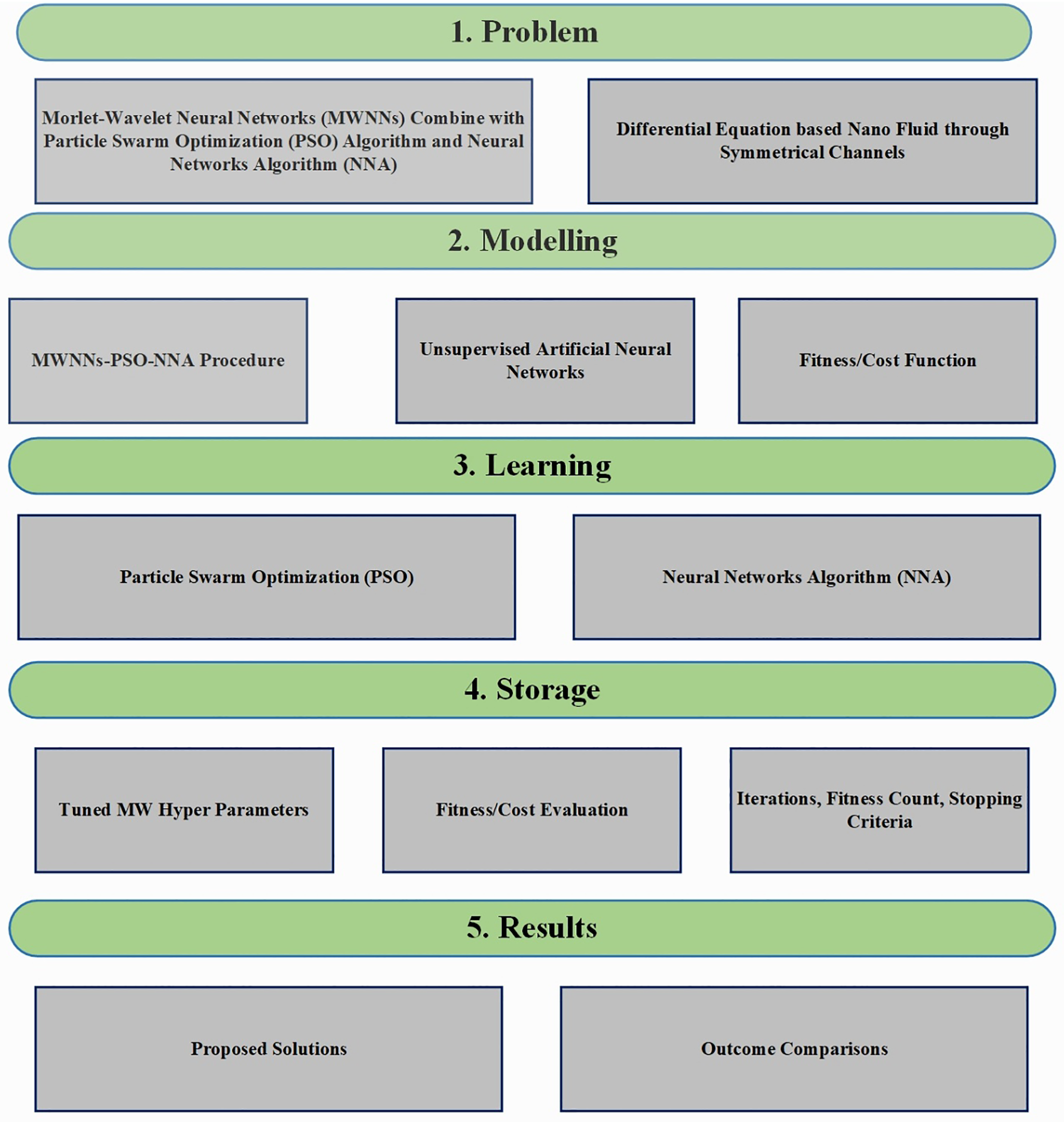
Figure 3: Design methodology through MWNNs

4.2 Mathematical Formulation for Morlet Wavelet Neural Networks

To address the non-Newtonian Sisko fluid containing suspended nanoparticles in asymmetric channels using MWNNs, the obtained solution is denoted as S^(v), where S^n(v) represents the nth derivative, defined as follows:

S^(v)=∑i=1tσiG(ρiy+τi),

S^n(v)=∑i=1tσiGn(ρiy+τi),

where t represents neurons and [ρui,τui,σui,ρθi,τθi,σθiργi,τγi,σγi], shows the components (weights and biases) for the velocity function, temperature distribution and concentration. The MW function is N(z)=cos⁡(1.75z)(e−0.5z2) is expressed into MW neural networks according to the following velocity function, temperature distribution, and concentration:

u^(y)=∑i=1oσui[e−0.5(τui+ρuiy)2Cos[1.75(τui+ρuiy)]](39)

θ^(y)=∑i=1oσθi[e−0.5(τθi+ρθiy)2Cos[1.75(τθi+ρθiy)]](40)

γ^(y)=∑i=1oσγi[e−0.5(τγi+ργiy)2Cos[1.75(τγi+ργiy)]](41)

The MW neural networks based fitness functions are given in Appendix A.

4.3 Meta-Heuristic Global Optimization Algorithms

The algorithms used in metaheuristic optimization are powerful computational techniques that find near-optimal solutions for complex problems where traditional optimization algorithms may fail. A few of them, like Particle Swarm Optimization (PSO), Genetic Algorithms (GA), and Water Cycle Algorithm (WCA), are popularly used to optimize the weights and biases of Morlet Wavelet Neural Networks (MWNNs). The significance of metaheuristic optimization in MWNNs is its ability to efficiently search high-dimensional spaces, avoid local minima, and enhance the accuracy and generalization of the network. By optimizing the weights of MWNNs, these algorithms improve the network’s ability to model and solve nonlinear differential equations, fluid dynamics, and other complex mathematical problems, which makes them very valuable in engineering and scientific applications.

4.4 Particle Swarm Optimization

The population-based metaheuristic optimization technique known as Particle Swarm Optimization (PSO) was motivated by the social behavior of fish schools and bird flocks. In order to improve candidate solutions iteratively through collaboration and self-adaptation, Kennedy and Eberhart [45] proposed it. Every particle in the swarm functions as a possible solution and uses both its own and neighboring particles’ experiences to update its location in the search space. PSO has been effective in a variety of domains, including machine learning for optimizing neural network weights, engineering design for optimizing structures, biomedical research for processing medical images, finance for predicting stock markets, and computational fluid dynamics for solving nonlinear equations [46,47]. Its effectiveness, simplicity, and ability in solving high-dimensional optimization problems have made PSO a commonly used method in numerous scientific and engineering fields [48–52].

Particle Velocity Update:

Yix=wYit−1+c1r1(PLBx−1−Zix−1)+c2r2(PGBx−1−Zix−1)

Particle Position Update:

Zix=Zix−1+Yix−1

In this case, w represents the inertia weight that strikes a balance between local exploitation and global exploration. While r1 and r2 are random values uniformly distributed in the interval [0, 1], c1 and c2 are the cognitive and social acceleration coefficients, respectively.

4.5 Neural Networks Algorithm

Introducing a new version of the NNA74, artificial neural networks (ANNs) and organic nerve systems serve as inspiration for the new evolution strategy. Although ANNs are primarily used for predictive modeling, the NNA is distinct in integrating principles of neural networks with stochastic mechanisms to efficiently resolve optimization challenges. Leveraging the internal computational structure of neural networks, NNA boasts strong global search capability, enhancing optimization effectiveness. Notably, it varies from other conventional metaheuristic algorithms in that its behavior is exclusively influenced by the population size and termination criteria, without any other algorithmic parameters. As a population-based optimization technique, NNA is designed around four crucial components.

4.6 Update Population

In the NNA framework, the population at Mth iteration is denoted as Yt={y1t,y2t,y3t,…,yMt} which evolves through the weight matrix Wt={w1t,w2t,w3t,…,wMt}. Here, the weight matrix for the ith individual is denoted as wti={wi,1t,wi,2t,wi,3t,…,wi,Mt} while the ith individual’s position is provided by yti={yi,1t,yi,2t,yi,3t,…,yi,Et}. The mathematical representation of the updated population is formulated as follows:

ynew,jt=∑j=1Mwj,kt×yjt,k=1,2,3,…,M

yjt=yjt+ynew,jt,j=1,2,3,…,M

The population size is assigned accordingly, t being the number of iterations. The weight vector is represented in the following manner.

∑j=1Mwj,kt=1,0<wj,kt<1

4.7 Update Weight Matrix and Bias Operator

The weight matrix W is essential in Neural Network Architectures (NNA) for generating new populations, following the update rule:

wjt=|wit+2×λ2(wobjt−wjt)|,j=1,2,3,…,M

where λ2, and wobjt are the objective weight matrix. The bias operator enhances network adaptability, with its parameter β1 updated as β1t+1=0.99β1t.

Bias components Mp and Mw are determined as Mp = β1t×E and Mw=[β1t×M], randomly selecting elements from defined ranges. The bias population and weight matrices are given by:

yj,P(S)t=lP(S)t+(uP(S)−lP(S))×λ3,S=1,2,3,…,MP

where λ3,λ4∈[0,1].

4.8 Transfer Operator

The main objective of the NNA optimization method is to enhance the optimal solution to be equal to the current exact solution through the local best search property of NNA. Mathematically, this is stated as follows:

yjt+1=xjt+2λ5(yobjt−yjt),j=1,2,3,…,M

where λ5 is uniformly distributed within the domain [0,1] similar to other global enhancement techniques, the NNA method begins with the following expression:

yj,kt=lk+(uk−lk)×λ6,j=1,2,3,…,M,k=1,2,3,…,E

where λ6 denotes a random value drawn from the interval [0,1].

5  Results and Discussion

Artificial neural networks with a Morlet wavelet nonlinear activation function are employed to address the problem and to achieve higher accuracy than typical numerical methods. Morlet-Wavelet Neural Networks (MWNNs) are important to capture intricate nonlinear structures because they are capable to integrate wavelet transforms with learning through neural networks. The fact that they are localized oscillatory improves the approximation to functions, making them very efficient to use in solving differential equations and scientific computation. The design methodology step by step is represented in Fig. 3, the fitness function in Fig. 4a indicates the convergence behavior during different independent runs, establishing the stability and efficiency of the optimization process. The Fig. 4b,c of the TIC and MSE indicates the behavior of the Theil’s Inequality Coefficient and Mean Squared Error, showing the predictive accuracy of the model during across multiple runs. The boxplot of the MSE values during independent runs in Fig. 4d compares the values, showing the robustness and variance of the model. The boxplot of the TIC during independent runs in Fig. 4e further indicates the reliability of the solution. The Fig. 4f of the normal distribution of the MSE indicates the statistical distribution of the errors, establishing the stability of the performance and the normality assumption. In Fig. 4g of the normal distribution of the TIC provides further analysis of the behavior of the predictive error. The graphical analysis collectively indicates the reliability of the model during different independent runs. The final results represent that the optimization process has stability while providing minimum variance to the measures of the error. This extensive statistical evidence proves the efficacy of the proposed neural network technique to the given problem. The proposed framework advances existing methods by providing higher accuracy and faster convergence chatcompared to classical numerical techniques. Its efficiency makes it suitable for solving complex nonlinear fluid flow models that are otherwise challenging with traditional methods.

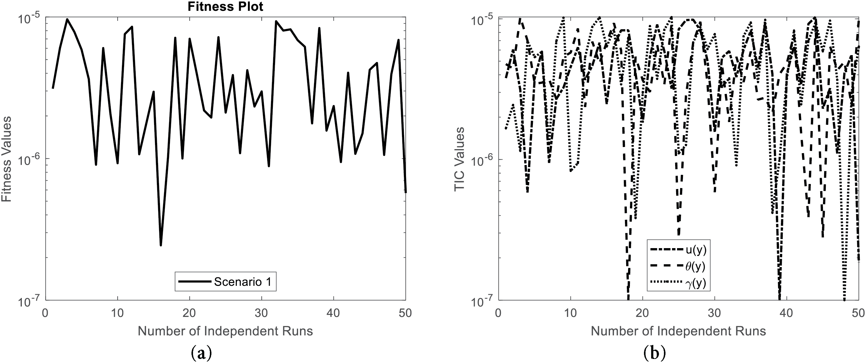
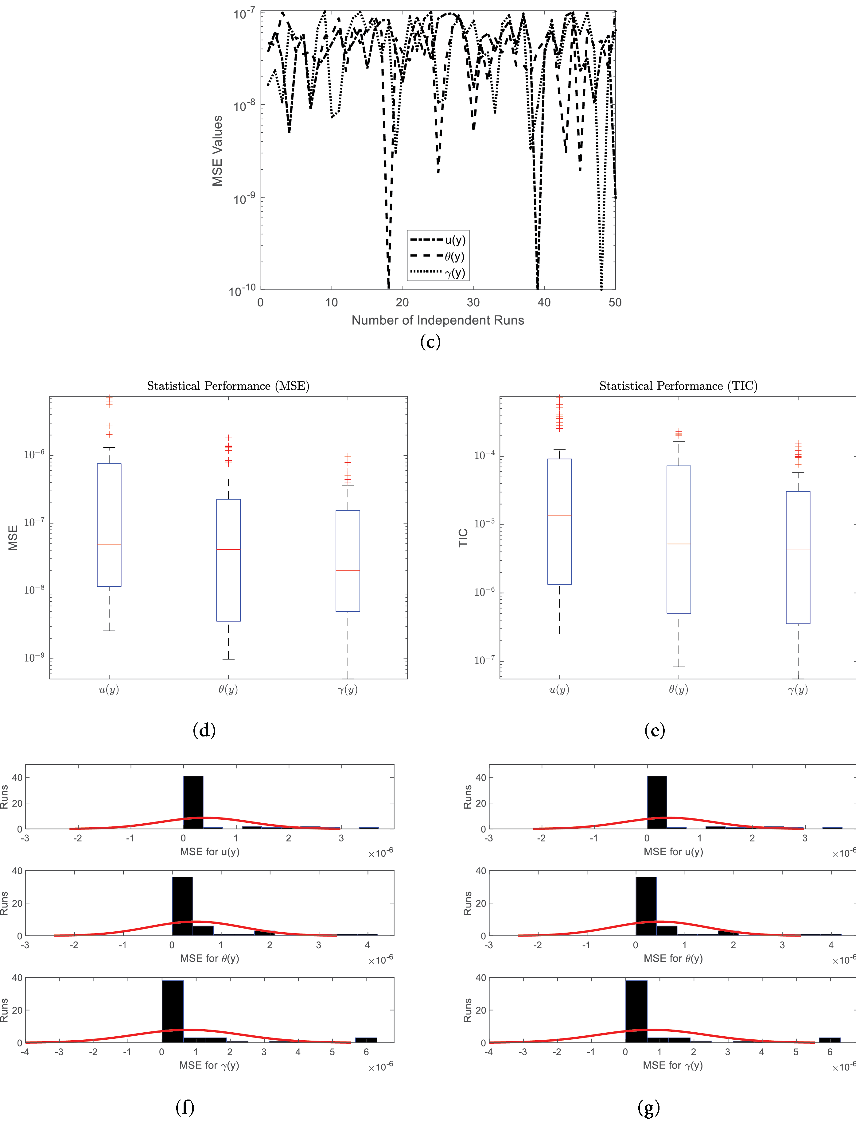
Figure 4: Convergence analysis through fitness, MSE and TIC

The integrated MWNNs-PSO-NNA program is used in MATLAB to solve the equations, and the MWNNs-PSO-NNA command is utilized for nonlinear expressions. MWNNs-PSO-NNA, which is essentially A function in Wolfram Language, can solve differential equations in numerical form and a variety of partial derivatives as well as initial value problems. Within this segment, many variables that influence the velocity curve, isotherm distribution, concentration gradient, nanoparticle volume fraction, Lorentz force function, gradient of fluid pressure, and pressure escalation rate profile are displayed in Figs. 5–16.

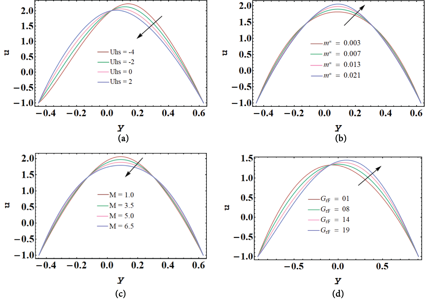
Figure 5: Velocity profile affected by Uhs,m∗,M and GrF

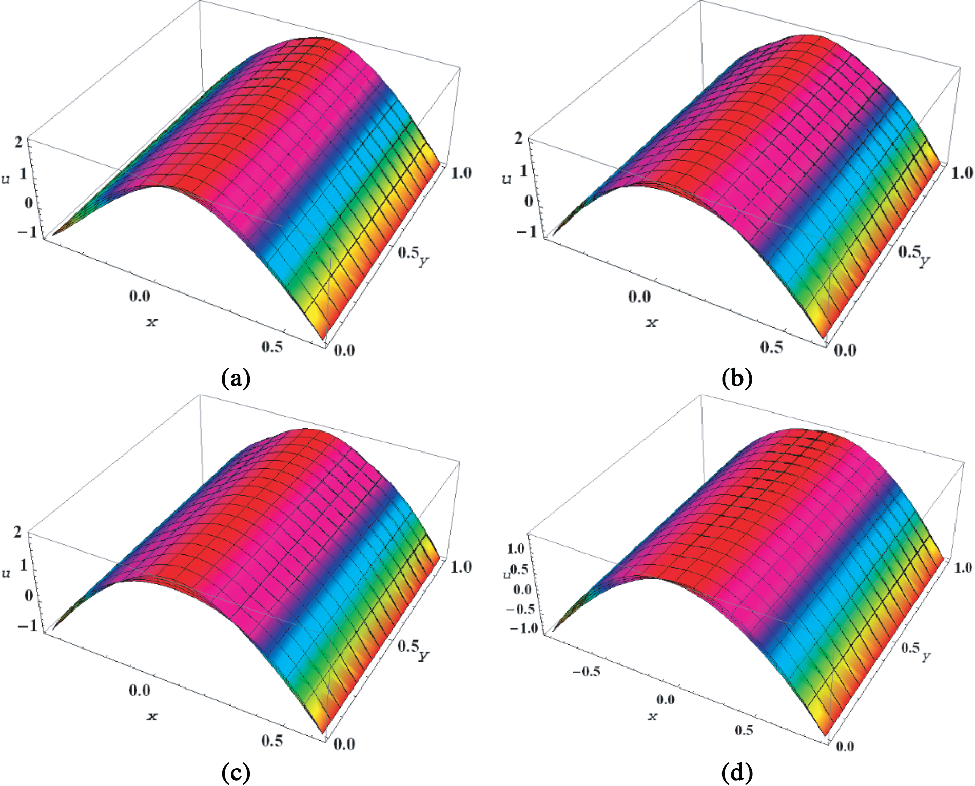
Figure 6: Velocity profile for Uhs,m∗,M and GrF within three coordinate system

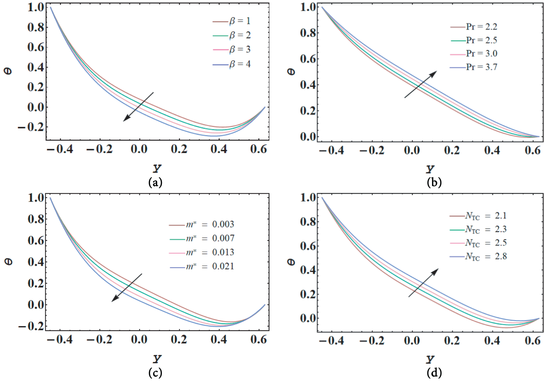
Figure 7: Temperature profile for β,Pr,m∗ and NTC

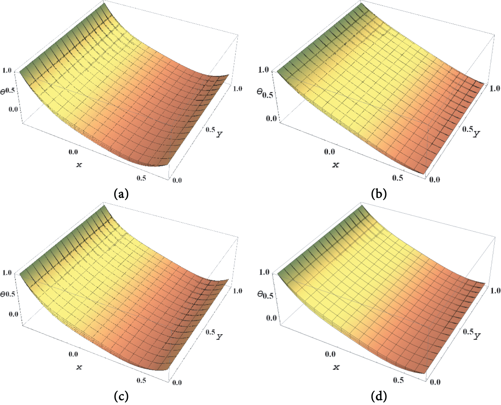
Figure 8: Temperature profile for β,Pr,m∗ and NTC within three coordinate system

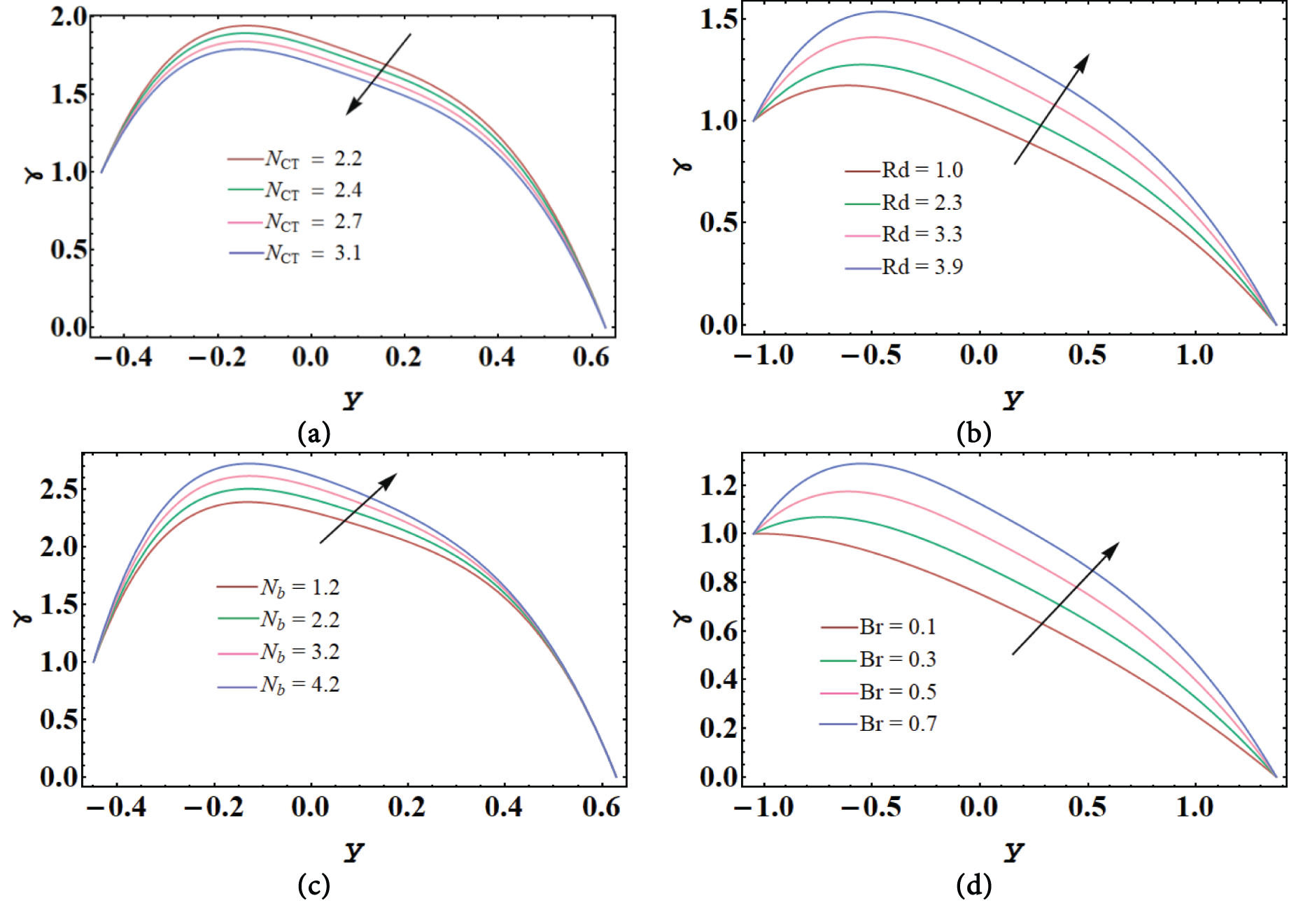
Figure 9: Concentration profile for NCT,Rd,Nb and Br

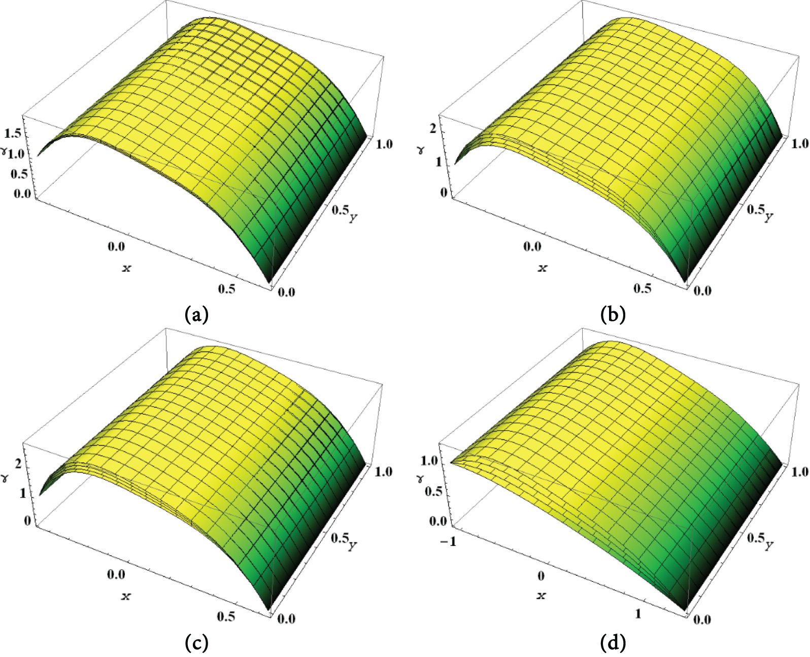
Figure 10: Concentration profile for NCT,Rd,Nb and Br within three coordinate system

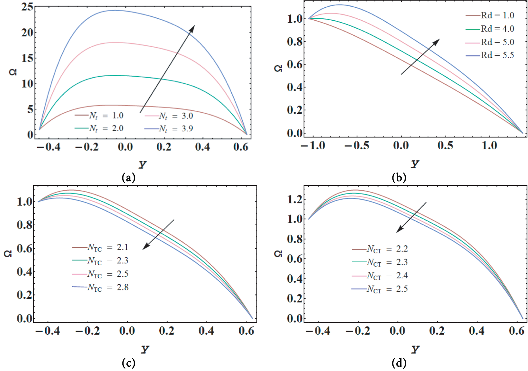
Figure 11: Nanoparticle volume fraction for Nt,Rd,NTC and NCT.

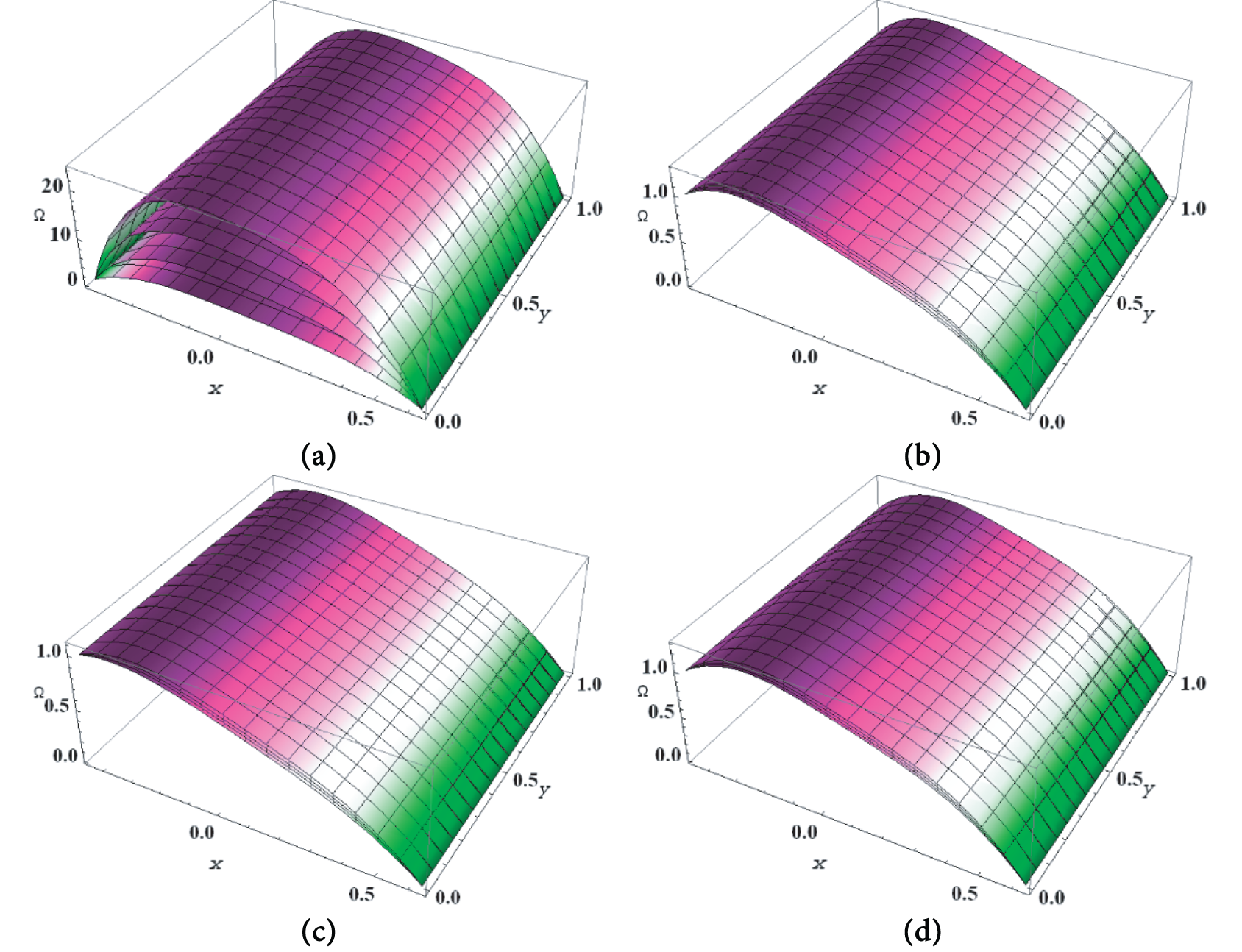
Figure 12: Nanoparticle volume fraction for Nt,Rd,NTC and NCT within three coordinate system

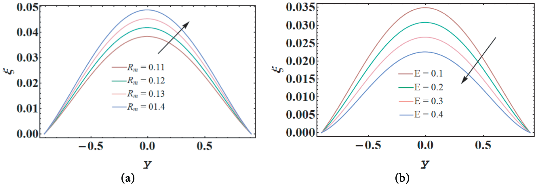
Figure 13: Magnetic force function under the impact of Rm and E

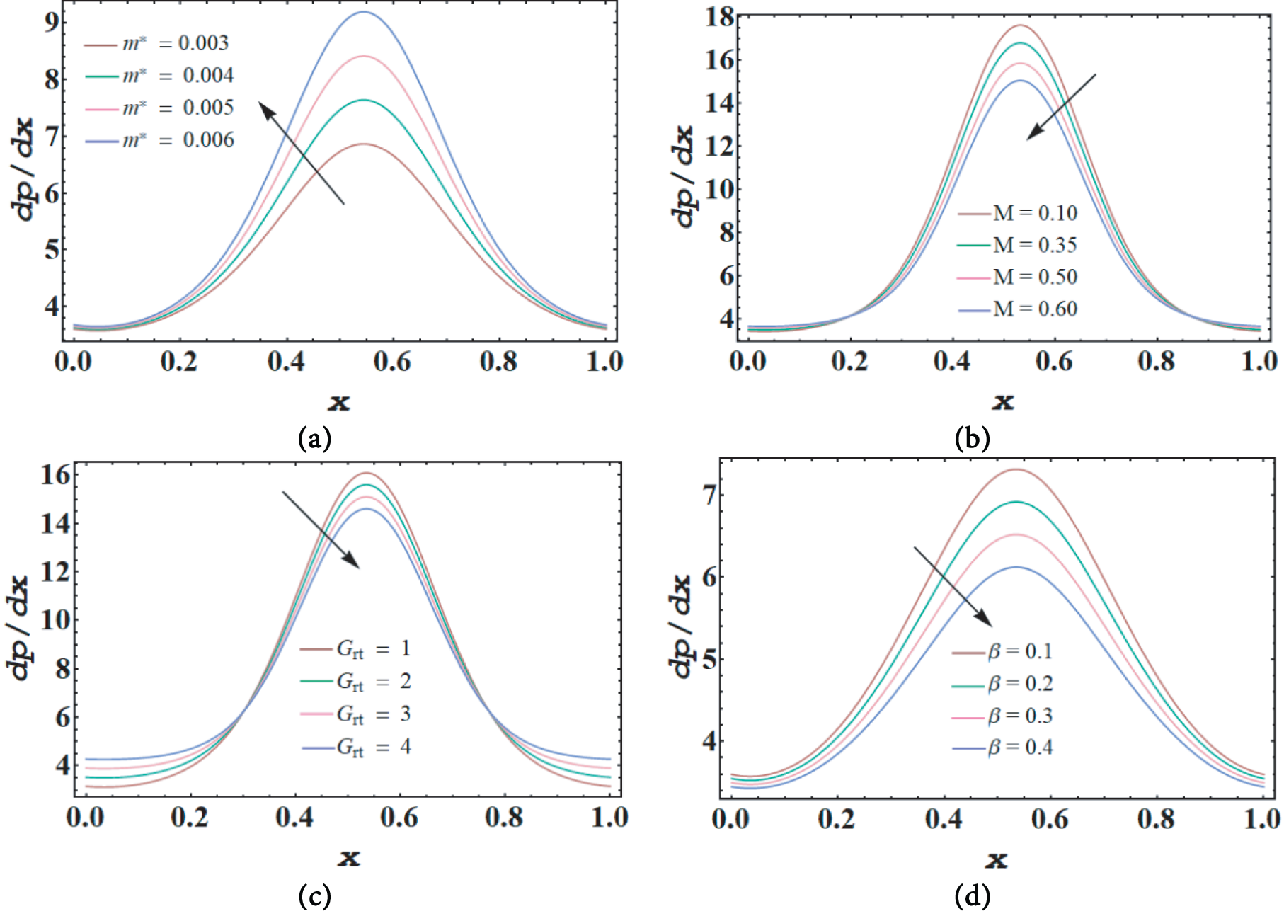
Figure 14: Pressure gradient profile affected by m∗,M,Grt and β

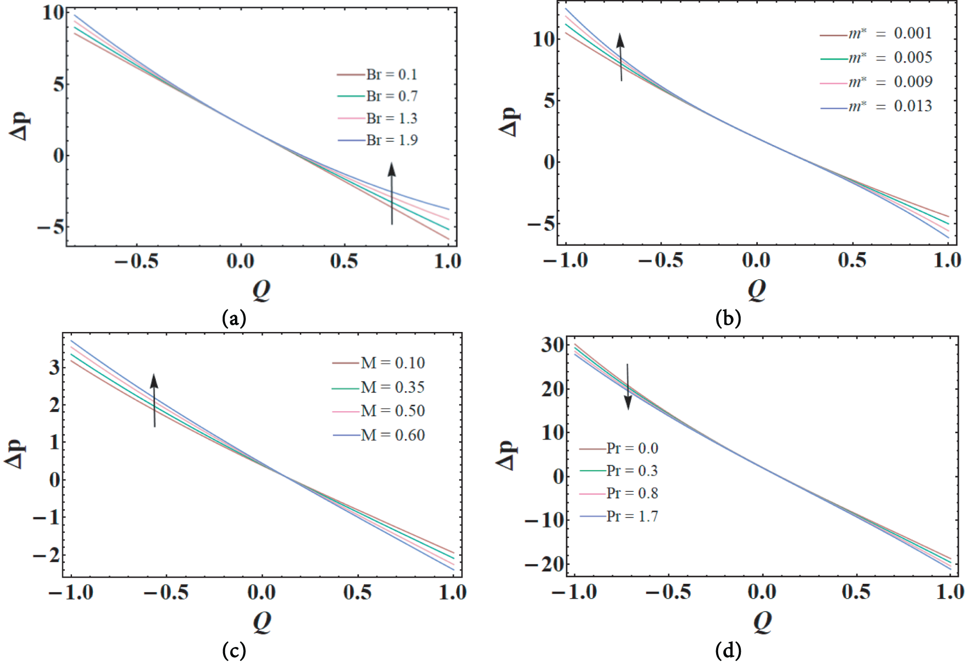
Figure 15: Pressure rise affected by Br,m∗,M and Pr

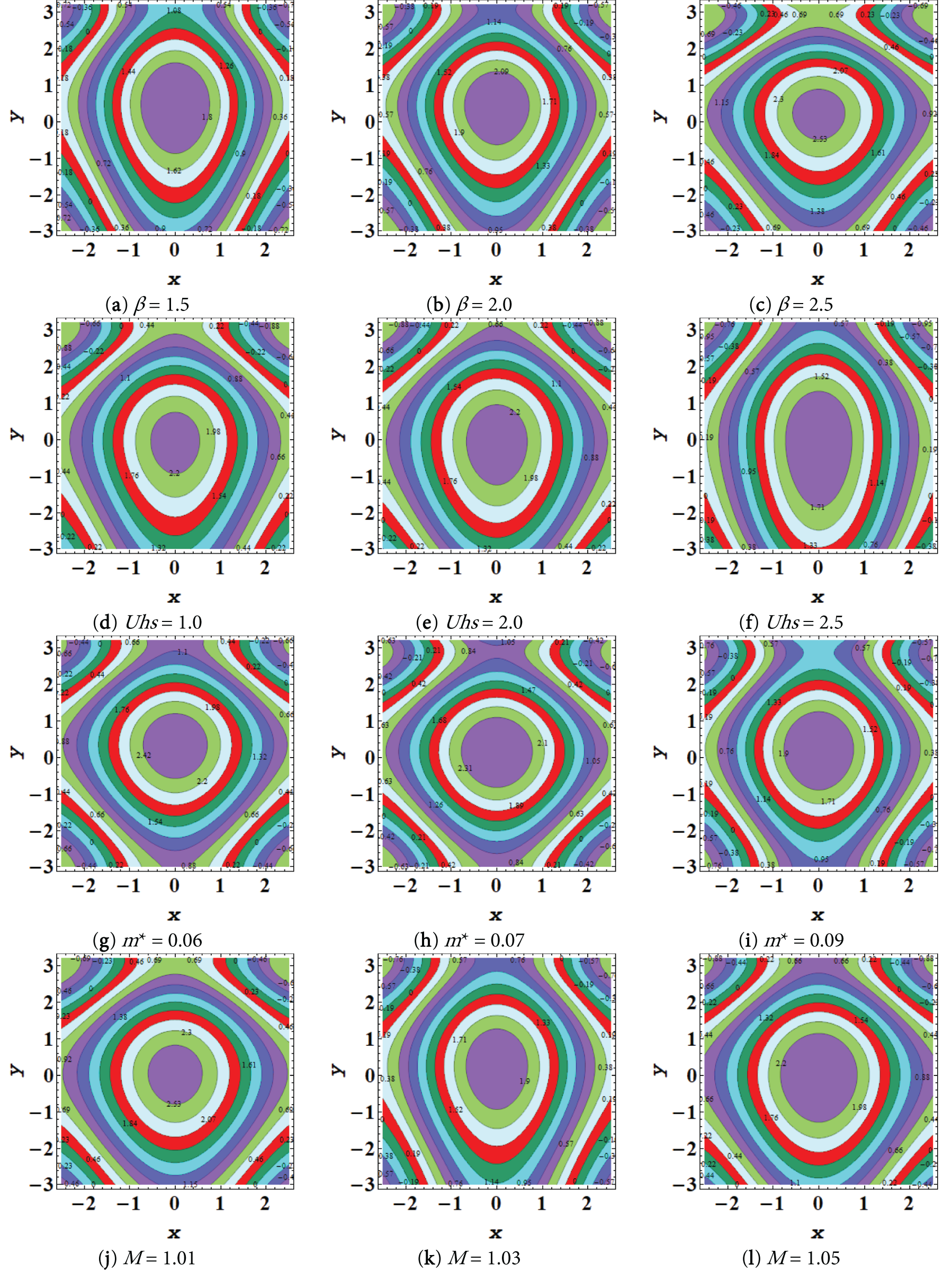
Figure 16: Impact of β,Uhs,m∗ and M on streamline

Using different values of the Helmholtz-Smoluchowski velocity (Uhs), Hartmann number (M), Sisko parameter (m∗) and dimensionless nanoparticle Grashof number (GrF), Fig. 5a–d examines the phenomenon of flow velocity. As presented in Fig. 5a, fluid velocity has a tendency to increase when embedded in zone y∈[−0.45,0.1] that represents a surface velocity or driving force that actively accelerates the fluid and decreases when it is in the sector y∈[0.1,0.63] because of the growing influence of Uhs. According to Fig. 5b, due to enhanced resistance, the velocity profile dropped in the interval y∈[−0.45,−0.1] and y∈[0.3,0.63], while it grew in the region y∈[−0.1,0.3] where the predominant shear-thinning effects lower flow resistance as a result of the increasing m∗. The velocity profile in Fig. 5c improves within the regions y∈[−0.45,−0.1] and y∈[0.3,0.63], while decreasing in the region y∈[−0.1,0.3] as a result of the increasing M because motion is opposed by powerful Lorentz forces. However, it is important to note that the magnetic field does not always act as a retarding effect; in certain flow configurations it may assist the motion, as stated in [53]. The velocity falls in the region y∈[−0.9,−0.1] due to opposing effects and rises in the region y∈[−0.1,0.9]as mobility is improved in that area when buoyancy matches the direction of flow when the GrF value increases, as shown graphically in Fig. 5d. It can also be observed that this velocity is much greater than that of measured in [41]. The reason for this increase is that in the current study, electroosmosis (which was not in [43]) is creating an acceleration to the flow velocity, as in the presence of this effect, the electric body force becomes stronger enhancing the fluid motion. Fig. 6a–d shows 3D velocity profiles that behave similarly to the 2D velocity profiles. A more thorough picture is offered by the 3D graphs, which draw attention to the spatial differences and the consistency of the trends shown in the 2D graphs. While highlighting the complexity of 3D modeling for comprehending velocity distributions in intricate flow systems, this resemblance highlights the dependability of the 2D analysis and provides improved clarity for interpreting physical occurrences.

Fig. 7a–d shows how temperature distribution affects the non-Newtonian parameter (m∗), Dufour parameter (NTC), the parameter for Joule heating (β) and also Prandtl number (Pr). As the values of β increase, it is clear from Fig. 7a indicates that the pattern of temperature declines due to the fact that more heat is effectively transferred or conveyed. This finding aids in electroosmotic pumps, microelectromechanical systems (MEMS), and microchip cooling, where effective heat removal reduces overheating and boosts device dependability. The concentration distribution in Fig. 7b is increased by a greater Pr, showing that the diffusion of species is slowed by lower molecular diffusivity in comparison to momentum diffusivity. This observation is pertinent to the design of heat exchangers, lubrication systems, and nanofluid thermal management. The effects of m∗ and NTC on concentration distribution are represented in Fig. 7c,d. As the value of m∗ grows, non-Newtonian effects increase resistance, reducing fluid volume in the channel as shown in Fig. 7c and as NTC increases, which improves thermal-diffusion coupling, which intensifies thermophoretic effects and promotes larger concentration gradients and concentration distribution in Fig. 7d. This result for the Sisko fluid factor will be beneficial for regulating rheological behavior, which regulates flow homogeneity and cooling rates in polymer manufacturing, biofluids, and slurry transport. Impact of NTC remains crucial for heat exchangers based on nanofluids, fuel cells, and chemical reactors, where reaction efficiency is impacted by thermal–mass coupling. Furthermore, temperature distribution is enhanced due to additional radiative heat flux, which contributes to the overall energy transport; however, excessively strong radiation effects may reduce the accuracy of linearization assumptions, so the chosen range balances practicality with numerical stability. Fig. 8a–d processes 3D thermal distribution profiles that perform equivalent to the 2D profiles. By more accurately depicting spatial changes, validating the designs seen in the 2D graphs, and offering a more thorough comprehension of the thermal behavior, the 3D representation improves visualization.

The features of solutal concentration are shown in Fig. 9a–d on Soret constraint (NCT), Thermal radiation (Rd), Brownian motion (Nb) and Brinkman number (Br). Fig. 9a presents the findings on the Soret parameter NCT. The concentration profile falls when the NCT increases because a larger NCT upsurges the thermal diffusion effect, which causes particles to move from hotter to colder locations. Because of this redistribution, the concentration profile generally declines since there is less particle accumulation in the primary concentration zone. As discussed in the Fig. 9b–d, the concentration profile boosts consequent to the rise in Rd,Nb and Br. Physically, a higher Rd increases the system’s thermal radiation, which raises the temperature and encourages more robust particle diffusion, both of which increase the concentration. A greater Nb denotes improved dispersion due to intensified Brownian motion, in which nanoparticles collide randomly. In a similar vein, a higher Br value denotes stronger thermophoretic forces, which push particles from hotter to cooler areas and enhance accumulation. When combined, these actions cause the concentration profile to rise. Consistent with the 2D plots, the 3D solutal concentration profiles shown in Fig. 10a–d show that the solutal concentration decreases in response to increasing distance from the surface. In addition to verifying the trends seen in the 2D profiles, the 3D representation offers a more thorough picture of spatial variations and a more profound understanding of concentration distribution patterns.

Fig. 11a–d illustrates how the volume fraction of nanoparticles influences a number of fluid properties, including thermophoresis parameter (Nt), Thermal radiation (Rd), Dufour parameter (NTC) and Soret parameter (NCT). The movement of nanoparticles caused by temperature gradients intensifies with increasing Nt leading to the accumulation of nanoparticles in particular areas. Because increased thermophoretic processes drive particle motion, the fluid’s nanoparticle volume fraction rises in the way shown in Fig. 11a. Fig. 11b shows the effect of Rd on the nanoparticle profile. Improving thermal radiation raises the system’s energy content, which encourages thermally driven diffusion and particle motion. This intensifies thermal effects, which elevates the nanoparticle profile. On the other hand, NTC and NCT produce adverse consequences because they promote diffusion mechanisms that hinder the formation process, which lowers the concentration of nanoparticles in certain areas, as shown in Fig. 11c,d. The nanostructure 3D volume fragment profiles in Fig. 12a–d show patterns resembling those in the 2D graphs, with the volume fraction falling with increasing distance from the surface. The 3D display successfully draws attention to spatial changes, enhancing the coherence of the 2D analysis and offering a better understanding of nanoparticle configuration.

One of the fundamental cosmic powers, the magnetic force is produced by the dynamic movement of charges and is induced by the electromagnetic force. Moreover, when two charged items get close to one another, a magnetic attraction force is produced. The magnetic Reynolds number affects the correlative influence of the magnetic force (Rm) and electrical field (E) is depicted in Fig. 13a,b. As the magnetic Reynolds number increases, Fig. 13a below illustrates that the function of magnetic force often rises as well, suggesting that the influence of electromagnetic induction on fluid behavior is growing in significance. In Fig. 13b, increases in electric field intensity cause the charged fluid particles to accelerate, negating the constraining effect of the magnetic force and lowering the magnetic force function profile.

Fig. 14a–d shows how the pressure differential dpdx alongside the x direction is affected by the non-Newtonian parameter (m∗), Hartmann dimensionless parameter (M), Grashof number for thermal convection (Grt) and Joule heating parameter (β). The pressure gradient rises as the m∗ increases as evident from Fig. 14a. This implies that there is more resistance or slower fluid movement across the medium when m∗ is larger. Density or flow path alterations could be the cause of this. Whereas Fig. 14d shows the opposite effects, ultimately as a result of more direct or smoother channels, suggesting a faster flow and less resistance. The pressure gradient profile in Fig. 14b improves in the domains x∈[0.0,0.2] and x∈[0.85,1.0] as a result of the increasing M due to improved flow conditions or lower resistance, while it falls in the region x∈[0.2,0.85]. As shown in Fig. 14c, the pressure gradient rises across the regions x∈[0.0,0.3] and x∈[0.75,1.0] and falls in the region x∈[0.3,0.75] by increasing Grt which indicates less resistance or a more effective flow, perhaps as a result of smoother channels or less friction.

As seen in Fig. 15a–d, the impact of numerous factors on the pressure rise per cycle Δp plotted vs. flow rate Q. The pumped phases are divided into consecutive sections in order to highlight almost all the aspects of pressure rise. a) The region undergoes peristalsis when Q>0 and Δp>0: Pressure in this area is frequently modulated by peristalsis waves, which move fluid in the direction of the flow process. b) The augmented region persists when Q>0 and Δp<0: The flow is improved in this region by the pressure created by the peristaltic force. c) The retrograde area resides when Q<0 and Δp>0: Due to peristalsis compression impedes the flow in this region, pressure rises in the opposite direction of the flow. d) the free pumping zone occurs when Δp=0 and Q=0: In the given region, the only flow channels are peristalsis surfaces. The tensile force increases in the reverted, augmented, and peristaltic transfer portions as the Brinkmann number Br rises indicate higher heat production and viscous dissipation in the fluid, as demonstrated in Fig. 15a. In Fig. 15d, the effect of the Brinkmann number Br, per wavelength pressure increase in the reverse of the Prandtl number Pr, which represents thermal diffusivity; this can lessen pressure changes and thermal gradients. Raising the non-Newtonian parameter m∗ reduces resistance and pressure in the increased pumping region by altering the fluid’s shear-thinning or shear-thickening behavior. Meanwhile, with non-Newtonian effects, the retrograde zone faces higher pressure because of more energy dissipation, according to Fig. 15b. As observed in Fig. 15c, raising the Hartmann number heightens the magnetic field’s effect on the fluid that conducts electricity. This outcome in a pressure increase in the retrograde and free pumping zones because of improved electromagnetic resistance to flow and a pressure decrease in the augmented pumping region because the magnetic field suppresses flow velocity gradients, lowering the pressure needed to drive the fluid.

In peristaltic movement, trapping is one of the most crucial mechanisms. When streamlines split under certain conditions, a circulating bolus is created, a process known as trapping. Because the trapped boluses are enclosed by the peristaltic waves, they travel at the same fixed pace as the wave. This mechanism facilitates the way food moves through the digestive tract and the formation of blood thrombi. Fig. 16a–l shows several values of the resistive heating parameter (β), Helmholtz velocity (Uhs), non-Newtonian constant (m∗), and Hartmann number (M). As seen in Fig. 16a–c, the captive bolus shrinks in size as β grows, indicating a physical mechanism where the extent of bolus creation is limited by stronger restoring forces or limitations. As Uhs, m∗ and M increase, Fig. 16d–l shows the effect of these variables, giving the impression that the boluses grow in number and volume simply due to improved flow dynamics or energy input that encourages more fluid mixing and instability.

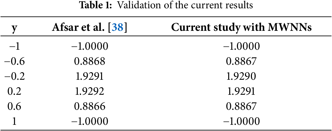
To validate the current results and to ensure the accuracy of MWNNs, Table 1 is prepared by neglecting the effects of electroosmosis Uhs and the Sisko fluid factor m∗. From the table, we can verify that the current results are showing a great matching with the results of Afsar et al. [38] which clarify that MWNNs produced accurate results.

6  Conclusions

The objective of this study was to design a framework for simulating the effects of thermally radiative Sisko nanofluid and viscous dissipation on peristaltic waves in an asymmetric channel, considering double diffusion convection, electroosmosis, and induced magnetohydrodynamics. The governing equations for a Sisko nanofluid incorporating simultaneous diffusion, convection, and nanoparticle dynamics were formulated and simplified under the assumption of long wavelength. This yielded a set of partial differential equations that are nonlinear. To acquire numerical solutions, an integrated unsupervised Morlet wavelet neural network approach was employed. Convergence was evaluated using statistical metrics such as the mean squared error and the Theil inequality coefficient. Across fifty independent runs, the convergence values ranged between 10−5 to 10−7 for the Theil inequality coefficient and 10−7 to 10−10 for the mean squared error, demonstrating that the proposed method is both reliable and rapidly convergent. The graphical results highlight the influence of numerous physical parameters on velocity, temperature, concentration, and pressure fields, thereby providing deeper insight into the transport mechanisms of Sisko nanofluid flows. Key findings from that research include the following facts:

⮚   The velocity displays an upsurge as Helmholtz–Smoluchowski velocity escalations, whereas for the nanoparticle Grashof number, the velocity undergoes an initial slowdown, then a speed up. These results demonstrate that in the presence of electroosmotic factors, velocity significantly upgraded as conpared with the non-electroosmotic scenario [43].

⮚   The nanoparticle fraction increases in the presence of strong radiation effects.

⮚   The magnetic force function (ξ) is negatively impacted by the electric field, while it is positively influenced by the magnetic Reynolds number.

⮚   The pressure gradient profile rises with the Sisko fluid parameter, then declines with the Hartmann number, the thermal Grashof number, and the Joule heating parameter.

⮚   The pressure rise per wavelength indicates a substantial increase with the Brinkman number in the augmented pumping region.

⮚   The streamline graphs exhibit an upward trend in bolus size with progressive increments in the Helmholtz–Smoluchowski velocity.

⮚   In the future, we aim to extend this framework by employing quantum-based unsupervised machine learning integrated with heuristic algorithms, which have the potential to tackle complex nonlinear fluid flow problems more efficiently and accurately than existing methods.

It should be noted that the present study is restricted to a two-dimensional channel geometry under limitations of lubrication and long wavelength approximations. Extending the model to three-dimensional domains and validating it with experimental data remain important directions for future research.

Acknowledgement: Not applicable.

Funding Statement: The author received no specific funding for this study.

Author Contributions: The authors confirm contribution to the paper as follows: Conceptualization and supervision, Arshad Riaz; formal analysis and writing—original draft preparation, Misbah Ilyas; methodology, Muhammad Naeem Aslam; investigation, Safia Akram; visualization and resources, Sami Ullah Khan; validation and writing—review and editing, Ghaliah Alhamzi. All authors reviewed the results and approved the final version of the manuscript.

Availability of Data and Materials: Not applicable.

Ethics Approval: Not applicable.

Conflicts of Interest: The authors declare no conflicts of interest to report regarding the present study.

Nomenclature

Appendix A

E1=(∂2θ∂y2+NTCPr∂2γ∂y2+NbPr(∂θ∂y∂Ω∂y)+NtPr(∂θ∂y)2+RdPr∂2θ∂y2+Br(∂2ψ∂y2)(∂2ψ∂y2+m∗(∂2ψ∂y2)b)+Prβ)2

E2=∑i=1t(∂2γ∂y2+NCT∂2θ∂y2)2

E3=∑i=1t(∂2∂y2((1+m∗((∂2ψ∂y2)2)b−12)∂2ψ∂y2)−M2∂2ψ∂y2+Grt∂θ∂y+Grc∂γ∂y−GrF∂Ω∂y+Uhs∂3ω∂y3)2

E4=∑i=1t(((uf^(0)+1)2+(∂2uf^(0)∂y2)2+(θ^(0))2+(θ^(h)−1)2+(ϕ^(0))2+(ϕ^(h)−1)2))

E=E1+E2+E3+E4

References

1. Latham TW. Fluid motions in a peristaltic pump [dissertation]. Minnesota, MN, USA: Massachusetts Institute of Technology; 1966. [Google Scholar]

2. Barton C, Raynor S. Peristaltic flow in tubes. Bull Math Biophys. 1968 Dec;30(4):663–80. doi:10.1007/BF02476682. [Google Scholar] [PubMed] [CrossRef]

3. Riaz A, Bhatti MM, Ellahi R, Zeeshan A, M. Sait S. Mathematical analysis on an asymmetrical wavy motion of blood under the influence entropy generation with convective boundary conditions. Symmetry. 2020 Jan 6;12(1):102. doi:10.3390/sym12010102. [Google Scholar] [CrossRef]

4. Srinivas S, Anasuya JB, Merugu V. Interaction of pulsatile and peristaltic flow of a particle-fluid suspension with thermal effects. Int Commun Heat Mass Transf. 2025 Apr 1;163:108728. doi:10.1016/j.icheatmasstransfer.2025.108728. [Google Scholar] [CrossRef]

5. Jagadesh V, Sreenadh S, Ajithkumar M, Lakshminarayana P, Sucharitha G. Numerical exploration of the peristaltic flow of MHD Jeffrey nanofluid through a non-uniform porous channel with Arrhenius activation energy. Numer Heat Transf Part A: Appl. 2025 Aug 18;86(16):5542–56. doi:10.1080/10407782.2024.2332477. [Google Scholar] [CrossRef]

6. Akbar Y, Abbasi FM. Impact of variable viscosity on peristaltic motion with entropy generation. Int Commun Heat Mass Transf. 2020 Nov 1;118:104826. doi:10.1016/j.icheatmasstransfer.2020.104826. [Google Scholar] [CrossRef]

7. Akbar NS, Hayat T, Nadeem S, Obaidat S. Peristaltic flow of a Williamson fluid in an inclined asymmetric channel with partial slip and heat transfer. Int J Heat Mass Transf. 2012 Mar 1;55(7–8):1855–62. doi:10.1016/j.ijheatmasstransfer.2011.11.038. [Google Scholar] [CrossRef]

8. Akram S, Mekheimer KS, Nadeem S. Influence of lateral walls on peristaltic flow of a couple stress fluid in a non-uniform rectangular duct. Appl Math Inform Sci. 2014 May 1;8(3):1127. doi:10.12785/amis/080323. [Google Scholar] [CrossRef]

9. Nadeem S, Akram S. Peristaltic flow of a Williamson fluid in an asymmetric channel. Commun Nonlinear Sci Numer Simul. 2010 Jul 1;15(7):1705–16. doi:10.1016/j.cnsns.2009.07.026. [Google Scholar] [CrossRef]

10. Akhtar S, Almutairi S, Nadeem S. Impact of heat and mass transfer on the Peristaltic flow of non-Newtonian Casson fluid inside an elliptic conduit: exact solutions through novel technique. Chin J Phys. 2022 Aug 1;78:194–206. doi:10.1016/j.cjph.2022.06.013. [Google Scholar] [CrossRef]

11. Khan AA, Zahra B, Ellahi R, Sait SM. Analytical solutions of peristalsis flow of non-Newtonian Williamson fluid in a curved micro-channel under the effects of electro-osmotic and entropy generation. Symmetry. 2023 Apr 9;15(4):889. doi:10.3390/sym15040889. [Google Scholar] [CrossRef]

12. Hussain A, Malik MY, Salahuddin T, Bilal S, Awais M. Combined effects of viscous dissipation and Joule heating on MHD Sisko nanofluid over a stretching cylinder. J Mol Liq. 2017 Apr 1;231:341–52. doi:10.1016/j.molliq.2017.02.030. [Google Scholar] [CrossRef]

13. Choi SU, Eastman JA. Enhancing thermal conductivity of fluids with nanoparticles. Argonne, IL, USA: Argonne National Lab (ANL); 1995. [Google Scholar]

14. Akbar NS. Peristaltic Sisko nano fluid in an asymmetric channel. Appl Nanosci. 2014 Aug;4(6):663–73. doi:10.1007/s13204-013-0205-1. [Google Scholar] [CrossRef]

15. Trisaksri V, Wongwises S. Critical review of heat transfer characteristics of nanofluids. Renew Sustain Energ Rev. 2007 Apr 1;11(3):512–23. doi:10.1016/j.rser.2005.01.010. [Google Scholar] [CrossRef]

16. Ullah H, Abas SA, Fiza M, Jan AU, Akgul A, Abd El-Rahman M, et al. Thermal radiation effects of ternary hybrid nanofluid flow in the activation energy: numerical computational approach. Results Eng. 2025 Mar 1;25:104062. doi:10.1016/j.rineng.2025.104062. [Google Scholar] [CrossRef]

17. Akram S, Afzal Q, Aly EH. Half-breed effects of thermal and concentration convection of peristaltic pseudoplastic nanofluid in a tapered channel with induced magnetic field. Case Stud Therm Eng. 2020 Dec 1;22:100775. doi:10.1016/j.csite.2020.100775. [Google Scholar] [CrossRef]

18. Akram S, Athar M, Saeed K. Hybrid impact of thermal and concentration convection on peristaltic pumping of Prandtl nanofluids in non-uniform inclined channel and magnetic field. Case Stud Therm Eng. 2021 Jun 1;25:100965. doi:10.1016/j.csite.2021.100965. [Google Scholar] [CrossRef]

19. Khan Y, Akram S, Athar M, Saeed K, Razia A, Alameer A. Mechanism of thermally radiative prandtl nanofluids and double-diffusive convection in tapered channel on peristaltic flow with viscous dissipation and induced magnetic field. Comput Model Eng Sci. 2024;138(2):1501–20. doi:10.32604/cmes.2023.029878. [Google Scholar] [CrossRef]

20. Khazayinejad M, Hafezi M, Dabir B. Peristaltic transport of biological graphene-blood nanofluid considering inclined magnetic field and thermal radiation in a porous media. Powder Technol. 2021 May 1;384:452–65. doi:10.1016/j.powtec.2021.02.036. [Google Scholar] [CrossRef]

21. Nisar Z, Hayat T, Alsaedi A, Momani S. Mathematical modelling for peristaltic flow of fourth-grade nanoliquid with entropy generation. ZAMM-J Appl Math Mech/Zeitschrift Für Angewandte Mathematik Und Mechanik. 2024 Jan;104(1):99. doi:10.1002/zamm.202300034. [Google Scholar] [CrossRef]

22. Alghamdi M, Fatima B, Hussain Z, Nisar Z, Alghamdi HA. Peristaltic pumping of hybrid nanofluids through an inclined asymmetric channel: a biomedical application. Mater Today Commun. 2023 Jun 1;35:105684. doi:10.1016/j.mtcomm.2023.105684. [Google Scholar] [CrossRef]

23. Ali A, Ali Y, Khan Marwat DN, Awais M, Shah Z. Peristaltic flow of nanofluid in a deformable channel with double diffusion. SN Appl Sci. 2020 Jan;2(1):1232. doi:10.1007/s42452-019-1867-4. [Google Scholar] [CrossRef]

24. Alolaiyan H, Riaz A, Razaq A, Saleem N, Zeeshan A, Bhatti MM. Effects of double diffusion convection on third grade nanofluid through a curved compliant peristaltic channel. Coatings. 2020 Feb 8;10(2):154. doi:10.3390/coatings10020154. [Google Scholar] [CrossRef]

25. Shivappa Kotnurkar A, Giddaiah S. Double diffusion on peristaltic flow of nanofluid under the influences of magnetic field, porous medium, and thermal radiation. Eng Reports. 2020 Feb;2(2):6958. doi:10.1002/eng2.12111. [Google Scholar] [CrossRef]

26. Uddin I, Ullah I, Raja MA, Shoaib M, Islam S, Zobaer MS, et al. The intelligent networks for double-diffusion and MHD analysis of thin film flow over a stretched surface. Sci Rep. 2021;11(1):19239. doi:10.1038/s41598-021-97458-2. [Google Scholar] [PubMed] [CrossRef]

27. Akbar NS, Zamir T, Alzubaidi A, Saleem S. Thermally simulated double diffusion flow for Prandtl nanofluid through Levenberg-Marquardt scheme with artificial neural networks with chemical reaction and heat transfer. J Therm Anal Calorim. 2025 Jan;150(1):627–47. doi:10.1007/s10973-024-13831-z. [Google Scholar] [CrossRef]

28. Ajithkumar M, Lakshminarayana P. Chemically reactive MHD peristaltic flow of Jeffrey nanofluid via a vertical porous conduit with complaint walls under the effects of bioconvection and double diffusion. Int J Mod Phys B. 2024 Jun 30;38(16):2450203. doi:10.1142/S0217979224502035. [Google Scholar] [CrossRef]

29. Sher Akbar N, Zamir T, Bilal S, Muhammad T. Computational study with neural networks to double diffusion in Prandtl thermal nanofluid flow adjacent to a stretching surface design with numerical treatment. Proc Instit Mech Eng Part N J Nanomater Nanoeng Nanosyst. 2024:23977914241289978. doi:10.1177/23977914241289978. [Google Scholar] [CrossRef]

30. Hussain A, Farooq N, Saddiqa A. Exploration of double diffusive convection phenomena of viscous nanofluid with consideration of solar radiative flux and MHD impact through the peristaltic channel. Numer Heat Transf Part B Fundam. 2025 Mar 4;86(3):373–401. doi:10.1080/10407790.2023.2283557. [Google Scholar] [CrossRef]

31. Chakraborty S. Augmentation of peristaltic microflows through electro-osmotic mechanisms. J Phys D Appl Phys. 2006 Dec 1;39(24):5356. doi:10.1088/0022-3727/39/24/037. [Google Scholar] [CrossRef]

32. Tripathi D, Bhushan S, Bég OA. Transverse magnetic field driven modification in unsteady peristaltic transport with electrical double layer effects. Coll Surf A Physicochem Eng Aspects. 2016 Oct 5;506:32–9. doi:10.1016/j.colsurfa.2016.06.004. [Google Scholar] [CrossRef]

33. Misra JC, Chandra S, Shit GC, Kundu PK. Electroosmotic oscillatory flow of micropolar fluid in microchannels: application to dynamics of blood flow in microfluidic devices. Appl Math Mech. 2014 Jun;35(6):749–66. doi:10.1007/s10483-014-1827-6. [Google Scholar] [CrossRef]

34. Goswami P, Chakraborty J, Bandopadhyay A, Chakraborty S. Electrokinetically modulated peristaltic transport of power-law fluids. Microvasc Res. 2016 Jan 1;103:41–54. doi:10.1016/j.mvr.2015.10.004. [Google Scholar] [PubMed] [CrossRef]

35. McKnight TE, Culbertson CT, Jacobson SC, Ramsey JM. Electroosmotically induced hydraulic pumping with integrated electrodes on microfluidic devices. Anal Chem. 2001 Aug 15;73(16):4045–9. doi:10.1021/ac010048a. [Google Scholar] [PubMed] [CrossRef]

36. Reddy MG, Reddy KV, Souayeh B, Fayaz H. Numerical entropy analysis of MHD electro-osmotic flow of peristaltic movement in a nanofluid. Heliyon. 2024 March 15;35(5):e27185. doi:10.1016/j.heliyon.2024.e27185. [Google Scholar] [PubMed] [CrossRef]

37. Afonso AM, Alves MA, Pinho FT. Analytical solution of two-fluid electro-osmotic flows of viscoelastic fluids. J Colloid Interface Sci. 2013 Apr 1;395(1):277–86. doi:10.1016/j.jcis.2012.12.013. [Google Scholar] [PubMed] [CrossRef]

38. Afsar H, Peiwei G, Alshamrani A, Alam MM, Hendy AS, Zaky MA. Electroosmotically induced peristaltic flow of a hybrid nanofluid in asymmetric channel: revolutionizing nanofluid engineering. Case Stud Therm Eng. 2023 Nov 19;52(2023):103779. doi:10.1016/j.csite.2023.103779. [Google Scholar] [CrossRef]

39. Kumar A, Tripathi D, Tiwari AK, Seshaiyer P. Magnetic field modulation of electroosmotic-peristaltic flow in tumor microenvironment. Phys Fluids. 2025 Apr 1;37(4):3121. doi:10.1063/5.0264693. [Google Scholar] [CrossRef]

40. Das S, Chakraborty S. Analytical solutions for velocity, temperature and concentration distribution in electroosmotic microchannel flows of a non-Newtonian bio-fluid. Anal Chim Acta. 2006 Feb 10;559(1):15–24. doi:10.1016/j.aca.2005.11.046. [Google Scholar] [CrossRef]

41. Bilal S, Akram S, Saeed K, Athar M, Riaz A, Razia A. A computational simulation for peristaltic flow of thermally radiative sisko nanofluid with viscous dissipation, double diffusion convection and induced magnetic field. Numer Heat Transf Part A Appl. 2025 Sep 2;86(17):5927–48. doi:10.1080/10407782.2024.2335557. [Google Scholar] [CrossRef]

42. Mekheimer KS. Effect of the induced magnetic field on peristaltic flow of a couple stress fluid. Phys Lett A. 2008 Jun 2;372(23):4271–8. doi:10.1016/j.physleta.2008.03.059. [Google Scholar] [CrossRef]

43. Bég OA, Tripathi D. Mathematica simulation of peristaltic pumping with double-diffusive convection in nanofluids: a bio-nano-engineering model. Proc Instit Mech Eng Part N J Nanoeng Nanosyst. 2011 Sep;225(3):99–114. doi:10.1177/1740349912437087. [Google Scholar] [CrossRef]

44. Turkyilmazoglu M. Corrections to long wavelength approximation of peristalsis viscous fluid flow within a wavy channel. Chin J Phys. 2024 Jun 1;89:340–54. doi:10.1016/j.cjph.2024.03.030. [Google Scholar] [CrossRef]

45. Eberhart R, Kennedy J. A new optimizer using particle swarm theory. In: MHS’95. Proceedings of the Sixth International Symposium on Micro Machine and Human Science; 1995 Oct 4; Nagoya, Japan. Piscataway, NJ, USA:IEEE. 1995; p. 39–43. doi:10.1109/MHS.1995.494215. [Google Scholar] [CrossRef]

46. Panda S, Padhy NP. Comparison of particle swarm optimization and genetic algorithm for FACTS-based controller design. Appl Soft Comput. 2008 Sep 1;8(4):1418–27. doi:10.1016/j.asoc.2007.10.009. [Google Scholar] [CrossRef]

47. Okwu MO, Tartibu LK. Particle swarm optimisation. In: Metaheuristic optimization: nature-inspired algorithms swarm and computational intelligence, theory and applications. Cham, Switzerland: Springer International Publishing; 2020. p. 5–13. doi:10.1007/978-3-030-61111-8_2. [Google Scholar] [CrossRef]

48. Yu Y, Yin S. A comparison between generic algorithm and particle swarm optimization. In: Proceedings of the 1st International Symposium on Artificial Intelligence in Medical Sciences; 2020 Sep 11. p. 137–9. doi:10.1145/3429889.3430294. [Google Scholar] [CrossRef]

49. Stacey A, Jancic M, Grundy I. Particle swarm optimization with mutation. In: The 2003 Congress on Evolutionary Computation, 2003. CEC’03; 2003 Dec 8; Canberra, Australia. Piscataway, NJ, USA: IEEE. 2003; Vol. 2. p. 1425–30. doi:10.1109/CEC.2003.1299838. [Google Scholar] [CrossRef]

50. Toushmalani R. Gravity inversion of a fault by particle swarm optimization (PSO). SpringerPlus. 2013 Jul 15;2(1):315. doi:10.1186/2193-1801-2-315. [Google Scholar] [PubMed] [CrossRef]

51. Bassi SJ, Mishra MK, Omizegba EE. Automatic tuning of proportional-integral-derivative (PID) controller using particle swarm optimization (PSO) algorithm. Int J Artif Intell Appl. 2011 Oct 1;2(4):25. doi:10.5121/ijaia.2011.2403. [Google Scholar] [CrossRef]

52. Esmin AA, Coelho RA, Matwin S. A review on particle swarm optimization algorithm and its variants to clustering high-dimensional data. Artif Intell Rev. 2015 Jun;44(1):23–45. doi:10.1007/s10462-013-9400-4. [Google Scholar] [CrossRef]

53. Turkyilmazoglu M, Alotaibi A. On the viscous flow through a porous-walled pipe: asymptotic MHD effects. Microfluid Nanofluidics. 2025 Jun;29(6):1. doi:10.1007/s10404-025-02808-5. [Google Scholar] [CrossRef]