
 Submit a Paper
 Propose a Special lssue
 Open Access
ARTICLE
Optimization and Sensitivity Analysis of Non-Isothermal Carreau Fluid Flow in Roll Coating Systems with Fixed Boundary Constraints: A Comparative Investigation
1 College of Mathematics and System Sciences, Xinjiang University, Urumqi, 830046, China
2 Department of Mathematics, COMSATS University Islamabad, Abbottabad, 22060, Pakistan
* Corresponding Authors: Fateh Ali. Email: ; Xinlong Feng. Email:
Computer Modeling in Engineering & Sciences 2025, 145(3), 3511-3561. https://doi.org/10.32604/cmes.2025.073678
Received 23 September 2025; Accepted 18 November 2025; Issue published 23 December 2025
 View Full Text
 Download PDF
Abstract
Roll coating is a vital industrial process used in printing, packaging, and polymer film production, where maintaining a uniform coating is critical for product quality and efficiency. This work models non-isothermal Carreau fluid flow between a rotating roll and a stationary wall under fixed boundary constraints to evaluate how non-Newtonian and thermal effects influence coating performance. The governing equations are transformed into non-dimensional form and simplified using lubrication approximation theory. Approximate analytical solutions are obtained via the perturbation technique, while numerical results are computed using both the finite difference method and the BVP-Midrich technique. Furthermore, Response surface methodology (RSM) is employed for optimization and sensitivity analysis. Analytical and numerical results show strong agreement (<1% deviation). The model predicts coating thicknessKeywords
The Classical Navier-Stokes equations are insufficient to describe the rheological complex fluids, motivating the development of constitutive models for non-Newtonian behavior. Interest in non-Newtonian fluid mechanics has grown because of extensive applications in medical devices, manufacturing, energy, and process engineering [1]. Examples include sludge, polymers, crude oil, cosmetics and soap solutions, petroleum products, drilling fluids, and coatings. The role of non-Newtonian fluids in enhancing coating performance offers significant benefits for achieving a uniform, thin-coated layer on a surface. The constitutive relationship between stress and deformation rate tensor is shown using several rheological models. There are many fluid models available, including those by Jeffrey, Sisko, Casson, differential types, grade n fluids (e.g., Phan Thien and Tanner), Maxwell, elastic-viscous, Oldroyd’s family, and Carreau [2,3]. The non-linear properties of non-Newtonian fluids present difficulties in deriving solutions by analytical and numerical techniques. The complexity of these fluids requires alterations to the governing formulas. The major governing equations are formulated by adjusting the momentum equation to incorporate the stress tensor obtained from the constitutive equation. To transform the set of equations, the lubrication approximation method (LAT) is applied, and specific boundary conditions have been established in alignment with the specified problem. This article covers numerical solutions through the finite difference method (FDM) [4], the Midrich boundary value problem (BVP) method [5], and analytical solutions using the Perturbation method (PM) [6].
The process of applying a consistent layer of liquid to a moving substrate is called roll coating (RC) [7]. This process is extensively employed to apply accurate and uniform coatings on various substrates, including magnetic electronic media, adhesive tapes, foils, plastic films, printed materials, paper, and paperboard. This procedure enhances the functional and aesthetic properties of products, including gloss, printability, and smoothness, while also improving their durability, performance, and resistance to environmental influences. Fig. 1 illustrates a schematic of the roll-coating setup analyzed in this study. Where a rotating roll moves upward, entraining a non-Newtonian Carreau fluid into the narrow nip region created between the roll and a stationary constrained wall. The confined gap induces significant shear, pressure, and heat-transfer effects that shape the film development. As the roll extends beyond the wall, a uniform coating layer adheres to its surface, influenced by geometric parameters, like roll radius, wall position, and nip gap, governing the velocity, pressure, temperature, and coating uniformity.
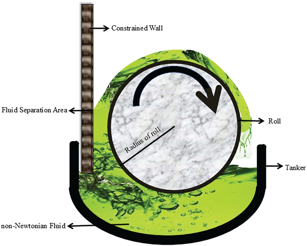
Figure 1: Diagram exhibiting the RC configuration specific to the current problem [8]
Significant studies integrating analytical, experimental, and computational methodologies regarding the roll-coating (RC) process have been reported in Greener and Middleman [9] investigated the RC process of a viscoelastic fluid utilizing the conventional LAT and derived the solution via the perturbation approach. They observed a decline in the pressure with a slight increase in coating thickness. Coyle [7] previously conducted a thorough examination of the fluid dynamics of RC, focusing on steady flows, rheology, and stability, and clarifying the critical flow characteristics, stability factors, and rheological influences involved in these processes. Hinter and White [10] examined the water flow occurring between two rolls in their research findings. The lubricating principle was employed to confirm that the results aligned with the experimental data.
Previous investigations have significantly contributed to the understanding of roll-coating flows. Greener and Middleman [11] established analytical and experimental frameworks linking pressure distribution with coating thickness. However, their work omitted to take surface tension, free surfaces, and contact line behaviour into consideration. Owens et al. [12] investigated misting in RC and determined that it’s non-linearly dependent on time for relaxation as a result of filaments and bead breakdown. Additionally, Lécuyer et al. [13] incorporated roll deformation and free-surface dynamics, demonstrating how roll compliance modifies nip hydrodynamics. Ascanio et al. [14] developed validated computational strategies for high-speed and discrete gravure coating of complex fluids. Echendu [15] implemented analytic and computational methodologies to examine the flow attributes of coatings for a variety of fluid types, including Newtonian and non-Newtonian fluids [16]. These summaries of earlier achievements clarify prior progress and highlight the need for the present study, which integrates non-isothermal Carreau fluid behavior with fixed boundary constraints and optimization analysis.
The study of non-Newtonian fluids has become increasingly significant due to their diverse applications across engineering, industrial processes, and commercial manufacturing [17–20]. Early numerical analyses by, to explore the importance of fluid flow characteristics in the reverse roll coating process (RRCP), Jang and Chen [21] conducted this research by considering the volume of fluid-free surface (VOFFS) and finite-volume (FVM) methodologies. Additionally, Shahzad et al. [22] examined the behavior of a non-isothermal couple stress fluid within an RRC configuration, taking into account the slip conditions present at the surfaces of the rolls. Devisetti and Bousfield [23] investigated the impacts of fluid absorption in forward roll coating (FRC), highlighting the significance of rheological qualities in enhancing industrial efficiency, especially for non-Newtonian lubricants. Bhatti et al. [24] utilized advanced numerical techniques such as the generalized differential quadrature and Newton-Raphson methods to precisely solve non-linear flow and heat transfer equations for magnetized nanofluids. Their approach showed significant stability and precision in predicting velocity, temperature, and concentration distributions over rotating surfaces. Recent research by Farooq et al. [25] has explored nanofluid flows over stretching surfaces under magnetic fields and slip conditions, emphasizing the influence of melting heat, stratification, and nanoparticle additives on heat and mass transfer, particularly through machine learning and neural network-based modeling techniques for enhanced predictive accuracy.
Response surface methodology (RSM) is a statistical technique employed to assess the sensitivity of models to the influencing variables. In recent years, it has been utilized by numerous researchers to address diverse physical problems, with extensive procedures and discussions available in [26,27]. The primary aim of RSM is to optimize responses, making it especially valuable for addressing fluid flow problems where the goal is to enhance desired flow characteristics. More broadly, RSM plays a critical role in enhancing product quality, minimizing costs, and promoting innovation across various industries, including manufacturing, chemical engineering, and coating technologies. The effective implementation of this approach emphasizes the enhancement of achievable outcomes. Consequently, statistical analysis is vital for identifying the relative importance of critical parameters and thereby improving model precision. Furthermore, the strategic application of optimization algorithms to enhance goal functions constitutes a key component of modern decision-making processes.
1.1 Research Gap and Objectives
An extensive examination of the literature reveals a significant gap: Although RC processes with various non-Newtonian fluids have been thoroughly studied [8,28–30], the particular scenario of a non-isothermal Carreau fluid under fixed constraining boundary conditions remains unexplored. The primary objective of our study is to examine how a non-isothermal CRF impacts the heat transfer and flow in the RC process. This configuration is highly relevant for industrial applications, including a stationary bar or wall to regulate control coating thickness. The lack of studies on this particular combination limits the optimization and understanding of such processes. Consequently, the primary objective of this work is to address this gap by rigorously examining the influence of a non-isothermal Carreau fluid on heat transfer and flow dynamics within an RC process featuring a fixed constrained wall. Accordingly, this study fills the identified gap by inquiring:
• How effectively does the non-isothermal Carreau fluid model represent the flow characteristics and coating results with fixed boundary conditions?
• How does the model predict the velocity and temperature distributions under non-isothermal conditions?
• How are the pressure distribution and pressure gradient developed within the coating film, and what do they offer about the flow structure and film formation?
• To what degree can perturbation and numerical methods function as a dependable prediction framework for optimizing roll-coating?
• In what way does the model quantify engineering factors, including coating thickness, power input, and Nusselt number, and evaluate their dependence on the perturbative and gravity parameter for industrial coating applications?
• Why and how do fixed walls alter flow resistance, and what consequences does this have for machine wear and product quality?
The primary aims of our study are:
• Develop analytical (via perturbation approach) and numerical (using BVP Midrich and Finite Difference methods) solutions for the flow and temperature profiles for non-isothermal Carreau fluid.
• Assess the impacts of key physical parameters on critical engineering quantities, including pressure gradient, coating thickness, separation force, and power input.
• Conduct optimization and sensitivity analysis with RSM to determine the optimal process parameters.
• The findings provide new physical insights into how Weissenberg and gravity parameters affect flow behavior, energy consumption, and coating performance, establishing a prediction framework for industrial applications.
Finally, the validity of our results will be confirmed through comprehensive cross-verification between the analytical and numerical methods, as well as comparison with current literature for limited cases. We anticipate excellent agreement, which will validate the robustness of our integrated methodology.
RC is a crucial process in industries such as packaging, printing, and surface protection, where uniform application of liquid films is essential for product quality and material efficiency. The established model and results are directly applicable to roll-to-roll printing, polymer and packaging film production, textile finishing, pharmaceutical and biomedical coatings, as well as decorative or anti-corrosion surface treatments, where controlling film thickness and minimizing mechanical wear are essential. In practical situations, the procedure becomes more complex when addressing non-Newtonian fluids, whose shear-thinning and viscoelastic characteristics significantly influence coating thickness, heat transfer, and energy requirements. Despite its significance, precise modeling of RC with constrained walls remains challenging due to the non-linear characteristics of governing equations and the existence of constrained boundary conditions. By combining perturbation analysis, numerical verification, and statistical optimization, this work provides a comprehensive framework for investigating RC with non-Newtonian fluids. The findings not only advance theoretical understanding of coating flows under constrained boundary conditions but also offer practical insights for improving coating uniformity, optimizing process efficiency, and minimizing material waste in industrial applications. The novelty of this study lies in formulating a complete non-isothermal Carreau fluid model for roll coating under fixed boundary constraints, an unaddressed configuration in the literature.
2 Geometry and Mathematical Formulation
A schematic of the RC system under investigation is presented in Fig. 1. The setup consists of a rotating roller of radius R positioned against a stationary wall. The roller rotates clock-wise with a constant angular velocity
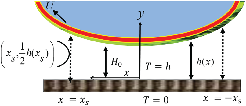
Figure 2: Schematic illustration of the RC process and its variables related to our problem
The coating thickness
Continuity equation [3]:
Momentum equations [31]:
Energy equation [32]:
Extra stress tenor of Carreau Fluid model:
Boundary conditions (BCs) [8]:
•
•
•
•
•
The current study explores the rheological aspects characterized by the viscoelastic CRF model. The equations defining the CRF model are expressed as follows:
we consider the most realistic situations
It is essential to emphasize that within the context of the CRF model, a flow behavior index value (
2.2 Non-Dimensional Form via LAT
On the basis of geometrical data from LAT, our simulations suggest that a significant dynamical event happens in the RC towards the nip. Moreover, LAT is used in those flow geometries in which one dimension is markedly smaller in magnitude relative to others. The surface of the roll is almost parallel to the
The following scales for variation in
Applying Eq. (10) to Eqs. (1)–(5) and yields the following equations in dimensionless form.
2.3 Validity Limits of the Derived Model
“The present formulation is based on the lubrication approximation, valid when the film thickness is much smaller than the roll radius
To obtain practical results for the present analysis, firstly, the PDEs are turned into ODEs by applying certain similarity transformations [8]. The governing equations were first solved analytically by applying the perturbation method, which provided approximate expressions for the flow variables. To validate these results, the problem was reformulated numerically using the finite difference method (FDM) along with Newton’s iteration. The associated non-linear algebraic problem was later solved using Midrich BVP-DSolve in Maple to verify the consistency and stability of the derived solutions. Additionally, RSM was utilized to investigate the impact of key factors and to develop prediction models. A sensitivity study was carried out employing regression-based methodology to identify the most influential variables affecting the system performance. The combined application of perturbation theory, numerical methods, and statistical modeling not only enhances the accuracy of the results but also offers a comprehensive framework for examining the system behavior under different parametric conditions. This hybrid approach ensures both mathematical rigor and practical reliability, hence enhancing the overall credibility of the conclusions. The following flow diagram depicts the full study technique, detailing each stage from model formulation to performance evaluation.
3.1 Asymptotic Solution via Perturbation Method
The perturbation technique is an analytical strategy for solving non-linear ordinary differential equations (ODEs). This approach is frequently employed by engineers to address various real-world difficulties. This is done to guarantee that at least one unknown is shown within a series of smaller factors. This research examines the influence of a very small Weissenberg number
Eqs. (11) and (14) are modified by inserting the relationships in Eq. (17) as given below
By collecting terms of identical orders in
A. Zero-order velocity problem
Eq. (20) is subject to the following BCs:
In accordance with the BCs specified in Eq. (21), the solution to Eq. (20) is as follows:
In the above formulation,
The symbol
Assuming Eq. (23)
By symmetry considerations, the velocity must reduce to zero at the point of separation
by substituting
Substituting
B. First-order velocity problem
For Eq. (28) is subject to the following BCs:
The solution to Eq. (28) under the boundary conditions (29) is as follows:
in Eq. (30),
3.1.1 Temperature Distribution
By simplifying and substituting Eq. (14) into Eq. (17), we get a zeroth- and first-order temperature distribution by equating the corresponding powers of
A. Zero-order temperature problem
The zeroth-order temperature Eq. (32), has the dimensionless BCs:
Taking into consideration the BCs given in Eq. (34), the solution to Eq. (32) is given below:
B. First-order temperature problem
The Eq. (33) is the first-order temperature equation followed with the subsequent dimensionless BCs.
The first-order solution employs a similar methodology to derive the equations for pressure profile, pressure gradient, and detachment locations, quite comparable to the zero-order case. Through the superposition of zero- and first-order solutions, the complete analytical expressions for velocity and temperature are established. The availability of pressure distributions, velocity profiles, and pressure gradients permits expedited determination of critical operating parameters, namely Nusselt number, power input, and the force of roll splitting.
After establishing the pressure gradient, velocity profile, and pressure distributions, engineering parameters such as power input and separation force can be efficiently computed.
4.1 The Force of Roll Separation (Sf)
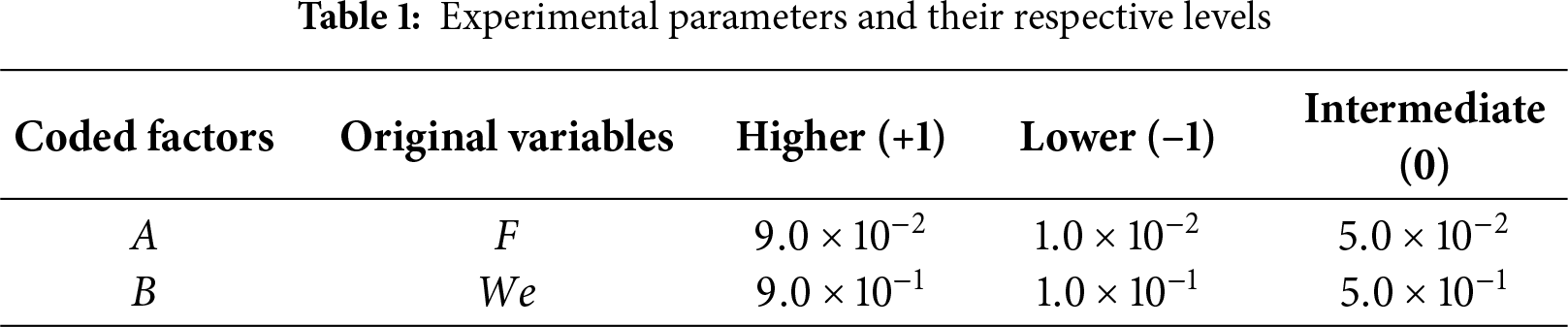
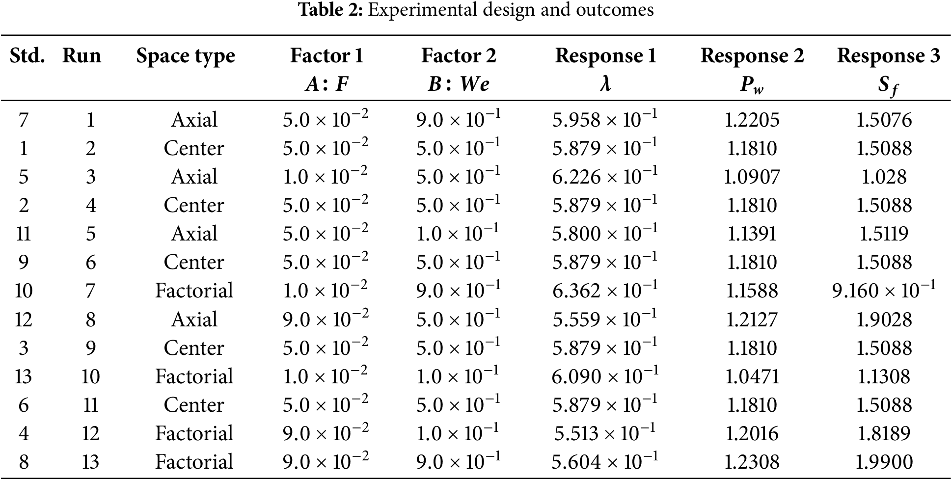
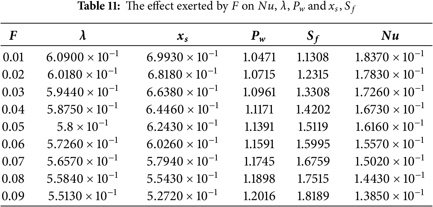
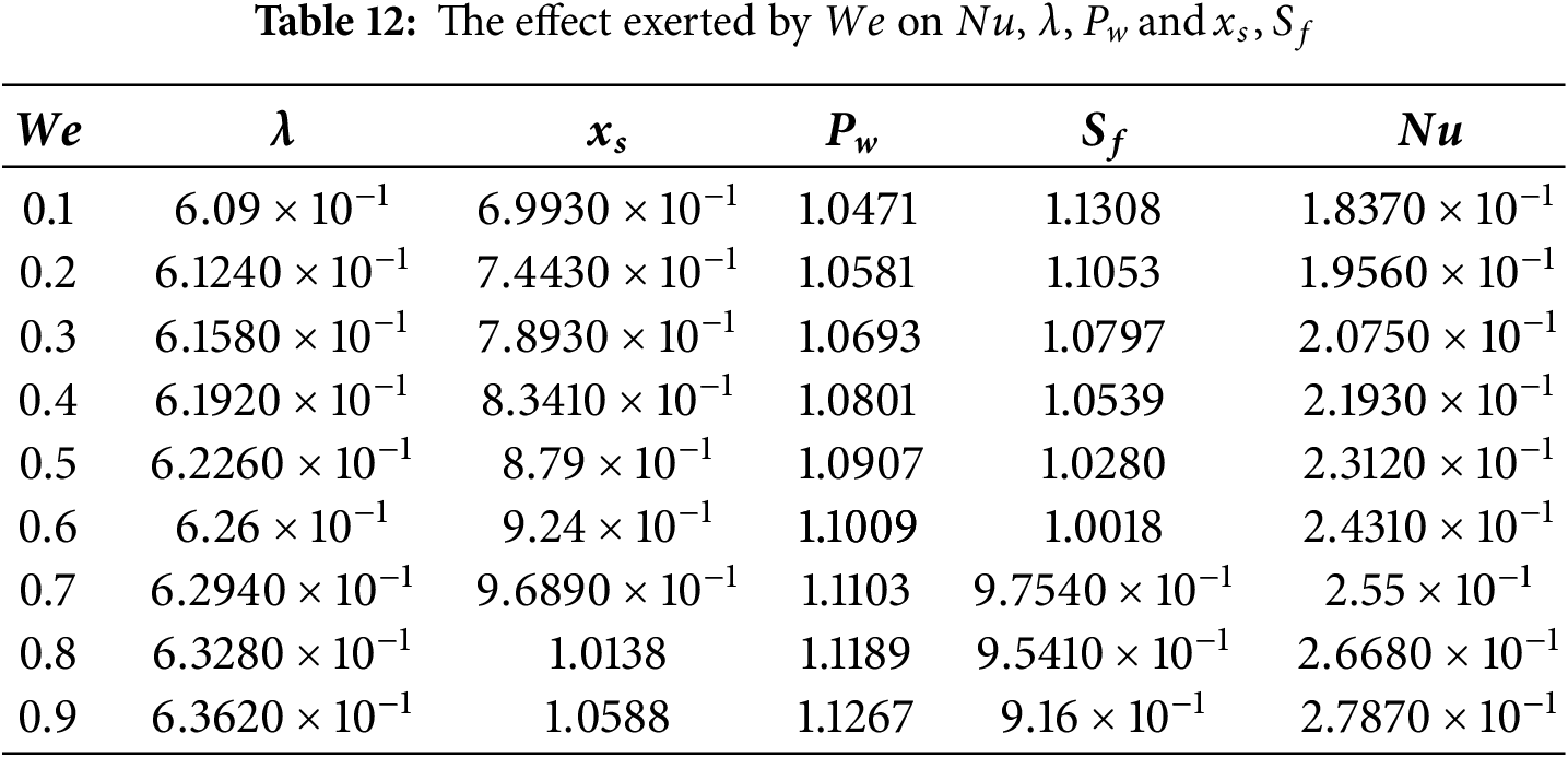
The present investigation requires thirteen runs and twelve degrees of freedom, together with three separate parameter levels, for the use of RSM. The independent variables employed in this study include
Response Surface Method (RSM)
RSM is an optimization method utilized to identify the combination of input parameters that minimizes or maximizes the target function (see Flowchart 1) [29]. The RSM findings provide a practical framework for enhancing roll-coating processes. RSM formulates regression-based models for coating thickness, power input, and separation force to determine the ideal combination of process parameters, including the Weissenberg number and body-force term, that ensures uniform coating while reducing energy consumption. The response surfaces and contour plots illustrate the trade-offs between coating quality and power requirements, allowing process engineers to choose operating conditions that preserve the desired film thickness and stability while minimizing mechanical wear and energy use.
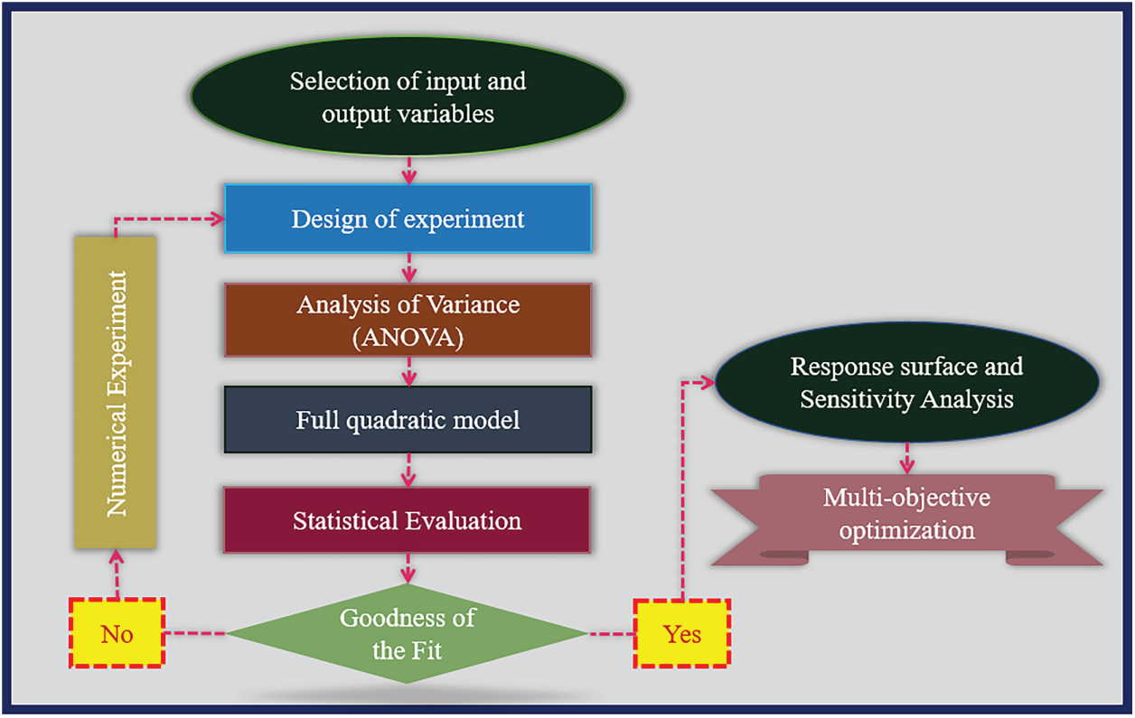
Flowchart 1: Flow chart describing RSM
A central composite design (CCD) that is face-centered is the subject of this study. The CCD approach illustrates the correlation between many predictor factors and one or more responder variables. The inquiry includes two input factors,
where the variables used for regression analysis are denoted as
A. Analysis of variance (ANOVA)
To find out a significant difference in the means of three or more groups, statisticians utilize a process called analysis of variance (ANOVA). We computed and compared
where
where,
The results presented employ adjusted
ANOVA evaluated the model’s adequacy and variable significance via the F-statistic and p-values. The exceptional model F-value (5487.26) and p-values below 0.1000 (Table 3) confirm the model’s high significance and the statistical relevance of its terms. The ANOVA results, confirming the statistical significance of the selected independent variables (
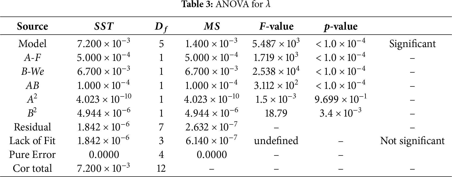
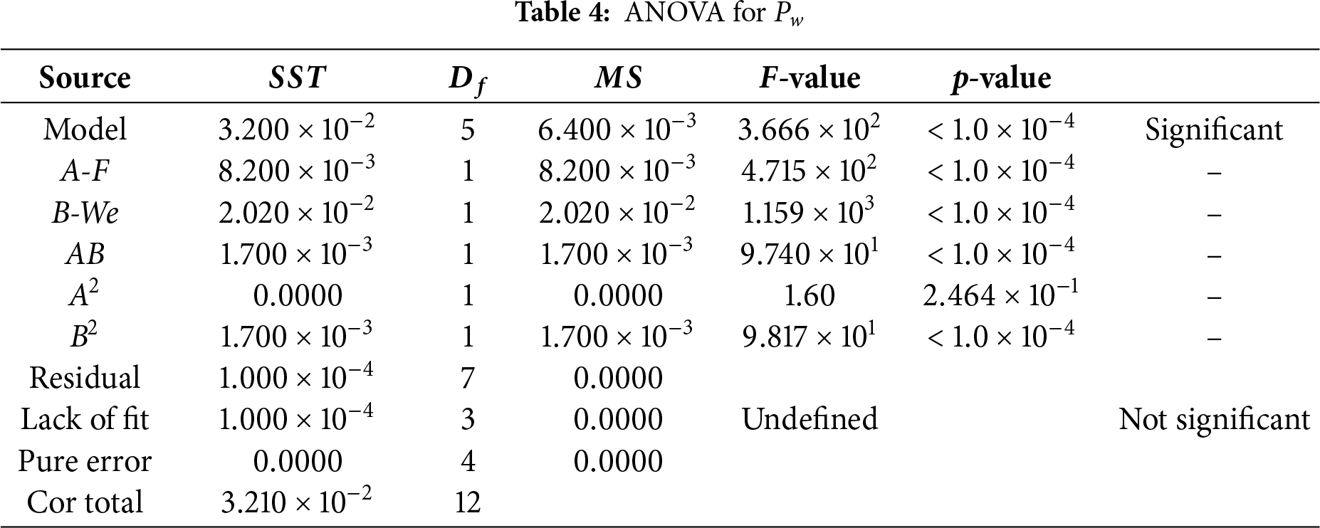
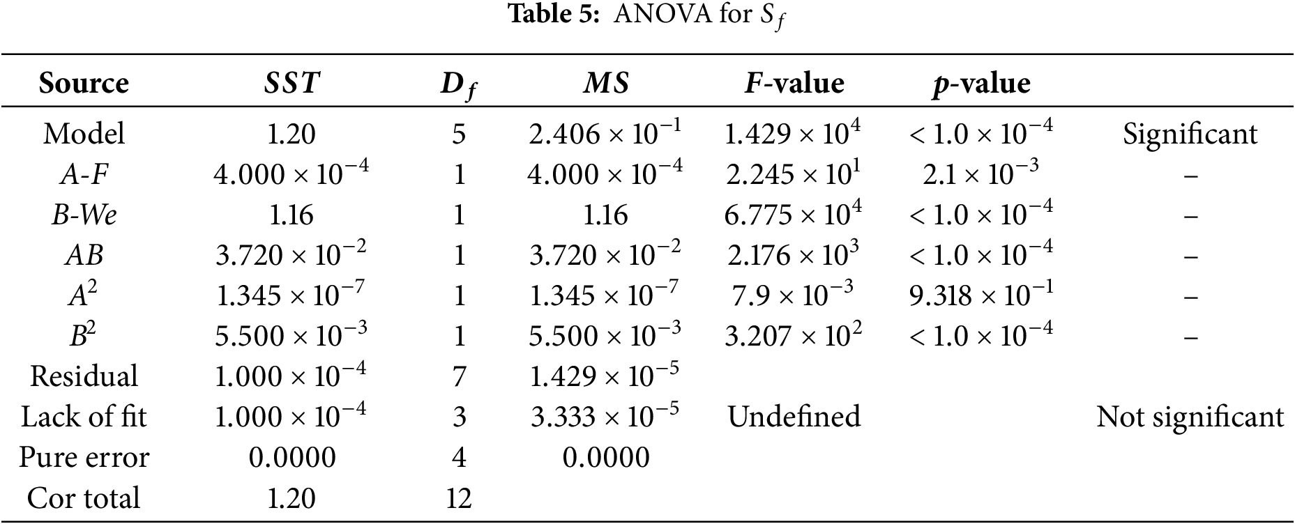
A larger coefficient of determination (
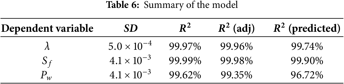
In this study, the value of
B. Regression analysis and model accuracy
Multiple linear regression models that are applicable to the selected range of values are used to estimate
Residual analysis is essential for validating regression model accuracy by diagnosing violations of key statistical assumptions. The Goodness of Fit plot evaluates predictive alignment, while the Normal Probability Plot tests residual normality. Collectively, these graphs identify model inadequacies, refine structure, and ensure robust statistical inferences. Their interpretation is critical for optimizing performance and justifying the real-world applicability of the regression framework.
The residual plots may provide additional evidence of the model’s accuracy. Fig. 3a–c illustrates a major connection between the observed and fitted values as shown in the residuals vs. fitted values graphs. The highest variances are seen to be as little as 0.0005, 0.2, and 0.004, respectively, for
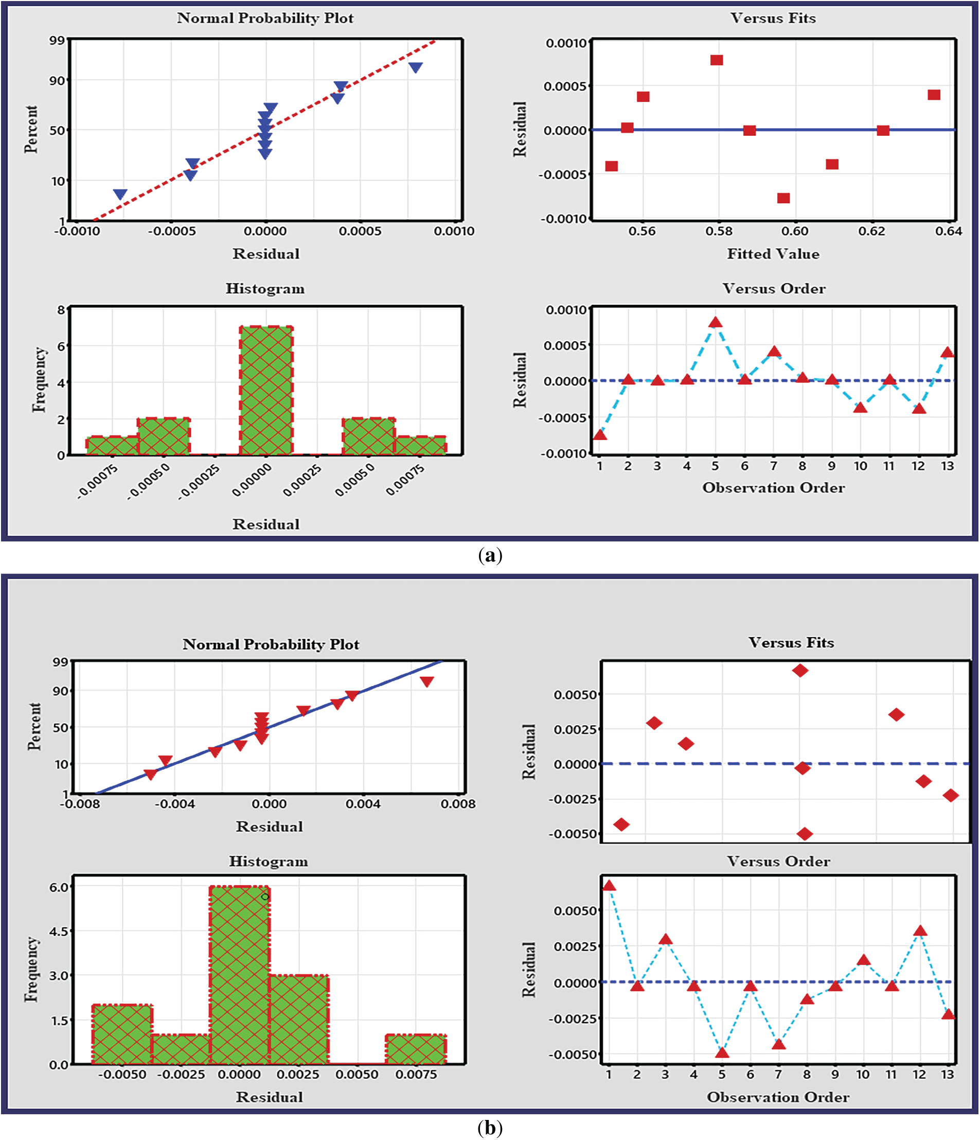
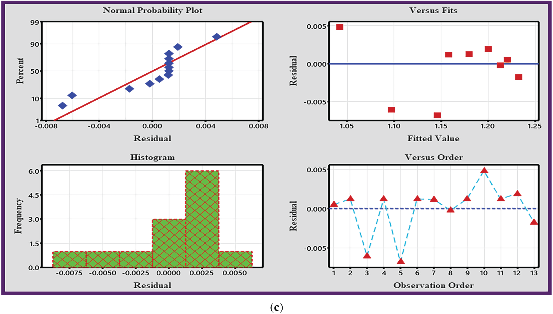
Figure 3: (a). Residual plots for
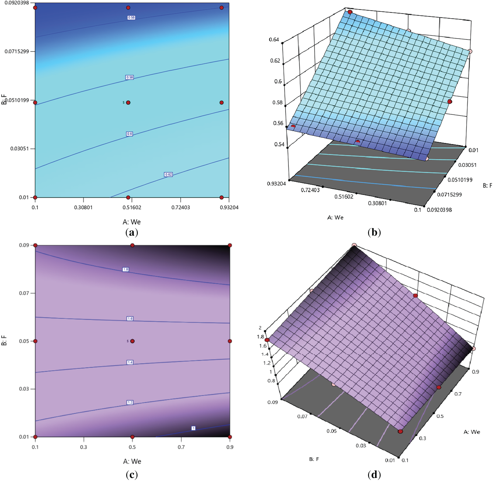
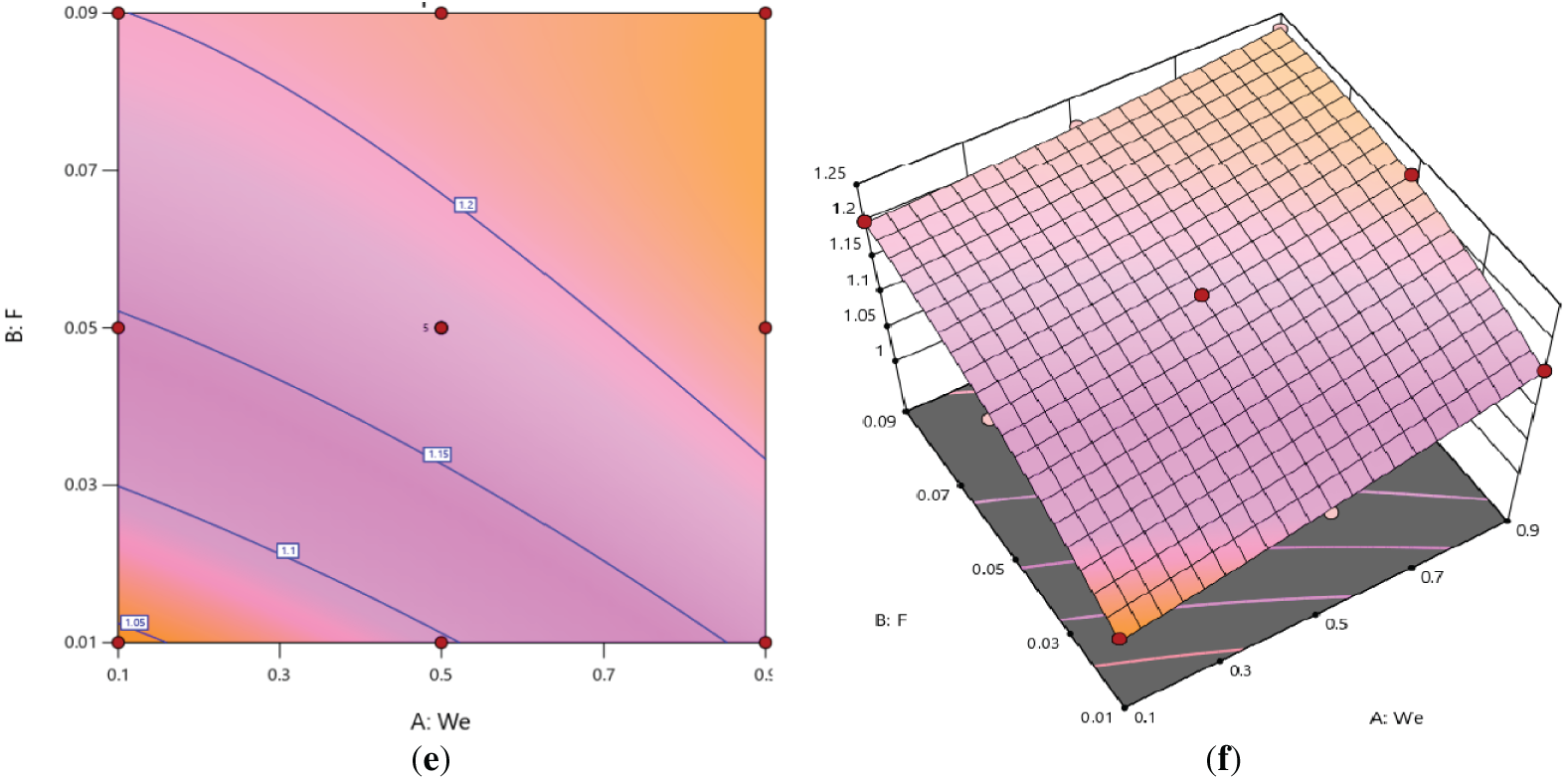
Figure 4: (a–f). Plots in two and three-dimensions showing the impact of surface response on
Contour plots and their corresponding 3-D surface representations illustrate how a function or dataset varies across the domain. In a response surface plot, the
C. Sensitivity analysis
Sensitivity analysis is the initial and important stage in solving optimization problems, as it provides insights into the increasing or decreasing tendencies of the objective function relative to the design parameters. This approach determines essential criteria and prioritizes them according to their significance [29]. The sensitivity of the design objective function to a design variable is defined as the partial derivative of that function with respect to its variables. The estimation of sensitivity is conducted by evaluating the partial derivatives of the response functions (
We compute the partial derivative, or sensitivity function, utilizing the pertinent effective parameters.
where
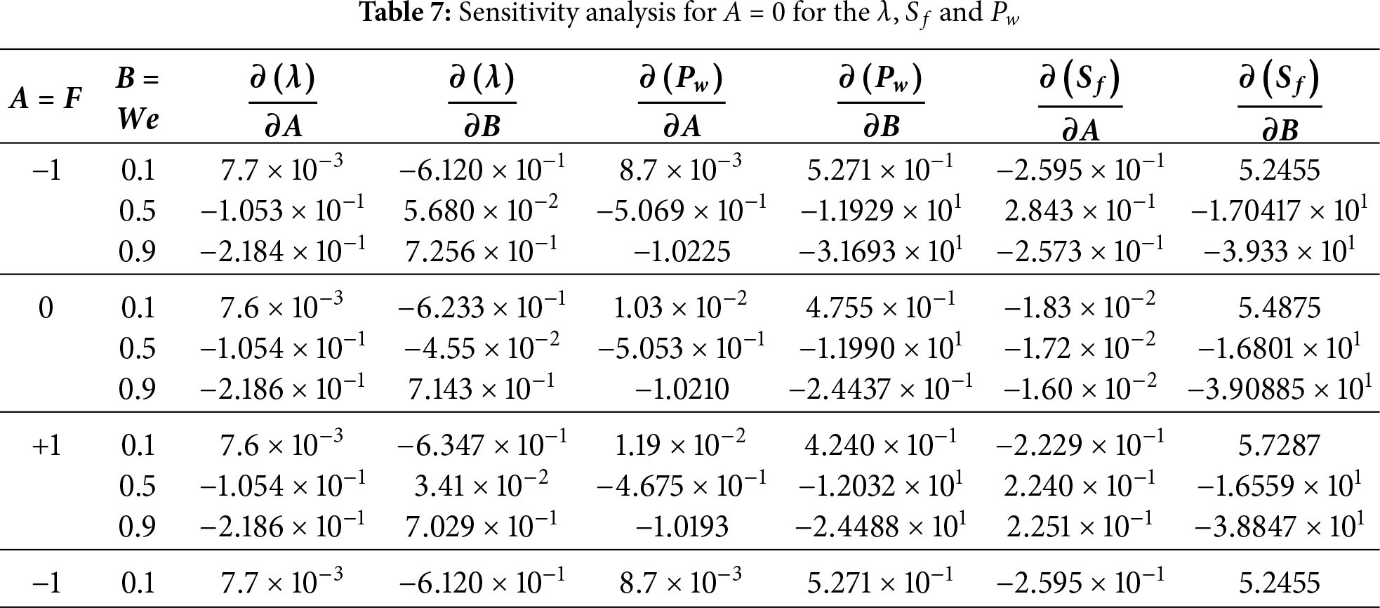
The sensitivity of the key parameters (λ, Pw, Sf) was evaluated at distinct levels of A (−1, 0, 1), as shown in Figs. 5–7. This analysis reveals that a positive sensitivity corresponds to an enhancement of the output function.
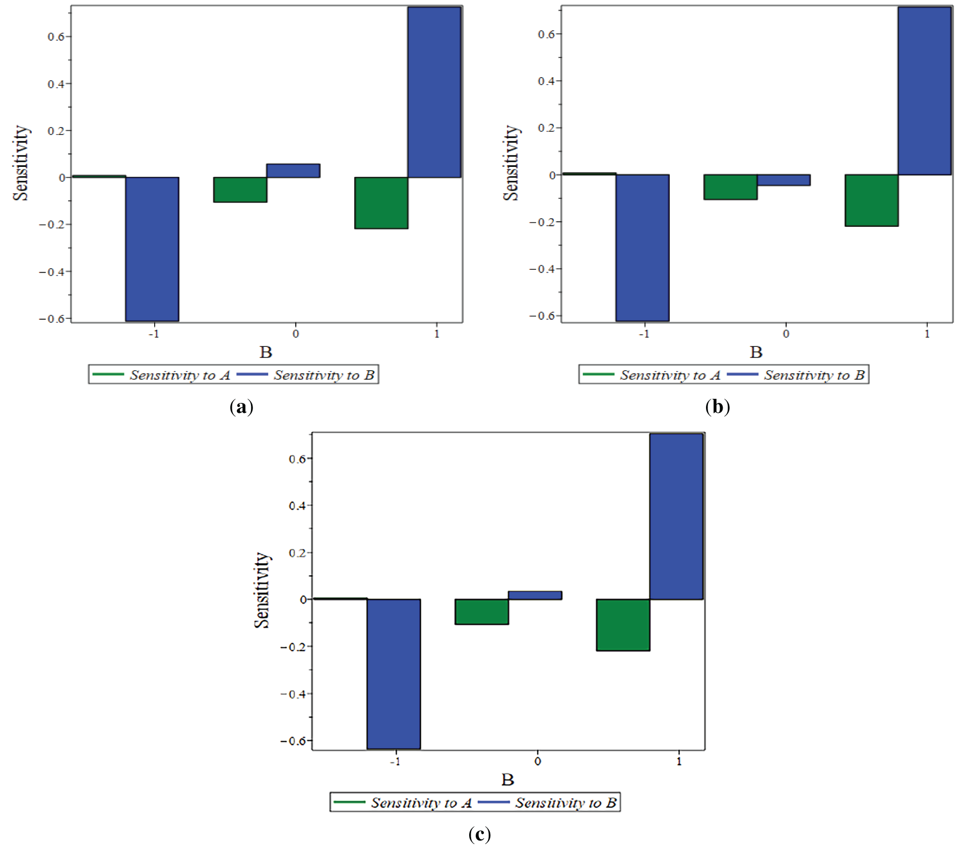
Figure 5:
Figure 6:
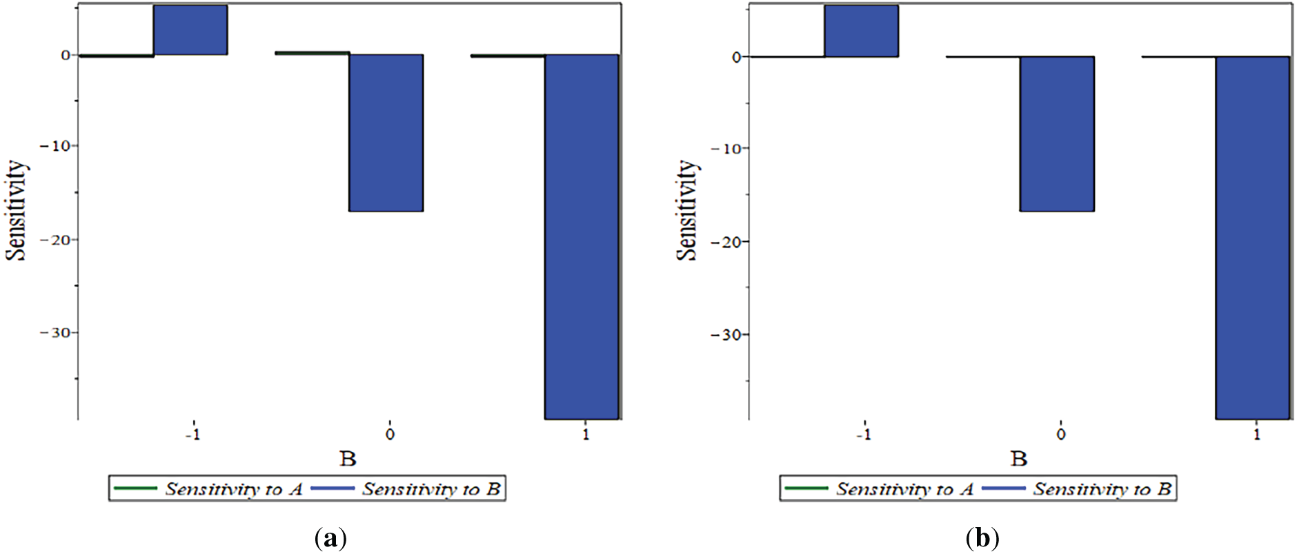
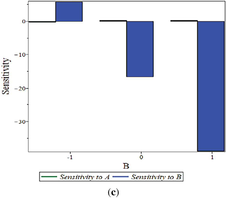
Figure 7:
6 Validation through Numerical Methods
In this section, the results obtained from numerical and analytical approaches are systematically compared. The numerical solutions are computed using the Finite Difference Method (FDM) alongside the BVP-Dsolve solver (Midrich method) implemented in Maple software, enabling an accurate and efficient resolution of the governing equations. The advantages of the BVP Midrich solver are summarized in Flowchart 2. The approximate solution for the temperature and velocity profile is achieved through the PM.
Flowchart 2: Midrich BVP advantages
For a variety of non-linear boundary value problems, there is a numerical approach called the BVP Midrich. A variant of Euler’s midpoint technique is employed in this strategy. Up to a value of 1 × 10⁻⁶, this method demonstrates absolute error convergence. FDM is one of the most effective numerical methods for solving nonlinear coupled ODEs (12) and (15) with suitable boundary conditions. If relevant, it adjusts the differential equations by replacing derivatives with physical domain or time-based interval finite difference approximations. There is a relationship between the number of nodes
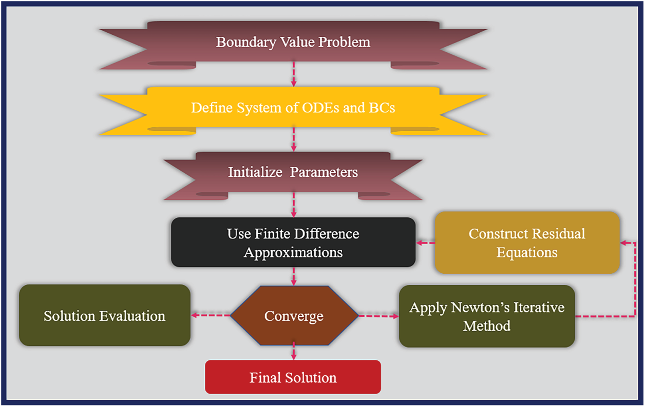
Flowchart 3: Flow chart explaining FDM
The resulting non-linear system was solved iteratively using the Newton iteration approach. The specifics of the linearized system’s construction are left out to keep things brief. We investigate to ensure the analytical and approximate solutions are accurate before giving the results and discussing them. For this purpose, Figs. 8–16 illustrate the velocity and temperature results obtained from both numerical and analytical solutions, considering parameters such as
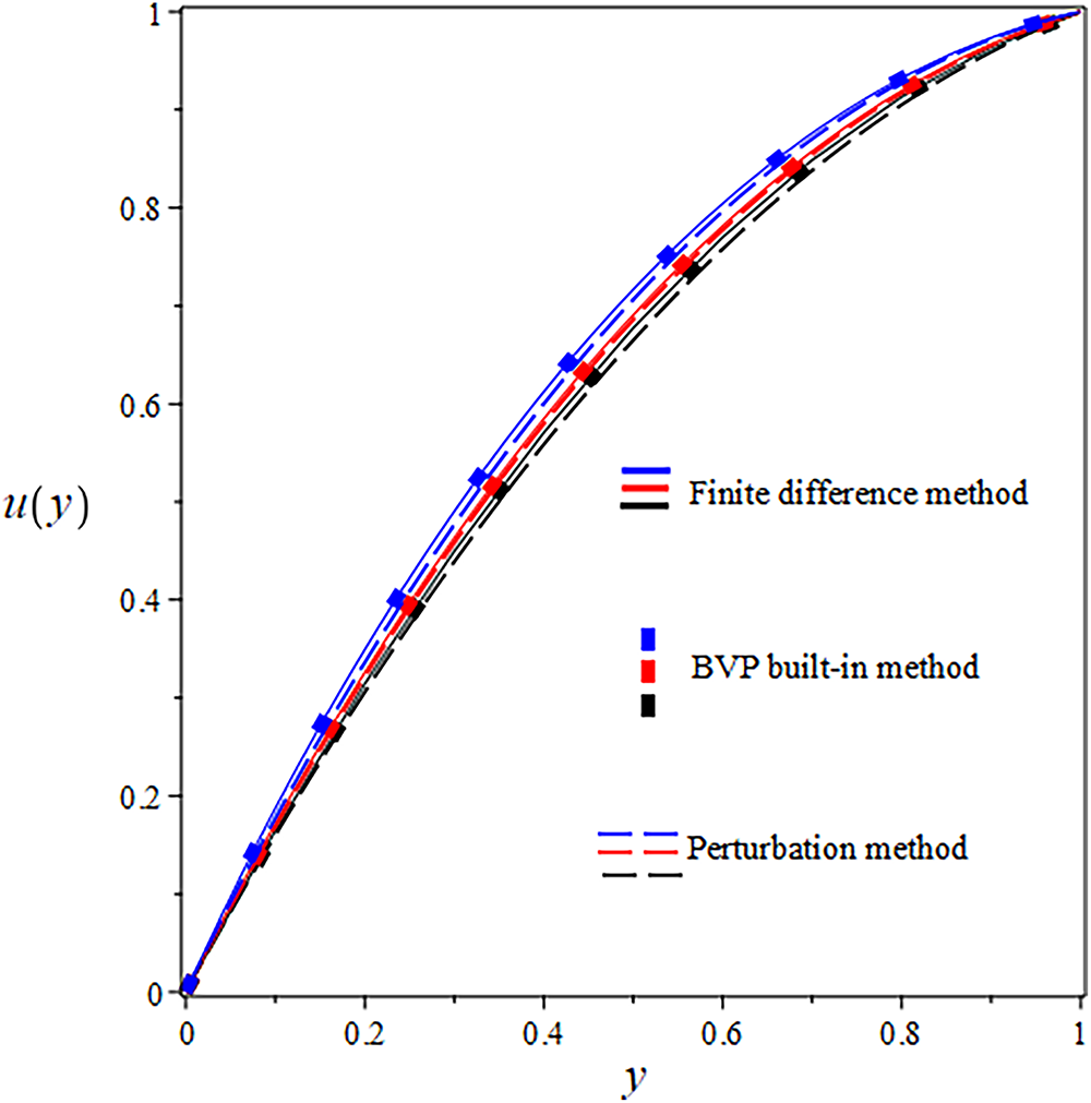
Figure 8: Comparison of
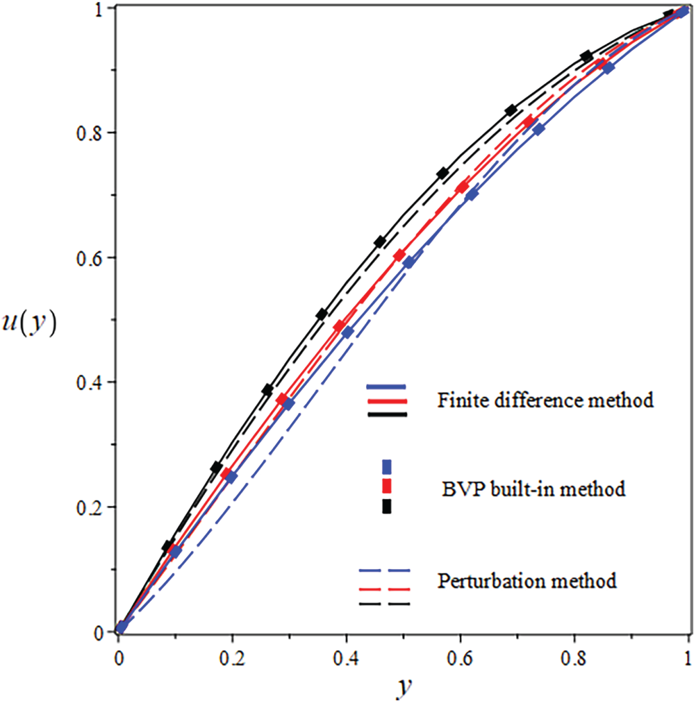
Figure 9: Comparison of
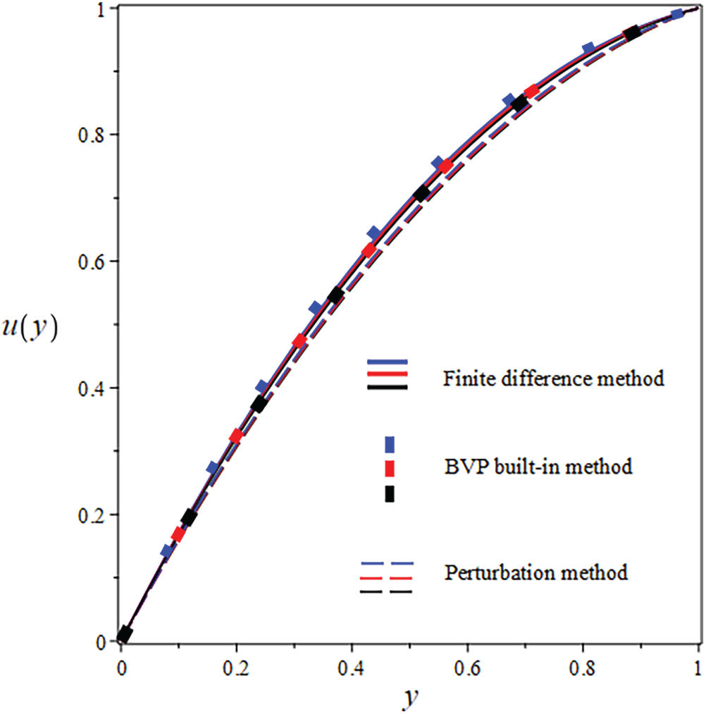
Figure 10: Comparison of
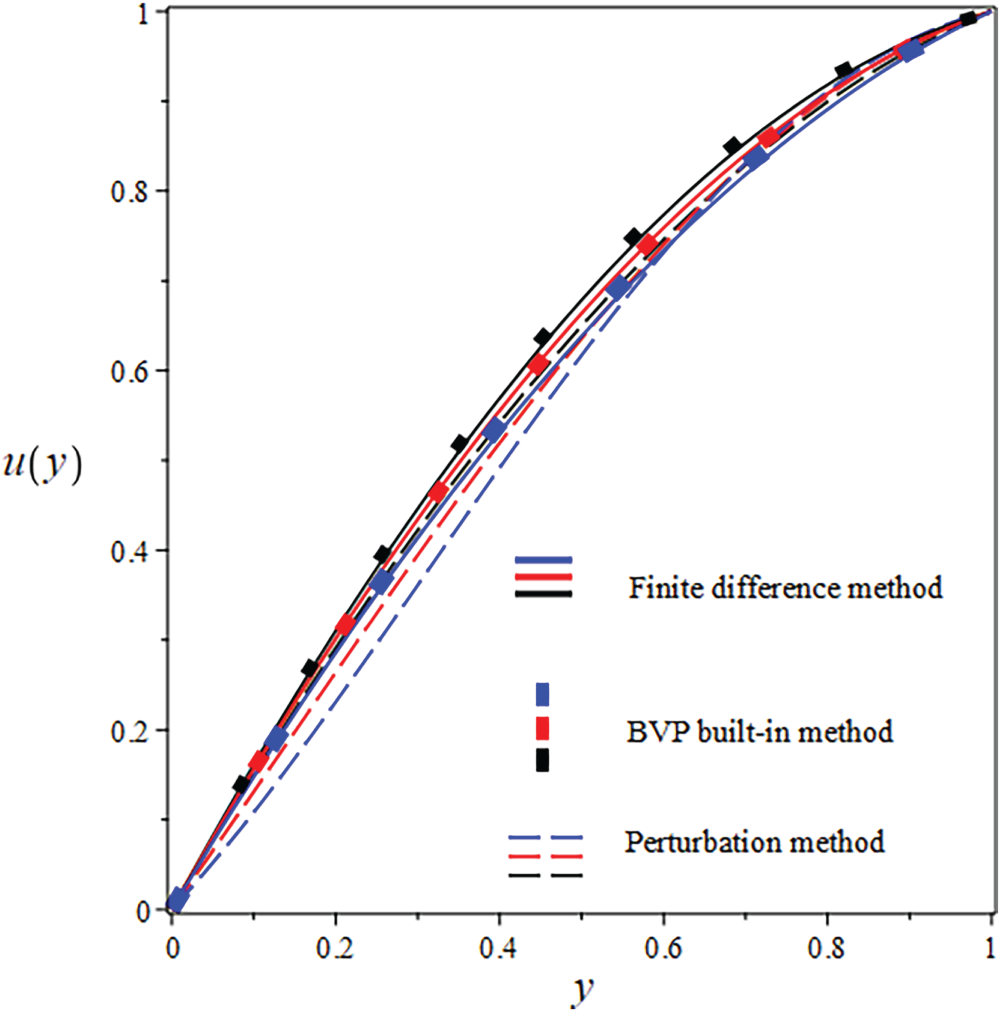
Figure 11: Comparison of
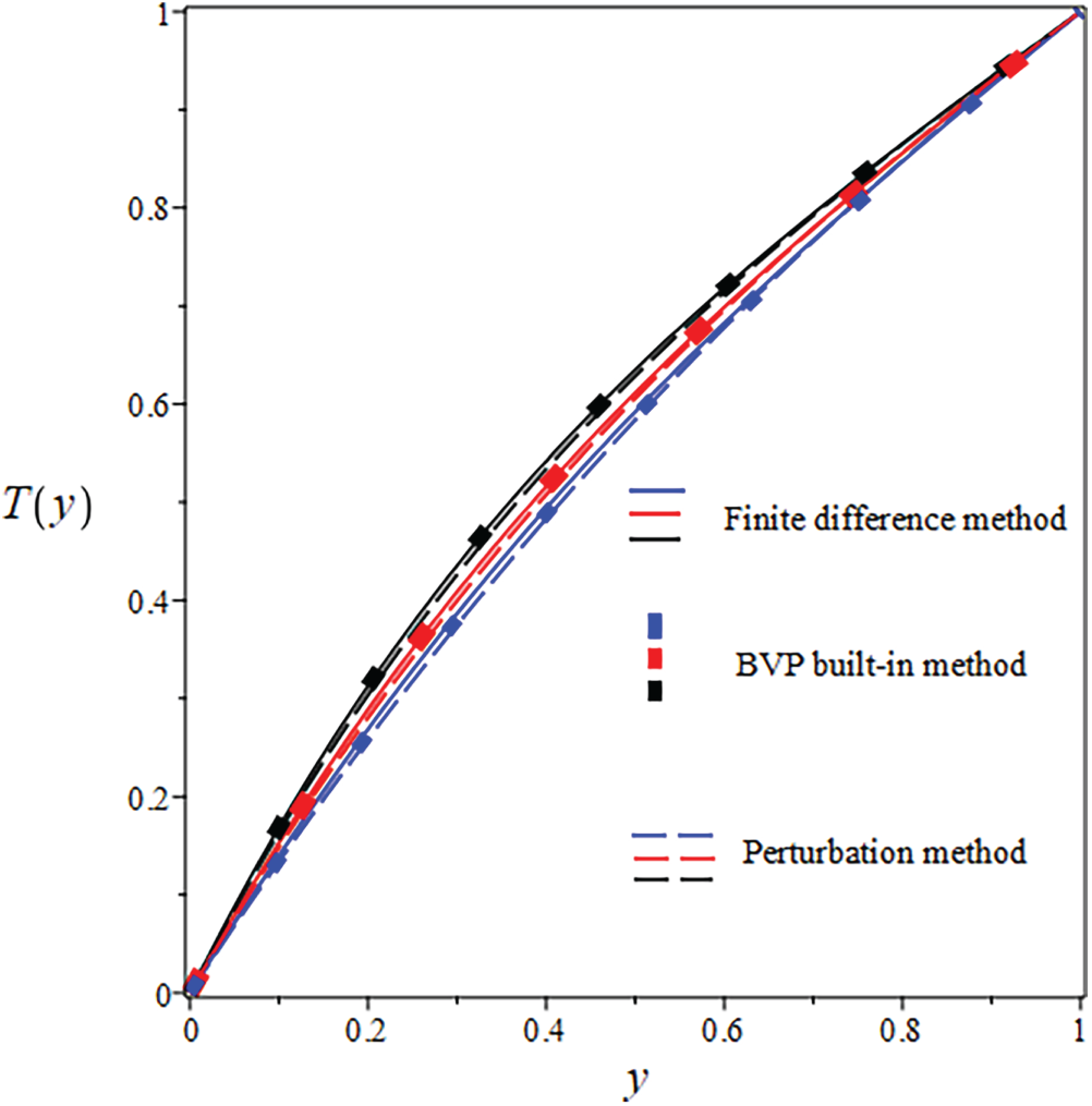
Figure 12: Comparison of
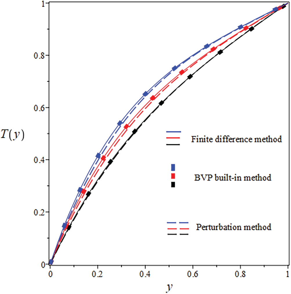
Figure 13: Comparison of
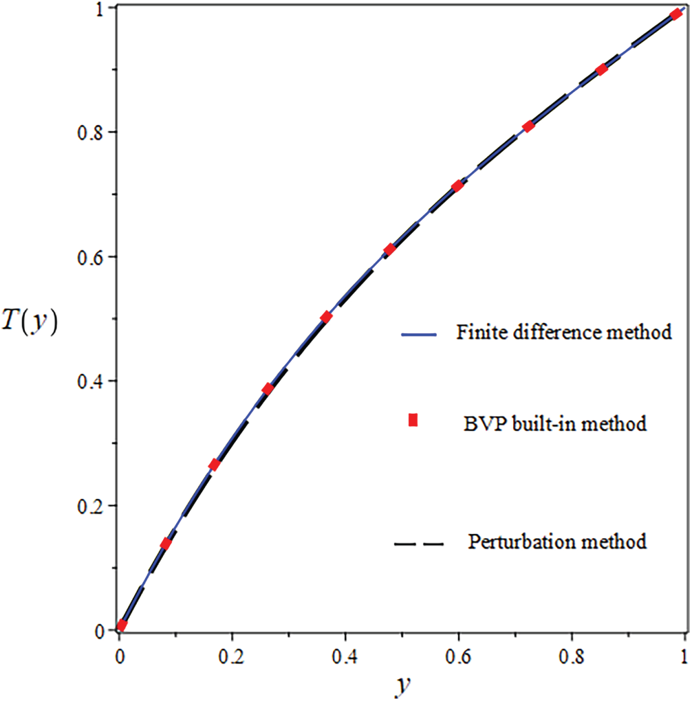
Figure 14: Comparison of
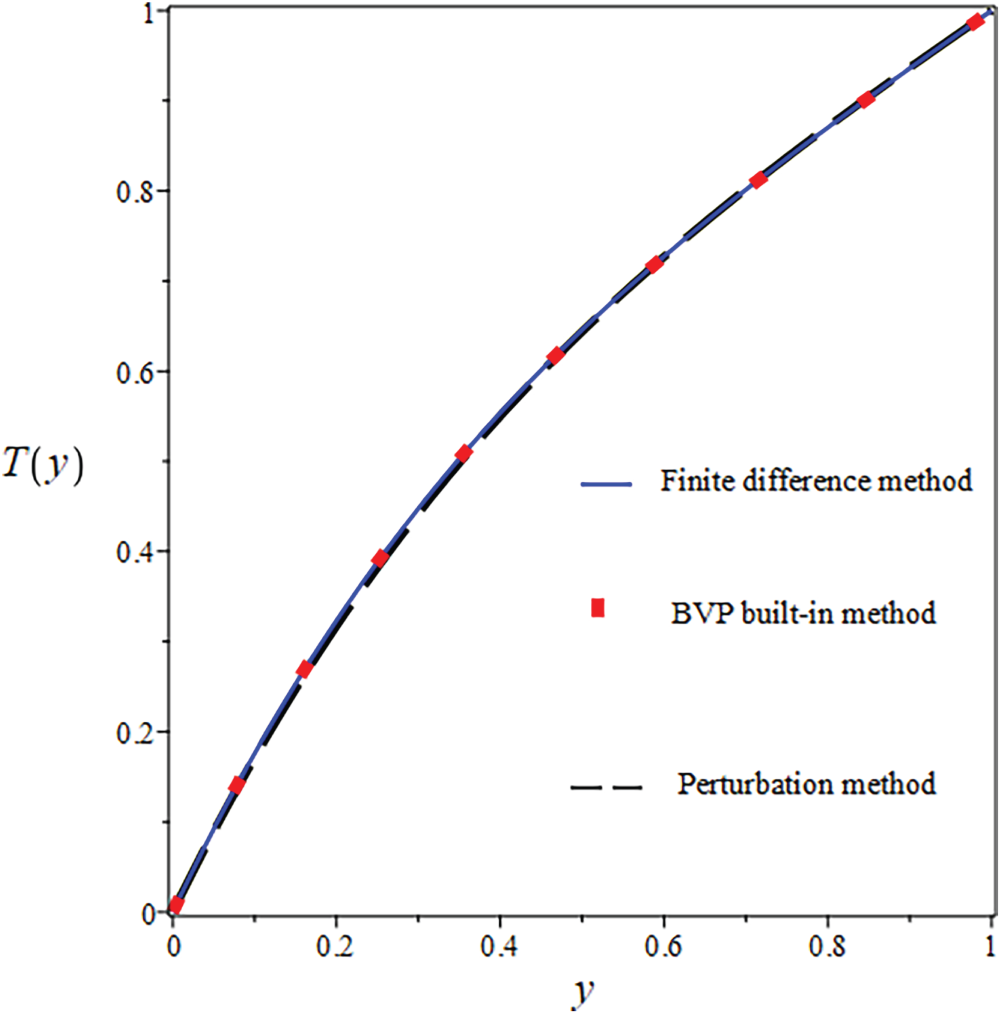
Figure 15: Comparison of
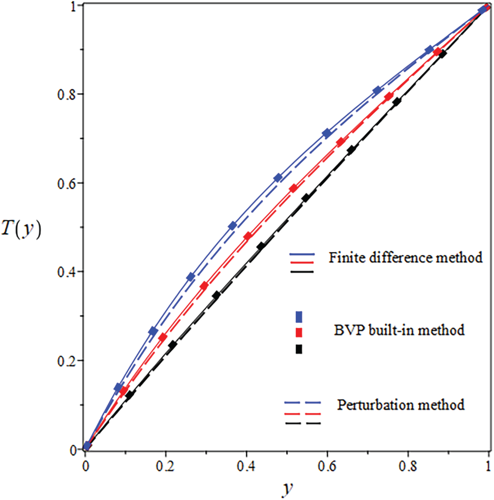
Figure 16: Comparison of
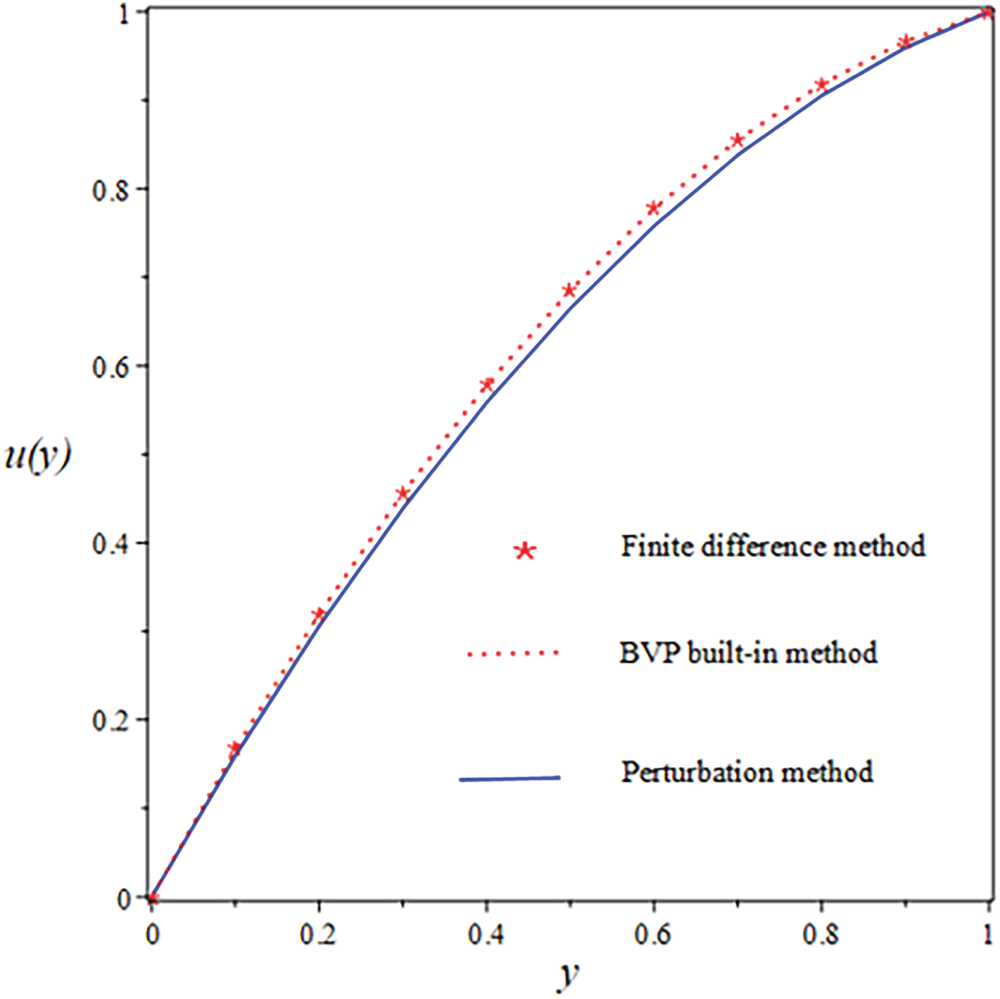
Figure 17: Comparison of errors between analytic and numerical solutions
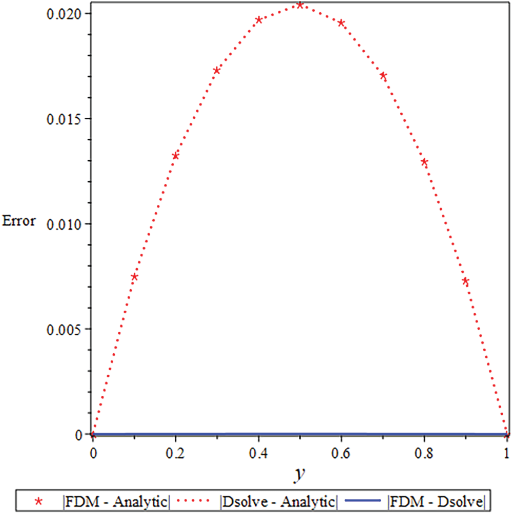
Figure 18: Analysis of the error behavior in the analytical vs. numerical solutions
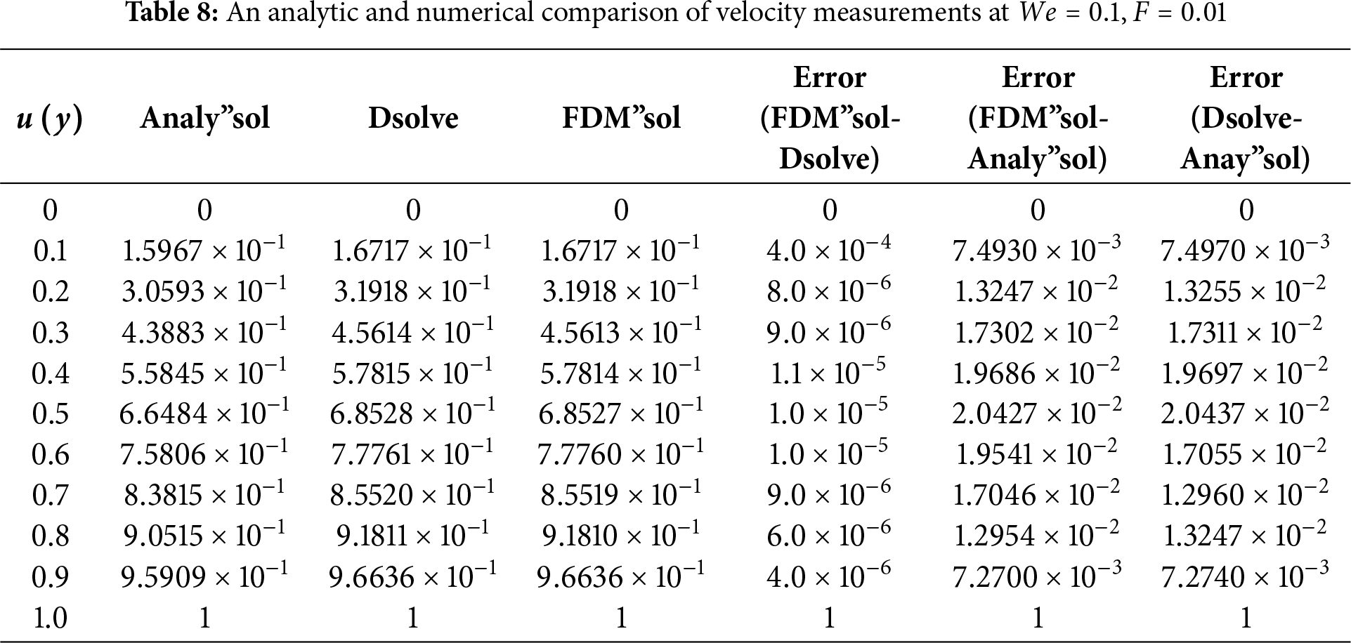
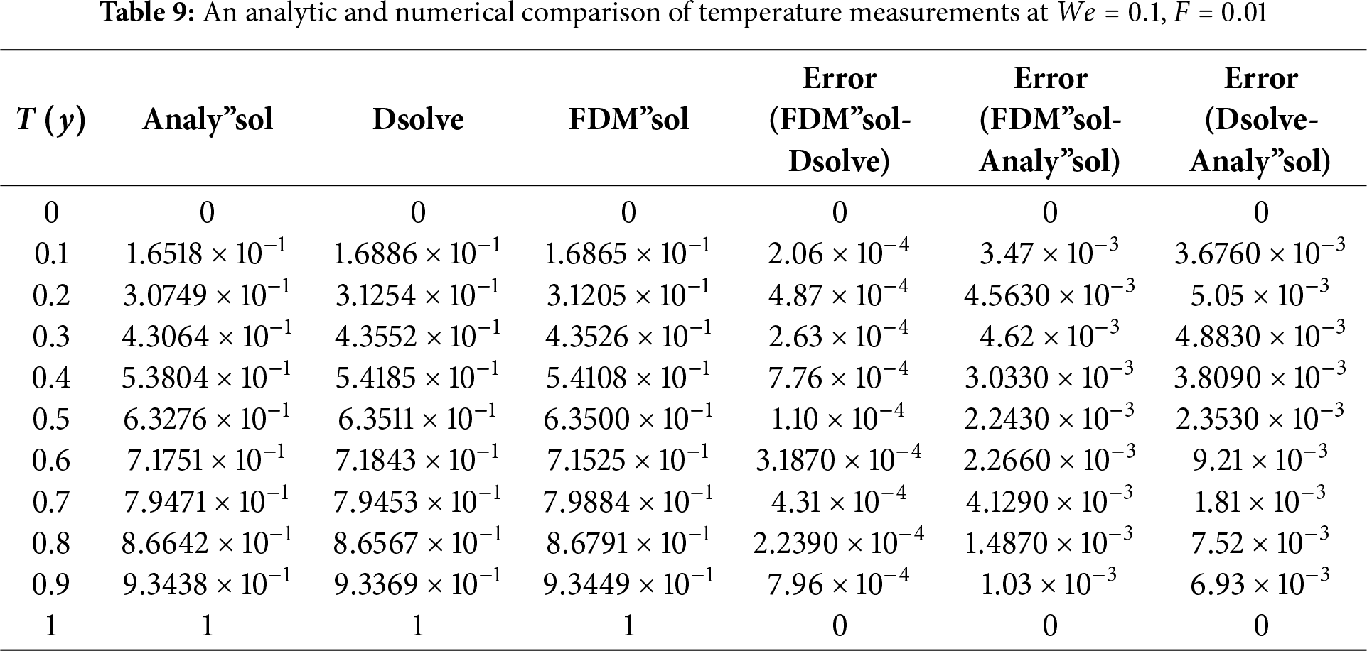
The suggested numerical method yields both the exact and approximate solutions, and the error is visible in both cases. Solid lines indicate FDM findings, solid boxes show results from the integrated BVP approach, and dashed lines show analytical results in the numerical results. The use of numerical and analytical solutions is justified because of their clearly superior performance in terms of accuracy. Three curves, each in black, red, and blue, make up each design. The solutions for one parameter value are shown by the black curve, and the solutions for two more parameter values are shown by the red and blue curves. The visuals demonstrate a robust interrelationship within all proposed solutions. This reinforces confidence in the reliability of all results. Tables 8 and 9 present an analytical and numerical comparison of velocity and temperature measurements at We = 0.1, F = 0.01, and the corresponding absolute errors are also reported. The tables demonstrate a decrease in the absolute error when comparing the analytical and numerical results. It proves the validity of our technique and the related computations. This proves that the methods we used to achieve the results are reliable. The influence of physical characteristics on several important variables will be discussed in the next section using tables and graphs. The analytic and numerical solutions exhibit convergence.
Validation of the Present Model
The accuracy of the present formulation was verified by comparing results with the classical Newtonian model of Middleman [8]. As shown in Figs. 19–22, the velocity, temperature, and pressure profiles show excellent agreement with the established Newtonian data at
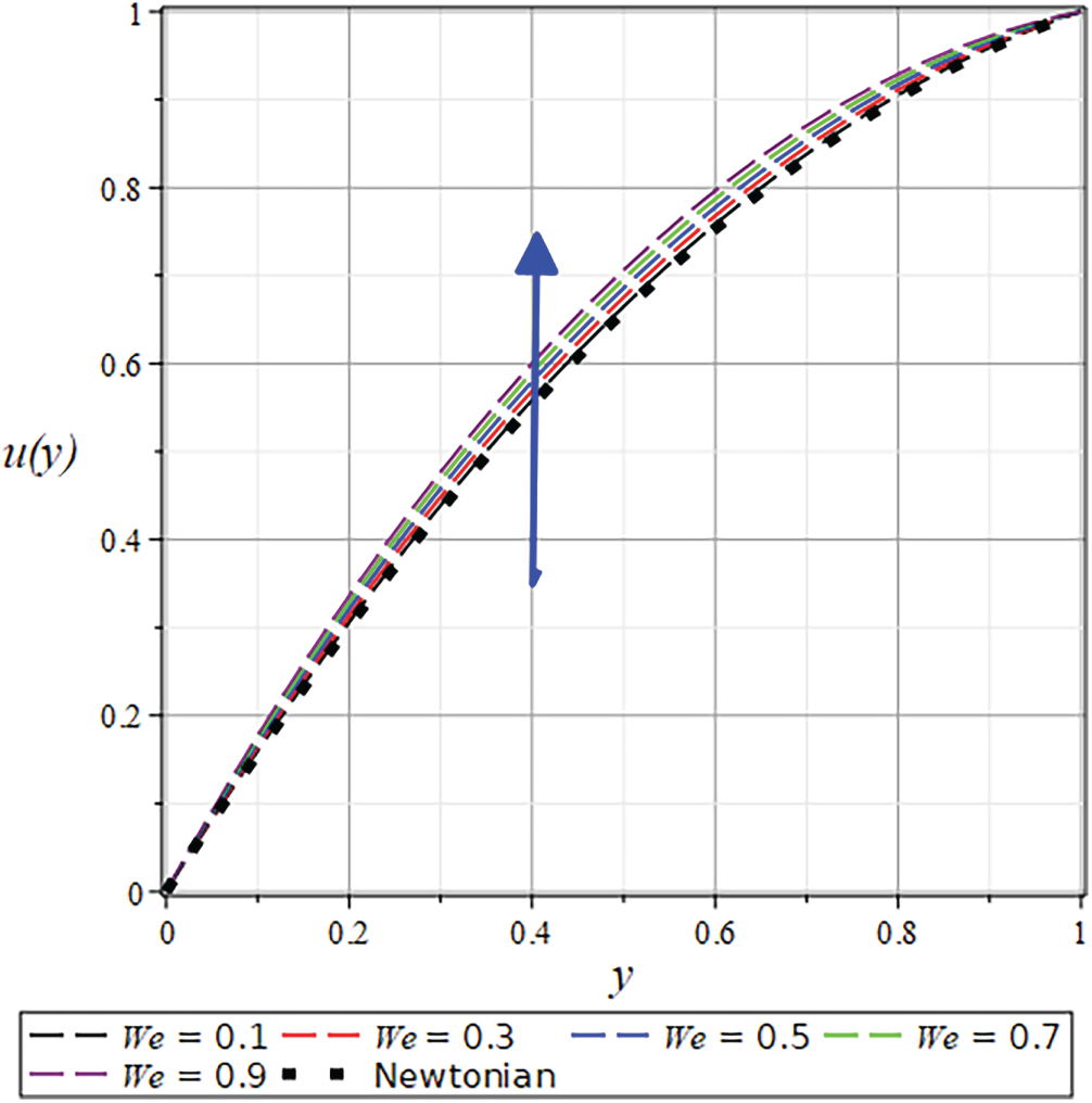
Figure 19: The
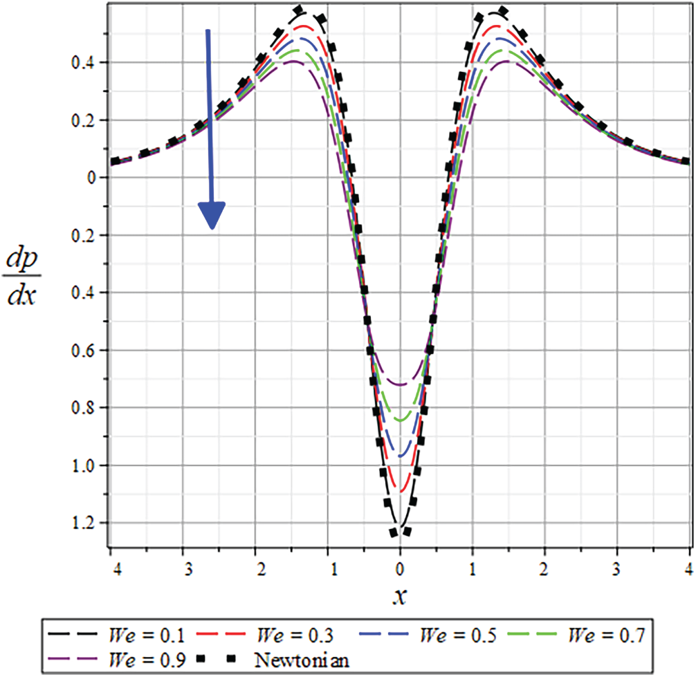
Figure 20: The
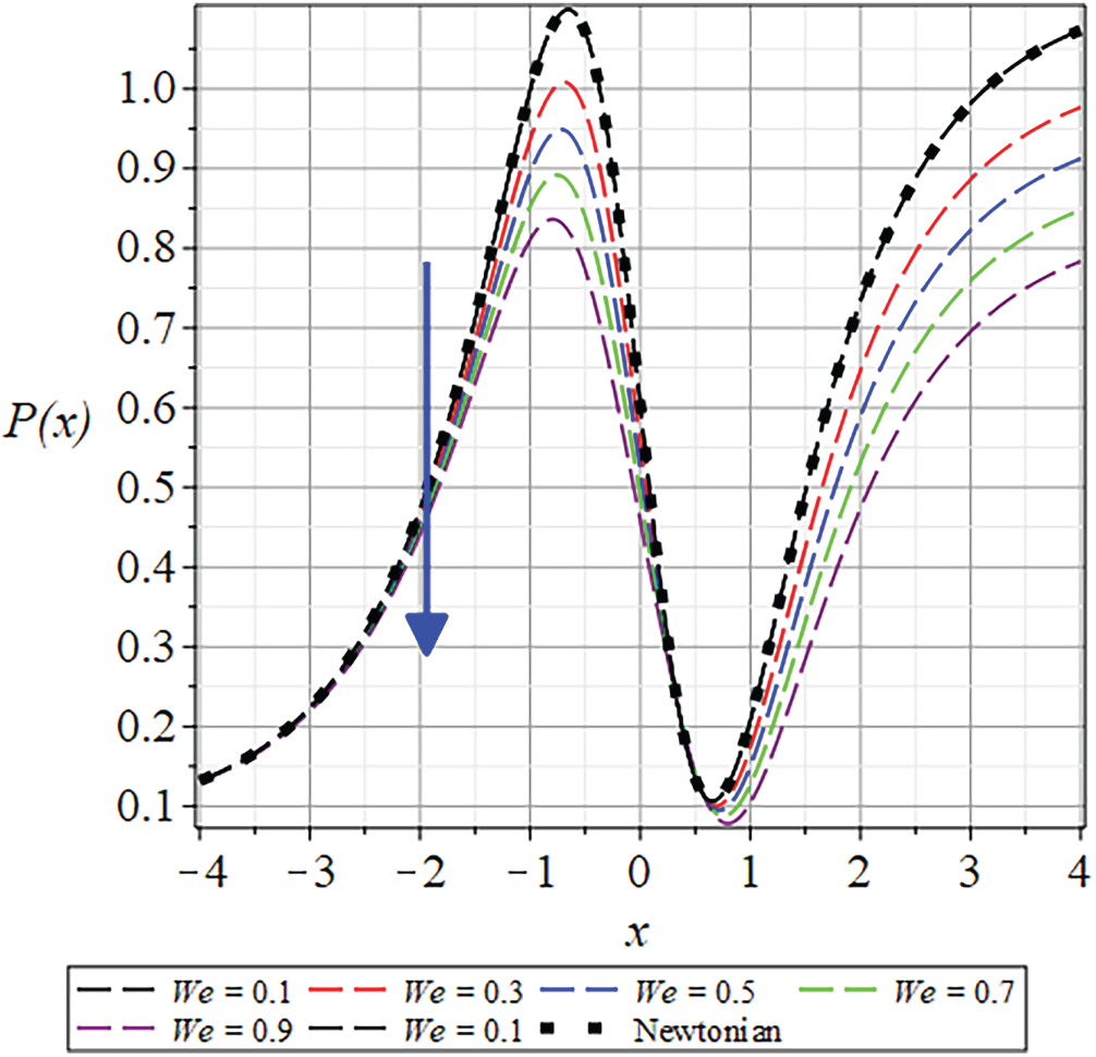
Figure 21: The
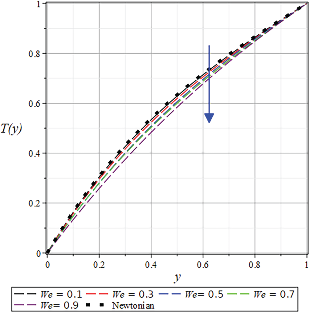
Figure 22: The
The mathematical modeling of CRF flow is analyzed under fixed boundary constraints to establish a rigorous framework for a non-Newtonian, incompressible fluid traversing the narrow gap between the roll and substrate. This study systematically examines the influence of essential governing parameters on the spatial distributions of velocity, pressure, temperature, and other vital engineering variables. The research clarifies the complex relationship between flow dynamics and thermal transport, yielding essential insights into the fundamental physical mechanisms, offering a predictive basis for enhancing CRF processes. The governing equations are simplified with the application of LAT. Closed-form solutions are derived analytically utilizing PM for the velocity profile, the temperature distribution for the pressure distribution, and
Numerous flow parameters are presented through tables and graphical representations. Figs. 19 and 22–38 show how different parameters affect the velocity and temperature of the RC flow. Likewise, Figs. 20, 21, 39 and 40 show the pressure distribution and gradient. Moreover, the results for the
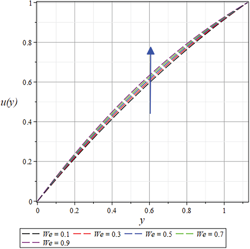
Figure 23: The
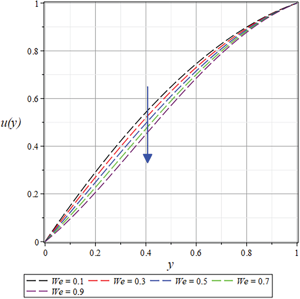
Figure 24: The
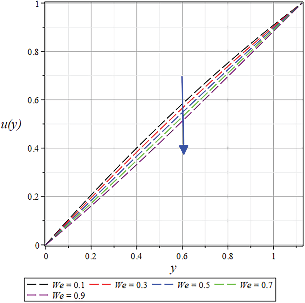
Figure 25: The
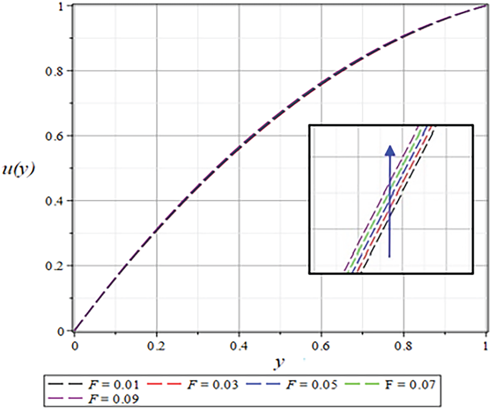
Figure 26: The
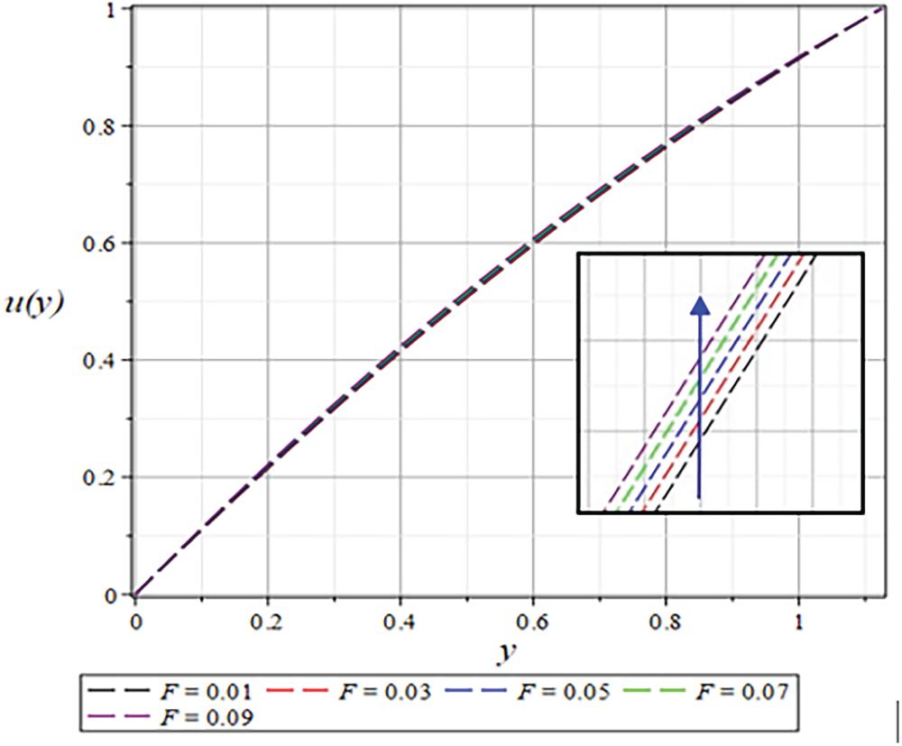
Figure 27: The
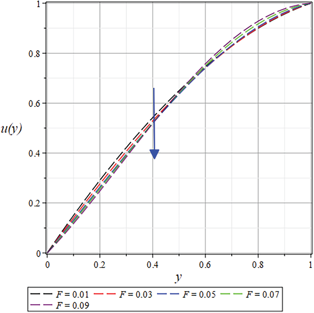
Figure 28: The
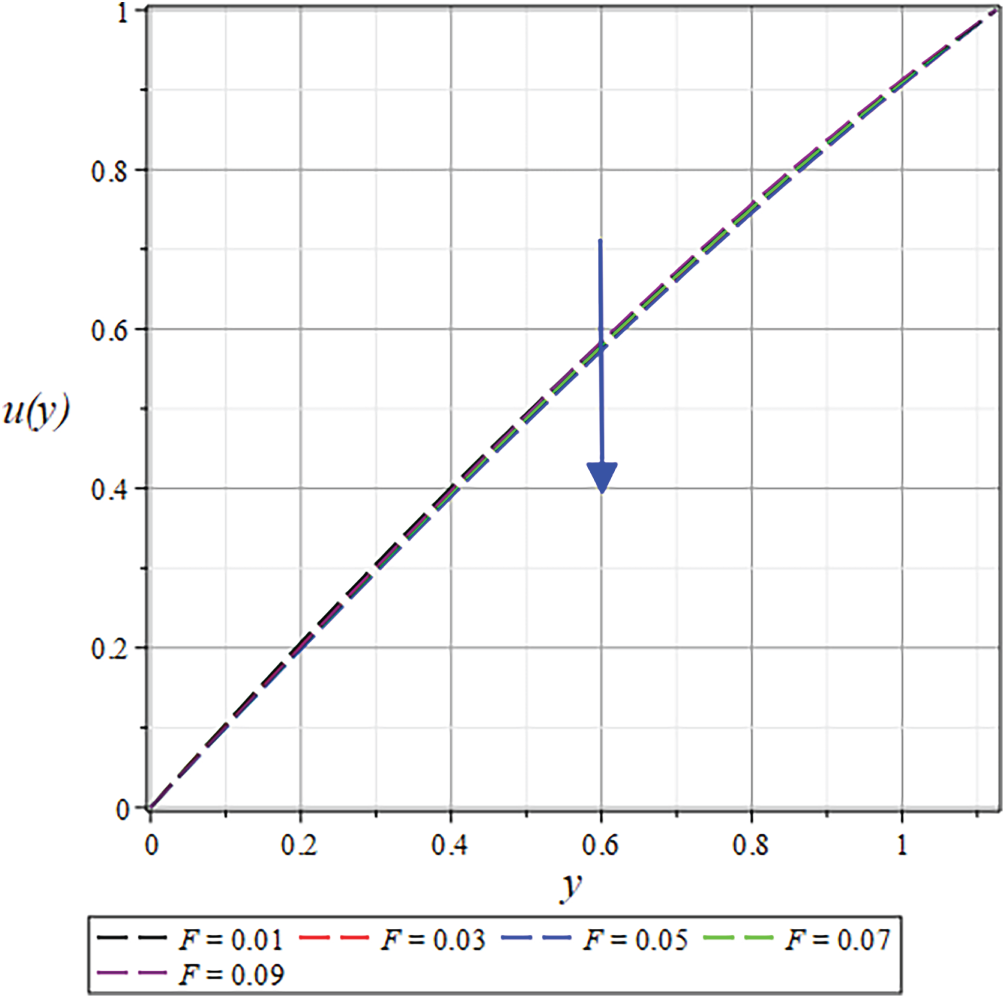
Figure 29: The
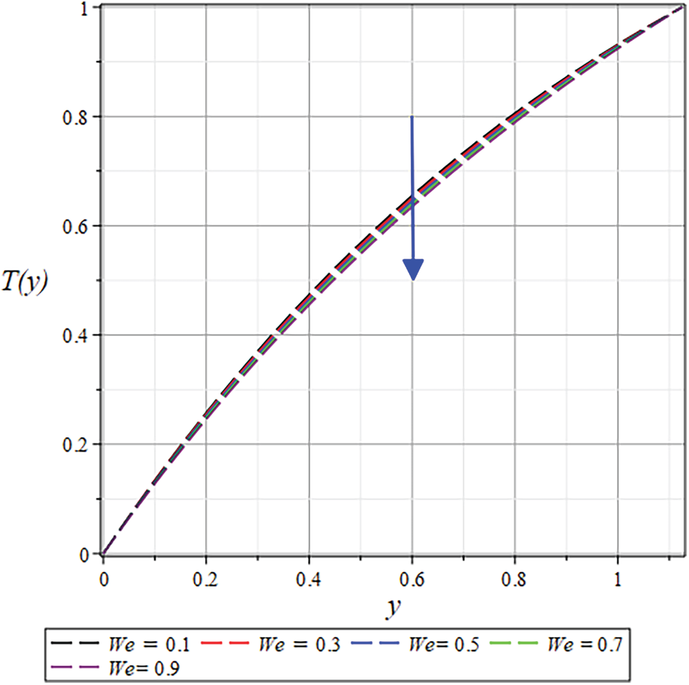
Figure 30: The
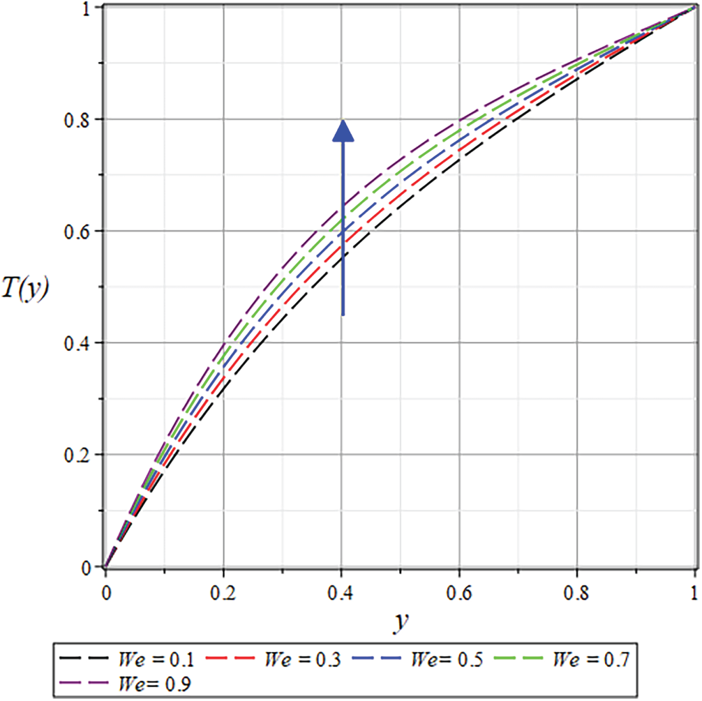
Figure 31: The
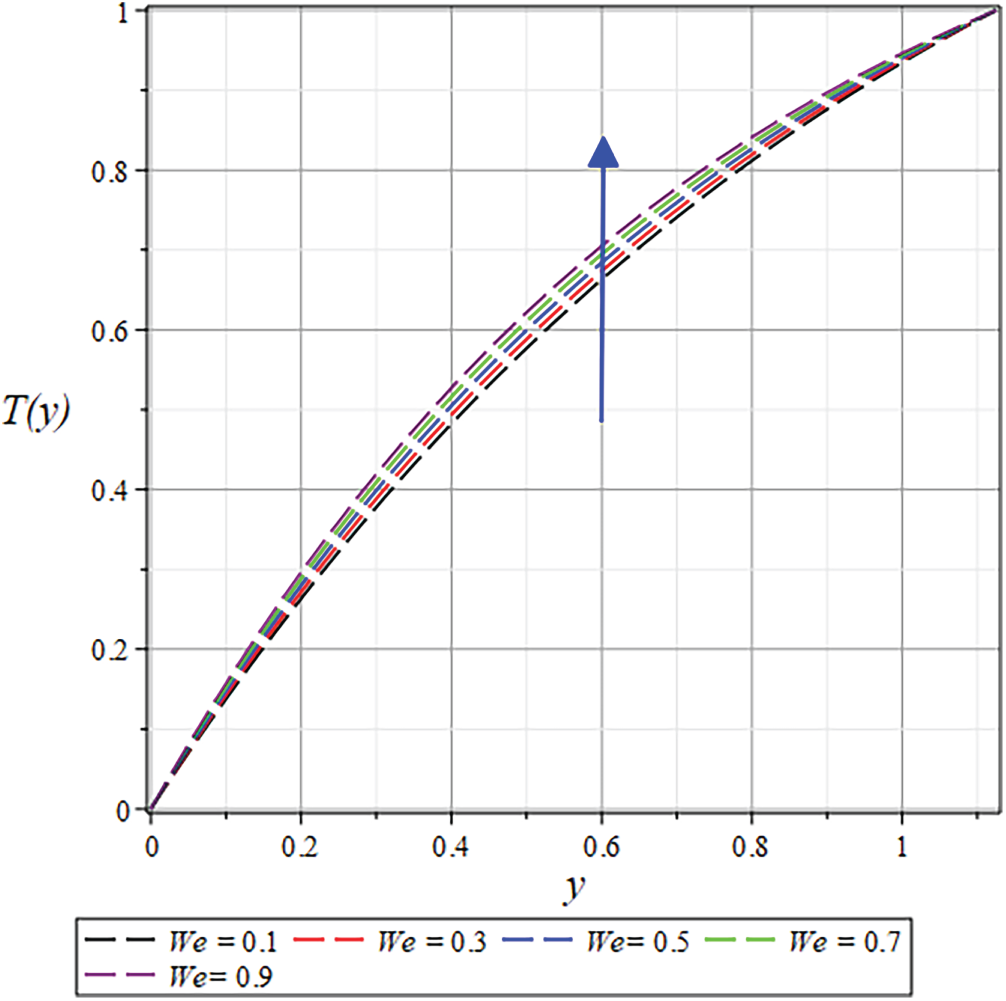
Figure 32: The
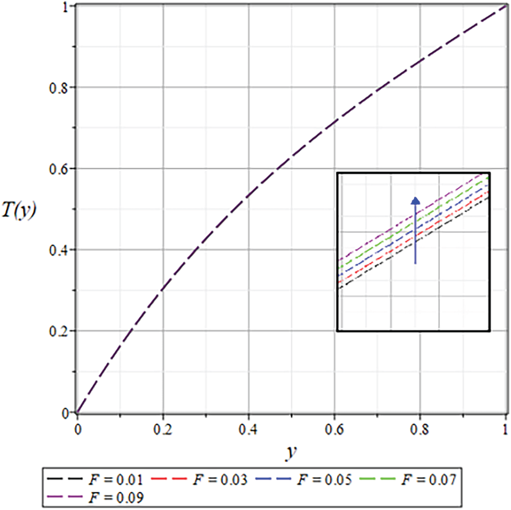
Figure 33: The
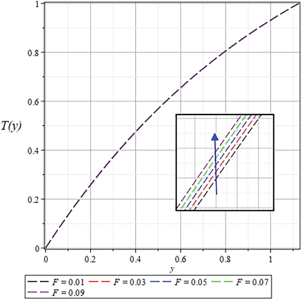
Figure 34: The
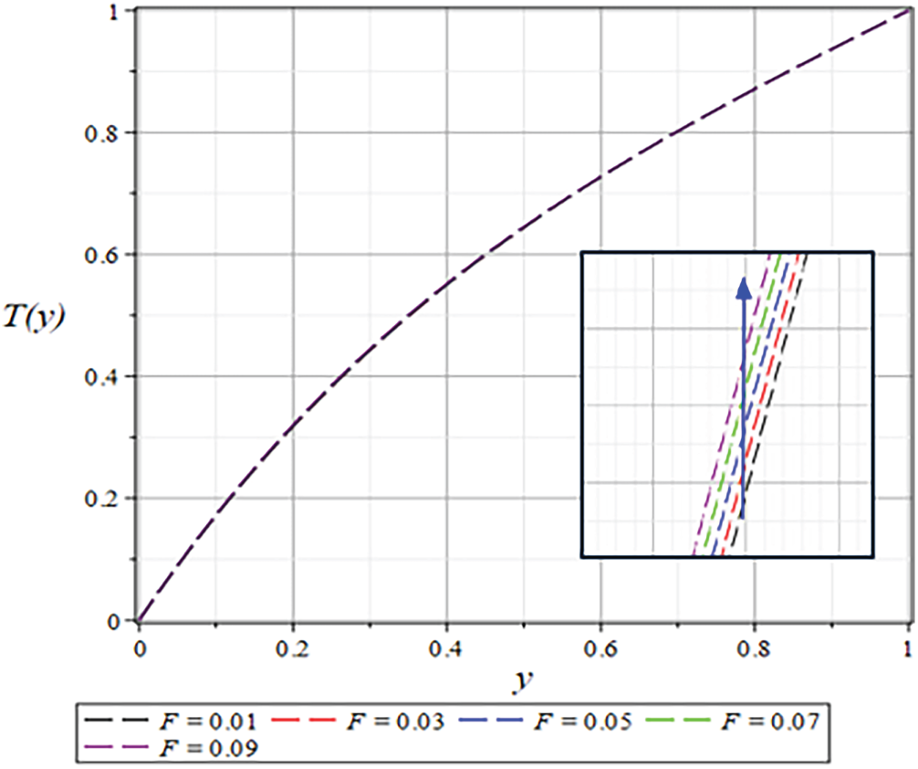
Figure 35: The
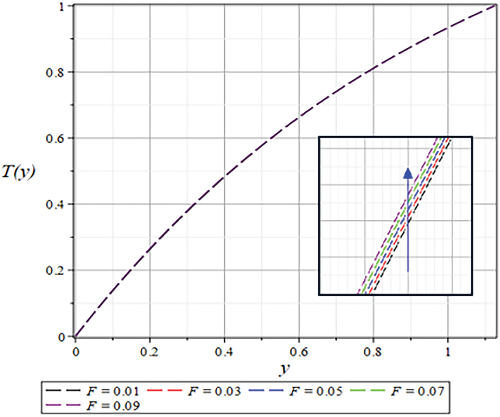
Figure 36: The
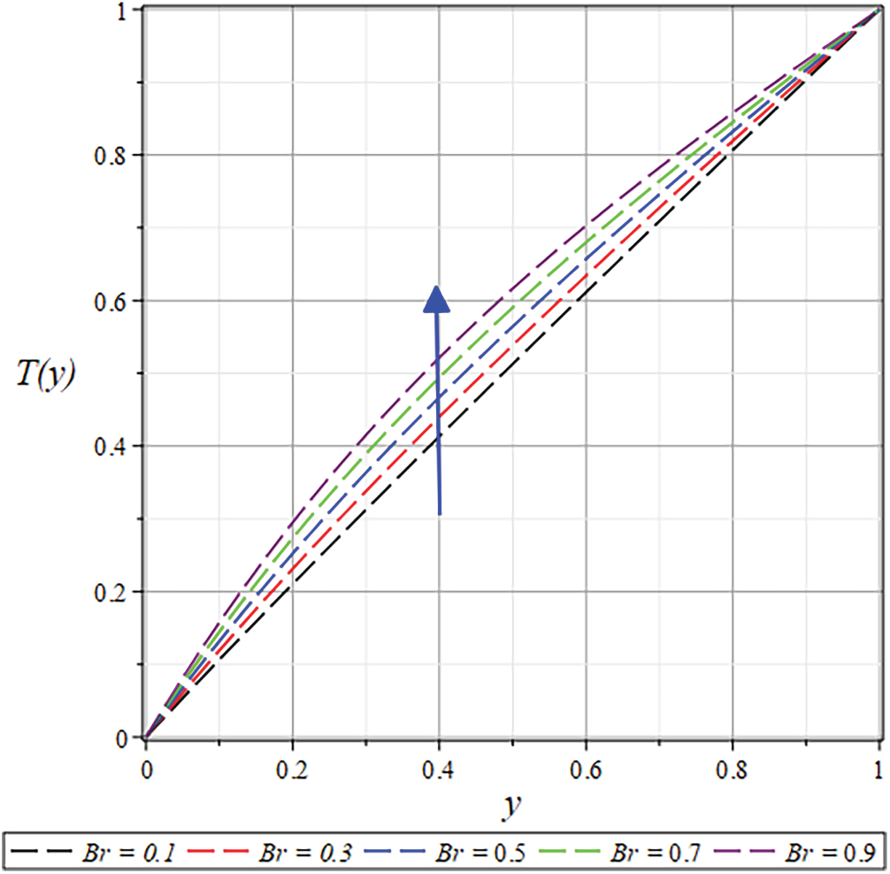
Figure 37: The
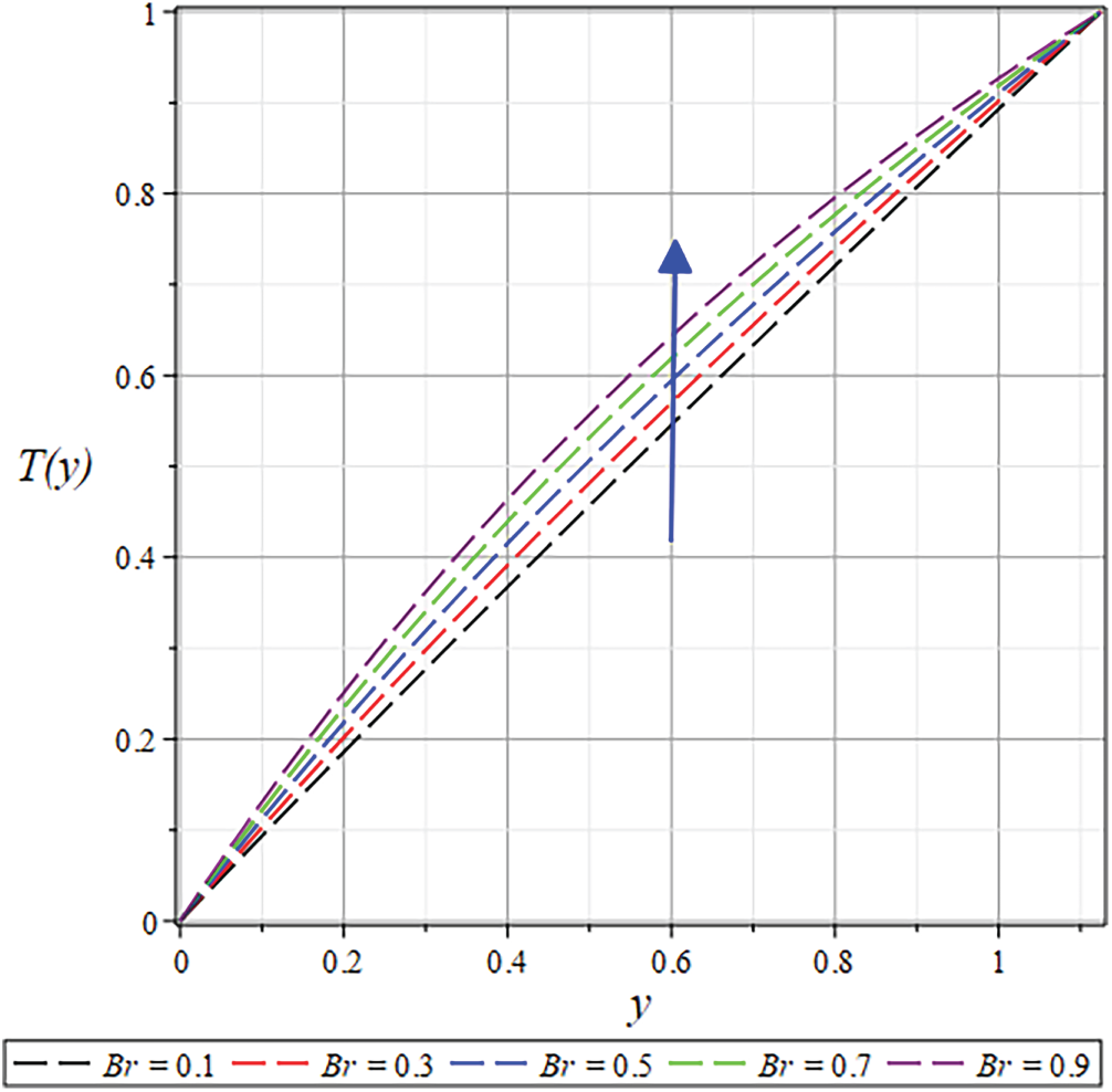
Figure 38: The
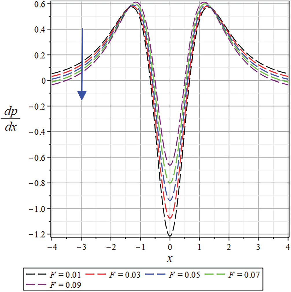
Figure 39: The
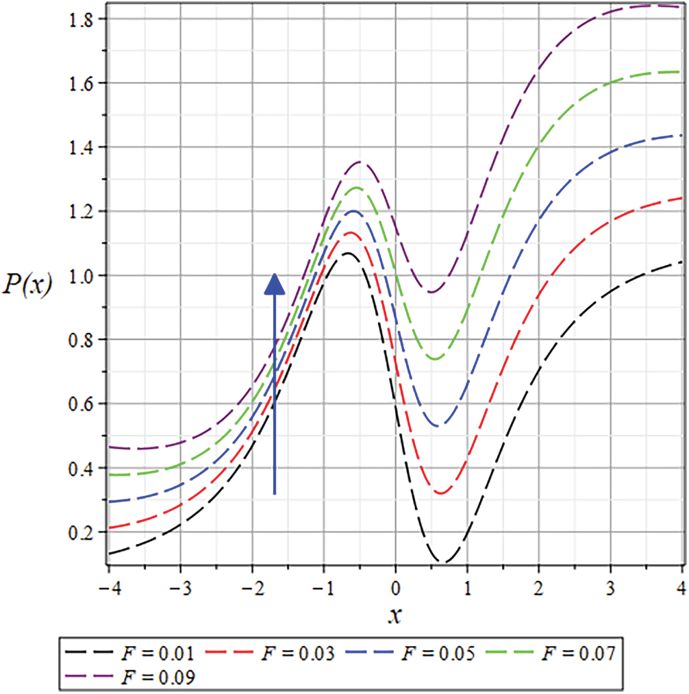
Figure 40: The
A. Velocity profile
The velocity profile shows a significant enhancement with increasing
The results for the dimensionless velocity profiles as a function of
For a shear-thinning fluid (
B. Pressure profile and gradient
The pressure distribution exhibits a strong dependence on rheological parameters, diminishing with increasing
Understanding how parameters like
Figs. 21 and 40 depict the pressure distribution for various values of
C. Temperature profile
The theoretical investigation of the RC procedures for fluids that are non-Newtonian is greatly affected by temperature. Temperature significantly influences the rheological properties of fluids and the coating process as a whole. The temperature distribution is significantly influenced by both rheological and operational parameters. The roll has zero temperature at the edge, but reaches its maximum temperature in the middle. The rise in temperature with increasing
The temperature distribution is observed in Figs. 22 and 30 to decline at various coating process locations with increasing the values of
While an opposite trend is witnessed in Figs. 31 and 32 for
Figs. 37 and 38 illustrate how
Additional quantities of engineering significance, including
D. Streamlines
Streamlines are a fundamental concept in fluid mechanics, describing the path that fluid particles adhere to in a steady flow. They are defined as curves that are consistently tangent to the velocity vector of the flow, indicating that a fluid element traverses along a streamline without intersecting it.
A fundamental attribute of streamlines is their non-intersection, as the velocity at any location in the flow field has a unique direction. The flow behavior of the fluid can be illustrated by creating streamlined patterns. This mathematical formulation ensures the automatic satisfaction of the continuity equation. They illuminate the overall flow structure, encompassing the presence of areas with elevated or diminished velocity. The streamline plots in Figs. 41–44 illustrate that the flow displays symmetry about the vertical

Figure 41: Streamline for

Figure 42: Streamline for
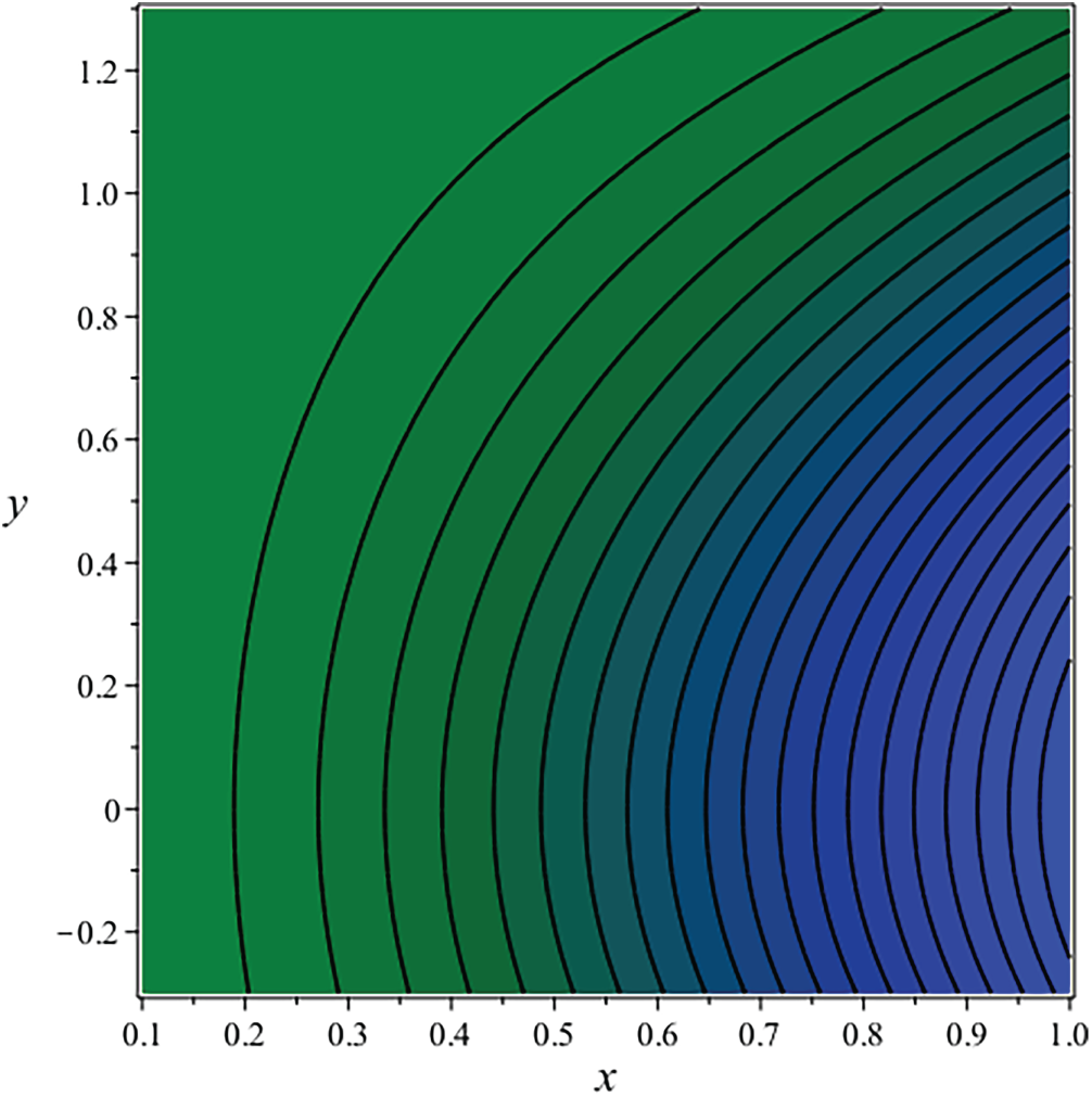
Figure 43: Streamline for
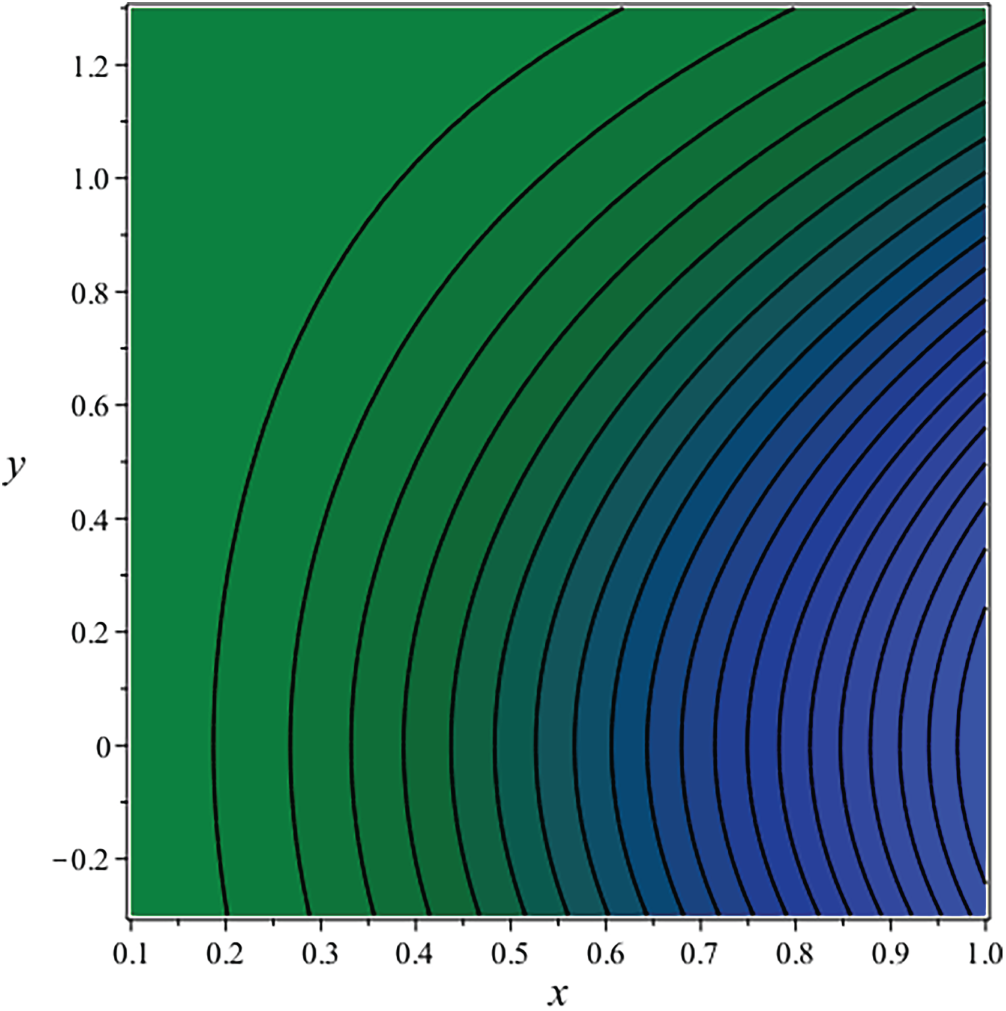
Figure 44: Streamline for
This study effectively addresses a significant gap in the literature by formulating a comprehensive model for non-isothermal Carreau fluid flow in a roll coating process with a fixed constrained wall, a configuration pertinent to industrial thickness control. The primary contributions and engineering results are summarized as follows:
(a) Innovative Modeling and Validation: We developed a novel hybrid analytical-numerical framework for this previously unexplored configuration. The excellent agreement between our perturbation solutions and numerical results (FDM, BVP), as vividly demonstrated in Figs. 8–18, confirms the robustness and accuracy of our model. Furthermore, Figs. 19–22 validate our approach by showing perfect agreement with the classical Newtonian model for the limiting case
(b) Key Engineering Outcomes and Design Guidance: The parametric analysis, illustrated through extensive figures, provides direct design insights:
Coating Thickness Control: Figs. 19 and 23 show that for shear-thinning fluids
Energy and Load Management: Figs. 20, 21, 39 and 40 reveal that pressure and separation force can be managed by tuning
Thermal Management: Figs. 22 and 30–38 indicate that temperature rises with the
(c) Practical Optimization Framework: We employed Response Surface Methodology (RSM) to transform our findings into a practical optimization tool. The high coefficients of determination Table 6 and the clear trends in the 3-D response surfaces (Fig. 4) allow engineers to identify the optimal combination of
(d) Future work and its applicability: In the future, we will be able to validate this study for a variety of engineering studies, both experimental and theoretical, that include complex structures. (Newtonian and non-Newtonian fluids) by applying slip/no-slip, MHD, and many other fluid properties. We will extend the present model to multi-dimensional and transient analyses using advanced numerical methods and integrate machine learning for faster and more accurate predictions. The extended model will help optimize coating thickness, flow uniformity, and heat transfer in practical non-Newtonian roll-coating systems.
(e) Limitations of the Present Study: Although the present study establishes a comprehensive analytical-numerical framework for non-isothermal Carreau fluid flow in roll coating with a fixed constrained wall, several inherent limitations remain. The formulation relies on the lubrication approximation and assumes a thin, steady, laminar film with predominantly unidirectional flow, which may not fully capture high-speed or inertia-dominated coating conditions. The perturbation methodology is applicable only for small
In summary, this paper provides a validated theoretical mode, along with explicit directions and a practical framework for optimizing industrial roll coating processes. The results indicate that by strategically choosing the fluid’s rheological characteristics (shear-thinning behavior) and operating conditions (moderate to high
Acknowledgement: Not applicable.
Funding Statement: This study is supported by the Talent Project of Tianchi Young-Doctoral Program in Xinjiang Uygur Autonomous Region of China (No. 51052401510), and Natural Science Foundation General Project (Grant Number 2025D01C36) of the Xinjiang Uyghur Autonomous Region of China. Also, This study received financial support from the National Natural Science Foundation of Xinjiang Province (Grant Nos. 2022TSYCTD0019 and 2022D01D32), the China Scholarship Council (CSC) (Grant No. 2021SLJ009915).
Author Contributions: The concept was developed by Fateh Ali, M. Zahid and Mujahid Islam, and subsequently incorporated into a mathematical model by Mujahid Islam and Fateh Ali. The problem was solved by Mujahid Islam. The manuscript was drafted by Fateh Ali, Xinlong Feng and Sana Naz Maqbool, with supervision provided by Xinlong Feng. Mujahid Islam and Fateh Ali analyzed the underlying physics and contributed to the discussion. Finally, Xinlong Feng and M. Zahid reviewed, edited, and assisted with English language corrections. All authors reviewed the results and approved the final version of the manuscript.
Availability of Data and Materials: Relevant data for this study are accessible from the corresponding authors upon reasonable inquiry.
Ethics Approval: Not applicable.
Conflicts of Interest: The authors declare no conflicts of interest to report regarding the present study.
Nomenclature
| Roman Letters | |
| Velocity components in | |
| Specific Heat capacity | |
| Dimensionless gravity parameter | |
| Roll separation force | |
| Gravitational acceleration constant | |
| Coating thickness | |
| Identity tensor | |
| Power law index | |
| Pressure | |
| Power input | |
| Temperature | |
| Rivlin Erickson tensor | |
| Velocity field | |
| Velocity gradient | |
| Half of the nip region | |
| Separation point | |
| Reynolds number | |
| Wiesenberger number | |
| Brickman number | |
| Eckert number | |
| Prandtl number | |
| Nusselt number | |
| Greek Letters | |
| Stress tensor | |
| Fluid elasticity | |
| Shear rate | |
| Coating thickness | |
| Viscosity | |
| Infinite shear-rate viscosities | |
| Zero shear-rate viscosities | |
| Fluid density | |
References
1. Hermia J. Blocking filtration. application to non-Newtonian fluids. In: Mathematical models and design methods in solid-liquid separation. Berlin/Heidelberg, Germany: Springer; 1985. p. 83–9. doi:10.1007/978-94-009-5091-7_5. [Google Scholar] [CrossRef]
2. Awais M, Salahuddin T, Muhammad S. Evaluating the thermo-physical characteristics of non-Newtonian Casson fluid with enthalpy change. Therm Sci Eng Prog. 2023;42:101948. doi:10.1016/j.tsep.2023.101948. [Google Scholar] [CrossRef]
3. Toghraie D, Esfahani NN, Zarringhalam M, Shirani N, Rostami S. Blood flow analysis inside different arteries using non-Newtonian Sisko model for application in biomedical engineering. Comput Meth Programs Biomed. 2020;190:105338. doi:10.1016/j.cmpb.2020.105338. [Google Scholar] [PubMed] [CrossRef]
4. Liu TJ, Lin HM, Hong CN. Comparison of two numerical methods for the solution of non-Newtonian flow in ducts. Num Meth Fluids. 1988;8(7):845–61. doi:10.1002/fld.1650080707. [Google Scholar] [CrossRef]
5. Yasir M, Ahmed A, Khan M, Ch MMI, Ayub M. Study on time-dependent Oldroyd-B fluid flow over a convectively heated surface with Cattaneo-Christov theory. Waves Random Complex Medium. 2025;35(1):144–61. doi:10.1080/17455030.2021.2021316. [Google Scholar] [CrossRef]
6. Nayfeh AH. Perturbation methods. Hoboken, NJ, USA: John Wiley & Sons; 2024. [Google Scholar]
7. Coyle DJ. The fluid mechanics of roll coating: steady flows, stability, and rheology. Minneapolis, MN, USA: University of Minnesota; 1984. [Google Scholar]
8. Sullivan TM, Middleman S. Roll coating in the presence of a fixed constraining boundary. Chem Eng Commun. 1979;3(6):469–82. doi:10.1080/00986447908935879. [Google Scholar] [CrossRef]
9. Greener Y, Middleman S. Blade-coating of a viscoelastic fluid. Polym Eng Sci. 1974;14(11):791–6. doi:10.1002/pen.760141110. [Google Scholar] [CrossRef]
10. Hintermaier J, White R. The splitting of a water film between rotating rolls. Tappi J. 1965;48(11):617–25. [Google Scholar]
11. Greener J, Middleman S. Reverse roll coating of viscous and viscoelastic liquids. Ind Eng Chem Fund. 1981;20(1):63–6. doi:10.1021/i100001a012. [Google Scholar] [CrossRef]
12. Owens MS, Vinjamur M, Scriven LE, Macosko CW. Misting of non-Newtonian liquids in forward roll coating. J Non Newton Fluid Mech. 2011;166(19–20):1123–8. doi:10.1016/j.jnnfm.2011.06.008. [Google Scholar] [CrossRef]
13. Lécuyer HA, Mmbaga JP, Hayes RE, Bertrand FH, Tanguy PA. Modelling of forward roll coating flows with a deformable roll: application to non-Newtonian industrial coating formulations. Comput Chem Eng. 2009;33(9):1427–37. doi:10.1016/j.compchemeng.2009.04.001. [Google Scholar] [CrossRef]
14. Ascanio G, Carreau PJ, Tanguy PA. High-speed roll coating with complex rheology fluids. Exp Fluids. 2006;40(1):1–14. doi:10.1007/s00348-005-0025-5. [Google Scholar] [CrossRef]
15. Echendu SOS. Computational and rheological studies for coating flows. Swansea, UK: Swansea University; 2013. [Google Scholar]
16. Raske N, Hewson RW, Kapur N, de Boer GN. A predictive model for discrete cell gravure roll coating. Phys Fluids. 2017;29(6):062101. doi:10.1063/1.4984127. [Google Scholar] [CrossRef]
17. Abdal S, Taha T, Ali L, Zulqarnain RM, Yook SJ. Neural networking-based approach for examining heat transfer and bioconvection in non-Newtonian fluid with chemical reaction over a stretching sheet. Case Stud Therm Eng. 2025;69:106047. doi:10.1016/j.csite.2025.106047. [Google Scholar] [CrossRef]
18. Rajagopal KR. Mechanics of non-Newtonian fluids. In: Recent developments in theoretical fluid mechanics. Boca Raton, FL, USA: Chapman and Hall/CRC; 2023. p. 129–62. doi:10.1201/9781003417026-5. [Google Scholar] [CrossRef]
19. Shahzad MH, Nadeem S, Awan AU, Allahyani SA, Ameer Ahammad N, Eldin SM. On the steady flow of non-Newtonian fluid through multi-stenosed elliptical artery: a theoretical model. Ain Shams Eng J. 2024;15(1):102262. doi:10.1016/j.asej.2023.102262. [Google Scholar] [CrossRef]
20. Khaliq S, Abbas Z. Analysis of calendering process of non-isothermal flow of non-Newtonian fluid: a perturbative and numerical study. J Plast Film Sheeting. 2021;37(3):338–66. doi:10.1177/8756087920979024. [Google Scholar] [CrossRef]
21. Jang J-Y, Chen P-Y. Reverse roll coating flow with non-Newtonian fluids. Commun Comput Phys. 2009;6(3):536. [Google Scholar]
22. Shahzad H, Wang X, Hafeez MB, Shah Z, Alshehri AM. Study of slip effects in reverse roll coating process using non-isothermal couple stress fluid. Coatings. 2021;11(10):1249. doi:10.3390/coatings11101249. [Google Scholar] [CrossRef]
23. Devisetti SK, Bousfield DW. Fluid absorption during forward roll coating of porous webs. Chem Eng Sci. 2010;65(11):3528–37. doi:10.1016/j.ces.2010.02.042. [Google Scholar] [CrossRef]
24. Bhatti MM, Ellahi R, Sait SM. Numerical investigation of magnetized nanofluid flow in a non-Darcian medium with convective heating conditions across a rotating disk. Int J Numer Meth Heat Fluid Flow. 2025;35(5):1736–63. doi:10.1108/hff-03-2025-0135. [Google Scholar] [CrossRef]
25. Farooq A, Rehman S, Ma WX. Comparative study of regression-based data-driven models for thermally stratified Carreau nanofluids with magnesium oxide nanoparticles. Phys Fluids. 2025;37(8):082032. doi:10.1063/5.0274063. [Google Scholar] [CrossRef]
26. Anderson MJ, Whitcomb PJ. RSM simplified: optimizing processes using response surface methods for design of experiments. Boca Raton, FL, USA: Productivity Press; 2016. [Google Scholar]
27. Milani Shirvan K, Mamourian M, Mirzakhanlari S, Ellahi R. Two phase simulation and sensitivity analysis of effective parameters on combined heat transfer and pressure drop in a solar heat exchanger filled with nanofluid by RSM. J Mol Liq. 2016;220:888–901. doi:10.1016/j.molliq.2016.05.031. [Google Scholar] [CrossRef]
28. Greener J, Middleman S. Theoretical and experimental studies of the fluid dynamics of a two-roll coater. Ind Eng Chem Fund. 1979;18(1):35–41. doi:10.1021/i160069a009. [Google Scholar] [CrossRef]
29. Ali F, Hou Y, Feng X, Odeyemi JK, Zahid M, Hussain S. Optimization and sensitivity analysis of heat transfer for Powell-Eyring fluid between rotating rolls with temperature-dependent viscosity: a mathematical modeling approach. Phys Fluids. 2024;36(5):053110. doi:10.1063/5.0211313. [Google Scholar] [CrossRef]
30. Park J, Shin K, Lee C. Roll-to-roll coating technology and its applications: a review. Int J Precis Eng Manuf. 2016;17(4):537–50. doi:10.1007/s12541-016-0067-z. [Google Scholar] [CrossRef]
31. Rehman MIU, Hamid A, Jamshed W, Eid MR. Numerical study of electromagnetically controlled Carreau nanofluid stagnation point flow over a stretchable surface in Darcy-Forchheimer porous medium. Z Angew Math Mech. 2025;105(10):e70243. doi:10.1002/zamm.70243. [Google Scholar] [CrossRef]
32. Ur Rehman MI, Chen H, Hamid A. Multi-physics modeling of magnetohydrodynamic Carreau fluid flow with thermal radiation and Darcy-Forchheimer effects: a study on Soret and Dufour phenomena. J Therm Anal Calorim. 2023;148(24):13883–94. doi:10.1007/s10973-023-12699-9. [Google Scholar] [CrossRef]
33. Montgomery DC. Introduction to statistical quality control. 8th ed. Hoboken, NJ, USA: John Wiley & Sons; 2020. [Google Scholar]
Cite This Article
 Copyright © 2025 The Author(s). Published by Tech Science Press.
This work is licensed under a Creative Commons Attribution 4.0 International License , which permits unrestricted use, distribution, and reproduction in any medium, provided the original work is properly cited.
 Downloads
 Citation Tools