
 Submit a Paper
 Propose a Special lssue
 Open Access
REVIEW

Learning from Scarcity: A Review of Deep Learning Strategies for Cold-Start Energy Time-Series Forecasting
Department of Data Science, Duksung Women’s University, Seoul, 01369, Republic of Korea
* Corresponding Author: Jihoon Moon. Email:
Computer Modeling in Engineering & Sciences 2026, 146(1), 2 https://doi.org/10.32604/cmes.2025.071052
Received 30 July 2025; Accepted 10 December 2025; Issue published 29 January 2026
 View Full Text
 Download PDF
Abstract
Predicting the behavior of renewable energy systems requires models capable of generating accurate forecasts from limited historical data, a challenge that becomes especially pronounced when commissioning new facilities where operational records are scarce. This review aims to synthesize recent progress in data-efficient deep learning approaches for addressing such “cold-start” forecasting problems. It primarily covers three interrelated domains—solar photovoltaic (PV), wind power, and electrical load forecasting—where data scarcity and operational variability are most critical, while also including representative studies on hydropower and carbon emission prediction to provide a broader systems perspective. To this end, we examined trends from over 150 predominantly peer-reviewed studies published between 2019 and mid-2025, highlighting advances in zero-shot and few-shot meta-learning frameworks that enable rapid model adaptation with minimal labeled data. Moreover, transfer learning approaches combined with spatiotemporal graph neural networks have been employed to transfer knowledge from existing energy assets to new, data-sparse environments, effectively capturing hidden dependencies among geographic features, meteorological dynamics, and grid structures. Synthetic data generation has further proven valuable for expanding training samples and mitigating overfitting in cold-start scenarios. In addition, large language models and explainable artificial intelligence (XAI)—notably conversational XAI systems—have been used to interpret and communicate complex model behaviors in accessible terms, fostering operator trust from the earliest deployment stages. By consolidating methodological advances, unresolved challenges, and open-source resources, this review provides a coherent overview of deep learning strategies that can shorten the data-sparse ramp-up period of new energy infrastructures and accelerate the transition toward resilient, low-carbon electricity grids.Keywords
The rapid decarbonization of global energy systems is transforming power grids into highly dynamic and data-intensive networks, with renewable sources, including solar photovoltaic (PV) and wind power, now steadily dominating the global energy landscape [1]. Although these systems offer substantial environmental advantages, they also introduce significant operational uncertainty and nonstationarity into modern power systems, necessitating advanced predictive models to manage the increased complexity [2]. Consequently, accurate and timely forecasting of both energy generation and consumption is necessary to ensure system reliability, facilitate efficient market operations, and effectively allocate resources [3]. However, a persistent and often underestimated obstacle, termed the “cold-start problem,” has been identified during the initial deployment phase of new energy installations [4]. This challenge stems from the scarcity or absence of historical data, which delays the rapid development of reliable forecasting models and the effective integration of new renewable assets into the grid.
Conventional forecasting methods, encompassing classical statistical techniques such as autoregressive integrated moving average (ARIMA) and regression-based models, rely on the availability of sufficiently long and stable historical time-series data [5,6]. In scenarios where operational records are limited or incomplete, these methods tend to generalize poorly, often resulting in large forecasting errors and unstable performance [7]. Conversely, deep learning (DL) techniques have been recognized for their enhanced predictive capability in energy forecasting tasks, particularly convolutional neural networks (CNNs), recurrent neural networks (RNNs), transformer architectures, and hybrid models that combine CNN and RNN structures [8,9]. However, these DL models typically require large, representative datasets for effective training, presenting a substantial limitation in cold-start contexts where only minimal data are available at the time of deployment [10].
Recent advancements in DL have facilitated the development of practical solutions to overcome the cold-start problem, enabling precise predictions even with limited historical data [11,12]. These advancements include zero-shot and few-shot meta-learning, transfer learning (TL), spatiotemporal graph neural networks (ST-GNNs), and synthetic-data generation [13–16]. If implemented effectively in industrial contexts, these methods have the potential to reduce the ramp-up time for newly deployed renewable assets, enhance short-term grid reliability, and inform early operational planning—well before conventional models can be calibrated with sufficient data. However, despite the promising prospects associated with these methods, their adoption remains fragmented across research communities and application domains, hindering their seamless integration into operational energy systems and limiting their broader influence on practical deployment.
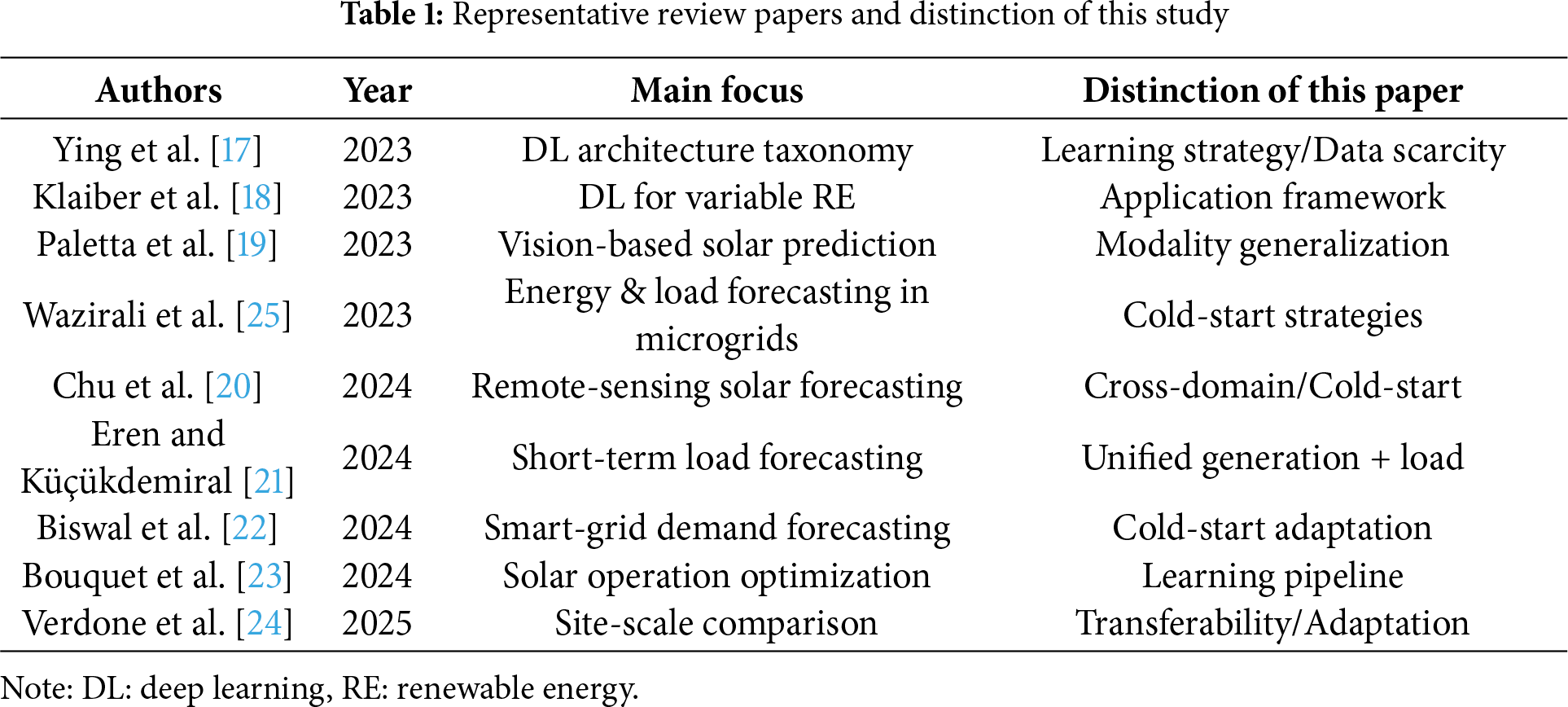
As shown in Table 1, several recent surveys have sought to organize the rapid progress of DL applications in renewable energy forecasting. Ying et al. [17] provided a structural taxonomy of models, and Klaiber and Van Dinther [18] summarized computational trends across variable renewable sources. Domain-focused works such as Paletta et al. [19] and Chu et al. [20] explored vision-based and remote-sensing approaches for solar forecasting, while Eren and Küçükdemiral [21] and Biswal et al. [22] focused on load and demand prediction frameworks. In parallel, Bouquet et al. [23] emphasized operational optimization, and Verdone et al. [24] compared single- and multi-site forecasting performance. Collectively, these studies have contributed substantially to understanding DL architecture and application-specific performance. Yet, most remain confined to descriptive taxonomies—categorizing models or domains—without examining how learning strategies themselves can adapt when data are scarce, incomplete, or imbalanced. This omission leaves a critical methodological gap between architectural innovation and practical deployment.
To bridge this gap, the present review adopts a strategy-centered and cross-domain perspective that treats the cold-start problem as a learning challenge rather than a mere data limitation. By synthesizing insights from meta-learning, transfer adaptation, synthetic data generation, and explainable large language model (LLM)-based forecasting, it establishes a unified analytical framework for adapting DL models under data scarcity. This approach is vital because real-world renewable systems rarely possess abundant, stable data—especially during early-stage deployment—precisely when forecasting accuracy is most needed. Existing reviews have largely overlooked this intersection between data constraints and learning adaptability, which defines the actual boundary of model usability. By connecting fragmented progress—from Wazirali et al. [25] on microgrid forecasting to Bouquet et al. [23] and Verdone et al. [24] on scalability and adaptation—this study advances a cohesive research agenda for robust, scalable, and generalizable cold-start forecasting across renewable energy domains.
This review primarily examines three interrelated domains—solar PV, wind power, and electrical load forecasting—where data scarcity and operational variability make cold-start conditions particularly critical. These sectors capture the most data-challenged and operationally sensitive components of modern power systems. Selected studies on hydropower and carbon-emission prediction are also included to illustrate how learning strategies can extend beyond variable renewables. In contrast, geothermal and bioenergy systems are generally dispatchable and supported by long, stable operational records [26,27], while tidal resources are highly predictable owing to astronomical cycles such as the 18.6-year nodal period [28]. This focus aligns with international classifications that identify solar and wind as variable renewables with the highest operational uncertainty [29,30].
This study makes the following contributions:
• Bridging a critical methodological gap: This review provides the first foundational guide that consolidates fragmented research on cold-start forecasting. By aligning learning strategies with real-world deployment contexts, it helps researchers and practitioners make informed methodological choices and accelerates the operational readiness of renewable forecasting systems under data scarcity.
• Establishing a strategy-oriented synthesis: Beyond architectural taxonomies, this review presents a concise synthesis of key DL paradigms—including TL, meta-learning, ST-GNNs, synthetic data generation, and LLM-assisted explainable artificial intelligence (XAI) [31]—tailored for cold-start forecasting. This synthesis establishes a unified framework for adaptive learning across domains.
• Delivering an evidence-based comparative evaluation: Over 120 peer-reviewed studies are critically analyzed to assess forecasting accuracy, computational cost, generalizability, and implementation feasibility. This comparative approach highlights which strategies perform best under different constraints and provides actionable insights for both research and industrial deployment.
• Defining the forward research agenda: The review identifies persistent research gaps and technical challenges—including interpretability, uncertainty-aware learning, and cross-domain adaptation—and outlines clear directions toward robust, scalable, and transparent cold-start forecasting frameworks for next-generation renewable energy systems.
To help readers make sense of the heterogeneous methods surveyed in this work, Fig. 1 consolidates them into a single, coherent conceptual map. Rather than functioning as a simple summary, the figure illustrates how the three methodological strands—label-efficient learning, spatiotemporal modeling, and generative data augmentation—interact to alleviate the data scarcity inherent in cold-start scenarios. By linking each strand to the relevant sections of the review and showing how these ideas ultimately converge in a reliable, human-centered deployment framework, the figure provides a navigational guide that ties the paper’s theoretical arguments to their practical ramifications.
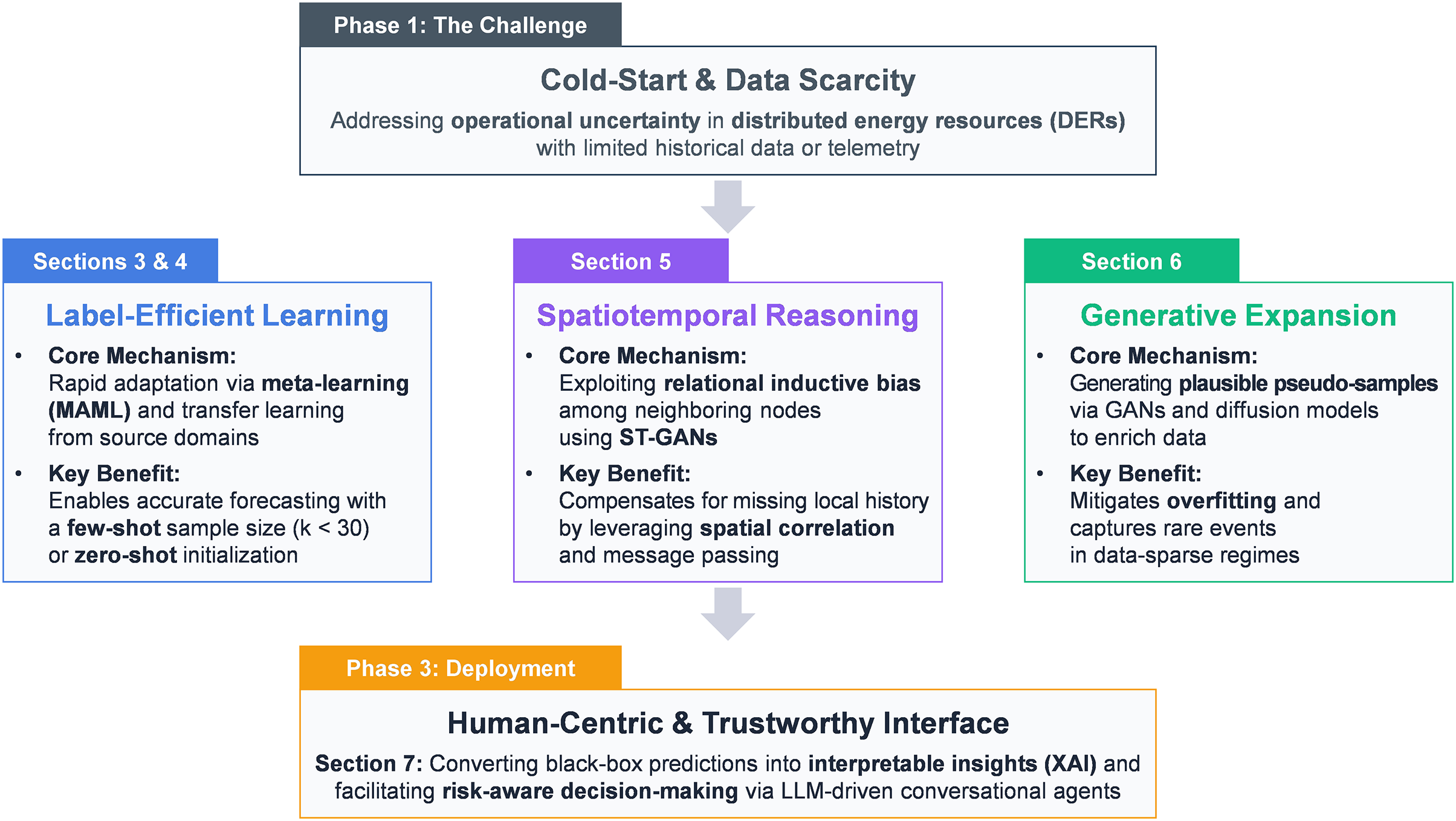
Figure 1: Conceptual framework of the review illustrating the flow of deep learning strategies for cold-start energy forecasting. The diagram highlights the four main contributions analyzed in this paper: (1) Label-efficient learning (meta/transfer learning, Sections 3 and 4) for rapid adaptation; (2) Spatiotemporal modeling (ST-GNNs, Section 5) for leveraging spatial correlations; (3) Generative augmentation (synthetic data, Section 6) for enriching sparse datasets; and (4) Explainable interfaces (XAI/LLMs, Section 7) for operator trust. These components collectively bridge the gap between data scarcity and operational reliability
The rest of this review is structured as follows. Section 2 provides an overview of forecasting models and their cold-start limitations, and Section 3 covers meta-learning for rapid generalization with few examples. Then, Section 4 examines TL for cross-site adaptation, and Section 5 reviews ST-GNNs for spatiotemporal dependency modeling. Next, Section 6 highlights data augmentation as a cold-start solution, and Section 7 discusses LLMs and XAI in relation to transparency and user interaction. Finally, Section 8 outlines open challenges and future work, and Section 9 concludes with practical guidelines for data-scarce forecasting.
2 Forecasting Approaches and Cold-Start Limitations in Deep Learning
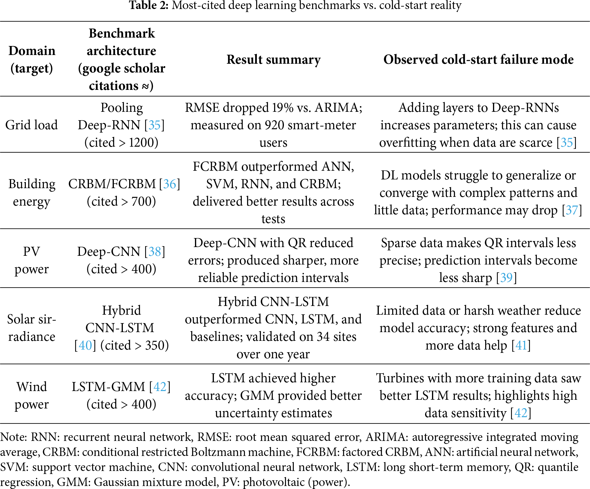
Short-term energy forecasting, ranging from intra-hour to day-ahead projections, is pivotal across all layers of contemporary power systems, encompassing the bulk grid load, building-level demand, PV output, solar irradiance, and wind-farm generation [32]. Although DL can achieve state-of-the-art accuracy in these domains, most prominent studies have relied on months or years of meticulously curated historical data. However, when a newly commissioned asset enters the grid with only a few days of operational history, these models often have critical blind spots. This problem has often been overlooked in the literature. This issue is most pronounced in variable renewables—especially solar PV and wind—because their output shifts quickly with weather changes, unlike the steadier behavior of dispatchable resources [33,34]. Table 2 presents a representative, highly cited DL study of each forecasting domain, highlighting their influence on current practice and examining how its performance degrades under limited historical data conditions.
2.1 Recurrent Neural Architectures under Cold-Start Constraints
The RNN methods, including long short-term memory (LSTM) and gated recurrent units (GRU), were among the first architectures to gain widespread use in energy forecasting [43]. The appeal of these systems stems from their capacity to manage temporal patterns, including the ability to adapt to daily cycles, seasonality, and other temporal correlations that define electricity demand and renewable generation. When trained on extensive datasets encompassing multiple months, these models typically yield highly accurate results [44,45]. However, this success is predicated on the constant availability of substantial, pristine historical data [46].
This success is also predicated on the assumption that months or years of consistent operational data are readily available, which is often not the case in practice. For instance, a newly commissioned solar plant or microgrid node may initiate operations with only a few days of monitoring. In such circumstances, the efficacy of LSTM-based architectures diminishes. These networks require massive datasets to mitigate the risk of overfitting, given their extensive number of trainable parameters, which range from thousands to millions [47]. When confronted with the challenge of training on limited datasets, these models often prioritize memorizing noise over discerning meaningful patterns [48].
In the DrivenData “Power Laws” challenge [49], participants had to predict building energy use with just 1 to 14 days of data for each site. Both organizers and competitors observed that standard LSTM models struggled under these constraints, with DL approaches often failing to generalize when historical data were scarce. This underscores a common cold-start problem: when faced with very short consumption records, LSTMs are prone to overfitting or weak performance. Ahmed et al. [50] showed that PV forecasting with LSTM improves as more historical data become available, while performance drops when data are limited. Their results make it clear that LSTMs struggle to converge and generalize in cold-start or short-history scenarios.
These cases exemplify a more extensive concern: the incongruity between the intricacy of the model and data accessibility during the preliminary implementation phases. Although these architectures remain valuable, their fragility during initialization requires complementary approaches. Section 2.3 presents a comparative synthesis of these limitations across model families.
2.2 Transformer-Based Forecasting in Data-Scarce Environments
Transformer-based models have transformed the landscape of time-series forecasting by capturing distant temporal dependencies that earlier architectures have struggled to represent [51]. Zhou et al. [52] introduced an influential contribution called the informer model, which integrates ProbSparse self-attention with a novel generative decoding mechanism. This design reduces computational complexity to O(LlogL) and delivers consistently strong performance across a range of public energy datasets, including transformer oil temperature and electricity consumption, surpassing LSTM and standard transformer baselines.
However, these models are not immune to the challenges posed by sparse data. Transformers require a considerable volume of data for optimal performance [53]. The mechanisms employed by these systems to identify reliable key-value pairs depend on high token density. The efficacy of this mechanism is compromised in scenarios characterized by scarce input sequences, referred to as cold-start conditions. Although optimized for efficiency, the architecture of the informer model still displays deficiencies when the volume of historical records is inadequate to anchor attention patterns [54].
This limitation becomes problematic in day-ahead forecasting tasks, where the model must relate future weather patterns to energy output with minimal context. In such circumstances, transformer-based architectures often yield uncertainty estimates that are not readily applicable in practice. While these models are technically advanced, they demonstrate fragility when applied to early-stage deployments with sparse data. Section 2.3 further contextualizes this limitation via a comparative analysis.
2.3 Comparative Analysis of Deep Learning Architectures under Cold-Start Constraints
Although individual case studies can explain model behavior under cold-start conditions, a broader comparison across architectural families reveals recurring patterns. Table 3 provides a comparative analysis of two widely adopted model classes: sequence-oriented networks (e.g., LSTM and GRU) and attention-based architectures (e.g., informer). This analysis underscores the primary strengths of the mentioned models in data-rich settings and their failure modes when historical records are scarce.
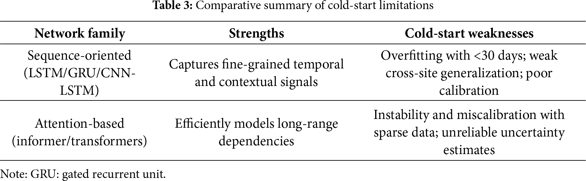
Despite their strong empirical performance on long-horizon benchmarks, these models are fundamentally designed for data abundance. In practice, the early deployment of energy systems often furnishes only limited operational history. Under such conditions, complex architectures tend to overfit, display poor generalization, and produce unreliable uncertainty estimates. These architectures have been broadly incorporated into residential load forecasting and building-energy modeling pipelines [35,36,44,45], while also supporting forecasting in renewable-energy domains such as solar PV and wind generation [38,40,42]. Their extension to long-sequence time-series forecasting [52] reflects their growing methodological reach. Nonetheless, empirical evidence increasingly points to structural weaknesses, including overfitting under sparse historical data, limited spatial transferability across climates, and instability in modeling multi-scale meteorological drivers, that warrant careful examination.
This diagnostic comparison underscores the need for specialized cold-start solutions. Various approaches, including TL, few-shot meta-learning, and physics-informed pretraining, help resolve the mismatch between model complexity and sparse real-world data. To clarify the shift required for next-generation forecasting, Fig. 2 outlines the field’s evolving trajectory. In contrast to the static methodological map in Fig. 1, this diagram places emphasis on how operational workflows diverge between traditional, data-intensive architectures and the cold-start pipelines introduced in this review. It highlights the pivotal movement away from point-based forecasting—effective only when ample historical records exist—toward risk-aware and label-efficient strategies designed to function during the earliest stages of deployment. By presenting this comparison, the roadmap offers a strategic bridge between the limitations of existing models and the adaptive techniques explored in the sections that follow.
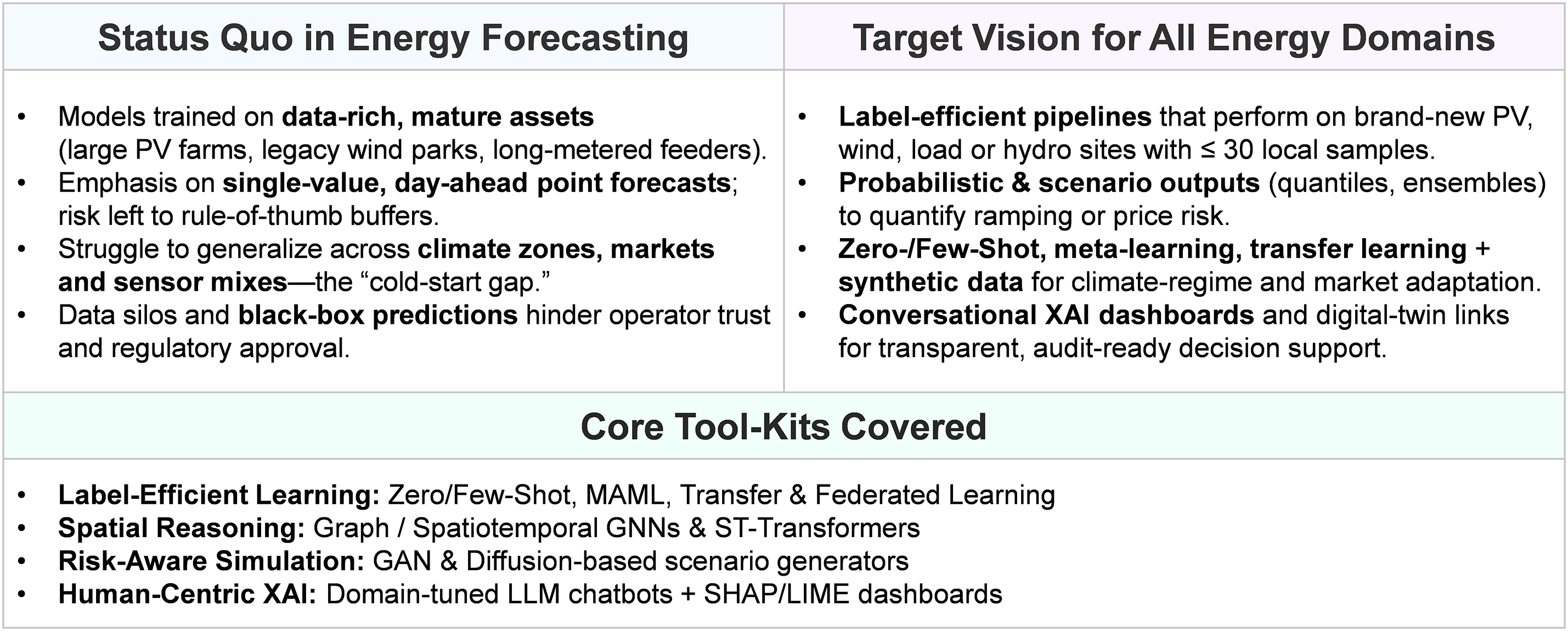
Figure 2: Road map from data-rich forecast models to label-efficient, risk-aware, and explainable pipelines for cold-start energy forecasting across energy domains (photovoltaics, wind, load, etc.). The roadmap is centered on PV and wind—where cold-start conditions are most severe—but the principles can extend to other renewables with appropriate domain considerations (see Section 8)
3 Zero-, Few-Shot, and Meta-Learning Strategies for Cold-Start Forecasting
Although short-term energy variables (e.g., solar irradiance and wind speed) follow certain physical regularities, accurate forecasting still typically relies on extensive historical records [55]. However, these data are often unavailable during the initial deployment of new energy systems [56]. In low-data contexts, conventional DL models commonly underperform due to their high parameter count relative to the limited training input.
Recent work has applied meta-learning techniques that enable models to generalize rapidly by drawing on prior experience from related tasks to address this limitation [13]. Rather than learning from scratch, these methods aim to identify shared structures that can be reused across settings. A representative example is the model-agnostic meta-learning (MAML) pipeline [57]. In this framework, a model is trained on multiple source tasks to obtain a generalized initialization, which is subsequently fine-tuned using only a few samples from the target site [58].
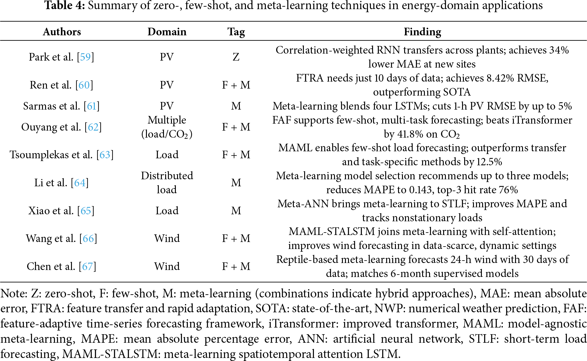
This section outlines the design principles of such approaches and explains why they are well-suited to cold-start forecasting. Moreover, this section synthesizes the findings from recent studies that evaluate meta-learners under limited data conditions. In Table 4, various meta-learning strategies have demonstrated substantial performance gains across energy domains, even when fewer than 50 training examples are available. These results reinforce their potential as a viable solution to the data sparsity challenge in early-stage deployments.
To quantitatively interpret the linguistic structure of recent zero-, few-shot, and meta-learning studies in energy forecasting, a statistical text-mining procedure based on term frequency-inverse document frequency (TF-IDF) weighting was conducted. Each token’s contribution to the corpus was measured as TF-IDF(t, d) = TF(t, d) × log(N/DF(t)), where N denotes the number of reviewed documents and DF(t) the document frequency of term.
Fig. 3 summarizes the 20 most dominant keywords, presenting their total TF-IDF sum, document frequency, and normalized weight. The results show that meta, power, PV, task, and load consistently achieve the highest statistical relevance across the analyzed corpus. These terms correspond to central methodological trends reported in Table 4, where meta-learning and few-shot strategies repeatedly appear as key mechanisms for addressing data sparsity in cold-start forecasting.
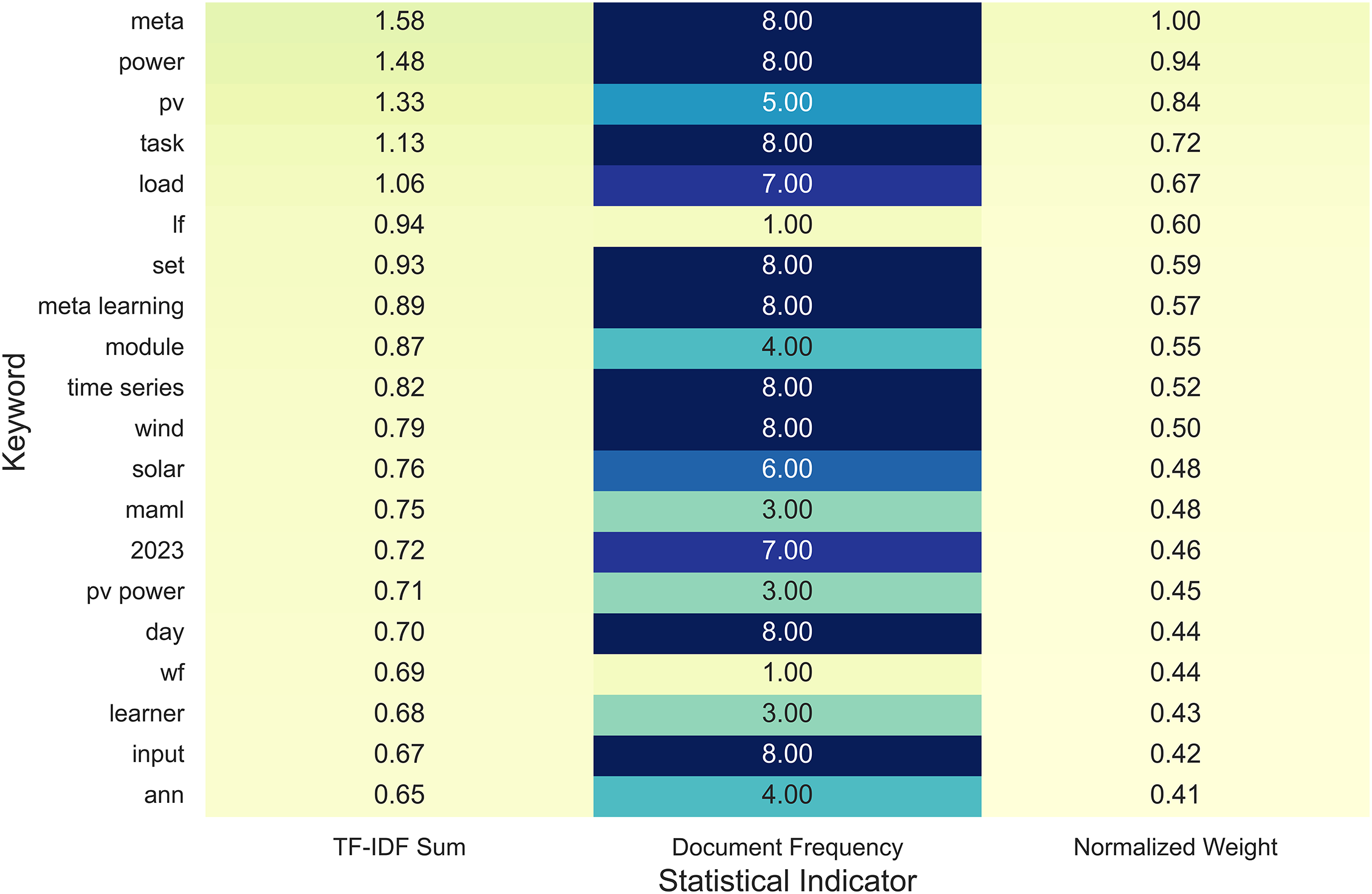
Figure 3: Quantitative summary of dominant keywords in meta-learning literature (TF-IDF analysis)
The quantitative distribution in Fig. 3 thus provides empirical evidence that recent energy-domain literature has converged on meta-learning paradigms such as MAML, feature-adaptive frameworks, and correlation-weighted transfer schemes. By linking statistical keyword dominance with reported physical mechanisms and forecasting outcomes, this analysis reinforces the scientific consistency between textual emphasis and methodological advancement—thereby enhancing the analytical rigor of the study beyond purely descriptive reporting.
To assist readers in identifying conceptual proximity among recent studies, a hierarchical similarity map was constructed using the cosine similarity of TF-IDF representations for each reference document. This analytical approach measures the directional alignment between documents as Sim(A, B) = (A⋅B)/(∥A∥∥B∥), and applies Ward’s hierarchical linkage to cluster studies that share lexical or thematic overlap.
Fig. 4 visualizes this relationship as a dendrogram-integrated heatmap, where closer branches indicate stronger textual coherence and methodological alignment. For instance, studies [59,61] exhibit high cosine similarity (>0.75), reflecting their shared emphasis on meta-learning frameworks for few-shot forecasting. In contrast, works such as [64,67] occupy more distant clusters, indicating distinctive problem formulations or domain focuses (e.g., distributed load vs. wind prediction).
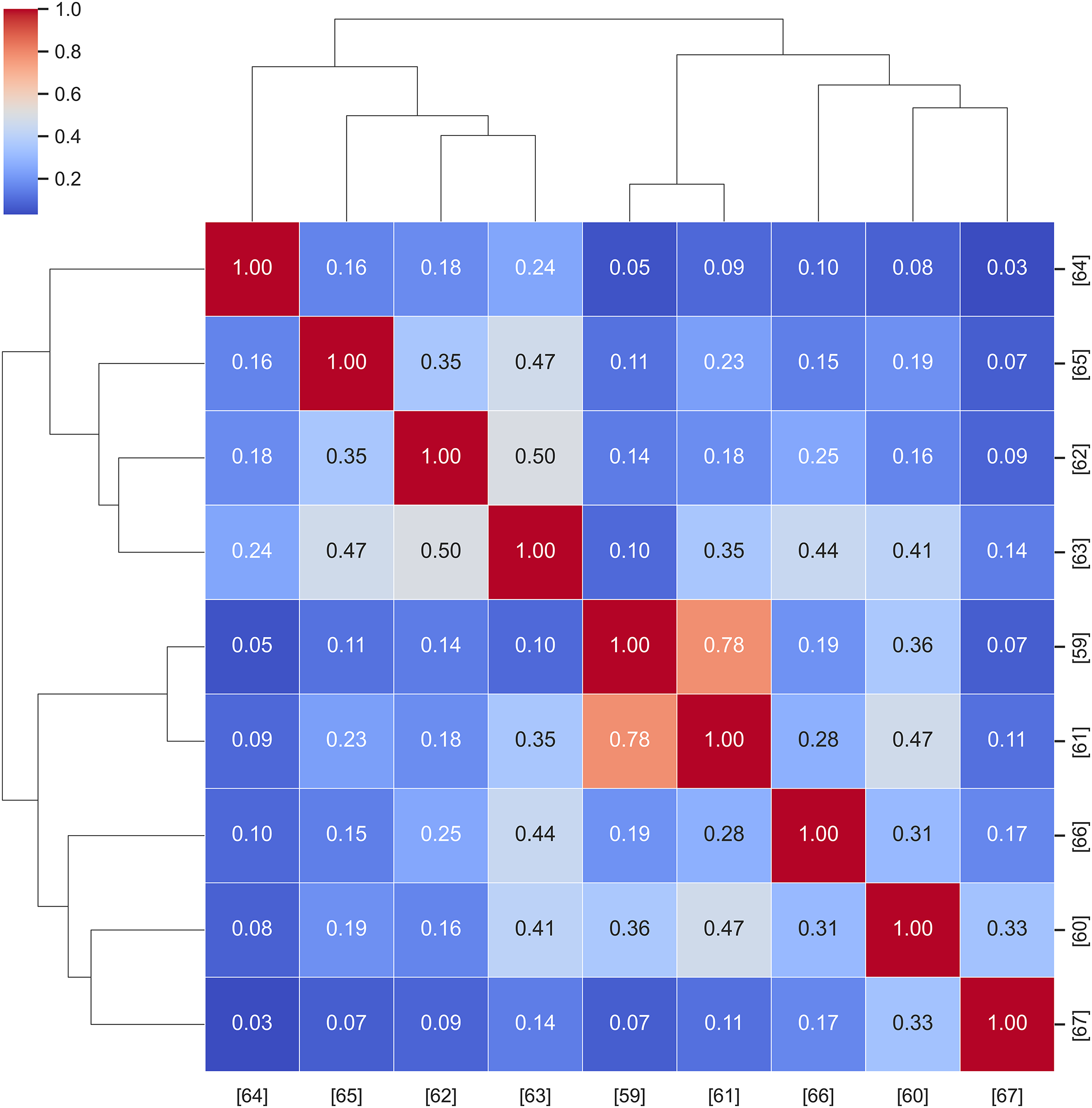
Figure 4: Hierarchical similarity map among meta-learning studies (TF-IDF cosine + Ward linkage)
This hierarchical structure not only validates the internal consistency of the reviewed corpus but also helps readers systematically explore related research directions, enabling targeted comparison among studies with similar methodological orientations. Such interpretive visualization enhances the transparency, reproducibility, and analytical depth of the literature synthesis, demonstrating the robustness of the present study’s quantitative framework.
To provide an interpretable overview of how research themes are distributed across the meta-learning corpus, a keyword landscape was constructed using principal component analysis (PCA) on the cosine similarity matrix of TF-IDF term vectors. This deterministic approach projects high-dimensional keyword representations into an orthogonal two-dimensional plane defined by the leading eigenvectors of the covariance matrix XTX.
Fig. 5 visualizes the resulting semantic topology. Each circle represents a keyword, sized according to its normalized TF-IDF weight and colored by its assigned cluster. The use of cosine-based PCA ensures that the spatial distance between terms directly reflects their lexical and contextual similarity, enabling a quantitative yet intuitive understanding of the thematic structure.
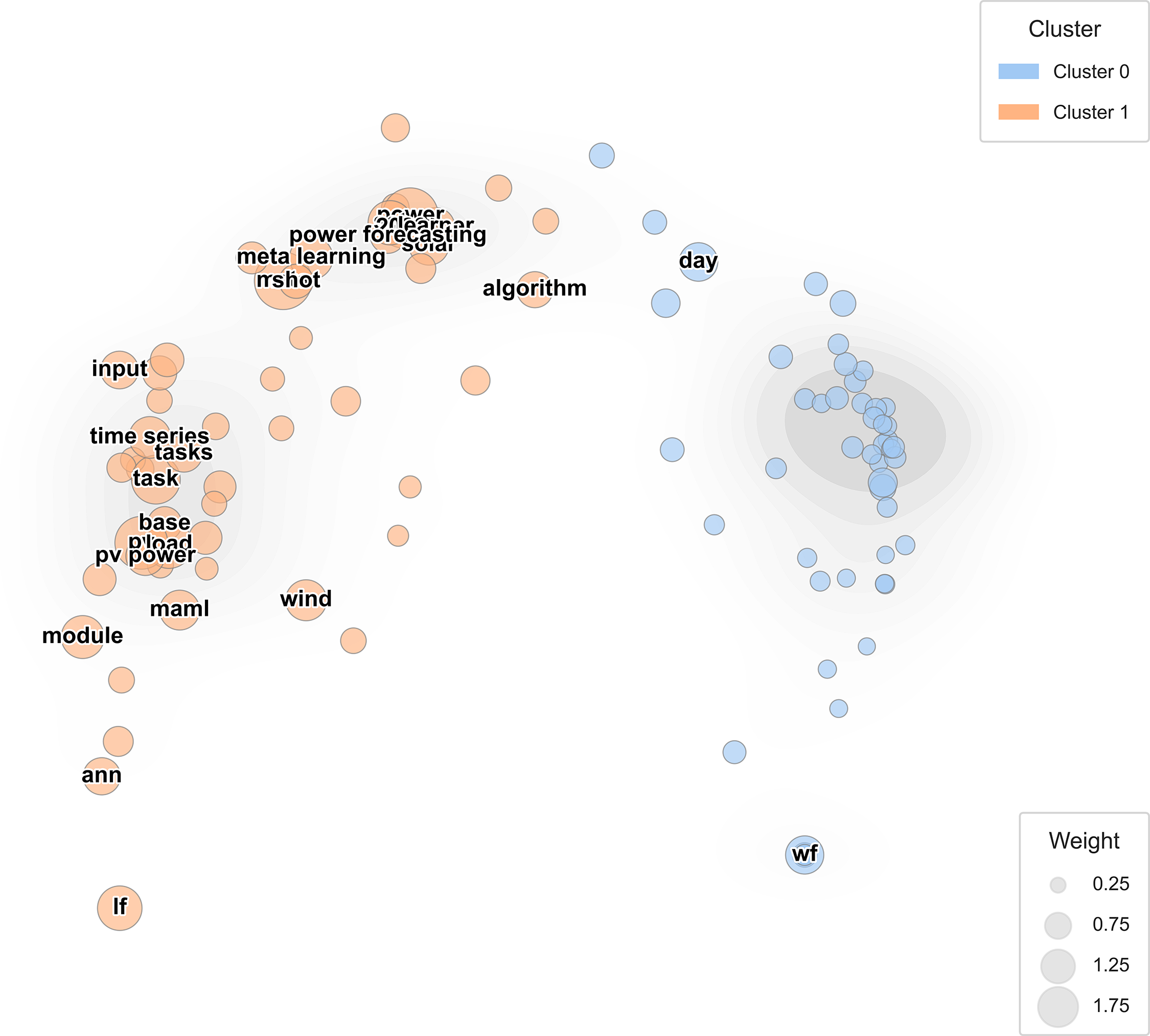
Figure 5: Keyword landscape of meta-learning literature (PCA + cosine similarity)
As illustrated in Fig. 5, the spatial organization of the semantic topology highlights a notable pattern: the close proximity of “MAML” and “PV power” within the high-density subregion (Cluster 1) suggests a concentrated body of work where meta-learning is increasingly applied to solar forecasting challenges. This clustering implies that MAML has evolved from a primarily conceptual technique into a frequently adopted operational tool for managing solar-driven variability, particularly in settings where rapid cross-task adaptation is required.
This visualization helps readers navigate the conceptual landscape of meta-learning studies by identifying clusters of recurring research patterns and highlighting transitions between task-level optimization and domain-level adaptation. Unlike heuristic word maps, this PCA-based analysis is fully reproducible and statistically grounded, thus reinforcing the analytical rigor of the literature synthesis.
3.1 Model-Agnostic Meta-Learning
Energy time series, encompassing the grid load and PV output, are subject to fluctuations influenced by meteorological conditions, policy, and user behavior [68]. However, acquiring new labeled data is often time-consuming. Conventional DL models require retraining from the outset to maintain precision, which is costly and occurs after operations have begun. Meta-learning has emerged as a remedy for the label scarcity and distribution drift that plague operational energy forecasting [69]. Rather than requiring the extensive retraining of a deep network from its fundamental components, a meta-learner first identifies a generic representation. This representation can undergo recalibration in real time with a limited number of new data points. The most prominent instantiation of this concept is MAML, which is compatible with any gradient-based model and fits naturally into the CNN, LSTM/GRU, and transformer toolkits already familiar to energy analysts.
Finn et al. [70] introduced MAML by explicitly optimizing Eqs. (1) and (2) with convolutional classifiers, sinusoid regressors, and policy-gradient agents. Because Eq. (1) uses only one to five examples per task, the tasks could demonstrate state-of-the-art few-shot image classification and markedly faster fine-tuning of reinforcement-learning policies. Crucially, the algorithm is model-agnostic (i.e., any network that admits backpropagation can be integrated into the two-line loop), making the method a standard benchmark for research on rapid adaptation. The algorithmic structure of this approach is visualized in Fig. 6, which explicitly maps the transition from global initialization to task-specific parameters.
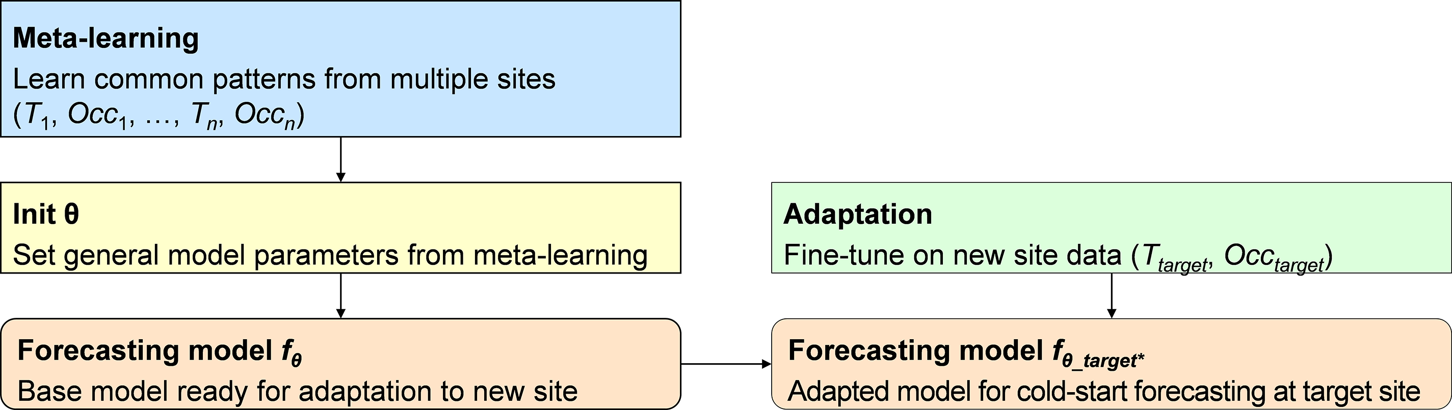
Figure 6: Model-agnostic meta-learning-based cold-start forecasting pipeline. A model is trained on source tasks to learn a general initialization θ, θ yield an adapted forecaster fθ∗target
As illustrated in the figure, the MAML algorithm consists of two alternating optimization steps that cycle between task-specific adaptation and global refinement:
Eq. (1) represents the inner-loop adaptation shown in the diagram, where the global initialization (
Ssekulima et al. [55] employed the same mechanics in short-term electric load forecasting using the meta-artificial neural network (Meta-ANN). A long-horizon base ANN first absorbs multiyear Belgian grid data to capture trends and seasonality. Just before each daily forecast, an error-correction module applies Eq. (1) to the previous day’s residuals, recalibrating the model with only a few fresh observations. Joint training via Eq. (2) allows Meta-ANN to outperform the conventional ANN and statistical baselines consistently, confirming that the fast-adaptation principle of MAML extends smoothly from controlled vision benchmarks to nonstationary energy time-series.
This study demonstrates that the inner/outer-loop paradigm of MAML transfers from vision and reinforcement learning to real-world energy time series, achieving meaningful accuracy increases with minimal daily adaptation. Meta-learning remains effective using only simple, interpretable input (calendar and lagged load) even in low-dimensional settings, supporting zero- or few-shot learning, as real deployments often lack sufficient labeled data per site or day, but demand rapid adaptation from limited recent observations.
Zero-shot forecasting refers to the application of a pretrained model to a new domain without additional fine-tuning or local gradient updates [71]. Rather than retraining, the model relies on patterns learned from previous datasets, assuming that the structural characteristics of the new task are sufficiently represented in the original training space. This method draws inspiration from the behavior of LLMs, which can often respond to novel prompts by generalizing from prior knowledge alone [72]. When structural alignment exists, zero-shot forecasts can yield credible output even without site-specific data.
Crucially, performance tends to degrade gracefully, rather than fail completely, when the target domain differs from the source [73]. The operational logic of the zero-shot procedure is illustrated in detail in Fig. 7 [59]. As depicted, the framework begins by evaluating similarity scores between the target site and a library of reference locations using meta-level descriptors. These similarity measures act as adaptive weights, enabling the model to assemble a target-aware predictor through a selective aggregation of the most relevant source models. By constructing this weighted ensemble, the system can produce actionable forecasts even in the absence of initial on-site telemetry, thereby circumventing the conventional data accumulation period required by standard approaches.
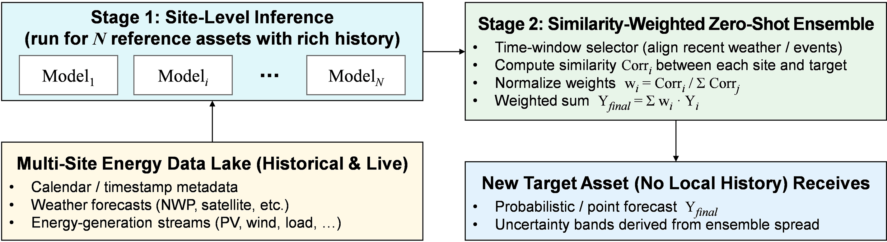
Figure 7: Correlation-weighted zero-shot ensemble for rapid, cold-start energy forecasting
Park et al. [59] illustrated this phenomenon (i.e., zero-shot forecasting) in the energy domain by implementing a correlation-weighted RNN trained on eight PV sites for a ninth site, without local data use. Without target samples, the mean absolute error (MAE) of the model was reduced by 34% compared to the baseline. In a broader context, Oreshkin et al. [74] introduced a residual-meta architecture based on N-BEATS (short for Neural Basis Expansion Analysis for interpretable Time-Series forecasting), trained across a collection of diverse univariate time-series (e.g., electricity demand and commodity indices) and demonstrated that, even in zero-shot mode, their framework matched or outperformed classical methods (e.g., ARIMA and exponential smoothing) on many of these datasets.
Such zero-shot capabilities are relevant in operational settings where data may be sparse or temporarily unavailable. This outcome underscores the efficacy of structured, multisite pretraining. For instance, during natural disasters that disrupt supervisory control and data acquisition (SCADA) connectivity, a pretrained model can be rapidly deployed to maintain forecast continuity until local telemetry is restored [75]. In scenarios where even minimal local data collection is feasible, few-shot adaptation offers a compelling compromise, retaining most of the efficiency of zero-shot transfer while significantly increasing accuracy with just a few target-specific observations.
Few-shot forecasting is the process of applying a model that has been exposed to a limited number of labeled instances from the target domain [76]. In most cases, the number of labeled instances is less than 30, and the model uses these instances to perform a form of lightweight adaptation, often updating only a subset of parameters. Mathematically, this process can be interpreted as an empirical Bayes update, where the pretrained model provides a strong prior and a few steps of stochastic gradient descent refine the posterior toward the target distribution [77].
A substantial body of recent research has validated the efficacy of this approach. Ren et al. [60] proposed FTRA (short for Feature Transfer and Rapid Adaptation), a hybrid of TL and Reptile meta-learning, which achieved a maximum reduction of up to 19% in MAE with as few as 10 days of training data in solar power forecasting. Ouyang et al. [62] developed a feature-adaptive framework (FAF) with a modular architecture that disentangles global and local features via a rank-based adaptation layer, yielding a 42% generalization gain across five public datasets, including electricity, carbon emissions, and traffic flows. Tsoumplekas et al. [63] introduced a MAML-GRU framework that enhanced forecasting accuracy by 12.5% on 96 residential load time-series and proposed a novel evaluation metric tailored to the demand-side variability.
From an engineering perspective, few-shot methods are preferred in settings with microgrids or behind-the-meter devices capable of uploading limited daily data [78]. For example, a 10-day period of hourly measurements results in 240 labeled rows, which is sufficient for collection during a single site visit. This measurement volume is sufficient for a meta-trained model to reduce the error by nearly half compared to zero-shot deployment. Hence, few-shot learning offers a pragmatic intermediate solution by maintaining the plug-and-play nature of zero-shot models while achieving substantially higher accuracy when a modest amount of local supervision is accessible.
3.4 Advanced Meta-Learning Frameworks
Meta-learning has advanced beyond parameter initialization to richer architectures that explicitly model the structure of temporal forecasting tasks. A notable example is FAF, which separates knowledge into two components: a generalized module capturing global patterns shared across tasks and a task-specific module tailored to local characteristics [62]. During adaptation, a lightweight ranker selectively activates the most relevant functional regions, allowing the model to integrate both generalized and task-specific knowledge. FAF achieved substantial accuracy gains across diverse datasets—including electricity, CO2, and traffic—outperforming the best baseline (iTransformer) by up to 41.8% on CO2 data, underscoring its effectiveness for few-shot, multi-task forecasting.
A different approach treats meta-learning as an automated model selection rather than as a parameter adaptation. Li et al. [64] introduced a meta-learning-based model selection framework that recommends up to three optimal load forecasting models per task using input series summary features. This automated approach streamlines deployment and reduces average MAPE from 0.188 to 0.143, making it highly practical for real-world applications with diverse forecasting needs.
Another innovation lies in spatially aware meta-learning. Wang et al. [66] combined a self-attention–enhanced spatiotemporal LSTM with MAML, enabling efficient adaptation to new wind farm conditions with minimal training data. Their framework outperformed baselines on both onshore and offshore wind datasets, demonstrating significant gains in forecasting accuracy and robustness, particularly under data-scarce conditions.
Together, these frameworks reveal how meta-learning can be extended beyond initialization to architecture-level design, model selection, and spatial reasoning. In practice, these frameworks indicate a hybrid deployment strategy: begin with zero-shot forecasting when no target data are available, adopt few-shot updates as small batches accumulate, and shift to full retraining once sufficient historical data and computational resources permit it [79]. This layered approach balances accuracy, responsiveness, and operational constraints in real-world forecasting systems.
4 Transfer Learning in Cold-Start Forecasting
Real-world energy forecasting projects often begin in a data-poor regime. New sites may have no or only a few days of telemetry. In such cold-start settings, full meta-training across dozens of related tasks, as required by MAML, is rarely practical. However, TL offers a compelling alternative: it applies a forecasting model pretrained on a single, well-instrumented source domain (e.g., a decade of SCADA data from a utility-scale PV site) and repurposes it for new targets via simple strategies (e.g., weight freezing, gradual fine-tuning, or inserting lightweight adapters) [14]. Thus, TL provides a low-barrier path to meaningful accuracy, even when labeled target data are extremely limited.
Table 5 contrasts the two paradigms across operational axes (e.g., data requirements, computational demands, and update flexibility) to clarify how TL differs from meta-learning in real-world deployments [80]. While MAML excels when task diversity is available and adaptation speed is critical, TL minimizes complexity by working with a single source dataset, avoiding inner-loop gradient calculations, and requiring minimal hyperparameter tuning. Fig. 8 maps the trade-offs between TL and MAML by situating both methods along the axes of data availability and computational burden [81]. The visualization makes it clear that MAML sits in the high-adaptability region, reflecting its strength in rapidly generalizing across heterogeneous tasks, yet this advantage comes with considerable computational expense. TL, by contrast, occupies a more resource-efficient region of the diagram, making it a practical choice when computational budgets are tight—even when only a modest number of training samples are available. This contrast establishes a straightforward decision boundary for practitioners weighing flexibility against efficiency in cold-start forecasting settings.
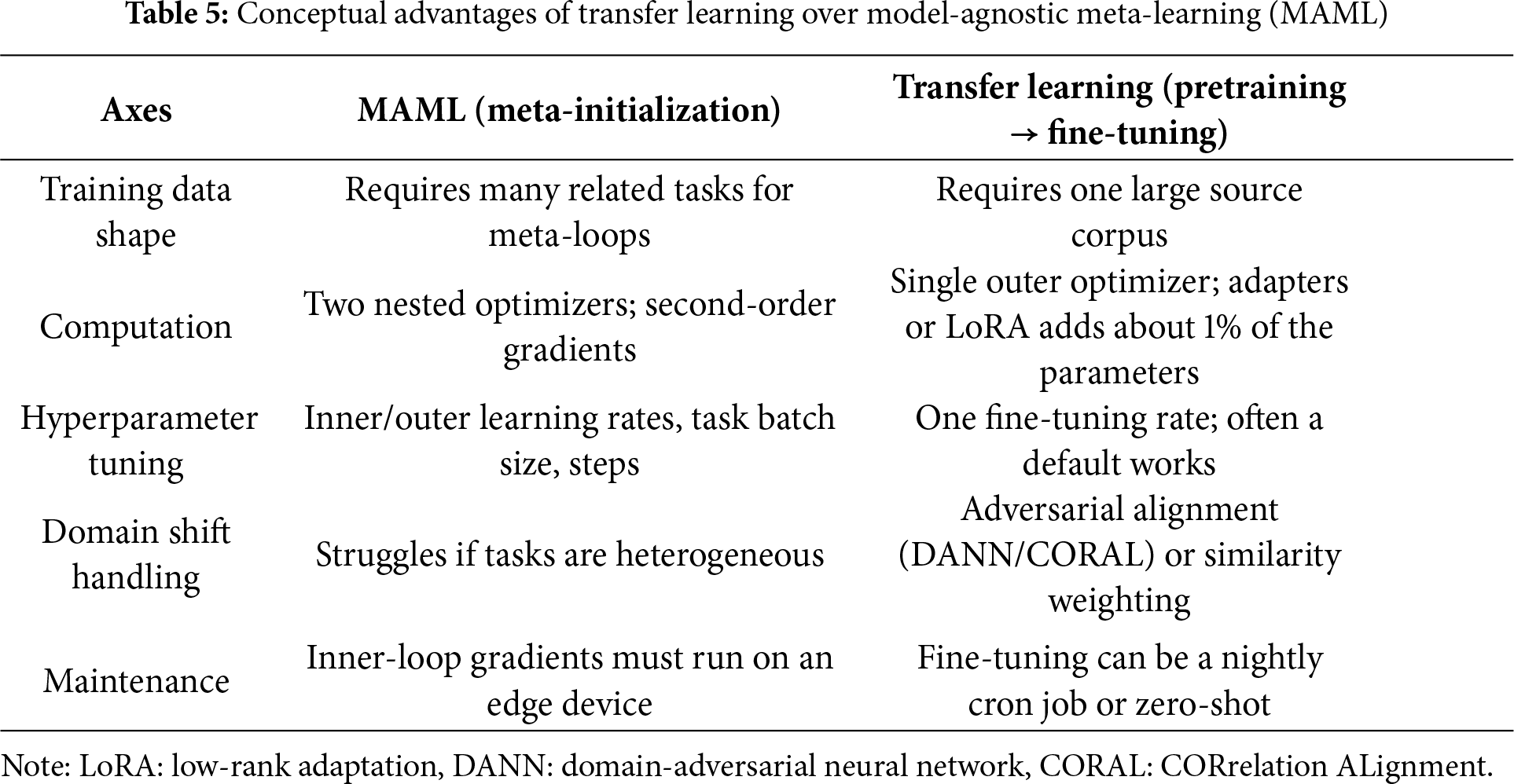
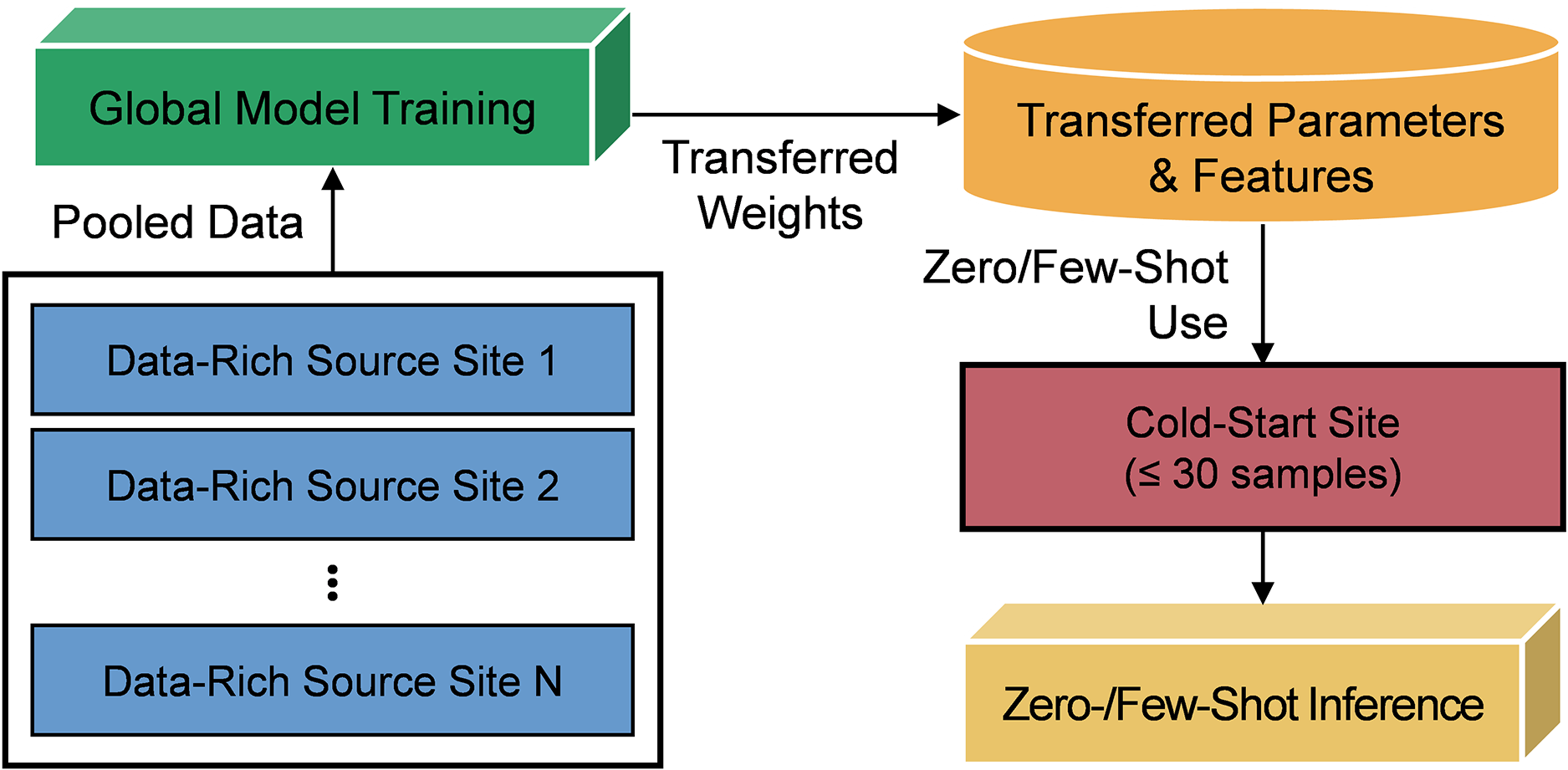
Figure 8: Operational tradeoffs between transfer learning and model-agnostic meta-learning in cold-start energy forecasting
4.1 Mathematical Formulation of Fine-Tuning
To formalize the mechanics of TL, we define the standard fine-tuning step commonly employed in cold-start energy forecasting scenarios. In Eq. (3), a model pretrained on a source domain is updated via a single gradient descent step on the target-site loss:
In this formulation,
This simplicity is advantageous in energy forecasting, where computational constraints often preclude complex meta-learning pipelines. Fine-tuning can be performed by fully updating all weights, partially unfreezing selected layers, or inserting lightweight modules, including adapters or low-rank adaptation (LoRA) [82]. Because the procedure is efficient and scalable, it enables routine on-device updates as new measurements arrive, making it suitable for incremental personalization in grid operations, building-control systems, or remote energy assets.
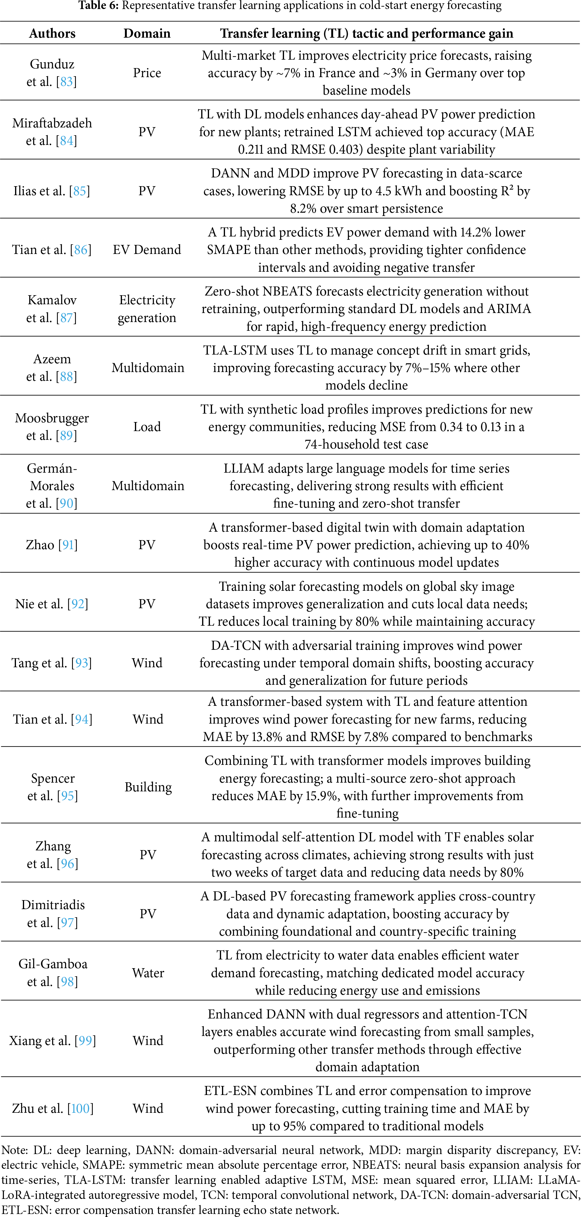
4.2 Representative Case Studies
To ground the conceptual differences highlighted in Table 6 with practical evidence, we present recent studies that apply TL across diverse energy forecasting domains. These case studies demonstrate how TL techniques, from classic fine-tuning to advanced domain adaptation, yield tangible performance gains under real-world constraints.
To connect the conceptual overview in Table 6 with practical linguistic evidence, Fig. 9 illustrates the distribution of high-frequency terms that characterize recent TL studies in energy forecasting. This figure serves as a complementary perspective, showing how researchers across different domains—such as PV, wind, load, and water forecasting—tend to share a common technical vocabulary when applying TL in data-scarce or cold-start conditions.
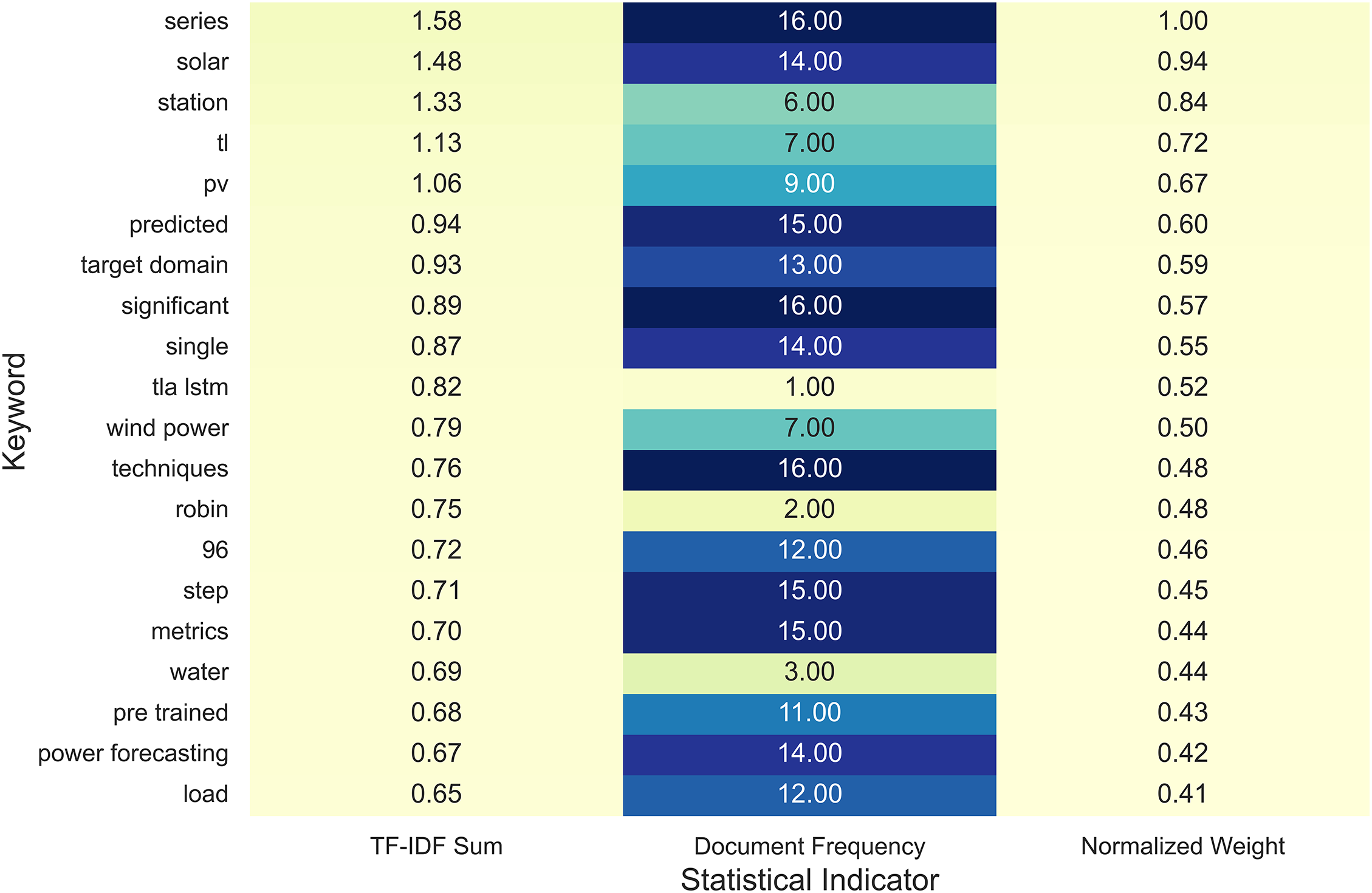
Figure 9: Representative keyword distribution in transfer learning-based energy forecasting studies
The most salient keywords, including series, solar, station, and predicted, emphasize TL’s focus on structured time-series modeling and site-level forecasting. In addition, words like domain, adaptation, and fine-tuning frequently appear, suggesting that modern TL research increasingly targets domain shift mitigation, temporal robustness, and lightweight model reuse rather than simple parameter transfer. Such trends echo the findings in Table 6, where TL has been successfully employed across a wide range of energy applications—from photovoltaic and wind prediction to water demand and building load forecasting—each achieving measurable accuracy gains under constrained data environments.
Taken together, the linguistic distribution in Fig. 9 highlights a clear shift toward transferable, resource-efficient modeling practices. By linking language usage to observed methodological outcomes, this analysis underscores TL’s growing relevance as a pragmatic approach for real-world energy forecasting, offering fast adaptability and reliable performance without excessive retraining.
To further interpret the shared structure among recent TL studies, Fig. 10 visualizes their pairwise similarity using a hierarchical clustering approach based on cosine distance and Ward linkage. This analysis provides a document-level perspective, grouping publications that exhibit comparable linguistic and methodological patterns derived from their full-text content.
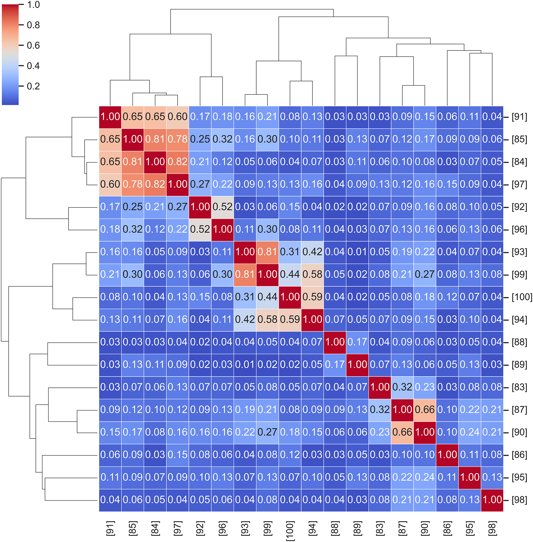
Figure 10: Hierarchical similarity map among transfer learning studies
As illustrated, several clusters emerge with clear topical coherence. For example, studies [84,85,91] form a tight cluster, reflecting their focus on PV power forecasting with domain adaptation and digital-twin frameworks. Similarly, [93,94,99,100] align under wind forecasting applications, where adversarial or temporal adaptation techniques (e.g., DA-TCN, attention-based transfer) dominate. In contrast, papers such as [94,97] display moderate linkage to both wind and PV groups, suggesting hybrid or cross-domain architectures that integrate features from multiple forecasting contexts.
This hierarchical organization quantitatively reinforces the narrative outlined in Table 6—showing that TL studies, despite their diversity of datasets and architectures, tend to converge around a few dominant methodological axes: domain adaptation, temporal generalization, and cross-modal transferability. By mapping textual coherence to research themes, the figure helps readers identify conceptually related works and navigate the literature more effectively. It also demonstrates that the reviewed corpus forms a consistent and interconnected body of research rather than a set of isolated case studies.
To provide a more intuitive view of the conceptual space formed by recent TL studies, Fig. 11 projects the major keywords into a two-dimensional landscape using PCA combined with cosine similarity. This visualization reveals how methodological and application-level terms co-locate, indicating shared thematic structures within the reviewed literature.
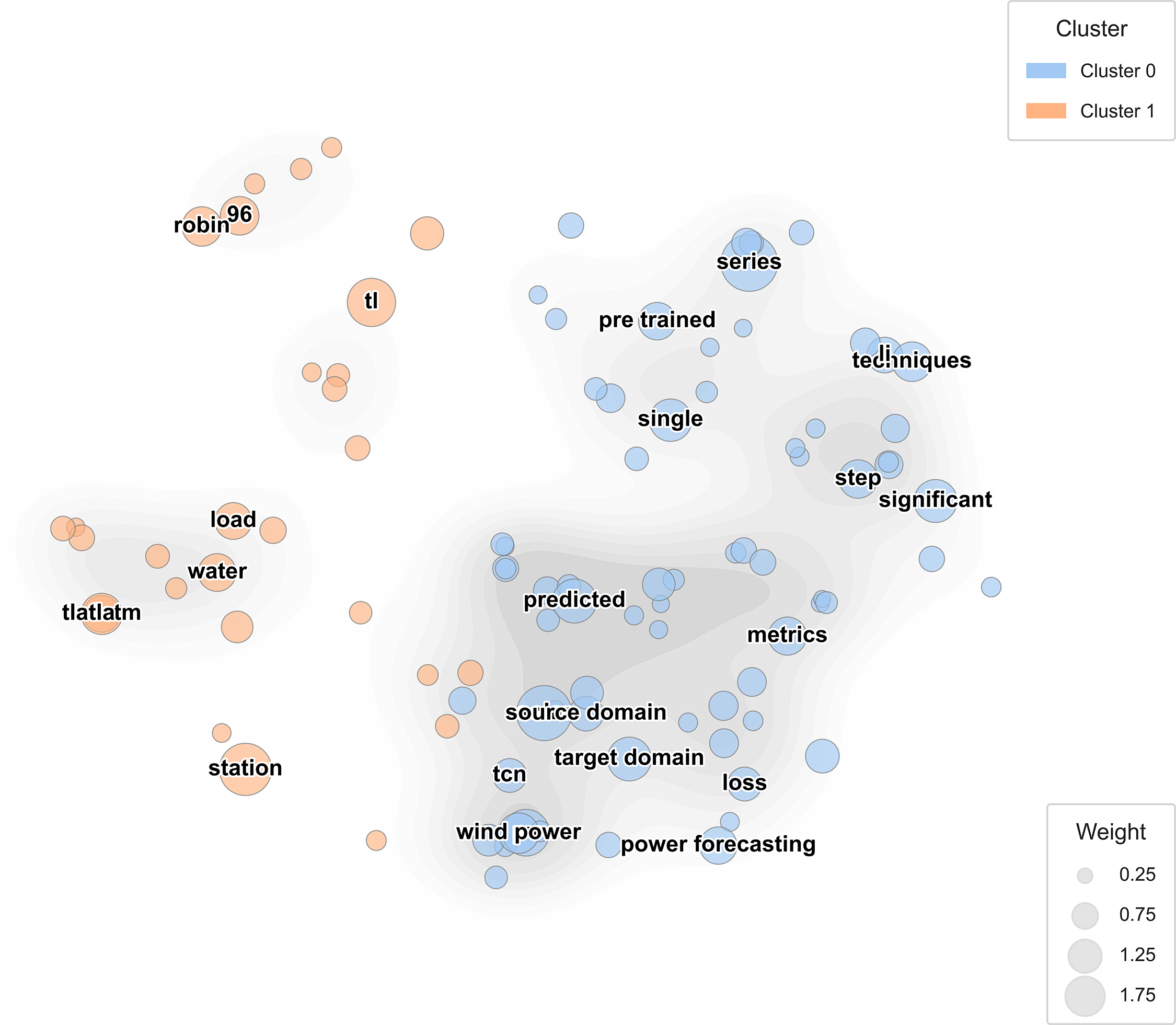
Figure 11: Keyword landscape of transfer learning studies in energy forecasting
The figure separates two broad clusters. The right-hand group (Cluster 0) centers on series, techniques, metrics, and power forecasting, capturing the statistical and procedural language typical of TL implementations for predictive modeling. In contrast, the left-hand group (Cluster 1) gathers around TL, TLA-LSTM, load, water, and station, reflecting studies emphasizing domain adaptation, resource management, and cross-modal transfer between heterogeneous data sources. Intermediate regions link target domain, source domain, and pre-trained—key bridging terms that represent how TL frameworks translate knowledge from one operational setting to another.
By combining linguistic frequency with geometric proximity, Fig. 11 complements the hierarchical patterns shown in Fig. 10. It illustrates how TL research forms a continuous semantic field rather than isolated topical fragments, demonstrating strong internal consistency across applications and methodologies. Such an integrated representation assists readers in recognizing conceptual neighborhoods, helping identify which approaches share transferable principles and which remain domain-specific.
In PV forecasting, Zhang et al. [96] showed that effective weight transfer enables PV forecasting models to adapt from stable to highly variable regions such as Nottingham, UK. Transfer learning significantly cuts training time and data needs while maintaining high accuracy, highlighting its value for robust solar forecasting across diverse climates.
In wind energy, Tang et al. [93] tackled temporal domain shifts in wind power forecasting by combining adversarial training with a temporal convolutional network (DA-TCN). Their approach, which splits training data into temporal domains and jointly optimizes for forecasting and domain discrimination, achieved robust generalization and outperformed benchmarks on real turbine data, showing superior accuracy and stability under changing temporal distributions.
Zhu et al. [100] proposed the error compensation transfer learning echo state network (ETL-ESN) model, which combines error compensation with transfer learning to improve wind power prediction. On the Spatial Dynamic Wind Power Forecasting (SDWPF) dataset, ETL-ESN reduced MAE by up to 98% vs. LSTM and other benchmarks and consistently achieved lower RMSE, demonstrating strong adaptability and reliability for large-scale wind farms.
Across other domains, TL continues to prove versatile. Studies on energy efficiency prediction in petrochemical processes have applied partial layer freezing to balance accuracy and training speed [101]. Digital twin-based transformers can learn domain-invariant features for PV [91], and energy-aware pruning in water metering tasks achieves substantial computational savings without loss of accuracy [98]. Even in zero-shot scenarios (e.g., N-BEATS forecasting of electricity prices with no target data), TL-based initializations deliver competitive MAPE values [87]. Collectively, these cases underscore the adaptability of TL across modalities, time scales, and sensor resolutions. Whether minimizing training costs, accelerating inference, or bridging domain shifts, TL provides a consistent performance benefit, especially in cold-start and resource-constrained environments [102].
4.3 When and Why Transfer Learning Excels
Although meta-learning frameworks (e.g., MAML) provide elegant solutions for fast adaptation, they may not consistently align with the constraints of real-world energy systems [69]. Scenarios involving sparse labels, limited computational budgets, or nonstationary environments often favor TL due to its operational simplicity and adaptability, as TL handles asymmetric data availability more naturally [103]. When only a single rich source corpus is available (e.g., a national SCADA archive), TL can apply it directly, whereas MAML may struggle to generalize with insufficient task diversity. In domains where broad environmental shifts (e.g., seasonal climate changes) are more significant than per-site idiosyncrasies, TL enables explicit distribution alignment via adversarial or similarity-based methods, bypassing the assumption of shared task support that is often embedded in meta-learning [104].
Moreover, TL is well-suited for edge deployment because it requires only a single forward-backward pass per update [105]. Parameter-efficient techniques (e.g., LoRA or adapter modules) can be added with minimal overhead, typically less than 1% of the original parameter count. This lightweight nature contrasts with the memory and computational demands of MAML, which must retain inner- and outer-loop gradients and often requires second-order optimization. Moreover, TL simplifies model maintenance. Fine-tuning can be scheduled as a routine task using cron jobs, without the need for specialized task construction or nested learning rate tuning.
Recent meta-learning approaches for few-shot fault diagnosis highlight this trade-off between adaptability and efficiency. For instance, Zhang et al. [106] proposed an MAML framework for few-shot bearing fault diagnosis, achieving up to 25% higher accuracy than Siamese-network benchmarks and demonstrating strong generalization to new and real faults. Similarly, Zheng et al. [107] developed an improved meta-relation network (IMRN) that leverages multiscale feature encoding and relation-based metric learning; tested on three public datasets, IMRN outperformed other few-shot methods, offering robust and adaptable fault classification with limited data.
The TL method continues to evolve in tandem with broader trends in DL, offering exciting opportunities for the energy domain. One emerging direction is applying foundation models for time series, where large-scale self-supervised pretraining across multiple domains is followed by lightweight task-specific adaptation. For instance, the LLaMA-LoRA–integrated autoregressive model (LLIAM) [90] showed that foundation models pretrained on diverse data can be efficiently adapted for time-series forecasting using lightweight methods such as LoRA. This approach achieves high accuracy and strong generalization with minimal tuning, underscoring the potential of large-scale pretraining followed by efficient adaptation for energy forecasting tasks.
Cross-modal transfer is another promising method. For example, Nie et al. [92] demonstrated that pretraining solar forecasting models on large, multi-location sky image datasets and fine-tuning with limited local data enables robust irradiance prediction, even with 80% less local data than conventional methods. Likewise, Moosbrugger et al. [89] found that transferring from synthetic to real load profiles in energy communities can substantially reduce prediction error (lowering MSE from 0.34 to 0.13), enabling accurate forecasts despite scarce real data. These findings underscore the value of leveraging information across modalities or domains to improve forecasting accuracy and data efficiency.
The TL method prioritizes practicality over complexity, avoiding nested optimization loops in favor of a single, scalable pipeline. This method requires fewer hyperparameters, fits on smaller devices, and begins generating useful forecasts from Day 1. When task diversity is scarce but unlabeled or synthetic data are abundant, TL often outperforms meta-learning in accuracy and deployment speed. The following layered strategy is recommended:
• Begin with zero-shot TL at system commissioning, using a pretrained backbone;
• Begin few-shot fine-tuning after accumulating a week of local data;
• Transition to meta-learning or full retraining once seasonal shifts or operational scaling justify a deeper adaptation.
This hybrid pipeline balances accuracy, speed, and feasibility, providing a robust framework for real-world energy forecasting under evolving data conditions.
5 Graph-Based Spatiotemporal Learning for Cold-Start Forecasting
Many energy infrastructures (from wind farms to power distribution grids) naturally form spatially structured networks [108]. In such systems, the behavior of one node (e.g., a turbine or smart meter) is often shaped by its neighbors, reflecting physical couplings or shared environmental influences. Cold-start forecasting in this context presents a dual challenge: local data are sparse and the topological context may be incomplete or rapidly evolving [11,109]. Recent advances in graph-based spatiotemporal DL address this challenge by integrating two powerful priors: (1) graph topology that captures how entities interact across space and (2) temporal dynamics learned via temporal convolutional networks (TCNs), LSTM networks, or transformers. Together, these models (typically instantiated as ST-GNNs) embed structured domain knowledge directly into the architecture, enabling strong generalization even with minimal local training data [15].
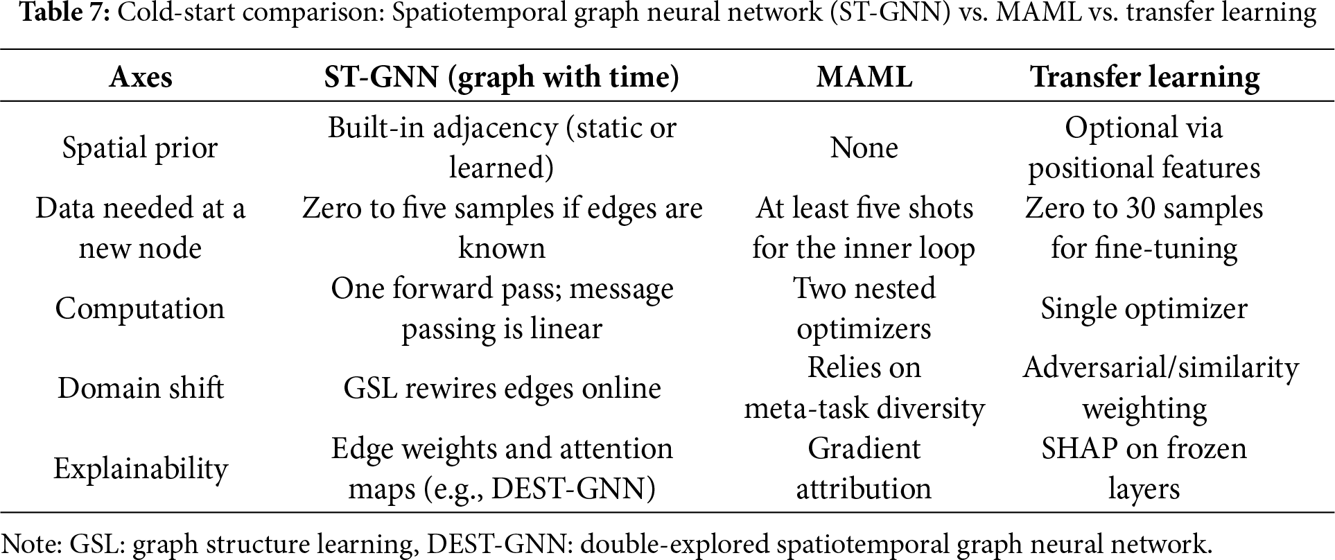
This framework offers two benefits under cold-start conditions. First, it offers relational inductive bias: by encoding who influences whom, the model avoids relearning basic correlations at every site [110]. Second, it offers edge learning modules: dynamic graph-structure learning (GSL) techniques can infer or revise connectivity patterns in real time, easing deployment in sensor-rich or rapidly changing environments [111]. Before addressing representative studies, we contrast the inductive nature of ST-GNNs with the adaptive mechanisms of MAML and TL, as introduced in the previous sections. In contrast to MAML and TL, which focus on optimizing initialization or parameter reuse, ST-GNNs derive generalization directly from the graph-aware architecture [112]. This section conceptually contrasts these approaches, and Table 7 summarizes their cold-start capabilities, focusing on spatial priors, computational efficiency, and adaptability to unseen nodes.
5.1 Spatiotemporal Propagation: Equation and Application
The ST-GNN is a class of models designed to capture spatial dependencies jointly between entities (e.g., PV sites, wind turbines, or distribution feeders) and temporal dynamics in their measurements [113]. By encoding the network topology and time-series history, ST-GNNs provide a rich inductive prior that is suitable for cold-start energy forecasting [114]. With little or no local data, forecasts remain feasible by drawing on information from neighboring nodes. In practice, the input to an ST-GNN comprises a feature matrix Xt for each time step t (e.g., lagged load, irradiance, and calendar features), paired with a graph structure A that describes the inter-node relationships [115]. The output is typically a multivariate forecast vector (e.g., load or generation for the next 1 to 24 h) for each node. Crucially, even if one node has no history, it can still participate in the prediction process via message passing from its neighbors.
A standard layer in these models integrates spatial and temporal components. Many architectures apply a TCN over past measurements to extract local trends and combine this with graph-based aggregation across nodes [115,116]. This layered operation is expressed in Eq. (4):
where
The first term in Eq. (4),
5.2 Representative Spatiotemporal Graph Neural Network Case Studies
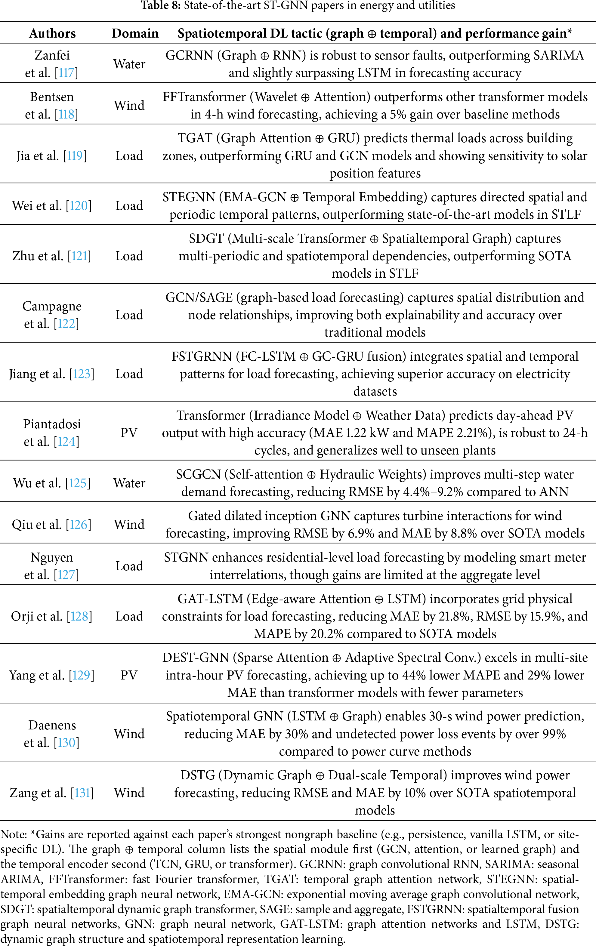
The studies summarized in Table 8 describe recent advances that integrate graph-based relational priors with deep temporal encoders to improve cold-start forecasting across domains, including PV generation, wind power, grid load, and urban water demand. Each model applies spatial relationships derived from physical proximity, electrical topology, or data-driven edge inference to enable predictive reasoning across nodes, even when local labels are sparse or unavailable. These architectures exemplify the potential of spatiotemporal graph learning to generalize in low-data regimes by embedding the structural context directly into the model design.
To highlight emerging trends in graph-based spatiotemporal learning for cold-start forecasting, Fig. 12 presents a statistical summary of the twenty most dominant keywords identified from recent literature. The results reveal how research priorities have shifted from purely temporal architectures toward graph-aware models that encode spatial structure and relational dynamics.
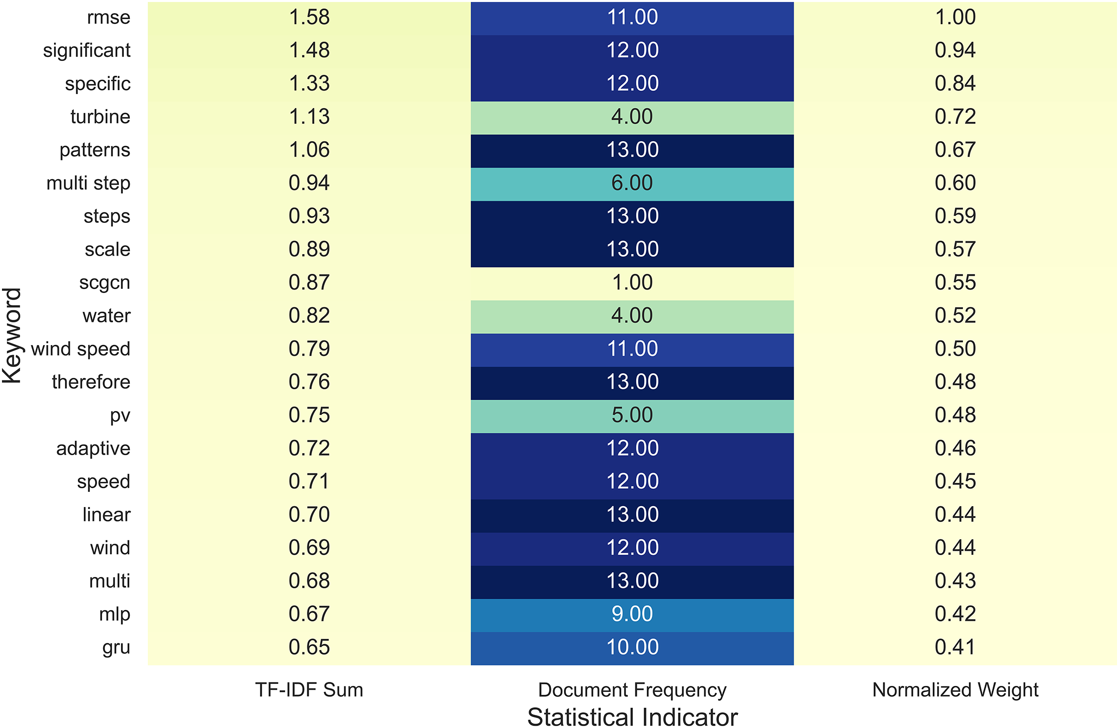
Figure 12: Quantitative summary of dominant keywords in graph-based spatiotemporal learning for cold-start forecasting
Among the leading terms, RMSE, significant, and specific exhibit the highest normalized weights, indicating the community’s increasing focus on quantitative error minimization and statistically interpretable performance metrics. Meanwhile, patterns, multi-step, and scale frequently appear in studies that model hierarchical temporal sequences within spatially coupled sensor networks, suggesting that multi-horizon prediction remains central to ST-GNN design. Notably, SCGCN, wind speed, and PV appear alongside adaptive and linear, signifying the convergence of graph convolution, temporal adaptation, and energy-domain specialization within a unified spatiotemporal framework.
This distribution supports the conceptual contrast outlined in Table 7—showing that, unlike meta- or transfer learning approaches that rely on parameter reuse, graph-based models derive generalization directly from encoded topology and message passing. The quantitative evidence in Fig. 12 thus substantiates the dual inductive bias of modern ST-GNNs: (1) relational coupling among spatial entities and (2) temporal pattern extraction across dynamic contexts. Together, these properties explain why graph-based architectures achieve superior adaptability in data-scarce or rapidly evolving energy systems.
To examine how recent graph-based spatiotemporal forecasting studies relate to one another conceptually, Fig. 13 presents a hierarchical similarity map derived from the cosine similarity of their TF-IDF representations. This analysis quantifies the directional alignment among papers by comparing the linguistic composition of each study, with darker red blocks indicating higher textual coherence and methodological overlap.
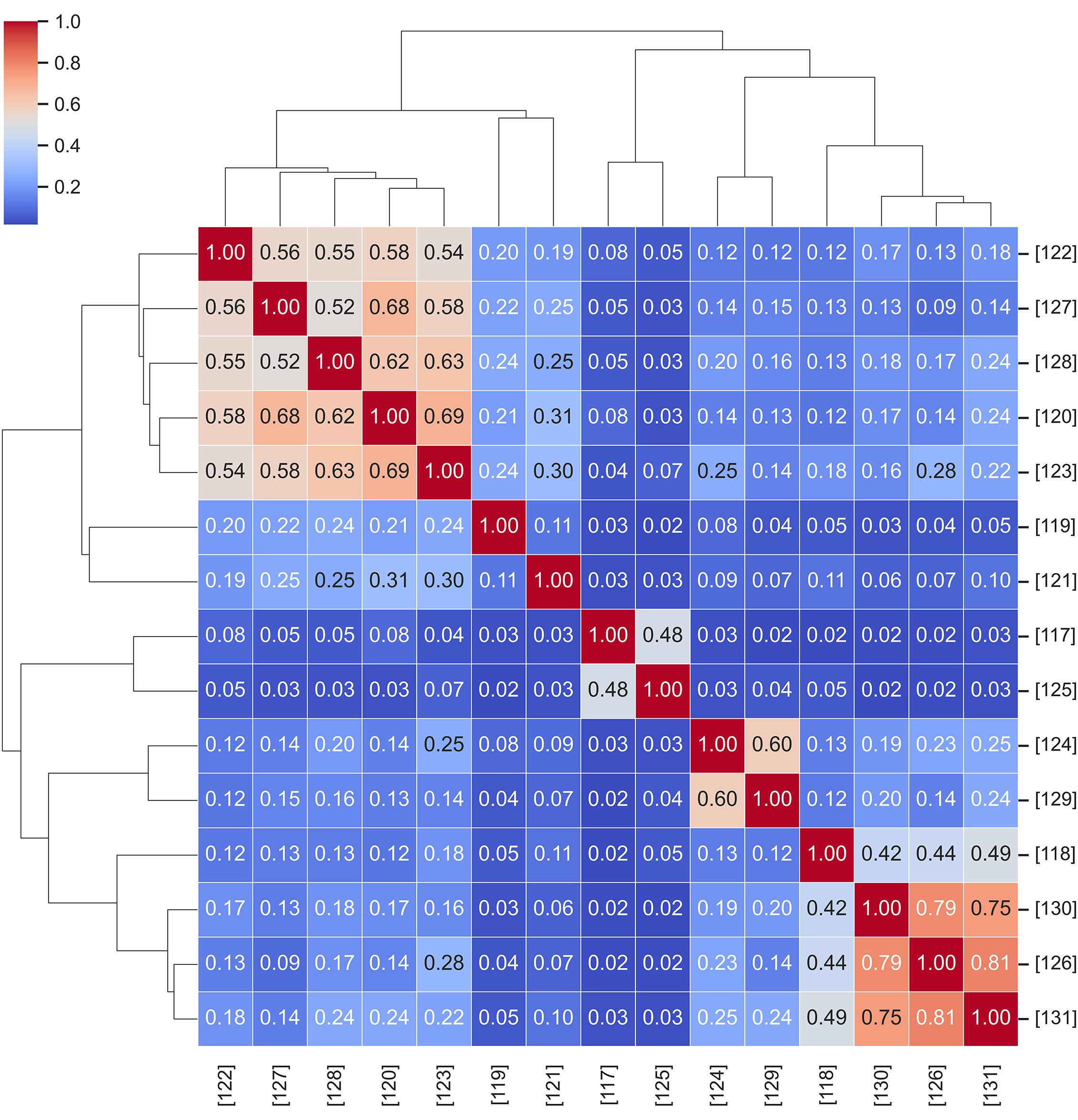
Figure 13: Hierarchical similarity map of graph-based spatiotemporal forecasting studies
The dendrogram structure in Fig. 13 reveals two main clusters. The upper-left branch groups studies [120,122,123,127,128] that emphasize static or semi-dynamic adjacency modeling, where spatial priors are either predefined or updated infrequently. In contrast, the lower-right cluster (e.g., [126,130,131]) aggregates works integrating GSL or attention-based edge refinement, highlighting adaptive graph construction as a key research trajectory. Intermediate clusters (e.g., [117,125]) represent hybrid configurations that combine temporal convolutional encoders with partially learnable connectivity, bridging the gap between predefined topology and fully data-driven edge inference.
These textual proximities mirror the methodological trends summarized in Table 8, suggesting that recent advances in dynamic message passing, multi-scale temporal aggregation, and edge-aware learning are increasingly interrelated across application domains such as wind, PV, and load forecasting. By embedding linguistic similarity into a hierarchical structure, Fig. 13 provides readers with a systematic guide to navigate related works—clarifying which models share comparable architectural assumptions and which diverge through novel spatiotemporal adaptations.
To visualize the conceptual structure of graph-based spatiotemporal learning, Fig. 14 depicts a two-dimensional keyword landscape projected by PCA over cosine similarity embeddings. Each point represents a high-frequency term extracted from the reviewed corpus, with color denoting its cluster membership and size reflecting relative TF-IDF weight.
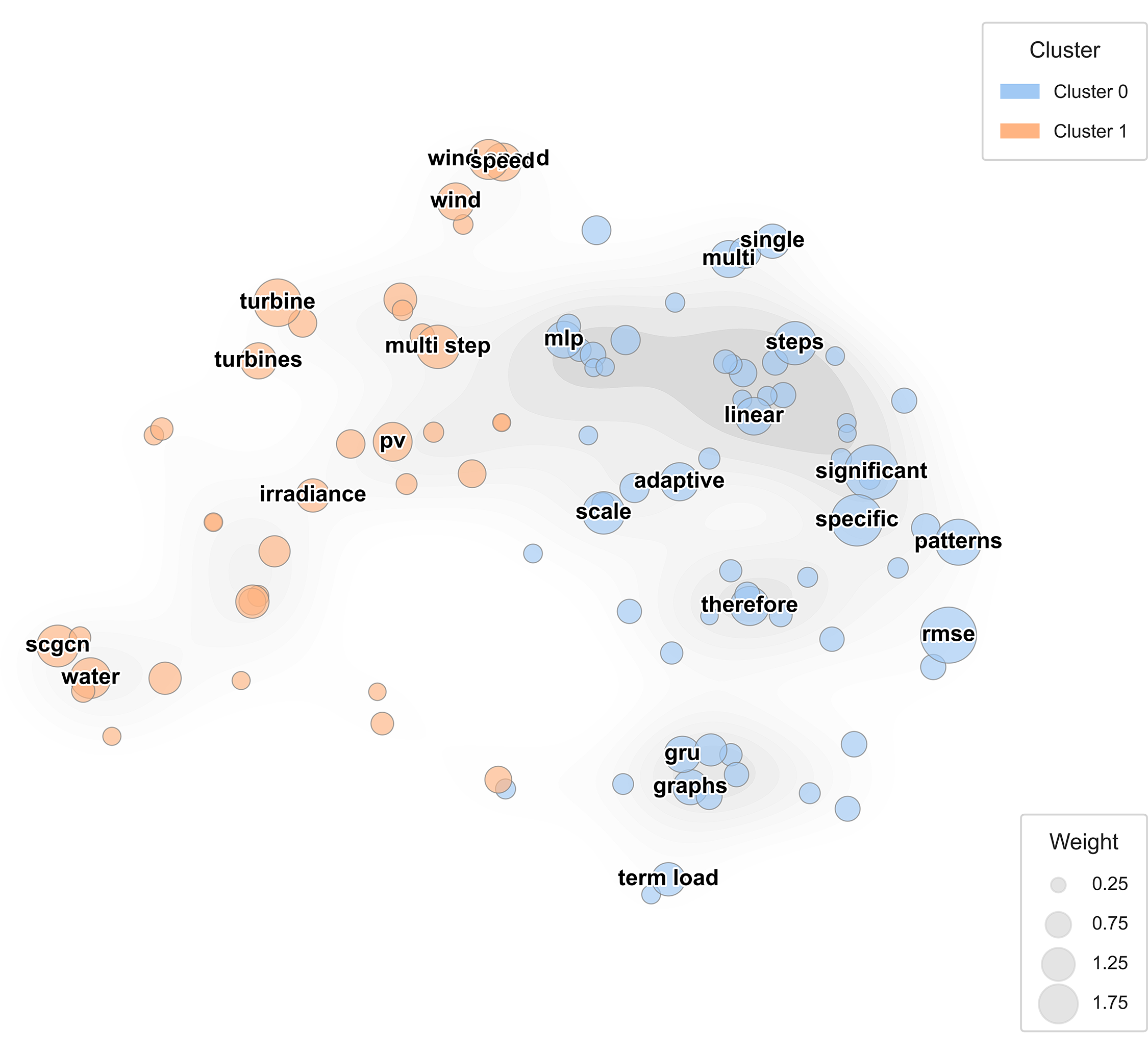
Figure 14: Keyword landscape of graph-based spatiotemporal learning in cold-start forecasting
Fig. 14 separates the underlying vocabularies that shape current research trajectories. In the visualization, the orange cluster consolidates terms associated with physical system components—such as turbine and irradiance—whereas the blue cluster groups concepts tied to computational modeling, including adaptive and scale. This spatial differentiation underscores the inherently hybrid character of ST-GNNs: their effectiveness stems from weaving together physical domain insight with data-driven optimization techniques, thereby narrowing the semantic divide between engineering intuition and algorithmic learning. This side of the map highlights studies that focus on generic learning structures such as GRU, MLP, and graph aggregation, aiming to refine computational efficiency and predictive generalization under cold-start conditions.
Collectively, the spatial arrangement in Fig. 14 illustrates how energy-specific and method-oriented vocabularies converge within the modern ST-GNN framework. It visually reinforces the dual emphasis discussed in Section 5: (1) capturing spatial relationships through graph topology, and (2) leveraging adaptive temporal modules for robust, low-data forecasting. Such conceptual clustering provides empirical support for the field’s transition toward unified, cross-domain spatiotemporal learning paradigms.
The following contributions in this area are the most notable. Yang et al. [129] introduced double-explored spatiotemporal graph neural network (DEST-GNN), a graph neural network (GNN) that predicts intra-hour PV output for multiple sites by modeling spatiotemporal correlations with undirected graphs and sparse attention. On NREL datasets from Alabama and California, DEST-GNN achieved MAEs of 0.49 and 0.42, outperforming independent and fixed-graph baselines for multi-site PV forecasting.
Yu et al. [115] offered a comprehensive review in 2025, tracing how DL has reshaped time-series and spatiotemporal forecasting across sectors such as energy, weather, transportation, and healthcare. Their analysis showed that advanced models—particularly spatiotemporal GNNs and transformers—were driving clear improvements in predictive performance. The review also emphasized practical considerations, including the need for high-quality datasets, thoughtful allocation of computational resources, and attention to model scalability.
Collectively, these studies highlight a critical advantage of the ST-GNNs, their ability to embed spatial coupling directly into the model architecture, enabling meaningful predictions in low-data regimes. Rather than relying solely on fine-tuning or meta-initialization, these models use “reason over neighbors” via learned or structured graph edges, making them a suitable option for forecasting tasks where data are sparse, delayed, or partially missing.
5.3 Cold-Start Deployment Strategies with Spatiotemporal Graph Neural Networks
The ST-GNN introduces a unique architectural bias. By jointly employing a spatial structure and temporal dynamics, these types of networks bypass the need for extensive local labels during deployment, which is useful in energy applications where new sites often lack sufficient telemetry but are surrounded by well-instrumented neighbors [113]. Unlike TL or MAML, which emphasize parameter reuse or fast adaptation, respectively, ST-GNNs directly produce useful forecasts via relational reasoning encoded in graph edges [132].
In a zero-shot setup, the model employs an initial adjacency matrix derived from geographic proximity, electrical topology, or turbine layout to propagate signals via a fixed graph. Eq. (4) handles spatiotemporal aggregation without local gradient updates. As soon as a few samples are gathered, few-shot updates can refine the edge weights or temporal filters using lightweight backpropagation, avoiding the full-network fine-tuning typically required in TL. The following hybrid strategy may also be deployed: 1) initialize global parameters via TL and 2) re-weight edges via ST-GNN message passing to handle local climate or operational differences.
5.4 When and How to Integrate Spatiotemporal Graph Neural Networks
The ST-GNN outperforms TL or MAML under specific cold-start conditions. If a new node has rich neighbors (e.g., a newly added rooftop PV near existing arrays), relational message passing enables useful forecasting without meta-updates. When label scarcity is combined with stable network geometry, which is common in microgrids or industrial feeders, shared edge weights facilitate supervision transfer. Moreover, temporal convolutions allow ST-GNNs to handle subminute ramps that traditional models miss, making them suitable for high-resolution SCADA streams.
Explainability is another strength of such models. Edge attention scores in models (e.g., DEST-GNN or GAT-LSTM) reveal which nodes most influence predictions, enhancing model transparency [128,129]. These features position ST-GNNs as the middle ground between zero-shot TL and few-shot meta-learners. A layered deployment may proceed as follows: Day 0, deploy a zero-shot TL model; Hour 1, switch to a ST-GNN with a fixed graph; Week 1, initiate edge-level fine-tuning; and Season 1, consider full meta-retraining if long-term data justifies the cost. This strategy balances adaptation speed, computational efficiency, and long-term accuracy in real-world systems.
6 Synthetic-Data Generation for Cold-Start Energy Forecasting
In cold-start scenarios (e.g., when a new PV site comes online and only a few hours of sensor data are logged), generative learning enhances model training by enriching the data space rather than optimizing the architecture or weights [133]. When only a single, small dataset is available and no access to related tasks or domains exists, relying solely on these limited observations causes severe overfitting. Instead, generative models synthesize plausible pseudo-data that mirror the statistical structure of the target distribution, expanding coverage before the forecaster even observes real-world samples [16].
This approach is formalized in Eq. (5), where a generative model
The resulting synthetic dataset
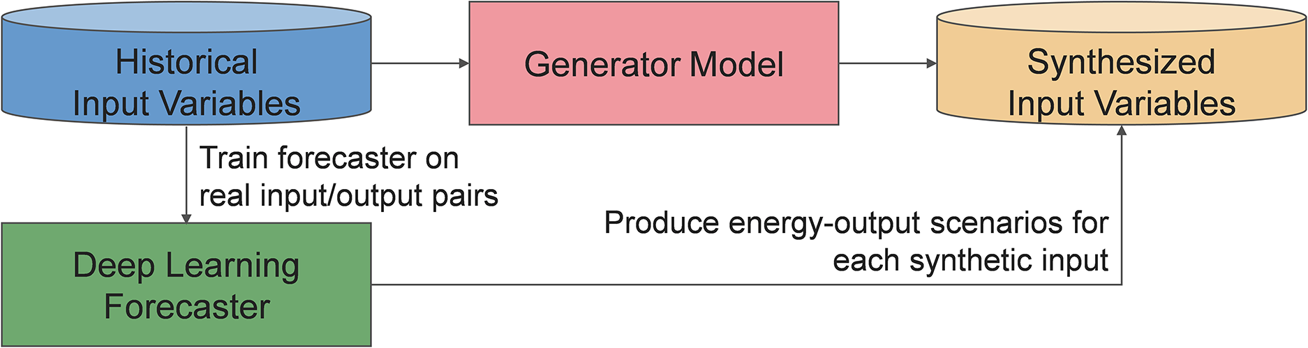
Figure 15: Synthetic-data pipeline for cold-start energy forecasting
This approach allows forecasting models to perform meaningfully even with minimal observed data, a critical advantage in domains (e.g., solar output, wind power, and smart-grid demand) where the ground truth is often delayed or expensive to collect. The sections below introduce critical frameworks, including generative adversarial networks (GANs), TimeGAN, diffusion, and graph-based generators, summarizing recent studies that validate these methods in energy-sector deployments [135–138].
Recent literature has demonstrated the practical value of this strategy across diverse energy applications. Table 9 synthesizes 15 notable studies that apply GANs, diffusion models, and hybrid architectures to domains including PV forecasting, wind power prediction, grid load estimation, and power-flow reconstruction. Each paper quantifies the gains relative to strong nonaugmented baselines, underscoring that, even without dense telemetry, synthetic augmentation can substantially reduce forecast errors and enhance model robustness.
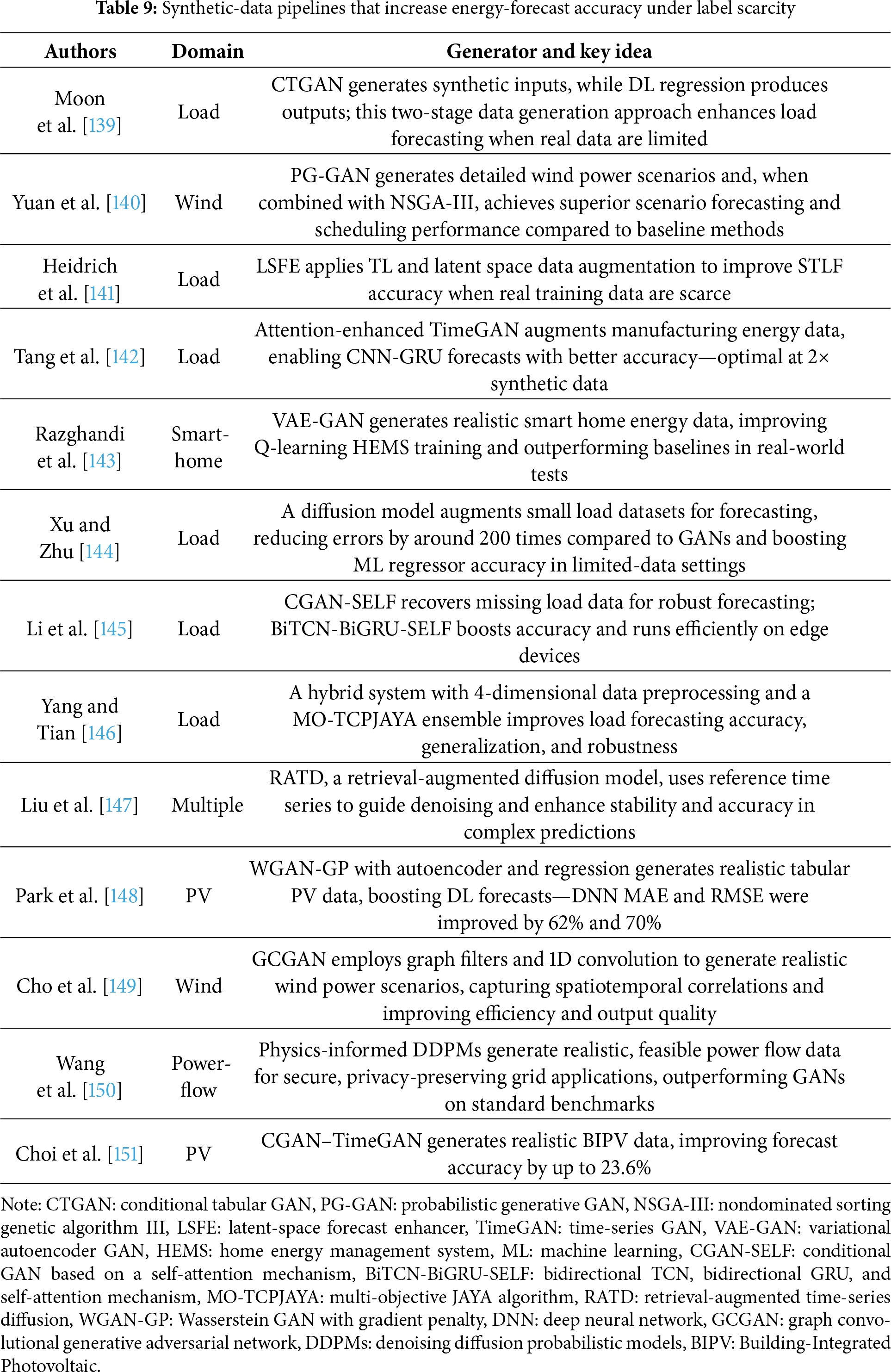
These recent studies collectively highlight the following five notable trends that are reshaping the role of generative learning in cold-start energy forecasting:
• Foundational evidence for GANs in tabular energy data: Early studies have established that generative models (e.g., conditional tabular GAN) can significantly reduce forecasting errors in short-term load forecasting, providing a baseline for advances in synthetic augmentation.
• Integration of physical constraints: Recent work has combined diffusion models with domain-specific knowledge, embedding power-system feasibility into generative architectures. This trend enhances the realism and operational applicability of synthetic data.
• Synergy with TL: Augmentation is increasingly employed to enrich TL pipelines. By populating latent spaces with plausible pseudo-samples, generative methods can help pretrained models generalize more quickly in cold-start settings.
• Privacy-aware augmentation: Generative techniques are also effective in privacy-sensitive contexts. For instance, synthetic consumption traces can replace raw smart-home telemetry during model training without compromising performance.
• Lightweight fallback options: Even simple hybrid schemes combining a few synthetic samples with interpolated data offer measurable improvements, especially when computation or data access is limited. This result makes generative augmentation practical even for edge deployments.
Taken together, these studies chart the progression of generative augmentation in energy forecasting, from initial gains achieved with tabular GANs to recent advances in physics-informed diffusion models and integrated hybrid pipelines that complement TL. These studies substantiate the conceptual foundations of Section 6 and provide actionable references for practitioners, modelers, and energy systems architects aiming to address data scarcity in real-world deployments.
To highlight the linguistic and conceptual structure of recent research on synthetic-data generation for cold-start energy forecasting, Fig. 16 summarizes the twenty most significant keywords extracted from relevant studies. The visualization integrates three statistical dimensions—TF-IDF sum, document frequency, and normalized weight—to capture how core methodological terms recur across the literature.
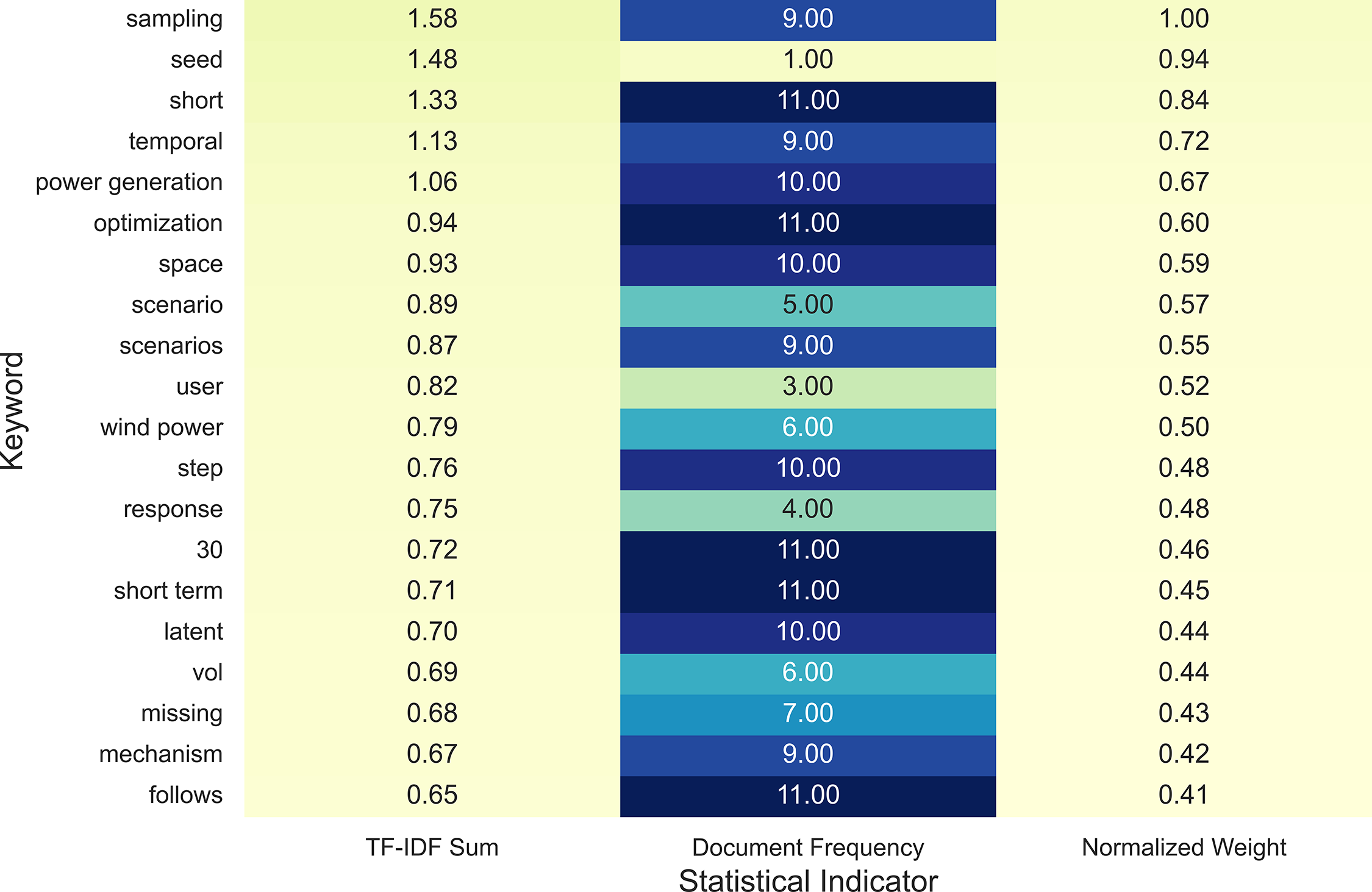
Figure 16: Quantitative summary of dominant keywords in synthetic-data generation for cold-start energy forecasting
The most dominant terms, such as sampling, seed, short, and temporal, emphasize the focus on data scarcity mitigation and short-term forecasting horizons, where synthetic augmentation compensates for limited real-world observations. Keywords like power generation, optimization, and scenario appear with high statistical relevance, indicating a shift toward scenario-based modeling and physically consistent data synthesis, often combining generative and constraint-driven approaches. Terms such as response, latent, and missing reflect the emergence of latent-space modeling and data-imputation mechanisms, both essential for constructing realistic yet privacy-safe synthetic datasets.
Collectively, these linguistic patterns correspond to the practical developments outlined in Table 9, where techniques such as GAN-based tabular augmentation, diffusion-driven denoising, and retrieval-guided synthesis demonstrate measurable forecasting improvements under sparse conditions. The quantitative distribution in Fig. 16 thus reinforces the view that generative learning expands the usable data space rather than altering the predictive architecture itself, positioning it as a complementary paradigm alongside transfer and meta-learning in addressing data scarcity challenges.
To examine the conceptual proximity among recent studies on synthetic-data generation in energy forecasting, Fig. 17 presents a hierarchical similarity map derived from TF-IDF cosine similarity. Each matrix cell quantifies the directional alignment between two studies, while the dendrograms at the top and left illustrate how they cluster according to shared methodological or domain-specific language.
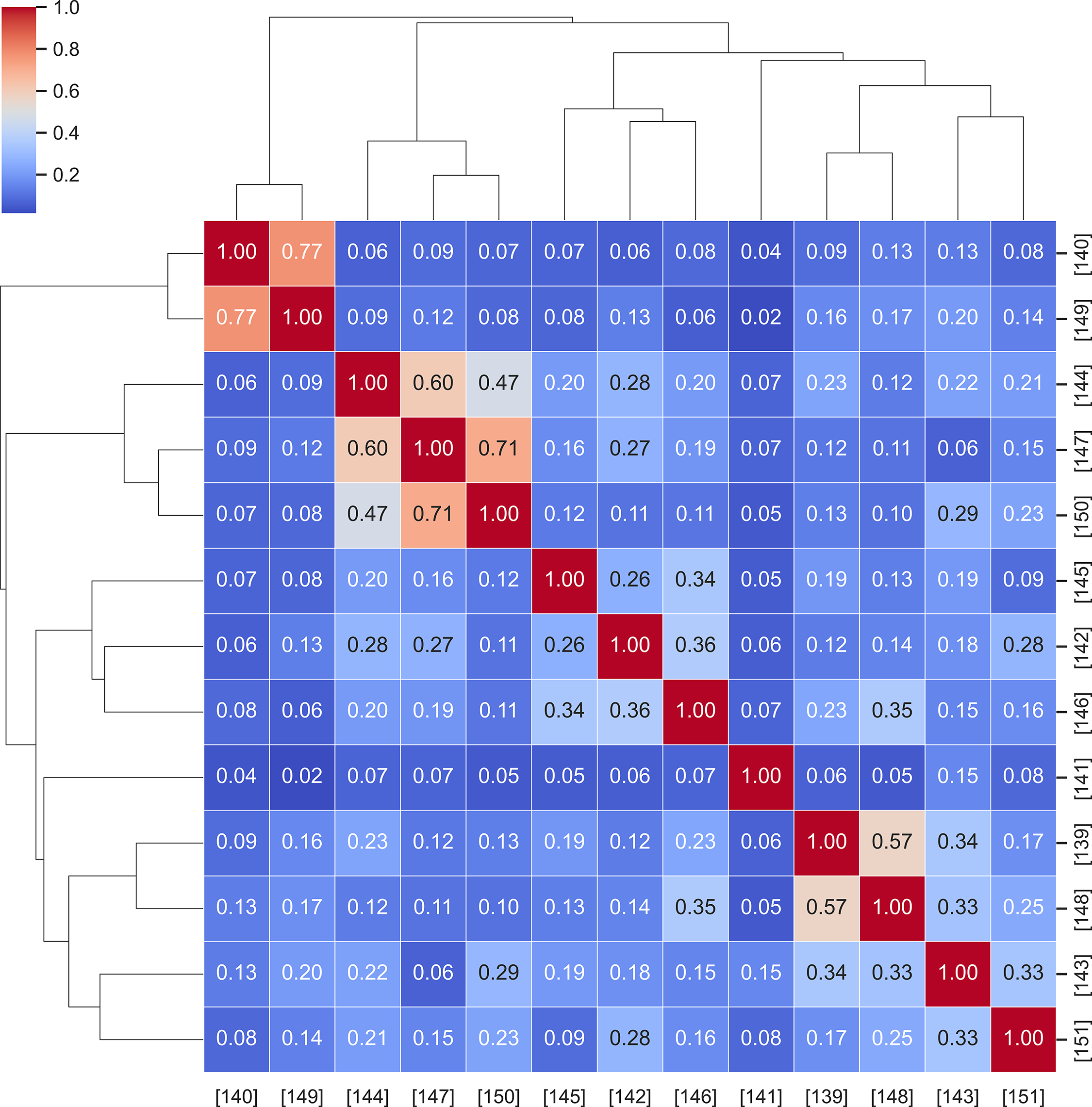
Figure 17: Hierarchical similarity map among synthetic-data generation studies
The hierarchical dendrogram in Fig. 17 outlines the methodological progression that has shaped recent developments in generative modeling. The upper-left branch (e.g., [140,149]) coalesces early adversarial approaches, where conditional generator designs such as PG-GAN formed the initial foundation for synthetic augmentation. Moving toward the center of the hierarchy, a separate cluster (e.g., [144,147,150]) captures the emergence of diffusion-based architectures, making visible the field’s gradual pivot toward more stable, physics-aware denoising processes. Meanwhile, the lower-right region (e.g., [143,148,151]) brings together domain-oriented adaptations—from smart-home simulation to BIPV forecasting—illustrating how these generative frameworks are being reshaped to meet practical deployment requirements.
This hierarchical arrangement mirrors the methodological progression summarized in Table 9: from early GAN-based tabular synthesis toward diffusion-driven hybrid frameworks that integrate domain constraints, privacy preservation, and transferability. By capturing these relationships through textual similarity, Fig. 17 helps readers identify which works share underlying design principles and which extend the generative paradigm into new data modalities. Such a structural view reinforces the interpretive goal of Section 6—showing how synthetic-data generation has matured into a coherent research direction that complements transfer and meta-learning in addressing data scarcity.
To visualize how recent generative-learning studies organize conceptually across the cold-start forecasting domain, Fig. 18 maps the high-frequency keywords in a two-dimensional PCA projection derived from cosine-similarity embeddings. Each color represents a distinct cluster of research emphasis, while the circle size indicates each term’s relative TF-IDF weight within the corpus.
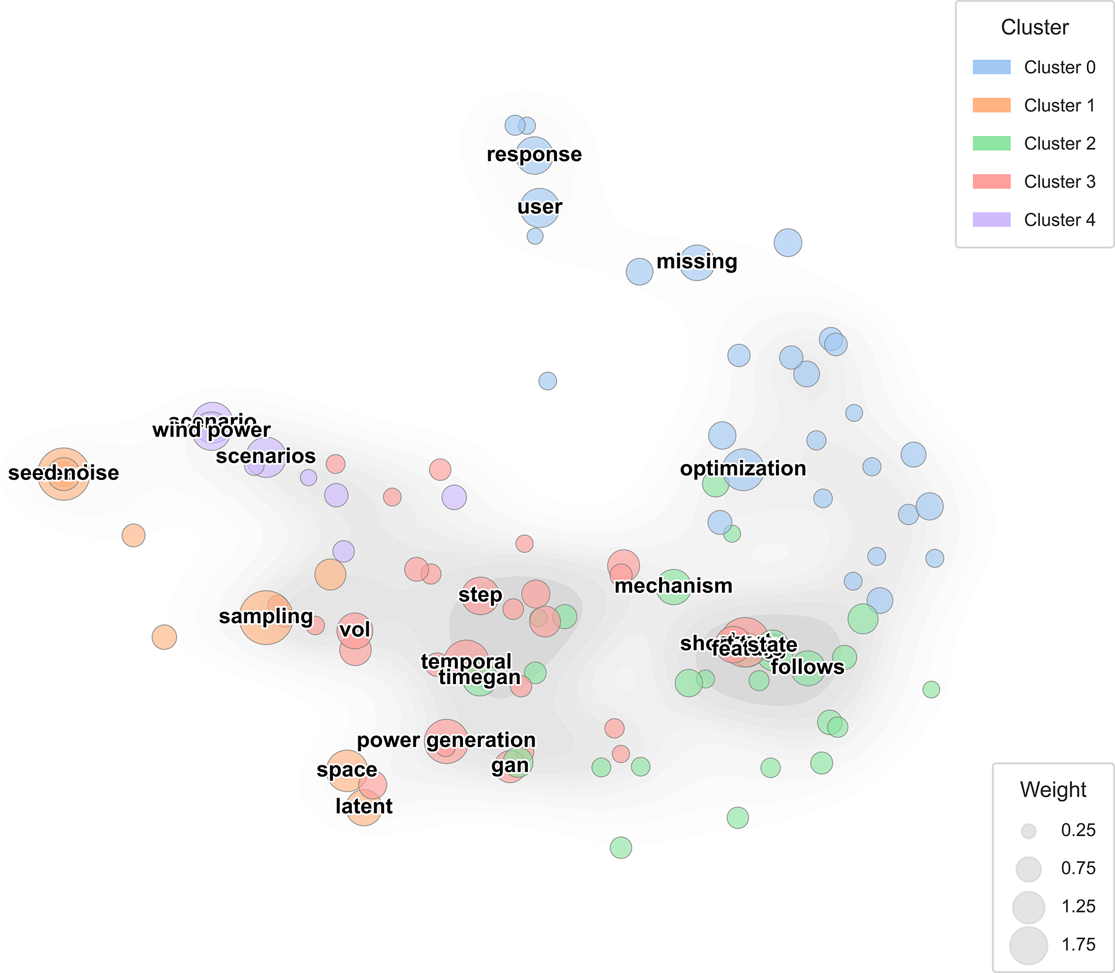
Figure 18: Hierarchical similarity map among synthetic-data generation studies
Five primary conceptual regions emerge. The blue cluster (Cluster 0) groups structural and operational terms—optimization, response, and user—reflecting studies focused on algorithmic stability, model tuning, and feedback-driven control in energy forecasting frameworks. The orange cluster (Cluster 1) centers on sampling, seed, and noise, signifying data-generation mechanics and stochastic training pipelines found in GAN-based and diffusion-based synthesis. The red cluster (Cluster 3) encompasses temporal, power generation, and GAN, pointing to time-series-driven generation models (e.g., TimeGAN, conditional GANs) that simulate dynamic energy behavior. The green cluster (Cluster 2) collects mechanism, state, and follows, aligning with rule-constrained or physics-informed architectures that embed domain feasibility into synthetic data. Finally, the purple cluster (Cluster 4) connects scenario and wind power, representing application-level scenario modeling for renewable-energy systems and grid-planning studies.
The spatial separation among clusters reveals how the field has diversified from early GAN-centric augmentation toward hybrid and domain-integrated generation pipelines that combine temporal dynamics, physical realism, and optimization feedback. Thus, the conceptual landscape in Fig. 18 complements the hierarchical similarity structure in Fig. 17 by showing the underlying semantic relationships among core methodological vocabularies. Together, these analyses demonstrate that generative augmentation is evolving into an independent yet interoperable pillar of data-driven energy forecasting.
6.2 Using Generative Learning under Cold-Start Constraints
Although TL and meta-learning frameworks have demonstrated notable efficacy in adapting models across tasks, these frameworks remain contingent upon the availability of labeled data at the target site. However, the initiation of energy systems often occurs in environments devoid of telemetry or with only a limited number of labeled samples available. Generative learning circumvents this bottleneck by generating statistically coherent pseudo-samples prior to supervised training [152]. In scenarios where local labels are unavailable, GANs or diffusion-based models can be applied to generate realistic inputs, enabling training to commence from Day 0. Conversely, substantial adaptation by TL and MAML necessitates a minimum of 5 to 30 examples.
Furthermore, generative pipeline implementation has great potential for accentuating rare yet critical events (e.g., extreme solar ramps or grid faults), which are commonly underrepresented in historical records. By deliberately oversampling these outlier cases, models can be rendered more robust in their ability to predict extreme behavior. Privacy and deployment constraints favor this strategy [153]. In residential or commercial settings where data sharing is prohibited, pretrained generators (rather than raw logs) can be transferred across domains. Furthermore, synthetic augmentation can be executed off-line, preserving the lightweight nature of the deployed inference model, which is critical in edge computing environments, where resources (e.g., random access memory and power) are constrained [154].
6.3 Canonical Formulation and Forecasting Integration
In scenarios where historical telemetry data are limited (e.g., for newly installed PV systems or emerging microgrids), the cold-start problem substantially impedes accurate energy forecasting. A promising remedy is applying generative models, particularly those trained under a Wasserstein-style objective, which enhances the training stability and output realism. The optimization problem is formulated as in Eq. (6):
where
From the cold-start perspective, generator
7 Conversational Natural Language Processing and Explainable-AI Interfaces
The importance of transparency and human interpretability increases as these forecasting systems scale and influence critical infrastructure decisions [155]. Integrating XAI modules helps stakeholders understand how synthetic data affect model outcomes, building trust [156]. Furthermore, chatbot interfaces driven by natural language processing enable nonexperts (e.g., grid operators or policymakers) to query models interactively, audit decisions, and interpret forecasts in real time [31]. Such interfaces democratize access to complex AI systems, ensuring ethical, auditable, and inclusive decision-making in data-scarce energy contexts.
7.1 Bridging Cold-Start Forecasts to the Control-Room Operator
Although LLMs and interactive XAI dashboards do not improve raw accuracy as directly as MAML, TL, or ST-GNNs, they determine whether human users trust and act on the model output. This section surveys nine recent systems that provide PV/wind/load forecasters with dialogue agents, multimodal LLM pipelines, or web-based explanation panels. Each study is evaluated on the following three axes:
• Dialogue utility refers to how naturally users can interact with forecasting systems via language, including asking open-ended questions (e.g., “Why is tomorrow’s solar output lower?”), applying small data updates (few-shot correction), and obtaining real-time advice (e.g., “Activate storage if output falls below 20 kW”).
• The XAI depth measures the clarity of the reasoning of the model. Critical XAI tools include 1) Shapley additive explanations (SHAP), demonstrating the contribution of each input to a prediction; 2) local interpretable model-agnostic explanations (LIME), using simple models to explain individual predictions; and 3) gradient-weighted class activation mapping (Grad-CAM), highlighting the most influential input areas in CNNs.
• Operational lift encompasses practical performance gains beyond standard accuracy metrics. Examples include reductions in forecast variance, mitigation of hallucinations in natural language generation, and improvements in human-in-the-loop processes (e.g., accelerated fault diagnosis and reduced operator errors) enabled by interpretable feedback from AI systems.
Table 10 presents a curated chronology of landmark systems combining interactive natural language processing and XAI in the context of energy forecasting. Spanning from 2020 to 2025, the table highlights state-of-the-art research that has shifted from static dashboards to dynamic, dialogue-based interfaces.
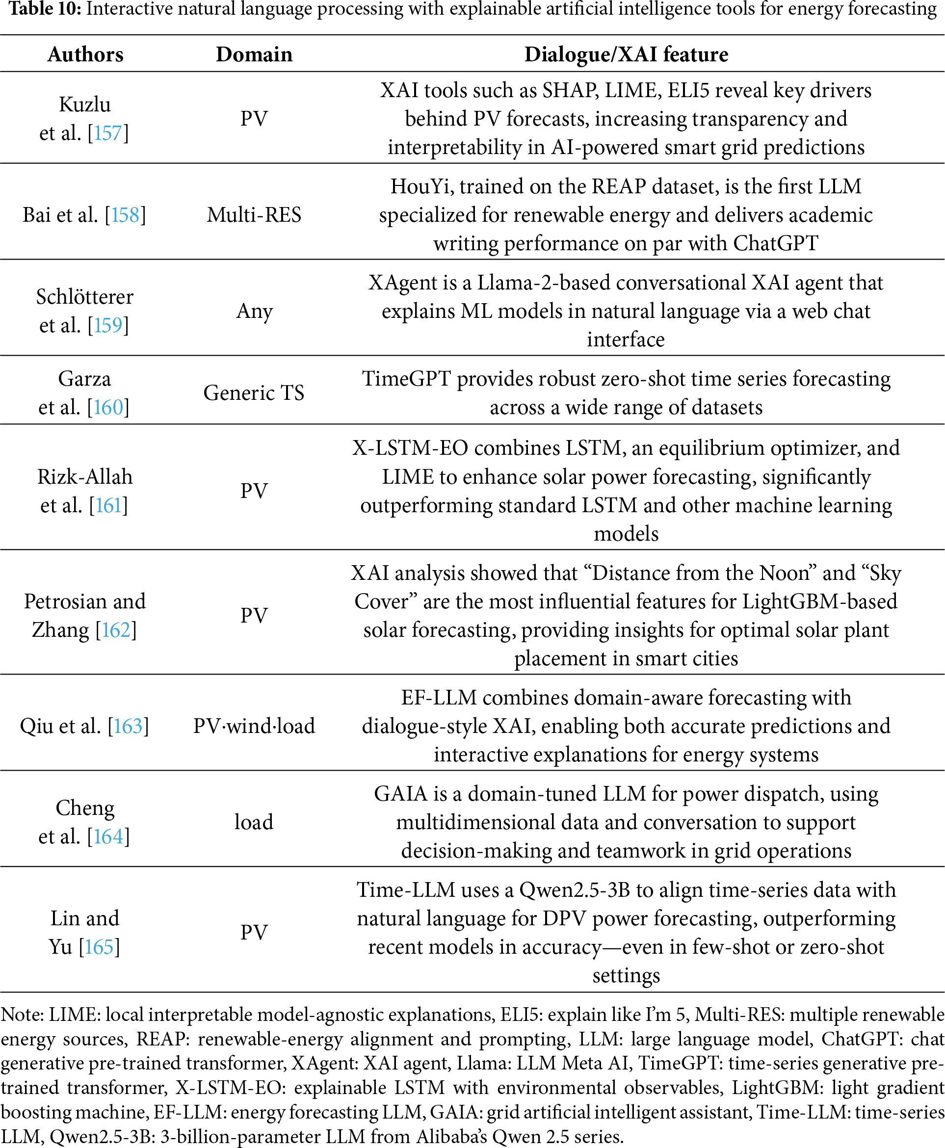
7.2 Conversational XAI for Cold-Start Interpretability
In newly activated solar PV sites, where historical performance data are often limited or absent, forecasting tools must contend with more than just modeling uncertainty. A critical challenge during this emerging stage is to ensure that users, ranging from technical staff to operations managers, can interpret and have confidence in the predictions they receive. Rather than relying exclusively on statistical metrics, success in these scenarios is contingent on the capacity of the system to articulate its reasoning in a transparent and pragmatic manner.
Conversational XAI platforms are assuming this role by providing interactive, question-driven explanations customized to user queries [166]. For instance, we consider a scenario in which a site supervisor is tasked with reviewing a forecast indicating a sudden decline in expected output around mid-afternoon. Without a sufficiently extensive database for comparison, the supervisor may pose the following query to the system: The objective of this investigation is to ascertain the cause of the predicted decline at 2 pm. Rather than returning abstract probabilities or dense graphs, the interface can respond with a concise explanation, which would cite the rising panel temperature and thickening cloud layers as contributing factors and display a ranked breakdown of input variables for additional clarity. This approach is predicated on the principle of minimizing guesswork.
This functionality is also advantageous for field technicians, particularly in responding to irregular readings. In a standard scenario, a technician might enquire into the potential causes of a generation shortfall, focusing on determining whether the problem can be attributed to weather interference or a technical malfunction [167]. The indication of a voltage spike on one of the inverters suggests the necessity of a hardware inspection, which would facilitate the differentiation between model behavior and equipment problems. In summary, during the preliminary implementation stages, when confidence in AI-driven forecasts is still developing, these conversational tools offer more than convenience. These layers function as critical support layers, facilitating the comprehension, verification, and implementation of complex model outputs across diverse operational roles.
Energy forecasting has traditionally relied on deterministic prediction, providing a single “best-guess” trajectory. Yet modern power systems operate under pervasive uncertainty, where grid operators, traders, and control agents must respond not only to mean expectations but to distributions of risk. Bridging this gap between deterministic modeling and probabilistic reasoning is no longer a technical improvement—it represents a conceptual turning point in how forecasting intelligence should be designed. Cold-start forecasting, in particular, embodies this shift: it is not simply about making early predictions, but about learning to reason when historical experience is absent.
The synthesis presented in Sections 3–7 reveals three complementary strategies—label-efficient learning, probabilistic forecasting, and human-centric interpretability—that together redefine how forecasting pipelines can evolve. These approaches collectively transform static models into adaptive, self-explaining systems capable of operating before sufficient data exist and improving as data accumulate. In doing so, they establish a design framework for next-generation forecasting systems: architectures that can generalize beyond their training domain, quantify their uncertainty, and translate predictions into actionable human insight. Table 11 summarizes these strategies and their practical implications.
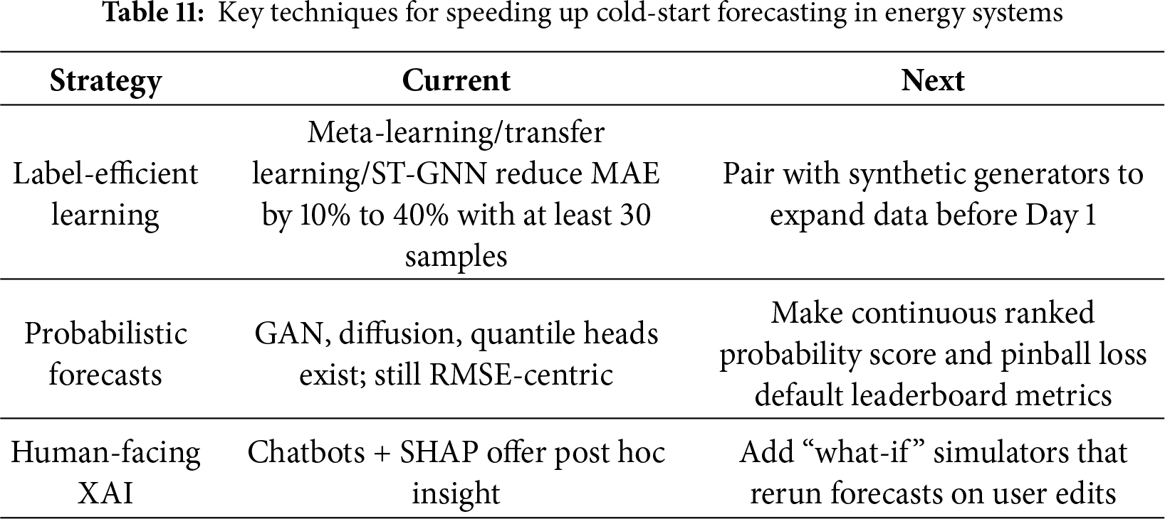
Three guiding insights emerge from this synthesis.
• First, data scarcity should be treated as a design principle rather than a constraint. Meta-learning, TL, and ST-GNN architectures demonstrate that limited data can be transformed into inductive structure, allowing models to encode meaningful relational priors instead of statistical noise.
• Second, uncertainty is the language of reliable forecasting. Metrics such as CRPS and pinball loss should replace purely point-based measures, acknowledging that forecast confidence often matters more than forecast precision.
• Third, interpretability has become a prerequisite for operational trust. Human-facing XAI interfaces—ranging from conversational agents to interactive “what-if” simulators—connect algorithmic logic with human decision-making, allowing operators to understand and refine machine forecasts in real time.
Despite this progress, two systemic challenges continue to limit the field.
• The first concerns multimodal fusion in data-scarce environments. Although weather reanalysis, sky imagery, and SCADA telemetry provide complementary signals, few systems can yet integrate these sources coherently during the cold-start phase. Effective multimodal forecasting will require probabilistic fusion architectures capable of propagating uncertainty across heterogeneous modalities rather than treating them as deterministic inputs.
• The second challenge lies in benchmark fragmentation. Divergent datasets, forecasting horizons, and evaluation metrics across solar, wind, and load domains hinder comparability and reproducibility. A unified, federated benchmarking ecosystem—combining advanced data generation techniques and collaborative strategies—is essential for transforming fragmented progress into collective intelligence [168].
A further emerging issue is the sustainability of learned knowledge over time. As forecasting models continually adapt through TL or meta-learning, they also risk accumulating obsolete or biased representations. Recent advances in machine unlearning provide a promising mechanism for maintaining model integrity by selectively removing outdated knowledge without full retraining. In the context of renewable forecasting, unlearning could enable systems to discard region-specific biases or outdated seasonal patterns, ensuring that adaptation remains reliable even as data distributions evolve [169–171]. Integrating unlearning with cold-start learning would thus complete the data-lifecycle loop—learning efficiently under scarcity and forgetting responsibly under change.
Although cold-start pressures are most acute for solar PV and wind power, extending label-efficient learning pipelines to other renewables remains promising. In hydropower, coupling basin-scale hydrology with long-lead inflow forecasts may shift the main challenge from data scarcity to regime shifts and extremes [172]. Emerging hybrid or “firm” portfolios—linking variable and dispatchable resources such as wind–hydro, PV–battery, and bioenergy systems—are already blurring the boundary between stochastic and controllable generation [173,174]. These developments open new possibilities to pair transfer and meta-learning with resource co-optimization, broadening cold-start forecasting and supporting more adaptive, low-carbon power systems.
Ultimately, this review proposes that the evolution of energy forecasting should not be measured by data volume or model complexity, but by how gracefully systems learn, adapt, and unlearn in dynamic environments. The intelligence of future energy systems will not reside in the quantity of information they remember, but in their capacity to revise, recalibrate, and imagine what has not yet been observed.
Over the past decade, energy forecasting has evolved from data-intensive DL pipelines into label-efficient, uncertainty-aware, and interpretable architectures capable of operating under data scarcity. What once depended on massive labeled datasets has matured into a discipline of strategic adaptation, where models learn to reason under limited experience. This transformation represents not merely a technical refinement but a conceptual shift—from prediction as memorization to prediction as understanding in the face of uncertainty.
Recent advances have equipped forecasting systems with mechanisms for rapid and adaptive learning.
• In the earliest stage of cold-start forecasting, zero-, few-shot, and meta-learning redefine what learning efficiency means. These approaches allow a model to adapt in less than an hour with as few as 5–30 samples—something previously thought unrealistic. As telemetry grows, routine TL fine-tuning helps the system recalibrate itself naturally, creating a rhythm of continuous adaptation instead of one-time training.
• TL, in practice, remains the quickest entry point for real deployment. It performs well with little computation, requiring just a single gradient pass and almost no manual tuning. Yet, it still struggles when the environment or network topology shifts. Here, ST-GNNs close that gap: by internalizing spatial patterns and relational cues, they enable the model to extend predictive power to new or unobserved nodes without needing a local history.
• Synthetic data generators add another layer of resilience. By simulating rare events and long-tail patterns that rarely appear in actual records, they expand the model’s horizon and stabilize performance under unexpected conditions. In short, synthetic generation prepares models not only for what has happened, but for what might.
• Lastly, conversational LLM and XAI components turn dense numerical outputs into explanations that people can reason with. These layers make forecasts interpretable in real time, allowing human operators to test “what-if” scenarios, challenge outcomes, and refine strategies. The result is a forecasting system that does not just predict—it collaborates.
The cold-start deployment of forecasting systems for new renewable assets—such as solar PV farms, wind installations, and microgrids—requires a staged, self-improving framework. On the first day of operation, before meaningful local data exist, a zero-shot TL backbone combined with a graph-aware model (e.g., ST-GNN) can leverage physical topology or historical connectivity to produce baseline predictions. As data begin to accumulate, GAN- or diffusion-based models can synthesize pseudo-samples for few-shot fine-tuning through lightweight adaptation mechanisms such as low-rank updates or meta-learning. By the end of the first operational month, probabilistic ST-GNNs or transformer-based models can be retrained using real and synthetic data, forming a robust forecasting backbone. At this stage, interpretability layers (e.g., SHAP or LIME) and LLM-driven natural language interfaces transform forecasts into actionable and human-understandable explanations.
From a broader perspective, this review highlights several policy and research implications.
• Regulatory frameworks now need to move beyond point forecasts. Adopting calibrated probabilistic outputs would introduce transparency and accountability directly into operational decision-making, ensuring that every new renewable connection includes quantified uncertainty as part of its forecast.
• At the same time, collaboration across institutions demands privacy by design. Federated validation and synthetic-data testing can make large-scale benchmarking possible without ever exposing private SCADA streams. Open, version-controlled benchmark suites following these principles would finally make comparability and reproducibility a default, not an afterthought.
• The next decade of forecasting will depend on cooperation across disciplines—machine learning, power systems, human–computer interaction, and uncertainty quantification. These intersections are where the most durable ideas form. Progress will favor architectures that are not just accurate but transparent; not just automated but ethically grounded and explainable at scale.
As forecasting models continue to evolve, they must also learn to unlearn. Continuous adaptation without selective forgetting risks perpetuating outdated or biased patterns. Recent research on machine unlearning provides a mechanism for maintaining model integrity—allowing systems to discard obsolete or context-specific knowledge without full retraining. In dynamic environments marked by shifting climates, market structures, and policy regimes, unlearning will become as essential as learning itself. Integrating cold-start learning with unlearning completes the full data lifecycle—learning efficiently from scarcity, adapting through change, and forgetting responsibly when knowledge becomes obsolete.
Looking forward, forecasting will play a pivotal role in navigating the climate and energy transition. As global warming accelerates and extreme events challenge predictability, the ability to anticipate—not just the likely but the newly possible—will define the resilience of modern energy systems. The next generation of forecasting will rely on self-healing algorithms, physics-informed neural models, digital twins of power grids, and lifelong learning architectures that sustain accuracy under environmental volatility. Ultimately, the intelligence of future energy systems will not depend on the scale of their data or depth of their networks, but on their capacity to sense instability, adapt autonomously, and preserve human agency amidst uncertainty.
Cold-start forecasting, in this light, is not merely an engineering challenge—it represents a new philosophy of sustainable intelligence: one that learns from scarcity, adapts to change, and unlearns the obsolete, guiding society toward a resilient, data-aware, and climate-conscious future.
Acknowledgement: The author would like to express sincere gratitude to Dr. Sungwoo Park from Chung-Ang University for generously sharing his expertise in cold-start energy forecasting. His thoughtful advice and constructive feedback were invaluable in shaping both the conceptual framework and the final presentation of this work.
Funding Statement: The author received no specific funding for this study.
Availability of Data and Materials: All data generated or analyzed during this study are included in this published article.
Ethics Approval: Not applicable.
Conflicts of Interest: The author declares no conflicts of interest to report regarding the present study.
Abbreviations
| ARIMA | Autoregressive integrated moving average |
| AutoML | Automated machine learning |
| BiGRU | Bidirectional gated recurrent unit |
| BIPV | Building-integrated photovoltaics |
| CGAN | Conditional generative adversarial network |
| CNN | Convolutional neural network |
| CORAL | Correlation alignment |
| DANN | Domain-adversarial neural network |
| DEST-GNN | Double-explored spatiotemporal graph neural network |
| DL | Deep learning |
| DNI | Direct normal irradiance |
| ESN | Echo-state network |
| FAF | Feature-adaptive framework |
| GAN | Generative adversarial network |
| GAT | Graph attention network |
| GCN | Graph convolutional network |
| GRU | Gated recurrent unit |
| GSL | Graph structure learning |
| GWNet | Graph WaveNet |
| LIME | Local interpretable model-agnostic explanations |
| LoRA | Low-rank adaptation |
| LSTM | Long short-term memory |
| MALPE | Mean absolute log percentage error |
| MAML | Model-agnostic meta-learning |
| MAPE | Mean absolute percentage error |
| MAE | Mean absolute error |
| N-BEATS | Neural Basis Expansion Analysis |
| nRMSE | Normalized root mean squared error |
| NWP | Numerical weather prediction |
| OLGBM | Optimized light gradient boosting machine |
| PG-GAN | Probabilistic generative GAN |
| PV | Photovoltaic |
| RBM | Restricted Boltzmann machine |
| RMSE | Root mean squared error |
| RNN | Recurrent neural network |
| SCADA | Supervisory control and data acquisition |
| Seq2seq | Sequence-to-sequence |
| SHAP | Shapley additive explanations |
| ST-GNN | Spatiotemporal graph neural network |
| TCN | Temporal convolutional network |
| TFT | Temporal fusion transformer |
| TimeGAN | Time-series generative adversarial network |
| TL | Transfer learning |
| VAE-GAN | Variational autoencoder GAN |
| Wind-TSGNN | Wind temporal-spectral graph neural network |
| XAI | Explainable artificial intelligence |
References
1. Cavus M. Advancing power systems with renewable energy and intelligent technologies: a comprehensive review on grid transformation and integration. Electronics. 2025;14(6):1159. doi:10.3390/electronics14061159. [Google Scholar] [CrossRef]
2. Wen J, Wang Z. Short-term power load forecasting with hybrid TPA-BiLSTM prediction model based on CSSA. Comput Model Eng Sci. 2023;136(1):749–65. doi:10.32604/cmes.2023.023865. [Google Scholar] [CrossRef]
3. Ukoba K, Olatunji KO, Adeoye E, Jen TC, Madyira DM. Optimizing renewable energy systems through artificial intelligence: review and future prospects. Energy Environ. 2024;35(7):3833–79. doi:10.1177/0958305x241256293. [Google Scholar] [CrossRef]
4. Moon J, Kim J, Kang P, Hwang E. Solving the cold-start problem in short-term load forecasting using tree-based methods. Energies. 2020;13(4):886. doi:10.3390/en13040886. [Google Scholar] [CrossRef]
5. Alharbi FR, Csala D. A seasonal autoregressive integrated moving average with exogenous factors (SARIMAX) forecasting model-based time series approach. Inventions. 2022;7(4):94. doi:10.3390/inventions7040094. [Google Scholar] [CrossRef]
6. Shukla S, Hong T. BigDEAL challenge 2022: forecasting peak timing of electricity demand. IET Smart Grid. 2024;7(4):442–59. doi:10.1049/stg2.12162. [Google Scholar] [CrossRef]
7. Park MJ, Yang HS. Comparative study of time series analysis algorithms suitable for short-term forecasting in implementing demand response based on AMI. Sensors. 2024;24(22):7205. doi:10.3390/s24227205. [Google Scholar] [PubMed] [CrossRef]
8. Husein M, Gago EJ, Hasan B, Pegalajar MC. Towards energy efficiency: a comprehensive review of deep learning-based photovoltaic power forecasting strategies. Heliyon. 2024;10(13):e33419. doi:10.1016/j.heliyon.2024.e33419. [Google Scholar] [PubMed] [CrossRef]
9. Ramos PVB, Villela SM, Silva WN, Dias BH. Residential energy consumption forecasting using deep learning models. Appl Energy. 2023;350:121705. doi:10.1016/j.apenergy.2023.121705. [Google Scholar] [CrossRef]
10. Ahmed SF, Alam MSB, Hassan M, Rozbu MR, Ishtiak T, Rafa N, et al. Deep learning modelling techniques: current progress, applications, advantages, and challenges. Artif Intell Rev. 2023;56(11):13521–617. doi:10.1007/s10462-023-10466-8. [Google Scholar] [CrossRef]
11. Fatemi Z, Huynh M, Zheleva E, Syed Z, Di X. Mitigating cold‐start problem using cold causal demand forecasting model. In: Proceedings of the Temporal Graph Learning Workshop @NeurIPS 2023; 2023 Dec 16; New Orleans, LA, USA. [Google Scholar]
12. Xie C, Tank A, Greaves-Tunnell A, Fox E. A unified framework for long range and cold start forecasting of seasonal profiles in time series. arXiv:1710.08473. 2017. [Google Scholar]
13. Xiao F, Liu L, Han J, Guo D, Wang S, Cui H, et al. Meta-learning for few-shot time series forecasting. J Intell Fuzzy Syst. 2022;43(1):325–41. doi:10.3233/jifs-212228. [Google Scholar] [CrossRef]
14. Weber M, Auch M, Doblander C, Mandl P, Jacobsen HA. Transfer learning with time series data: a systematic mapping study. IEEE Access. 2021;9:165409–32. doi:10.1109/ACCESS.2021.3134628. [Google Scholar] [CrossRef]
15. Cini A, Marisca I, Zambon D, Alippi C. Graph deep learning for time series forecasting. ACM Comput Surv. 2025;57(12):1–34. doi:10.1145/3742784. [Google Scholar] [CrossRef]
16. Brophy E, Wang Z, She Q, Ward T. Generative adversarial networks in time series: a systematic literature review. ACM Comput Surv. 2023;55(10):1–31. doi:10.1145/3559540. [Google Scholar] [CrossRef]
17. Ying C, Wang W, Yu J, Li Q, Yu D, Liu J. Deep learning for renewable energy forecasting: a taxonomy, and systematic literature review. J Clean Prod. 2023;384:135414. doi:10.1016/j.jclepro.2022.135414. [Google Scholar] [CrossRef]
18. Klaiber J, Van Dinther C. Deep learning for variable renewable energy: a systematic review. ACM Comput Surv. 2024;56(1):1–37. doi:10.1145/3586006. [Google Scholar] [CrossRef]
19. Paletta Q, Terrén-Serrano G, Nie Y, Li B, Bieker J, Zhang W, et al. Advances in solar forecasting: computer vision with deep learning. Adv Appl Energy. 2023;11:100150. doi:10.1016/j.adapen.2023.100150. [Google Scholar] [CrossRef]
20. Wazirali R, Yaghoubi E, Abujazar MSS, Ahmad R, Vakili AH. State-of-the-art review on energy and load forecasting in microgrids using artificial neural networks, machine learning, and deep learning techniques. Electr Power Syst Res. 2023;225:109792. doi:10.1016/j.epsr.2023.109792. [Google Scholar] [CrossRef]
21. Chu Y, Wang Y, Yang D, Chen S, Li M. A review of distributed solar forecasting with remote sensing and deep learning. Renew Sustain Energy Rev. 2024;198:114391. doi:10.1016/j.rser.2024.114391. [Google Scholar] [CrossRef]
22. Eren Y, Küçükdemiral İ. A comprehensive review on deep learning approaches for short-term load forecasting. Renew Sustain Energy Rev. 2024;189(1):114031. doi:10.1016/j.rser.2023.114031. [Google Scholar] [CrossRef]
23. Biswal B, Deb S, Datta S, Ustun TS, Cali U. Review on smart grid load forecasting for smart energy management using machine learning and deep learning techniques. Energy Rep. 2024;12:3654–70. doi:10.1016/j.egyr.2024.09.056. [Google Scholar] [CrossRef]
24. Bouquet P, Jackson I, Nick M, Kaboli A. AI-based forecasting for optimised solar energy management and smart grid efficiency. Int J Prod Res. 2024;62(13):4623–44. doi:10.1080/00207543.2023.2269565. [Google Scholar] [CrossRef]
25. Verdone A, Panella M, De Santis E, Rizzi A. A review of solar and wind energy forecasting: from single-site to multi-site paradigm. Appl Energy. 2025;392:126016. doi:10.1016/j.apenergy.2025.126016. [Google Scholar] [CrossRef]
26. International Energy Agency (IEA). Hydropower special market report: analysis and forecast to 2030. Paris, France: OECD Publishing; 2021. doi:10.1787/07a7bac8-en. [Google Scholar] [CrossRef]
27. International Energy Agency (IEA). Harnessing variable renewables: a guide to the balancing challenge. Paris, France: OECD Publishing; 2011. doi:10.1787/9789264111394-en. [Google Scholar] [CrossRef]
28. Bult SV, Le Bars D, Haigh ID, Gerkema T. The effect of the 18.6-year lunar nodal cycle on steric sea level changes. Geophys Res Lett. 2024;51(8):e2023GL106563. doi:10.1029/2023GL106563. [Google Scholar] [CrossRef]
29. Bird L, Milligan M, Lew D. Integrating variable renewable energy: challenges and solutions. Golden, CO, USA: NREL; 2013. Report No.: NREL/TP-6A20-60451. doi: 10.2172/1097911. [Google Scholar] [CrossRef]
30. Rozon F, McGregor C, Owen M. Long-term forecasting framework for renewable energy technologies’ installed capacity and costs for 2050. Energies. 2023;16(19):6874. doi:10.3390/en16196874. [Google Scholar] [CrossRef]
31. Schneider J. Explainable Generative AI (GenXAIa survey, conceptualization, and research agenda. Artif Intell Rev. 2024;57(11):289. doi:10.1007/s10462-024-10916-x. [Google Scholar] [CrossRef]
32. Tsegaye S, Sanjeevikumar P, Tjernberg LB, Fante KA. Short-term energy forecasting using deep neural networks: prospects and challenges. J Eng. 2024;2024(11):e70022. doi:10.1049/tje2.70022. [Google Scholar] [CrossRef]
33. Hirth L, Ziegenhagen I. Balancing power and variable renewables: three links. Renew Sustain Energy Rev. 2015;50:1035–51. doi:10.1016/j.rser.2015.04.180. [Google Scholar] [CrossRef]
34. Rosales-Asensio E, Diez DB, Sarmento P. Electricity balancing challenges for markets with high variable renewable generation. Renew Sustain Energy Rev. 2024;189:113918. doi:10.1016/j.rser.2023.113918. [Google Scholar] [CrossRef]
35. Shi H, Xu M, Li R. Deep learning for household load forecasting—a novel pooling deep RNN. IEEE Trans Smart Grid. 2018;9(5):5271–80. doi:10.1109/TSG.2017.2686012. [Google Scholar] [CrossRef]
36. Mocanu E, Nguyen PH, Gibescu M, Kling WL. Deep learning for estimating building energy consumption. Sustain Energy Grids Netw. 2016;6:91–9. doi:10.1016/j.segan.2016.02.005. [Google Scholar] [CrossRef]
37. Mehmood MU, Chun D, Zeeshan Han, Jeon H, Chen G, et al. A review of the applications of artificial intelligence and big data to buildings for energy-efficiency and a comfortable indoor living environment. Energy Build. 2019;202(1):109383. doi:10.1016/j.enbuild.2019.109383. [Google Scholar] [CrossRef]
38. Wang H, Yi H, Peng J, Wang G, Liu Y, Jiang H, et al. Deterministic and probabilistic forecasting of photovoltaic power based on deep convolutional neural network. Energy Convers Manag. 2017;153:409–22. doi:10.1016/j.enconman.2017.10.008. [Google Scholar] [CrossRef]
39. Guo W, Xu L, Wang T, Zhao D, Tang X. Photovoltaic power prediction based on hybrid deep learning networks and meteorological data. Sensors. 2024;24(5):1593. doi:10.3390/s24051593. [Google Scholar] [PubMed] [CrossRef]
40. Zang H, Liu L, Sun L, Cheng L, Wei Z, Sun G. Short-term global horizontal irradiance forecasting based on a hybrid CNN-LSTM model with spatiotemporal correlations. Renew Energy. 2020;160:26–41. doi:10.1016/j.renene.2020.05.150. [Google Scholar] [CrossRef]
41. Assaf AM, Haron H, Abdull Hamed HN, Ghaleb FA, Qasem SN, Albarrak AM. A review on neural network based models for short term solar irradiance forecasting. Appl Sci. 2023;13(14):8332. doi:10.3390/app13148332. [Google Scholar] [CrossRef]
42. Zhang J, Yan J, Infield D, Liu Y, Lien FS. Short-term forecasting and uncertainty analysis of wind turbine power based on long short-term memory network and Gaussian mixture model. Appl Energy. 2019;241:229–44. doi:10.1016/j.apenergy.2019.03.044. [Google Scholar] [CrossRef]
43. Bianchi FM, Maiorino E, Kampffmeyer MC, Rizzi A, Jenssen R. Recurrent neural networks for short-term load forecasting: an overview and comparative analysis. Cham, Switzerland: Springer; 2017. doi:10.1007/978-3-319-70338-1. [Google Scholar] [CrossRef]
44. Kong W, Dong ZY, Hill DJ, Luo F, Xu Y. Short-term residential load forecasting based on resident behaviour learning. IEEE Trans Power Syst. 2018;33(1):1087–8. doi:10.1109/TPWRS.2017.2688178. [Google Scholar] [CrossRef]
45. Kong W, Dong ZY, Jia Y, Hill DJ, Xu Y, Zhang Y. Short-term residential load forecasting based on LSTM recurrent neural network. IEEE Trans Smart Grid. 2019;10(1):841–51. doi:10.1109/TSG.2017.2753802. [Google Scholar] [CrossRef]
46. Chen XW, Lin X. Big data deep learning: challenges and perspectives. IEEE Access. 2014;2:514–25. doi:10.1109/ACCESS.2014.2325029. [Google Scholar] [CrossRef]
47. Hewamalage H, Bergmeir C, Bandara K. Recurrent neural networks for time series forecasting: current status and future directions. Int J Forecast. 2021;37(1):388–427. doi:10.1016/j.ijforecast.2020.06.008. [Google Scholar] [CrossRef]
48. Najafabadi MM, Villanustre F, Khoshgoftaar TM, Seliya N, Wald R, Muharemagic E. Deep learning applications and challenges in big data analytics. J Big Data. 2015;2(1):1. doi:10.1186/s40537-014-0007-7. [Google Scholar] [CrossRef]
49. DrivenData. Benchmark: cold-start LSTM for deep learning [Internet]. Boston, MA, USA: DrivenData; 2024 [cited 2025 Jul 30]. Available from: https://drivendata.co/blog/benchmark-cold-start-lstm-deep-learning. [Google Scholar]
50. Ahmed R, Sreeram V, Togneri R, Datta A, Arif MD. Computationally expedient photovoltaic power forecasting: a LSTM ensemble method augmented with adaptive weighting and data segmentation technique. Energy Convers Manag. 2022;258:115563. doi:10.1016/j.enconman.2022.115563. [Google Scholar] [CrossRef]
51. Kim J, Kim H, Kim H, Lee D, Yoon S. A comprehensive survey of deep learning for time series forecasting: architectural diversity and open challenges. Artif Intell Rev. 2025;58(7):216. doi:10.1007/s10462-025-11223-9. [Google Scholar] [CrossRef]
52. Zhou H, Zhang S, Peng J, Zhang S, Li J, Xiong H, et al. Informer: beyond efficient transformer for long sequence time-series forecasting. Proc AAAI Conf Artif Intell. 2021;35(12):11106–15. doi:10.1609/aaai.v35i12.17325. [Google Scholar] [CrossRef]
53. Keutayeva A, Abibullaev B. Data constraints and performance optimization for transformer-based models in EEG-based brain-computer interfaces: a survey. IEEE Access. 2024;12:62628–47. doi:10.1109/ACCESS.2024.3394696. [Google Scholar] [CrossRef]
54. Zhu Q, Han J, Chai K, Zhao C. Time series analysis based on informer algorithms: a survey. Symmetry. 2023;15(4):951. doi:10.3390/sym15040951. [Google Scholar] [CrossRef]
55. Ssekulima EB, Anwar MB, Al Hinai A, El Moursi MS. Wind speed and solar irradiance forecasting techniques for enhanced renewable energy integration with the grid: a review. IET Renew Power Gener. 2016;10(7):885–989. doi:10.1049/iet-rpg.2015.0477. [Google Scholar] [CrossRef]
56. Kemper N, Heider M, Pietruschka D, Hähner J. Forecasting of residential unit’s heat demands: a comparison of machine learning techniques in a real-world case study. Energy Syst. 2025;16(1):281–315. doi:10.1007/s12667-023-00579-y. [Google Scholar] [CrossRef]
57. He Y, Luo F, Ranzi G. Transferrable model-agnostic meta-learning for short-term household load forecasting with limited training data. IEEE Trans Power Syst. 2022;37(4):3177–80. doi:10.1109/TPWRS.2022.3169389. [Google Scholar] [CrossRef]
58. He T, An L, Chen P, Chen J, Feng J, Bzdok D, et al. Meta-matching as a simple framework to translate phenotypic predictive models from big to small data. Nat Neurosci. 2022;25(6):795–804. doi:10.1038/s41593-022-01059-9. [Google Scholar] [PubMed] [CrossRef]
59. Park S, Kim D, Moon J, Hwang E. Zero-shot photovoltaic power forecasting scheme based on a deep learning model and correlation coefficient. Int J Energy Res. 2023;2023:9936542. doi:10.1155/2023/9936542. [Google Scholar] [CrossRef]
60. Ren X, Wang Y, Cao Z, Chen F, Li Y, Yan J. Feature transfer and rapid adaptation for few-shot solar power forecasting. Energies. 2023;16(17):6211. doi:10.3390/en16176211. [Google Scholar] [CrossRef]
61. Sarmas E, Spiliotis E, Stamatopoulos E, Marinakis V, Doukas H. Short-term photovoltaic power forecasting using meta-learning and numerical weather prediction independent long short-term memory models. Renew Energy. 2023;216:118997. doi:10.1016/j.renene.2023.118997. [Google Scholar] [CrossRef]
62. Ouyang P, Chen D, Yang T, Feng S, Jin Z, Xu M. FAF: a feature-adaptive framework for few-shot time series forecasting. arXiv:2506.19567. 2025. [Google Scholar]
63. Tsoumplekas G, Athanasiadis C, Doukas DI, Chrysopoulos A, Mitkas P. Few-shot load forecasting under data scarcity in smart grids: a meta-learning approach. Energies. 2025;18(3):742. doi:10.3390/en18030742. [Google Scholar] [CrossRef]
64. Li Y, Zhang S, Hu R, Lu N. A meta-learning based distribution system load forecasting model selection framework. Appl Energy. 2021;294:116991. doi:10.1016/j.apenergy.2021.116991. [Google Scholar] [CrossRef]
65. Xiao X, Mo H, Zhang Y, Shan G. Meta-ANN—a dynamic artificial neural network refined by meta-learning for short-term load forecasting. Energy. 2022;246:123418. doi:10.1016/j.energy.2022.123418. [Google Scholar] [CrossRef]
66. Wang R, Wu J, Cheng X, Liu X, Qiu H. Enhancing spatiotemporal wind power forecasting with meta-learning in data-scarce environments. Eng Appl Artif Intell. 2025;156:111121. doi:10.1016/j.engappai.2025.111121. [Google Scholar] [CrossRef]
67. Chen F, Yan J, Liu Y, Yan Y, Tjernberg LB. A novel meta-learning approach for few-shot short-term wind power forecasting. Appl Energy. 2024;362:122838. doi:10.1016/j.apenergy.2024.122838. [Google Scholar] [CrossRef]
68. Koivisto M, Das K, Guo F, Sørensen P, Nuño E, Cutululis N, et al. Using time series simulation tools for assessing the effects of variable renewable energy generation on power and energy systems. Wires Energy Environ. 2019;8(3):e329. doi:10.1002/wene.329. [Google Scholar] [CrossRef]
69. Vettoruzzo A, Bouguelia MR, Vanschoren J, Rognvaldsson T, Santosh KC. Advances and challenges in meta-learning: a technical review. IEEE Trans Pattern Anal Mach Intell. 2024;46(7):4763–79. doi:10.1109/TPAMI.2024.3357847. [Google Scholar] [PubMed] [CrossRef]
70. Finn C, Abbeel P, Levine S. Model‐agnostic meta‐learning for fast adaptation of deep networks. In: International Conference on Machine Learning 2017; 2017 Aug 6–11; Sydney, NSW, Australia. p. 1126–35. [Google Scholar]
71. Kirk R, Zhang A, Grefenstette E, Rocktäschel T. A survey of zero-shot generalisation in deep reinforcement learning. J Artif Intell Res. 2023;76:201–64. doi:10.1613/jair.1.14174. [Google Scholar] [CrossRef]
72. Malladi S, Gao T, Nichani E, Damian A, Lee JD, Chen D, et al. Fine‐tuning language models with just forward passes. Adv Neural Inf Process Syst. 2023;36:53038–75. doi:10.48550/arXiv.2305.17333. [Google Scholar] [CrossRef]
73. Elsahar H, Gallé M. To annotate or not? Predicting performance drop under domain shift. In: Proceedings of the 2019 Conference on Empirical Methods in Natural Language Processing and the 9th International Joint Conference on Natural Language Processing (EMNLP-IJCNLP); 2019 Nov 3–7; Hong Kong, China. p. 2163–73. doi:10.18653/v1/D19. [Google Scholar] [CrossRef]
74. Oreshkin BN, Carpov D, Chapados N, Bengio Y. N-BEATS: neural basis expansion analysis for interpretable time series forecasting. arXiv:1905.10437. 2019. [Google Scholar]
75. Mohammad R, Verhappen I, Vali R. SCADA: supervisory control and data acquisition. In: Oil and gas pipelines: integrity, safety, and security handbook. Hoboken, NJ, USA: Wiley; 2015. p. 115–38. doi:10.1002/9781119019213.ch02. [Google Scholar] [CrossRef]
76. Wang Y, Yao Q, Kwok JT, Ni LM. Generalizing from a few examples: a survey on few-shot learning. ACM Comput Surv. 2021;53(3):1–34. doi:10.1145/3386252. [Google Scholar] [CrossRef]
77. Yoon J, Kim T, Dia O, Kim S, Bengio Y, Ahn S. Bayesian model‐agnostic meta‐learning. Adv Neural Inf Process Syst. 2018;31:7332–42. doi:10.48550/arXiv.1806.03836. [Google Scholar] [CrossRef]
78. Zhou Y, Wang M. Empower pre-trained large language models for building-level load forecasting. IEEE Trans Power Syst. 2025;40(5):4220–32. doi:10.1109/TPWRS.2025.3548891. [Google Scholar] [CrossRef]
79. Ekambaram V, Jati A, Dayama P, Mukherjee S, Nguyen NH, Gifford WM, et al. Tiny time mixers (TTMsfast pre-trained models for enhanced zero/few-shot forecasting of multivariate time series. arXiv:2401.03955. 2024. [Google Scholar]
80. Huisman M, Plaat A, van Rijn JN. Understanding transfer learning and gradient-based meta-learning techniques. Mach Learn. 2024;113(7):4113–32. doi:10.1007/s10994-023-06387-w. [Google Scholar] [CrossRef]
81. Jung SM, Park S, Jung SW, Hwang E. Monthly electric load forecasting using transfer learning for smart cities. Sustainability. 2020;12(16):6364. doi:10.3390/su12166364. [Google Scholar] [CrossRef]
82. Yang M, Chen J, Tao J, Zhang Y, Liu J, Zhang J, et al. Low-rank adaptation for foundation models: a comprehensive review. arXiv:2501.00365. 2024. doi: 10.48550/arxiv.2501.00365. [Google Scholar] [CrossRef]
83. Gunduz S, Ugurlu U, Oksuz I. Transfer learning for electricity price forecasting. Sustain Energy Grids Netw. 2023;34:100996. doi:10.1016/j.segan.2023.100996. [Google Scholar] [CrossRef]
84. Miraftabzadeh SM, Colombo CG, Longo M, Foiadelli F. A day-ahead photovoltaic power prediction via transfer learning and deep neural networks. Forecasting. 2023;5(1):213–28. doi:10.3390/forecast5010012. [Google Scholar] [CrossRef]
85. Ilias L, Sarmas E, Marinakis V, Askounis D, Doukas H. Unsupervised domain adaptation methods for photovoltaic power forecasting. Appl Soft Comput. 2023;149:110979. doi:10.1016/j.asoc.2023.110979. [Google Scholar] [CrossRef]
86. Tian C, Liu Y, Zhang G, Yang Y, Yan Y, Li C. Transfer learning based hybrid model for power demand prediction of large-scale electric vehicles. Energy. 2024;300:131461. doi:10.1016/j.energy.2024.131461. [Google Scholar] [CrossRef]
87. Kamalov F, Sulieman H, Moussa S, Avante Reyes J, Safaraliev M. Powering electricity forecasting with transfer learning. Energies. 2024;17(3):626. doi:10.3390/en17030626. [Google Scholar] [CrossRef]
88. Azeem A, Ismail I, Jameel SM, Danyaro KU. Transfer-learning enabled adaptive framework for load forecasting under concept-drift challenges in smart-grids across different-generation-modalities. Energy Rep. 2024;12:3519–32. doi:10.1016/j.egyr.2024.09.040. [Google Scholar] [CrossRef]
89. Moosbrugger L, Seiler V, Huber G, Kepplinger P. Improve load forecasting in energy communities through transfer learning using open-access synthetic profiles. In: Proceedings of the 2024 IEEE 8th Forum on Research and Technologies for Society and Industry Innovation (RTSI); 2024 Sep 18–20; Milano, Italy. p. 31–5. doi:10.1109/RTSI61910.2024.10761634. [Google Scholar] [CrossRef]
90. Germán-Morales M, Rivera-Rivas AJ, del Jesus Díaz MJ, Carmona CJ. Transfer learning with foundational models for time series forecasting using low-rank adaptations. Inf Fusion. 2025;123:103247. doi:10.1016/j.inffus.2025.103247. [Google Scholar] [CrossRef]
91. Zhao X. A novel digital-twin approach based on transformer for photovoltaic power prediction. Sci Rep. 2024;14(1):26661. doi:10.1038/s41598-024-76711-4. [Google Scholar] [PubMed] [CrossRef]
92. Nie Y, Paletta Q, Scott A, Pomares LM, Arbod G, Sgouridis S, et al. Sky image-based solar forecasting using deep learning with heterogeneous multi-location data: dataset fusion versus transfer learning. Appl Energy. 2024;369:123467. doi:10.1016/j.apenergy.2024.123467. [Google Scholar] [CrossRef]
93. Tang Y, Yang K, Zheng Y, Ma L, Zhang S, Zhang Z. Wind power forecasting: a transfer learning approach incorporating temporal convolution and adversarial training. Renew Energy. 2024;224:120200. doi:10.1016/j.renene.2024.120200. [Google Scholar] [CrossRef]
94. Tian C, Niu T, Li T. Developing an interpretable wind power forecasting system using a transformer network and transfer learning. Energy Convers Manag. 2025;323:119155. doi:10.1016/j.enconman.2024.119155. [Google Scholar] [CrossRef]
95. Spencer R, Ranathunga S, Boulic M, van Heerden AH, Susnjak T. Transfer learning on transformers for building energy consumption forecasting—a comparative study. Energy Build. 2025;336:115632. doi:10.1016/j.enbuild.2025.115632. [Google Scholar] [CrossRef]
96. Zhang L, Wilson R, Sumner M, Wu Y. Transfer learning in very-short-term solar forecasting: bridging single site data to diverse geographical applications. Appl Energy. 2025;377:124353. doi:10.1016/j.apenergy.2024.124353. [Google Scholar] [CrossRef]
97. Dimitriadis CN, Passalis N, Georgiadis MC. A deep learning framework for photovoltaic power forecasting in multiple interconnected countries. Sustain Energy Technol Assess. 2025;77:104330. doi:10.1016/j.seta.2025.104330. [Google Scholar] [CrossRef]
98. Gil-Gamboa A, Torres JF, Martínez-Álvarez F, Troncoso A. Energy-efficient transfer learning for water consumption forecasting. Sustain Comput Inform Syst. 2025;46:101130. doi:10.1016/j.suscom.2025.101130. [Google Scholar] [CrossRef]
99. Xiang S, Qu K, Tian Y, Xue S, Cao H. Short-term wind power forecasting with small-sample datasets using an attention-enhanced domain-adversarial neural network. Neurocomputing. 2025;654:131308. doi:10.1016/j.neucom.2025.131308. [Google Scholar] [CrossRef]
100. Zhu Y, Liu Y, Wang N, Zhang Z, Li Y. Real-time error compensation transfer learning with echo state networks for enhanced wind power prediction. Appl Energy. 2025;379:124893. doi:10.1016/j.apenergy.2024.124893. [Google Scholar] [CrossRef]
101. Panjapornpon C, Bardeeniz S, Hussain MA, Vongvirat K, Chuay-ock C. Energy efficiency and savings analysis with multirate sampling for petrochemical process using convolutional neural network-based transfer learning. Energy AI. 2023;14:100258. doi:10.1016/j.egyai.2023.100258. [Google Scholar] [CrossRef]
102. Wang J, Chen Y. Introduction to transfer Learning: algorithms and practice. Singapore: Springer; 2023. doi:10.1007/978-981-19-7584-4. [Google Scholar] [CrossRef]
103. Weiss K, Khoshgoftaar TM, Wang D. A survey of transfer learning. J Big Data. 2016;3(1):9. doi:10.1186/s40537-016-0043-6. [Google Scholar] [CrossRef]
104. Song Y, Wang T, Cai P, Mondal SK, Sahoo JP. A comprehensive survey of few-shot learning: evolution, applications, challenges, and opportunities. ACM Comput Surv. 2023;55(13s):1–40. doi:10.1145/3582688. [Google Scholar] [CrossRef]
105. Luo X, Liu D, Kong H, Huai S, Chen H, Xiong G, et al. Efficient deep learning infrastructures for embedded computing systems: a comprehensive survey and future envision. ACM Trans Embed Comput Syst. 2025;24(1):1–100. doi:10.1145/3701728. [Google Scholar] [CrossRef]
106. Zhang S, Ye F, Wang B, Habetler TG. Few-shot bearing fault diagnosis based on model-agnostic meta-learning. IEEE Trans Ind Appl. 2021;57(5):4754–64. doi:10.1109/TIA.2021.3091958. [Google Scholar] [CrossRef]
107. Zheng X, Yue C, Wei J, Xue A, Ge M, Kong Y. Few-shot intelligent fault diagnosis based on an improved meta-relation network. Appl Intell. 2023;53(24):30080–96. doi:10.1007/s10489-023-05128-9. [Google Scholar] [CrossRef]
108. Hassouna M, Holzhüter C, Lytaev P, Thomas J, Sick B, Scholz C. Graph reinforcement learning for power grids: a comprehensive survey. arXiv:2407.04522. 2024. [Google Scholar]
109. Cavraro G, Kekatos V. Graph algorithms for topology identification using power grid probing. IEEE Control Syst Lett. 2018;2(4):689–94. doi:10.1109/LCSYS.2018.2846801. [Google Scholar] [CrossRef]
110. Battaglia PW, Hamrick JB, Bapst V, Sanchez-Gonzalez A, Zambaldi V, Malinowski M, et al. Relational inductive biases, deep learning, and graph networks. arXiv:1806.01261. 2018. [Google Scholar]
111. Zhang S, Xiong Y, Zhang Y, Sun Y, Chen X, Jiao Y, et al. RDGSL: dynamic graph representation learning with structure learning. In: Proceedings of the 32nd ACM International Conference on Information and Knowledge Management; 2023 Oct 21–25; Birmingham, UK. New York, NY, USA: ACM; 2023. p. 3174–83. doi:10.1145/3583780.3615023. [Google Scholar] [CrossRef]
112. Zhou J, Cui G, Hu S, Zhang Z, Yang C, Liu Z, et al. Graph neural networks: a review of methods and applications. AI Open. 2020;1:57–81. doi:10.1016/j.aiopen.2021.01.001. [Google Scholar] [CrossRef]
113. Bui KN, Cho J, Yi H. Spatial-temporal graph neural network for traffic forecasting: an overview and open research issues. Appl Intell. 2022;52(3):2763–74. doi:10.1007/s10489-021-02587-w. [Google Scholar] [CrossRef]
114. Yang S, Liu J, Zhao K. GETNext: trajectory flow map enhanced transformer for next POI recommendation. In: Proceedings of the 45th International ACM SIGIR Conference on Research and Development in Information Retrieval; 2022 Jul 11–15; Madrid, Spain. New York, NY, USA: ACM; 2022. p. 1144–53. doi:10.1145/3477495.3531983. [Google Scholar] [CrossRef]
115. Yu Q, Yang G, Wang X, Shi Y, Feng Y, Liu A. A review of time series forecasting and spatio-temporal series forecasting in deep learning. J Supercomput. 2025;81(10):1160. doi:10.1007/s11227-025-07632-w. [Google Scholar] [CrossRef]
116. Ren H, Kang J, Zhang K. Spatio-temporal graph-TCN neural network for traffic flow prediction. In: 2022 19th International Computer Conference on Wavelet Active Media Technology and Information Processing (ICCWAMTIP); 2022 Dec 16–18; Chengdu, China. p. 1–4. doi:10.1109/ICCWAMTIP56608.2022.10016530. [Google Scholar] [CrossRef]
117. Zanfei A, Brentan BM, Menapace A, Righetti M, Herrera M. Graph convolutional recurrent neural networks for water demand forecasting. Water Resour Res. 2022;58(7):e2022WR032299. doi:10.1029/2022WR032299. [Google Scholar] [CrossRef]
118. Bentsen LØ, Warakagoda ND, Stenbro R, Engelstad P. Spatio-temporal wind speed forecasting using graph networks and novel transformer architectures. Appl Energy. 2023;333:120565. doi:10.1016/j.apenergy.2022.120565. [Google Scholar] [CrossRef]
119. Jia Y, Wang J, Reza Hosseini M, Shou W, Wu P, Mao C. Temporal graph attention network for building thermal load prediction. Energy Build. 2024;321:113507. doi:10.1016/j.enbuild.2023.113507. [Google Scholar] [CrossRef]
120. Wei C, Pi D, Ping M, Zhang H. Short-term load forecasting using spatial-temporal embedding graph neural network. Electr Power Syst Res. 2023;225:109873. doi:10.1016/j.epsr.2023.109873. [Google Scholar] [CrossRef]
121. Zhu L, Gao J, Zhu C, Deng F. Short-term power load forecasting based on spatial-temporal dynamic graph and multi-scale Transformer. J Comput Des Eng. 2025;12(2):92–111. doi:10.1093/jcde/qwaf013. [Google Scholar] [CrossRef]
122. Campagne E, Amara-Ouali Y, Goude Y, Kalogeratos A. Leveraging graph neural networks to forecast electricity consumption. arXiv:2408.17366. 2024. [Google Scholar]
123. Jiang H, Dong Y, Dong Y, Wang J. Power load forecasting based on spatial-temporal fusion graph convolution network. Technol Forecast Soc Change. 2024;204:123435. doi:10.1016/j.techfore.2024.123435. [Google Scholar] [CrossRef]
124. Piantadosi G, Dutto S, Galli A, De Vito S, Sansone C, Di Francia G. Photovoltaic power forecasting: a transformer based framework. Energy AI. 2024;18:100444. doi:10.1016/j.egyai.2024.100444. [Google Scholar] [CrossRef]
125. Wu Y, Wang X, Liu S, Yu X, Wu X. A weighting strategy to improve water demand forecasting performance based on spatial correlation between multiple sensors. Sustain Cities Soc. 2023;93:104545. doi:10.1016/j.scs.2023.104545. [Google Scholar] [CrossRef]
126. Qiu H, Shi K, Wang R, Zhang L, Liu X, Cheng X. A novel temporal-spatial graph neural network for wind power forecasting considering blockage effects. Renew Energy. 2024;227:120499. doi:10.1016/j.renene.2024.120499. [Google Scholar] [CrossRef]
127. Nguyen QV, Fernandez JD, Menci SP. Spatiotemporal graph neural networks in short term load forecasting: does adding graph structure in consumption data improve predictions? arXiv:2502.12175. 2025. [Google Scholar]
128. Orji U, Güven Ç, Stowell D. Enhanced load forecasting with GAT-LSTM: leveraging grid and temporal features. arXiv:2502.08376. 2025. [Google Scholar]
129. Yang Y, Liu Y, Zhang Y, Shu S, Zheng J. DEST-GNN: a double-explored spatio-temporal graph neural network for multi-site intra-hour PV power forecasting. Appl Energy. 2025;378:124744. doi:10.1016/j.apenergy.2024.124744. [Google Scholar] [CrossRef]
130. Daenens S, Verstraeten T, Daems PJ, Nowé A, Helsen J. Spatio-temporal graph neural networks for power prediction in offshore wind farms using SCADA data. Wind Energ Sci. 2025;10(6):1137–52. doi:10.5194/wes-10-1137-2025. [Google Scholar] [CrossRef]
131. Zang P, Dong W, Wang J, Fu J. Dynamic graph structure and spatio-temporal representations in wind power forecasting. Sci Tech Energ Transit. 2025;80:9. doi:10.2516/stet/2024100. [Google Scholar] [CrossRef]
132. Dong G, Tang M, Wang Z, Gao J, Guo S, Cai L, et al. Graph neural networks in IoT: a survey. ACM Trans Sen Netw. 2023;19(2):1–50. doi:10.1145/3565973. [Google Scholar] [CrossRef]
133. Godahewa R, Deng C, Prouzeau A, Bergmeir C. A generative deep learning framework across time series to optimize the energy consumption of air conditioning systems. IEEE Access. 2022;10:6842–55. doi:10.1109/ACCESS.2022.3142174. [Google Scholar] [CrossRef]
134. Oh J, Lee J, Kim D, Kim B-Y, Moon J. A comparative study on data augmentation using generative models for robust solar irradiance prediction. J Korea Soc Comput Inf. 2023;28(11):29–42. doi:10.9708/jksci.2023.28.11.029. [Google Scholar] [CrossRef]
135. Goodfellow I, Pouget-Abadie J, Mirza M, Xu B, Warde-Farley D, Ozair S, et al. Generative adversarial networks. Commun ACM. 2020;63(11):139–44. doi:10.1145/3422622. [Google Scholar] [CrossRef]
136. Yoon J, Jarrett D, van der Schaar M. Time‐series generative adversarial networks. Adv Neural Inf Process Syst. 2019;32:5508–18. [Google Scholar]
137. Croitoru FA, Hondru V, Ionescu RT, Shah M. Diffusion models in vision: a survey. IEEE Trans Pattern Anal Mach Intell. 2023;45(9):10850–69. doi:10.1109/TPAMI.2023.3261988. [Google Scholar] [PubMed] [CrossRef]
138. Faez F, Ommi Y, Baghshah MS, Rabiee HR. Deep graph generators: a survey. IEEE Access. 2021;9:106675–702. doi:10.1109/ACCESS.2021.3098417. [Google Scholar] [CrossRef]
139. Moon J, Jung S, Park S, Hwang E. Conditional tabular GAN-based two-stage data generation scheme for short-term load forecasting. IEEE Access. 2020;8:205327–39. doi:10.1109/ACCESS.2020.3037063. [Google Scholar] [CrossRef]
140. Yuan R, Wang B, Mao Z, Watada J. Multi-objective wind power scenario forecasting based on PG-GAN. Energy. 2021;226:120379. doi:10.1016/j.energy.2021.120379. [Google Scholar] [CrossRef]
141. Heidrich B, Mannsperger L, Turowski M, Phipps K, Schäfer B, Mikut R, et al. Boost short-term load forecasts with synthetic data from transferred latent space information. Energy Inform. 2022;5(1):20. doi:10.1186/s42162-022-00214-7. [Google Scholar] [CrossRef]
142. Tang P, Li Z, Wang X, Liu X, Mou P. Time series data augmentation for energy consumption data based on improved TimeGAN. Sensors. 2025;25(2):493. doi:10.3390/s25020493. [Google Scholar] [PubMed] [CrossRef]
143. Razghandi M, Zhou H, Erol-Kantarci M, Turgut D. Smart home energy management: VAE-GAN synthetic dataset generator and Q-learning. IEEE Trans Smart Grid. 2024;15(2):1562–73. doi:10.1109/TSG.2023.3288824. [Google Scholar] [CrossRef]
144. Xu L, Zhu Y. Generative modeling and data augmentation for power system production simulation. In: Proceedings of the NeurIPS 2024 Workshop on Data-Driven and Differentiable Simulations; 2024 Dec 15; Vancouver, BC, Canada. [Google Scholar]
145. Li J, Zhao Z, Jin T. Short-term load forecasting in smart grids: a CGAN-self data reconstruction and BiTCN-BiGRU-self attention model with demand response optimization. Expert Syst Appl. 2025;292:128553. doi:10.1016/j.eswa.2025.128553. [Google Scholar] [CrossRef]
146. Yang Q, Tian Z. A hybrid load forecasting system based on data augmentation and ensemble learning under limited feature availability. Expert Syst Appl. 2025;261:125567. doi:10.1016/j.eswa.2024.125567. [Google Scholar] [CrossRef]
147. Hong S, Li H, Liu J, Yang L. Retrieval-augmented diffusion models for time series forecasting. In: Proceedings of the Advances in Neural Information Processing Systems 37; 2024 Dec 10–15; Vancouver, BC, Canada. p. 2766–86. doi:10.52202/079017-0091. [Google Scholar] [CrossRef]
148. Park S, Moon J, Hwang E. Data generation scheme for photovoltaic power forecasting using Wasserstein GAN with gradient penalty combined with autoencoder and regression models. Expert Syst Appl. 2024;257:125012. doi:10.1016/j.eswa.2024.125012. [Google Scholar] [CrossRef]
149. Cho YH, Liu S, Zhu H, Lee D. Wind power scenario generation using graph convolutional generative adversarial network. In: Proceedings of the 2023 IEEE Power & Energy Society General Meeting (PESGM); 2023 Jul 16–20; Orlando, FL, USA. p. 1–5. doi:10.1109/PESGM52003.2023.10253042. [Google Scholar] [CrossRef]
150. Wang J, Upadhyay D, Zaman M, Srikantha P. Synthetic power flow data generation using physics-informed denoising diffusion probabilistic models. arXiv:2504.17210. 2025. [Google Scholar]
151. Choi DH, Li W, Zomaya AY. Enhancing building-integrated photovoltaic power forecasting with a hybrid conditional generative adversarial network framework. Energies. 2024;17(23):5877. doi:10.3390/en17235877. [Google Scholar] [CrossRef]
152. Turowski M, Heidrich B, Weingärtner L, Springer L, Phipps K, Schäfer B, et al. Generating synthetic energy time series: a review. Renew Sustain Energy Rev. 2024;206(1):114842. doi:10.1016/j.rser.2024.114842. [Google Scholar] [CrossRef]
153. Bouzeraib W, Ghenai A, Zeghib N. Enhancing IoT intrusion detection systems through horizontal federated learning and optimized WGAN-GP. IEEE Access. 2025;13:45059–76. doi:10.1109/ACCESS.2025.3547255. [Google Scholar] [CrossRef]
154. Wang X, Han Y, Leung VC, Niyato D, Yan X, Chen X. Convergence of edge computing and deep learning: a comprehensive survey. IEEE Commun Surv Tutor. 2020;22(2):869–904. doi:10.1109/COMST.2020.2970555. [Google Scholar] [CrossRef]
155. Hong SR, Hullman J, Bertini E. Human factors in model interpretability: industry practices, challenges, and needs. Proc ACM Hum-Comput Interact. 2020;4(CSCW1):1–26. doi:10.1145/3392878. [Google Scholar] [CrossRef]
156. Adadi A, Berrada M. Peeking inside the black-box: a survey on explainable artificial intelligence (XAI). IEEE Access. 2018;6:52138–60. doi:10.1109/ACCESS.2018.2870052. [Google Scholar] [CrossRef]
157. Kuzlu M, Cali U, Sharma V, Güler Ö. Gaining insight into solar photovoltaic power generation forecasting utilizing explainable artificial intelligence tools. IEEE Access. 2020;8:187814–23. doi:10.1109/ACCESS.2020.3031477. [Google Scholar] [CrossRef]
158. Bai M, Zhou Z, Wang R, Yang Y, Qin Z, Chen Y, et al. HouYi: an open-source large language model specially designed for renewable energy and carbon neutrality field. arXiv:2308.01414. 2023. [Google Scholar]
159. Schlötterer J, Seifert C. XAgent: a conversational XAI agent harnessing the power of large language models. In: Proceedings of xAI 2024 (Late-Breaking Work & Demos); 2024 Jan 15–17; Paris, France. [Google Scholar]
160. Garza A, Challu C. Mergenthaler-Canseco M. TimeGPT-1. arXiv:2310.03589. 2023. [Google Scholar]
161. Rizk-Allah RM, Abouelmagd LM, Darwish A, Snasel V, Hassanien AE. Explainable AI and optimized solar power generation forecasting model based on environmental conditions. PLoS One. 2024;19(10):e0308002. doi:10.1371/journal.pone.0308002. [Google Scholar] [PubMed] [CrossRef]
162. Petrosian O, Zhang Y. Solar power generation forecasting in smart cities and explanation based on explainable AI. Smart Cities. 2024;7(6):3388–411. doi:10.3390/smartcities7060132. [Google Scholar] [CrossRef]
163. Qiu Z, Li C, Wang Z, Xie R, Zhang B, Mo H, et al. EF-LLM: energy forecasting LLM with AI-assisted automation, enhanced sparse prediction, hallucination detection. arXiv:2411.00852. 2024. [Google Scholar]
164. Cheng Y, Zhao H, Zhou X, Zhao J, Cao Y, Yang C, et al. A large language model for advanced power dispatch. Sci Rep. 2025;15(1):8925. doi:10.1038/s41598-025-91940-x. [Google Scholar] [PubMed] [CrossRef]
165. Lin H, Yu M. A novel distributed PV power forecasting approach based on time-LLM. arXiv:2503.06216. 2025. [Google Scholar]
166. Madani S, Tavasoli A, Astaneh ZK, Pineau PO. Large language models integration in smart grids. arXiv:2504.09059. 2025. [Google Scholar]
167. Peter D, Bharath GS. Large language models for energy forecasting and prediction in renewable energy systems. In: Large language models for sustainable urban development. Singapore: Springer; 2025. p. 69–86. doi:10.1007/978-3-031-86039-3_3. [Google Scholar] [CrossRef]
168. Wu Z, Sun B, Feng Q, Wang Z, Pan J. Physics-informed AI surrogates for day-ahead wind power probabilistic forecasting with incomplete data for smart grid in smart cities. Comput Model Eng Sci. 2023;137(1):527–54. doi:10.32604/cmes.2023.027124. [Google Scholar] [CrossRef]
169. Liu Z, Jiang Y, Shen J, Peng M, Lam KY, Yuan X, et al. A survey on federated unlearning: challenges, methods, and future directions. ACM Comput Surv. 2025;57(1):1–38. doi:10.1145/3679014. [Google Scholar] [CrossRef]
170. Sai S, Mittal U, Chamola V, Huang K, Spinelli I, Scardapane S, et al. Machine un-learning: an overview of techniques, applications, and future directions. Cogn Comput. 2024;16(2):482–506. doi:10.1007/s12559-023-10219-3. [Google Scholar] [CrossRef]
171. Zhang Y, Lu Z, Zhang F, Wang H, Li S. Machine unlearning by reversing the continual learning. Appl Sci. 2023;13(16):9341. doi:10.3390/app13169341. [Google Scholar] [CrossRef]
172. Koh R, Galelli S. Evaluating streamflow forecasts in hydro-dominated power systems—when and why they matter. Water Resour Res. 2024;60(3):e2023WR035825. doi:10.1029/2023WR035825. [Google Scholar] [CrossRef]
173. Perez R, Perez M, Remund J, Rabago K, Putnam M, Pierro M, et al. Firm power generation. IEA PVPS Task 16. Paris, France: IEA PVPS; 2023. Report No.: Report IEA-PVPS T16-04:2023. [Google Scholar]
174. Murphy C, Reimers A, Day M, Alarcon S, Deshmukh A, Levi P, et al. Complementarity of renewable energy-based hybrid systems: integration and optimization. Golden, CO, USA: National Renewable Energy Laboratory; 2023. Report No.: OSTI 1972008. doi:10.2172/1972008. [Google Scholar] [CrossRef]
Cite This Article
 Copyright © 2026 The Author(s). Published by Tech Science Press.
This work is licensed under a Creative Commons Attribution 4.0 International License , which permits unrestricted use, distribution, and reproduction in any medium, provided the original work is properly cited.
 Downloads
 Citation Tools