Spatio-Temporal Graph Neural Networks with Elastic-Band Transform for Solar Radiation Prediction

1  Introduction

Solar power has emerged as one of the most critical renewable energy technologies for addressing climate change and achieving carbon neutrality worldwide. The International Energy Agency (IEA) projects that, under its Net Zero by 2050 scenario, solar power will account for more than 30% of total electricity generation [1,2], with its share in the global energy mix expected to grow even further. This projection underscores the strategic importance of solar power in reducing reliance on fossil fuels and mitigating greenhouse gas emissions. In particular, solar power represents a leading example of distributed generation, which—unlike centralized power plants—enables electricity to be produced and consumed locally. This feature provides significant benefits in terms of energy security, grid stability, and community-level energy self-sufficiency [3,4].

Along with the technological and economic expansion of solar power, extensive research has been conducted on the assessment of solar resource potential and the prediction of photovoltaic (PV) power generation. Solar irradiance is the most fundamental factor that directly determines generation efficiency and serves as a key input variable for both resource assessment and energy yield estimation. Huld et al. [5] developed a new irradiance database for evaluating PV performance across Europe and Africa, while Sengupta et al. [6] established the National Solar Radiation Database (NSRDB) covering the entire United States, providing a nationwide infrastructure for solar resource assessment. These studies highlight the critical importance of accurately capturing the spatio-temporal characteristics of solar resources.

Furthermore, solar irradiance data are utilized not only for resource assessment but also directly in power generation forecasting and power system operation. The variability of solar power has long been identified as a major factor undermining grid stability, and accurate forecasting techniques are therefore closely tied to smart grid energy management, supply-demand balancing, and participation in electricity markets [7–9]. Antonanzas et al. [7] and Yang et al. [8] emphasized the pivotal role of solar irradiance in both short- and medium-to-long-term forecasting through comprehensive reviews of PV prediction methodologies, while Wan et al. [9] demonstrated that forecasting accuracy is directly linked to energy management strategies in the context of smart grids. In addition, Liu et al. [10] improved the performance of short-term PV output forecasting using evolutionary optimization methods, and Chu et al. [11] highlighted through a recent review on intra-hour and intra-minute variability that spatio-temporal data fusion approaches are becoming increasingly important in solar power forecasting.

From a methodological perspective, solar irradiance forecasting has been approached primarily through single-site time series models. Deep learning architectures such as Long Short-Term Memory (LSTM) networks [12], CNN-LSTM hybrids [13], and Temporal Convolutional Networks (TCN) [14] have demonstrated strong performance for individual locations. More recently, Transformer-based models such as Temporal Fusion Transformer [15] have achieved state-of-the-art results in multi-horizon forecasting tasks. However, these single-site approaches inherently lack mechanisms to explicitly model spatial correlations across multiple measurement stations—a critical limitation for solar forecasting, where meteorological phenomena such as cloud movement and atmospheric circulation create strong spatial dependencies among geographically distributed sites.

Spatio-temporal graph neural networks (STGNNs) address this gap by representing measurement stations as nodes in a graph and learning both spatial relationships and temporal dynamics simultaneously. STGNNs have demonstrated strong performance in applications such as traffic networks [16,17], general time series [18,19], and network dynamics [20], by modeling inter-regional dependencies through graph structures and capturing temporal dynamics via convolutional and recurrent architectures. Solar irradiance forecasting also holds great potential for STGNNs; however, existing studies have typically employed a single graph structure without separating the distinct characteristics of solar irradiance, which simultaneously exhibits strong daily periodicity and irregular fluctuations due to weather conditions. As a result, spurious correlations induced by periodicity are often embedded in graph learning, and it becomes difficult to optimize the model according to the unique properties of each component.

In this study, we propose a novel approach that extends existing STGNN methods. Specifically, (i) instead of relying on predefined adjacency matrices (e.g., distance-based), we infer spatial relationships directly from data; (ii) we apply the Elastic Band Transform (EBT) [21,22] to decompose solar irradiance signals into periodic and amplitude-modulated components, modeling each independently; and (iii) we estimate the periodic component by leveraging data from all stations for stable prediction, while the amplitude-modulated component is estimated based on meteorologically related regions. This framework enables component-specific optimization strategies, thereby enhancing both flexibility and generalization performance. Consequently, the proposed framework integrates time-series decomposition with spatial graph learning, improving not only predictive accuracy but also interpretability.

The remainder of this paper is organized as follows. Section 2 discusses data-driven challenges in solar irradiance forecasting, with a particular focus on periodicity and the issue of spurious correlation. Section 3 introduces the proposed decomposition-prediction framework based on the Elastic Band Transform and spatio-temporal graph neural networks. Section 4 presents the experimental setup and comparative results against existing methods. Finally, Section 5 concludes the study and outlines future research directions.

2  Data-Driven Challenges: Periodicity and Spurious Correlation in Solar Irradiance

2.1 Data Description

This study utilizes solar irradiance data from nationwide meteorological stations provided by the Korea Meteorological Administration (KMA) data portal (https://data.kma.go.kr/cmmn/main.do, accessed on 02 December 2025). Solar irradiance is the key variable that directly determines the efficiency of photovoltaic (PV) power generation, while simultaneously exhibiting strong diurnal periodicity and irregular fluctuations due to weather conditions such as clouds and precipitation. Effectively separating and interpreting this dual structure is essential for improving both the accuracy and stability of solar power forecasting.

Fig. 1 shows the solar irradiance time series observed in Seoul. The data exhibit not only a clear daily periodic pattern but also irregular fluctuations in amplitude due to changing weather conditions, indicating that the solar irradiance signal is far from simple. However, the past values of a single location alone are insufficient to fully explain future irradiance. Solar irradiance is also affected by surrounding climatic conditions such as cloud movement, atmospheric circulation, and topographical factors. In practice, neighboring regions generally share similar patterns, and incorporating this information can significantly improve prediction accuracy. Fig. 2 compares multiple regions and illustrates that geographically closer locations tend to share more similar fluctuation patterns.

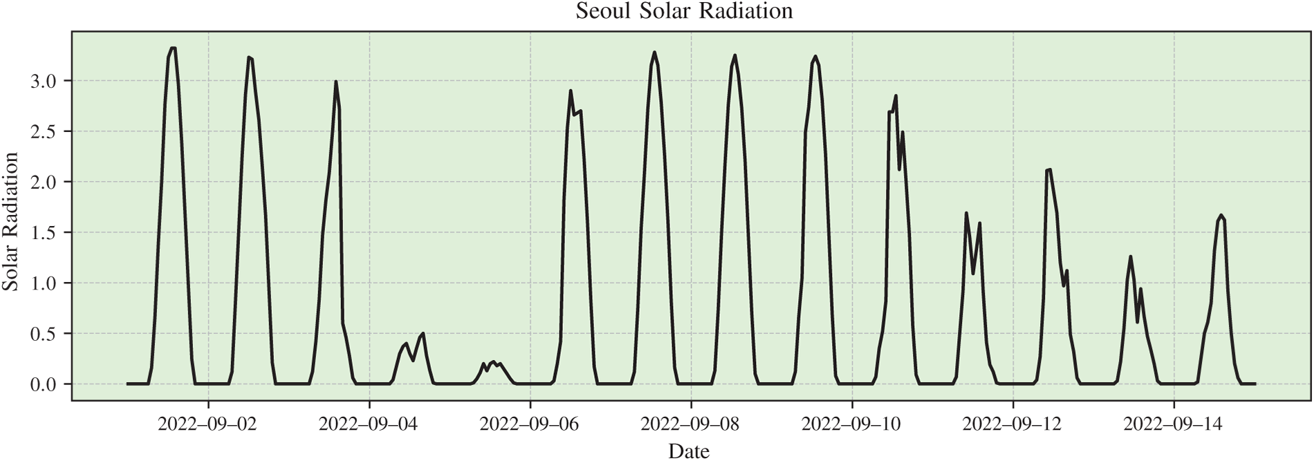
Figure 1: Example of solar irradiance time series observed in Seoul. Strong daily periodicity coexists with irregular fluctuations caused by weather conditions

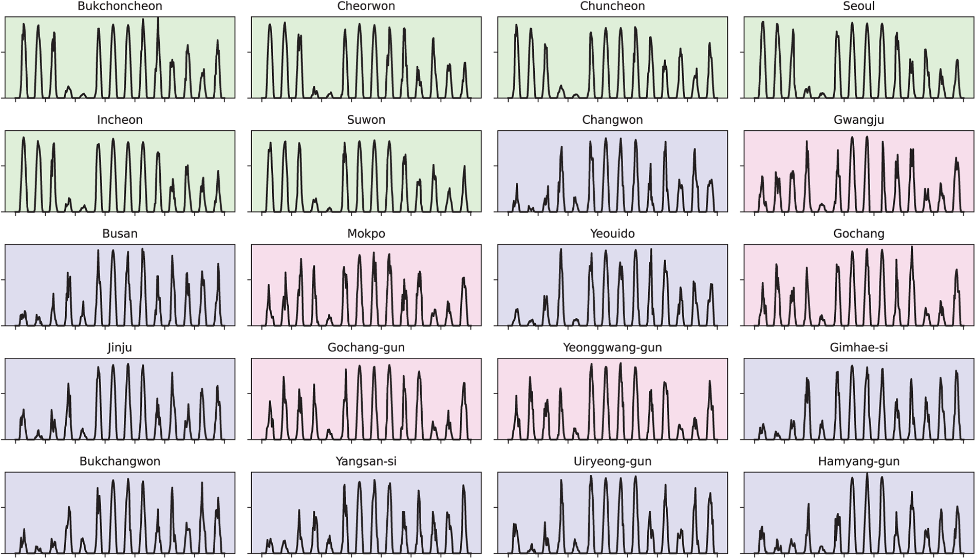
Figure 2: Solar irradiance time series observed simultaneously across multiple regions in Korea. Geographically closer locations exhibit higher similarity in their patterns

To capture such spatial interdependence, this study models each region as a node in a graph and infers inter-regional relationships from data within an STGNN framework. A key issue in STGNNs lies in how to define the connection strength between nodes. The most widely used approach is distance-based edge weighting, which is typically implemented in two ways. First, physical distances are mapped through a kernel function to compute continuous weights. For instance, Li et al. [16] employed an exponential mapping of distances in the DCRNN model, while setting connections beyond a certain distance to zero in order to ensure sparsity. Second, a threshold cutoff strategy is often applied, where nodes within a fixed radius are assigned a weight of 1 and all others are disconnected.

More recent studies have combined these two strategies. For example, DAGCRN [23] and DGCRN [24] employ Gaussian-based weights while applying a distance threshold to prune unnecessary connections. Similarly, research on dynamic graph learning generally assumes that the most common definition of a static adjacency matrix is distance-based, typically combining a Gaussian kernel with a cutoff [25,26].

Although distance-based approaches are simple and intuitive, and often effective when physical proximity is the dominant factor, they may be insufficient for real-world meteorological data. Geographic closeness does not always guarantee similar patterns. To illustrate this, we compared two regional pairs: Daejeon–Seosan and Cheorwon–Incheon (Fig. 3). Although both pairs are approximately 95 km apart, their irradiance patterns differ markedly. Daejeon–Seosan exhibit highly distinct fluctuations, whereas Cheorwon–Incheon show strong similarity.

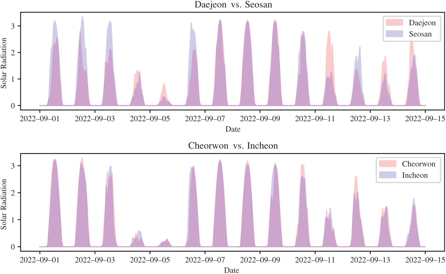
Figure 3: Comparison of solar irradiance patterns between Daejeon–Seosan (96.2 km) and Cheorwon–Incheon (94.9 km). Although the geographical distances are nearly identical, the irradiance variations differ substantially

This example clearly demonstrates that simple geographic distance alone cannot adequately explain the inter-regional relationships of solar irradiance. Factors such as topography, coastal vs. inland location, and elevation all exert significant influence on actual irradiance patterns. Therefore, in defining adjacency within STGNNs, it is important not to rely solely on distance-based approaches but to incorporate data-driven measures of similarity as well. In this way, regions that are geographically distant yet exhibit similar patterns can be strongly connected, while nearby regions with dissimilar patterns can be assigned weaker connections. In conclusion, this study aims to move beyond the limitations of purely distance-based methods and design an STGNN framework that integrates data-driven similarity into its structure.

2.2 Spurious Correlation in Periodic Data

The simplest way to quantify inter-node similarity is to compute correlation coefficients directly from the irradiance data.

Fig. 4 presents the correlation coefficients of solar irradiance across the country in matrix form. Most station pairs show very high correlation, and even the lowest case, between Seoul and Heuksando, is as high as 0.6422. However, these values are much higher than one would intuitively expect and do not always reflect actual climatological similarity.

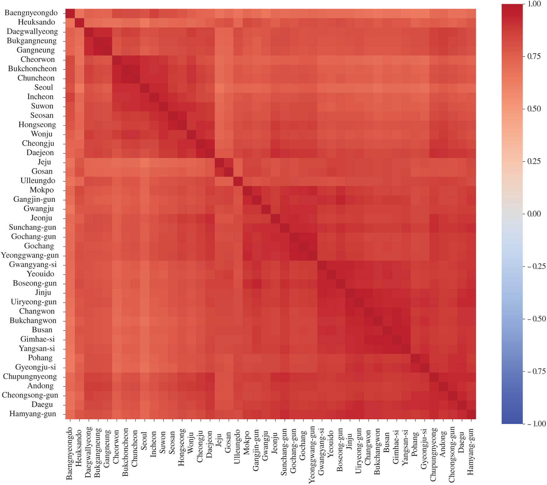
Figure 4: Correlation matrix of solar irradiance among all stations in Korea. Overall correlations are very high, with the lowest value observed between Seoul and Heuksando (0.6422)

Fig. 5 highlights this issue more clearly. Gochang–Yeonggwang shows a correlation of 0.9681, which aligns well with their highly similar time-series patterns. In contrast, Seoul–Heuksando has a correlation of 0.6422, yet their irradiance patterns often diverge. For example, when Seoul exhibits high irradiance, Heuksando often records near-zero values, and vice versa. Thus, correlation coefficients alone fail to capture true climatological similarity.

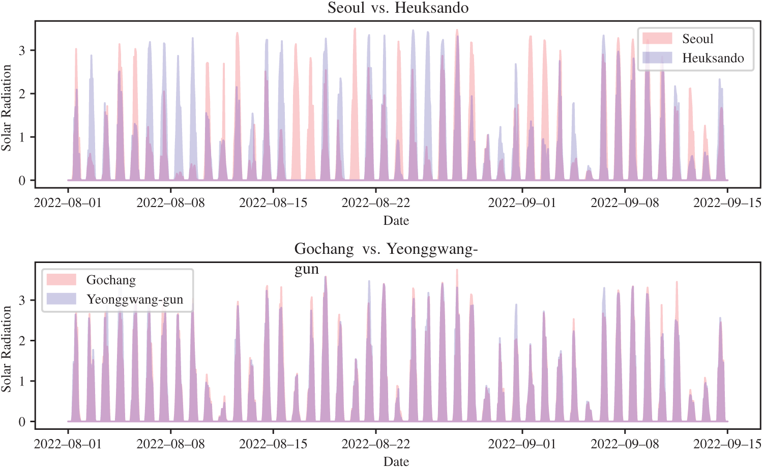
Figure 5: Comparison of solar irradiance time series: Seoul–Heuksando (top, correlation = 0.6422) and Gochang–Yeonggwang (bottom, correlation = 0.9681)

This illusion arises because both locations share strong daily periodicity: positive irradiance during the day and zero at night. Such recurring patterns artificially inflate correlation values, producing spurious correlations unrelated to actual climatic dependence. This issue is not unique to solar irradiance but commonly appears in other periodic time series such as temperature, precipitation, monthly retail sales, or weekday-driven trading volumes in stock markets. Consequently, relying solely on correlation coefficients in periodic data inherently leads to misinterpretation.

To further illustrate this point, we compare histograms of irradiance differences between Seoul–Heuksando and Gochang–Yeonggwang (Fig. 6).

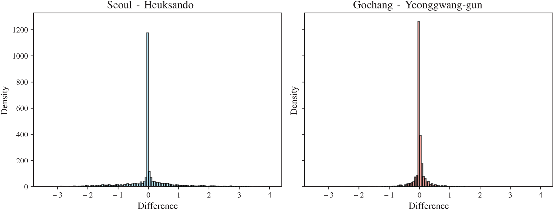
Figure 6: Histograms of irradiance differences for Seoul–Heuksando (left) and Gochang–Yeonggwang (right). Most values cluster around zero, but this mainly reflects nighttime periods when both sites record zero irradiance

Fig. 6 illustrates this phenomenon more intuitively. For both region pairs, the difference values are concentrated around zero, which superficially makes the time series appear highly similar. However, this outcome is mainly due to the periods after sunset, when both regions exhibit zero irradiance. In other words, the observed correlation does not stem from genuine climatic synchronization, but rather from a simple periodic structure that distorts the correlation.

Ultimately, for strongly periodic time series, simple correlation coefficients are insufficient to capture the true relationships between datasets. Some straightforward remedies include (i) excluding time points with zero irradiance, or (ii) removing nighttime periods when the sun has not risen. However, the former approach risks eliminating variations caused by clouds or precipitation, while the latter is difficult to apply uniformly due to seasonal and latitudinal differences.

In this study, we address these limitations by employing the EBT proposed by Choi and Oh [21,22]. EBT is designed to structurally separate the periodic component of a signal, enabling analysis of the residual variability. Beyond simple linear removal, it effectively eliminates spurious correlations caused by periodicity, thereby capturing the true spatial dependencies driven by actual climatic factors.

In the following section, we provide a detailed description of the definition and mathematical structure of EBT, and demonstrate how it can be used to decompose solar irradiance time series into amplitude modulation and periodic components. Based on this analysis, the core idea of the STGNN model proposed in this study is established.

3  Proposed Method

3.1 Multiplicative Decomposition of Time Series Signals

The solar irradiance time series yv,t can be modeled as the combination of two independent physical phenomena: one component representing the daily periodicity and the other capturing amplitude modulation due to weather conditions. Based on this observation, the irradiance signal at region v and time index t can be expressed as: yv,t=yv,tU×yv,tP where yv,tU denotes the amplitude modulation component, reflecting the daily maximum attainable irradiance influenced by weather conditions, and yv,tP denotes the periodic component, representing the normalized daily pattern (yv,tP∈[0,1]). This multiplicative decomposition follows the same signal modeling framework as the AM-demodulation introduced in Section 3.3 of Choi and Oh (2024) [22]. In the case of solar irradiance, the upper envelope corresponds to the maximum potential irradiance determined by cloud coverage and weather conditions, while the proportion captures the actual daily variation pattern, providing a clear physical interpretation.

3.2 Component Separation via Elastic Band Transform

The EBT is a decomposition technique specialized for signals with periodic structures. One of its key advantages is that it can effectively extract periodic components regardless of whether the signal follows a multiplicative or additive form. Consequently, EBT is highly advantageous in both physical and statistical signal analysis, as it enables the simultaneous identification of periodic patterns and their residual components [27].

Given a discrete signal yv={yv,t:t∈Z} and a multi-scale parameter τ, the ℓ-th elastic band is defined as yvℓ,τ={yv,tℓ,τ:yv,tℓ,τ=svℓ,τ(t), t∈Z},ℓ=1,…,τ, where svℓ,τ(⋅) is an interpolation function constructed from the points {…,yv,ℓ−τ,yv,ℓ,yv,ℓ+τ,…}. In this study, we adopt linear interpolation for simplicity. An elastic band thus connects signal values with the same phase at intervals of τ, and the collection of τ elastic bands fully represents all phases of the signal.

EBT is originally designed as a multiscale method that utilizes various statistics computed from multiple bands, such as the mean, variance, and the rates of change of these quantities. However, in this study, we specifically focus on the maximum value across bands at each time point, since the analysis of solar irradiance is particularly concerned with the daily maximum attainable irradiance. By constructing elastic bands and then taking their pointwise maximum, we effectively estimate the upper envelope of the signal, which directly serves as yv,tU.

The upper envelope is defined as the maximum across the τ elastic bands at each index t: uv,tyv,τ=maxℓ∈{1,…,τ}yv,tℓ,τ.

Accordingly, in the volume-based EBT framework, it can be expressed as uvyv,τ={uv,tyv,τ:t∈Z}.

In this study, we set τ=24 to explicitly capture the daily periodicity. This choice means that each elastic band connects information every 24 time steps, corresponding to a one-day interval. By observing the signal with a daily step size, the method can clearly capture the daily periodic effect while simultaneously enabling the separation of the residual component with the periodic effect removed.

Once the upper envelope is estimated, the original signal can be naturally decomposed into an amplitude modulation component and a periodic component. The amplitude modulation component is defined as the upper envelope itself, yv,tU=uv,tyv,τ which represents the maximum possible irradiance achievable at location v and time t. The periodic component is then obtained by normalizing the original signal with the amplitude component, yv,tP=yv,tyv,tU+ε where ϵ=10−10 is a small numerical constant introduced to prevent the denominator from approaching zero.

As a result, the EBT-based demodulation decomposes yv,t into two interpretable components. The term yv,tU serves as the envelope component that reflects the influence of weather conditions, while yv,tP represents the normalized pattern component that captures the daily periodicity. This decomposition enables a physically meaningful interpretation of signals where periodicity and amplitude modulation are multiplicatively combined.

Fig. 7 illustrates the process of applying EBT to solar irradiance time series data from Seoul over a two-week period (September 1–15, 2022). The left panels demonstrate the construction of elastic bands and the extraction of the upper envelope. With the period parameter set to τ=24, we construct 24 distinct elastic bands yvℓ,τ for ℓ=1,…,24, where each band ℓ connects signal values occurring at the same hour of the day through linear interpolation (e.g., band 1 connects all 1:00 AM values, band 2 connects all 2:00 AM values, and so forth). These 24 elastic bands, shown as thin gray curves in the left panels, collectively encompass all possible phases within a 24-h cycle. At each time point t, the upper envelope uv,tyv,τ is computed as the pointwise maximum across all elastic bands, depicted as the bold red curve overlaying the gray elastic bands in the left panels.

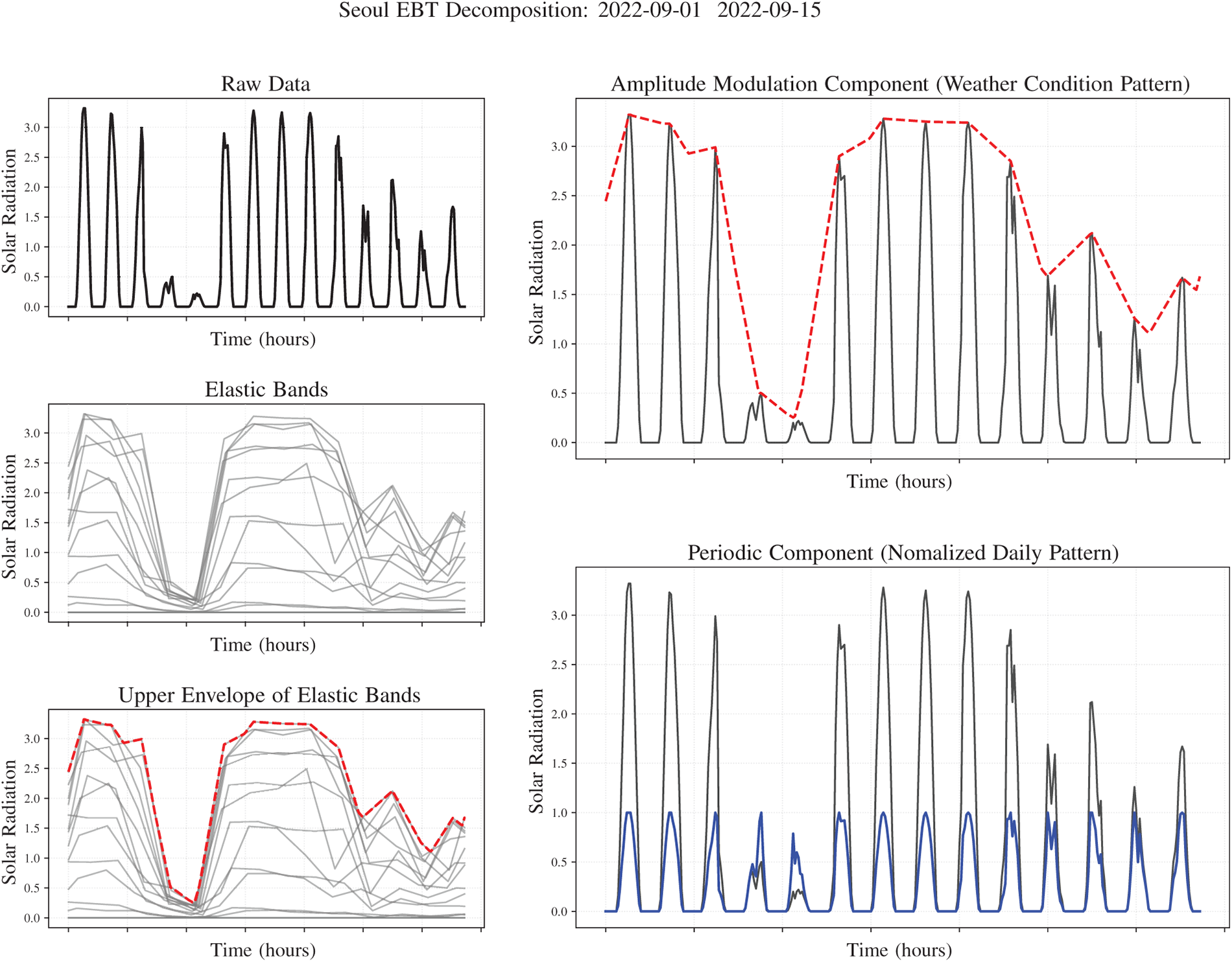
Figure 7: Illustration of the EBT decomposition process for solar irradiance time series. Left: Construction of elastic bands with τ=24 and extraction of the upper envelope (red curve) as the maximum across all bands at each time point. Right: Decomposed components showing the amplitude modulation component yv,tU (top) and the normalized periodic component yv,tP (bottom)

The right panels show the components decomposed by EBT. The upper panel displays the amplitude modulation component yv,tU (red curve), which represents the upper envelope capturing weather-driven variations in maximum achievable irradiance. Clear days (e.g., days 3 and 6) exhibit high and smooth curves, while cloudy or rainy days (e.g., days 4 and 5) show significantly lower and irregular patterns. The lower panel presents the periodic component yv,tP (blue curve), which represents the pure daily pattern with weather effects removed. This component takes values between 0 and 1, revealing the geometric pattern based on solar elevation. It maintains a consistent bell-shaped pattern every day regardless of weather conditions, as the daily cycle is determined by geographic location (latitude and longitude). EBT separates the predictable geometric pattern (yv,tP) from the stochastic weather-driven variations (yv,tU). This enables independent modeling of each component with separate graph structures, addressing the spurious correlation problem discussed in Section 2.2.

A critical distinction of EBT is that it assumes a multiplicative decomposition model (yv,t=yv,tU×yv,tP), unlike conventional decomposition methods such as Empirical Mode Decomposition (EMD) [28], Seasonal-Trend decomposition using Loess (STL) [29], and Wavelet decomposition [30], which assume additive models. This multiplicative framework is particularly well-suited for solar irradiance data, where the amplitude of the daily pattern is modulated by weather conditions rather than being added as an independent component. For readers interested in understanding why EBT is specifically required for this application and how it compares empirically to these alternative methods, we refer to Appendix A, which provides a detailed comparison and justification.

3.3 Spatial Correlation Analysis of Decomposed Components

For N=44 regions, the spatial correlations of the decomposed components are computed independently. The correlation matrix of the periodic component is defined as rv,sP=∑t=1T(yv,tP−y¯vP)(ys,tP−y¯sP)∑t=1T(yv,tP−y¯vP)2∑t=1T(ys,tP−y¯sP)2, where y¯vP=1T∑t=1Tyv,tP. Since the periodic component is largely determined by geographic location (e.g., longitude), most region pairs yield values close to rv,sP≈1. The correlation matrix of the amplitude modulation component is calculated as rv,sU=∑t=1T(yv,tU−y¯vU)(ys,tU−y¯sU)∑t=1T(yv,tU−y¯vU)2∑t=1T(ys,tU−y¯sU)2, where y¯vU=1T∑t=1Tyv,tU. The amplitude modulation component reflects regional climatic characteristics such as topography and maritime climate. Importantly, since the periodicity is removed, rv,sU captures only the true climatological similarity between regions.

Fig. 8 illustrates the spatial correlation structure of EBT-decomposed components, revealing three key advantages of the decomposition. First, the spurious correlation induced by the daily periodic pattern in the raw data (rv,s) is effectively eliminated in the amplitude modulation component (rv,sU). While the raw data exhibits uniformly high correlations across nearly all region pairs due to the shared daily cycle, the amplitude modulation component shows a clear block structure where only geographically proximate or climatologically similar regions maintain strong correlations. This removal of spurious correlations enables the model to capture genuine weather-driven spatial dependencies.

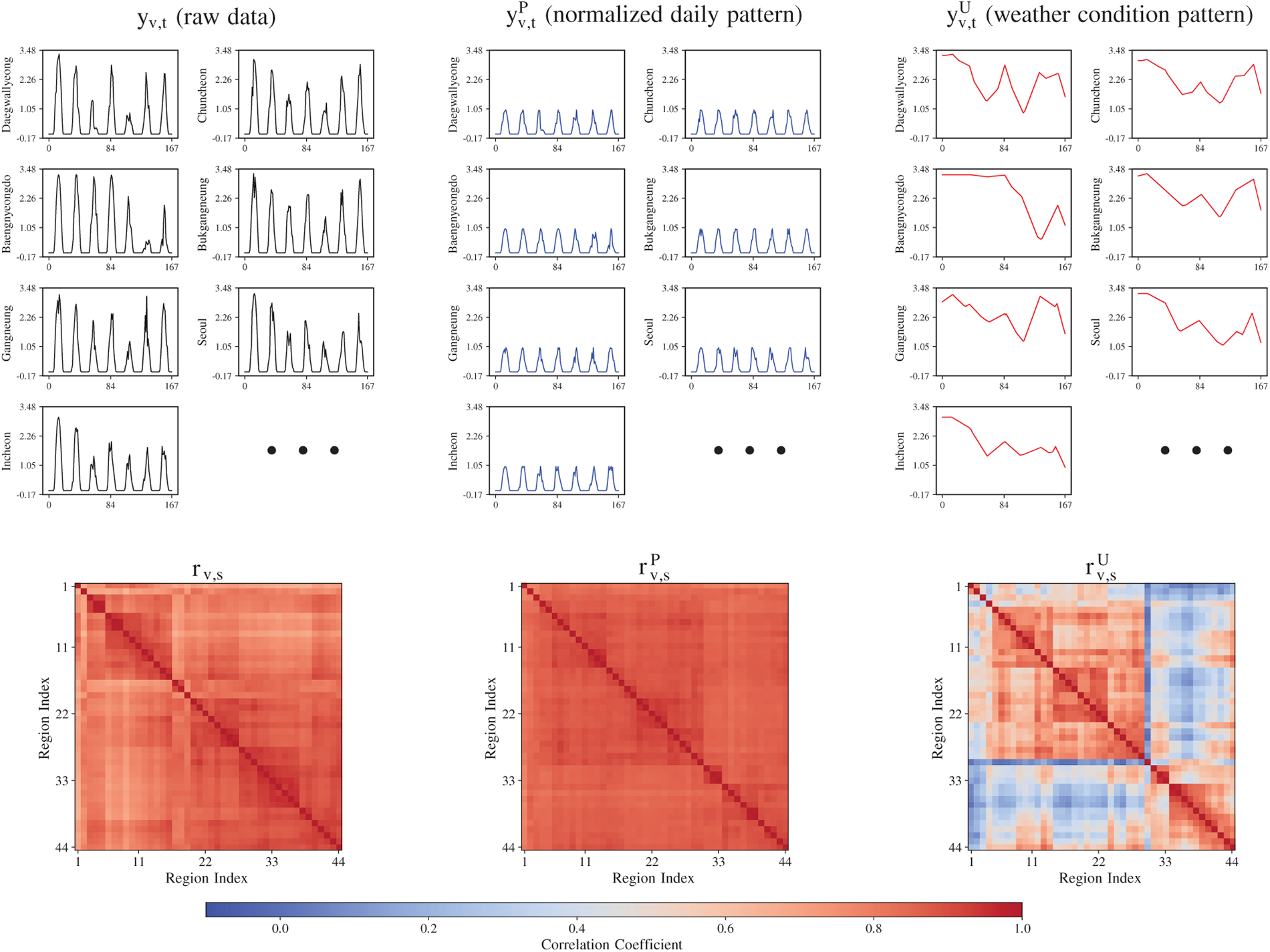
Figure 8: Spatial correlation structure of EBT-decomposed components. Top: Sample time series of yv,t, yv,tP, and yv,tU from seven regions. Bottom: Correlation matrices across 44 regions showing uniform high correlations for the periodic component (rv,sP) and structured regional clustering for the amplitude modulation component (rv,sU)

Second, the decomposition produces highly interpretable components with distinct temporal characteristics. The periodic component yv,tP exhibits regular bell-shaped patterns bounded between 0 and 1, representing the pure geometric pattern of solar elevation. All regions share nearly identical patterns (rv,sP≈1), making this component highly predictable. In contrast, the amplitude modulation component yv,tU captures weather-driven variations with a notably simple temporal structure—the complete removal of periodicity results in smooth, slowly-varying patterns. This simplicity has important implications for forecasting: modeling yv,tU requires relatively few temporal lags and does not necessitate complex filter architectures, as the temporal dependencies are substantially less intricate than those in the raw data.

Third, the decomposition naturally leads to a dual-graph structure where spatial connectivity is defined differently for each component. For predicting yv,tP, a dense graph structure is appropriate since nearly all regions exhibit high correlations (rv,sP≈1). This is reasonable because the daily pattern is determined solely by geographic location (latitude and longitude) and is independent of weather conditions, thus all regions share similar patterns. Conversely, for predicting yv,tU, a sparse graph structure is more suitable as the correlation matrix exhibits clear block structure. This sparsity reflects the fact that weather conditions vary significantly across regions, with strong dependencies existing only among geographically adjacent or climatologically similar areas. This component-specific graph design enables more accurate representation of the underlying spatial dependencies and improves forecasting performance.

Construction of Spatio-Temporal Graph Neural Networks

In this study, the periodic and amplitude modulation components of solar irradiance are modeled independently by constructing separate graphs for each component. A graph is defined as 𝒢k=(𝒱,ℰ,Ak), where k∈{P,U}. Here, 𝒱={v1,…,vN} denotes the set of N=44 nodes corresponding to observation sites, ℰ is the set of edges, and Ak∈RN×N is the adjacency matrix with entries Av,sk=rv,sk. At time index t, the graph signal is expressed as xtk=[y1,tk,y2,tk,…,yN,tk]T∈RN.

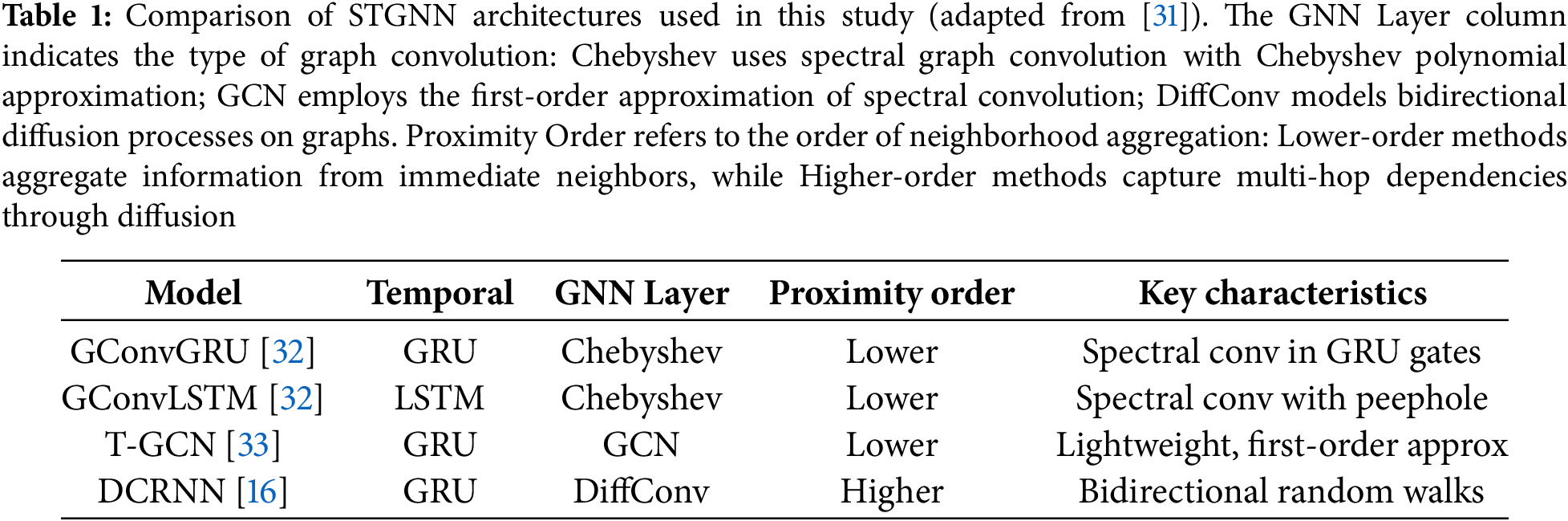
Based on this graph representation, four representative Spatio-Temporal Graph Neural Network (STGNN) architectures are employed to effectively capture spatio-temporal dependencies. Among them, the Graph Convolutional Gated Recurrent Unit (GConvGRU) [31], the Graph Convolutional Long Short-Term Memory (GConvLSTM) [32], and the Temporal Graph Convolutional Network (T-GCN) [33] share the common feature of defining graph convolution in the spectral domain, while differing in how temporal dependencies are incorporated.

Graph convolution is defined in the spectral domain as follows: gθ⋆x=Ugθ(Λ)UTx, where x∈RN is a graph signal represented as a vector of values over N nodes. U denotes the eigenvector matrix of the normalized graph Laplacian L~=I−D−1/2AD−1/2, and Λ is the corresponding diagonal matrix of eigenvalues. Thus, U and Λ serve as the basis and the frequencies of the graph Fourier transform, respectively. The function gθ(⋅) is a spectral filter defined by the set of learnable parameters θ={θ0,θ1,…}. In other words, gθ operates on the eigenvalues (graph frequencies) to determine how each frequency component is modulated. Intuitively, this definition can be understood as: (i) transforming the graph signal x into the Fourier domain via UTx, (ii) filtering the spectral coefficients through gθ(Λ), and (iii) applying the inverse transform with U to map the result back to the graph domain. Since direct eigendecomposition is computationally expensive, it is common to approximate gθ(⋅) using Chebyshev polynomials. This allows the convolution to capture higher-order neighborhood information efficiently without explicitly computing the eigenbasis.

Building on this foundation, the GConvGRU replaces the linear transformations of a standard GRU with graph convolutions, thereby incorporating spatial structure into the state update process [31]. The GConvLSTM extends the gating operations of the LSTM with graph convolutions to capture long-term dependencies more effectively, making it well suited for modeling the irregular amplitude modulation component [32]. Furthermore, the T-GCN proposed by Zhao et al. [33] combines GCN and GRU in a lightweight framework, jointly modeling spatial dependencies and temporal dynamics while maintaining computational efficiency.

Meanwhile, Li et al. [16] proposed the Diffusion Convolutional Recurrent Neural Network (DCRNN), which introduces diffusion convolution in place of the traditional spectral-based graph convolution. This approach models graph diffusion processes that account for both directionality and edge weights, and the diffusion convolution is formally defined as follows: x(j+1)=∑m=0M−1(θm,1(DO−1A)m + θm,2(DI−1AT)m)x(j).

Here, j denotes the layer index of the network, and x(j)∈RN represents the graph signal at layer j, which is a vector of feature values corresponding to N nodes (regions). The matrices DO and DI are the out-degree and in-degree diagonal matrices, respectively, defined as the row and column sums of the adjacency matrix. The parameters θm,1 and θm,2 are learnable coefficients that control the contributions of forward and backward m-hop diffusions. In other words, this operation jointly incorporates information propagated up to m hops in both forward and reverse directions, while allowing the network to learn different weights for each hop. Through this formulation, DCRNN effectively models spatial diffusion processes with directionality and asymmetry, and by integrating it with the GRU structure, it further captures temporal dynamics to represent complex and nonlinear spatio-temporal dependencies.

In summary, this study applies and compares four models—GConvGRU, GConvLSTM, T-GCN, and DCRNN—within a unified framework, thereby verifying the generality and robustness of the proposed decomposition–prediction approach from multiple perspectives. Table 1 summarizes the key architectural differences among these four STGNN models.

3.4 Component-Specific Optimization and Final Prediction

The key advantage of the proposed approach is that it enables independent model designs tailored to the characteristics of each component. For the periodic component, strong inter-regional correlations (ρrsP≈1) allow the use of information from all regions, and simple repetitive patterns can be effectively captured with relatively straightforward models.

In contrast, the amplitude modulation component leverages selective regional information based on climatic similarity, requiring more filters and sophisticated architectures to capture complex meteorological variations. This ensures that each component is optimized according to its inherent characteristics.

Finally, at prediction horizon t+h, the forecast is obtained by recombining the predictions of the two components: y^v,t+h=y^v,t+hU×y^v,t+hP, where y^v,t+hU and y^v,t+hP denote the outputs of independently trained models for the amplitude modulation and periodic components, respectively. This decomposition-recombination strategy enables the model to capture both periodic structures and aperiodic fluctuations, thereby enhancing both predictive accuracy and interpretability.

Fig. 9 illustrates the overall architecture of the proposed forecasting framework. The input time series is decomposed into a periodic component and an amplitude modulation component via the EBT. Each component is then processed by an independent STGNN model. The outputs of these models are subsequently recombined through a multiplicative operation to produce the final forecast. This design not only disentangles periodic patterns from irregular fluctuations but also improves the model’s generalization capability and interpretability.

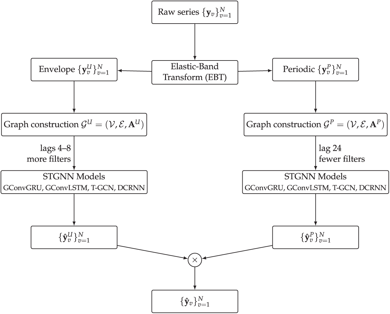
Figure 9: Process of decomposing the raw time series into a periodic component and an amplitude modulation component using the EBT, constructing separate graphs 𝒢P and 𝒢U, applying STGNN-based models (GConvGRU, GConvLSTM, T-GCN, DCRNN) to each component independently, and recombining the two prediction results to obtain the final forecast

4  Experiments and Comparisons

4.1 Experimental Setup

The experimental dataset consists of hourly solar irradiance measurements from 44 regions, totaling 2568 time steps (approximately 107 days). The training period covers 80% of the data (2054 time steps, about 85.6 days), while the remaining 20% (514 time steps, about 21.4 days) is used for testing. Notably, the test set includes the early September 2022 period when the Korean Peninsula was struck by the super typhoon Hinnamnor. This event is recorded as one of the most powerful typhoons to directly impact the region, with peak wind speeds reaching 40–50 m/s and accompanied by torrential rainfall. As a result, solar irradiance exhibited extreme fluctuations, with some locations experiencing nearly zero values for several consecutive days. The inclusion of this period provides a critical opportunity to evaluate whether the proposed model can remain stable under extreme weather conditions. All experiments were implemented using PyTorch and the PyTorch Geometric Temporal library [31].

The predictive performance of the models was evaluated using a variety of metrics, including MAE, MSE, RMSE, R2, MAPE, and MASE. In this section, we primarily focus on the MSE results for consistency in analysis. However, additional metrics were also computed, and their results are presented in Appendix A to verify that the trends observed in the main text are consistently reflected across different evaluation measures.

For empirical validation, four representative STGNN models—GConvGRU, GConvLSTM, T-GCN, and DCRNN—are examined. For each model, the temporal dependency length (lags) and the number of convolutional filters are systematically varied to investigate their effect on predictive performance. This experimental design allows not only architectural comparison but also analysis of model behavior under different receptive fields and capacities.

4.2 Performance Comparison

As demonstrated in Fig. 8, the amplitude modulation component yv,tU exhibits a notably simple temporal structure. The complete removal of periodicity results in smooth, slowly-varying patterns that are substantially less complex than those in the raw data. This observation has important implications for model design: yv,tU requires relatively few temporal lags, as the temporal dependencies are much simpler than in the original time series. In contrast, the periodic component yv,tP represents the geometric pattern of solar elevation and may benefit from considering a longer history to capture its regular structure.

Based on this insight, we propose an asymmetric lag configuration where the amplitude modulation component is modeled with a short lag (specifically, lag = 4), while the periodic component can utilize a longer lag when needed. This design choice is motivated by the distinct temporal characteristics of each component and aims to balance model complexity with predictive accuracy.

In this section, we systematically compare three forecasting strategies across four representative STGNN architectures (GConvGRU, GConvLSTM, T-GCN, and DCRNN):

•   Classic: The conventional approach that directly feeds the entire time series yv,t into a single STGNN with lag L.

•   Proposed (L,L): A baseline decomposition approach where both yv,tP and yv,tU are modeled with identical lag L. The final prediction is obtained by multiplying the two component predictions.

•   Proposed (4,L): The proposed asymmetric configuration where yv,tU uses lag 4 and yv,tP uses lag L. This reflects the empirical finding that the amplitude component requires fewer temporal dependencies.

For each STGNN model, we vary both the lag length (L∈{8,12,24}) and the number of convolutional filters (F∈{8,16,24,32}) to systematically investigate their effects on predictive performance under different model capacities and receptive field sizes.

Table 2 presents a comprehensive comparison of the three forecasting strategies across four STGNN models. All results are reported as mean ± standard deviation over 10 independent runs with different random initializations, demonstrating the reproducibility of our findings. The results demonstrate a clear pattern: the Proposed (4,L) configuration consistently outperforms both the Classic and Proposed (L,L) approaches across most hyperparameter settings. This validates our hypothesis that the amplitude modulation component yv,tU, due to its simple temporal structure, requires only short-term temporal dependencies for accurate forecasting.

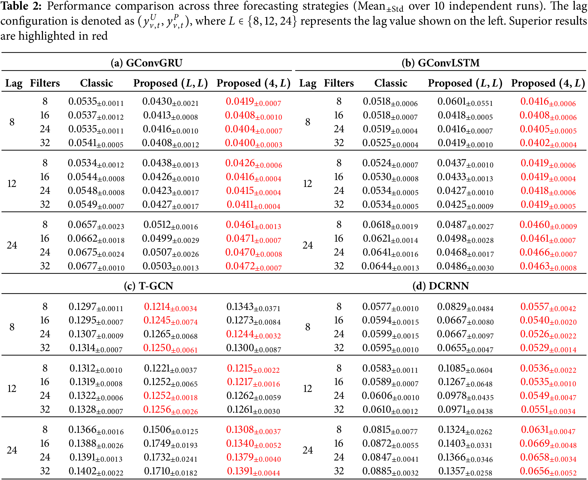
Superior Performance of GConvGRU and GConvLSTM.

Among the four STGNN architectures tested, GConvGRU and GConvLSTM demonstrated substantially superior performance compared to DCRNN and T-GCN. GConvGRU achieved the best overall performance with an MSE of 0.0400±0.0003 (lag (4,8), 32 filters), while GConvLSTM obtained a nearly identical MSE of 0.0402±0.0004 with the same configuration. Remarkably, both models exhibit exceptionally low standard deviations (<0.0005), indicating highly stable and reproducible performance across multiple runs. In contrast, DCRNN achieved a best MSE of 0.0526±0.0022 and T-GCN reached 0.1215±0.0022—both significantly higher than the gate-based models.

The superior performance of GConvGRU and GConvLSTM can be attributed to their gating mechanisms, which are particularly well-suited to learning from decomposed components with distinct temporal characteristics. The gate structures enable these models to adaptively control information flow, selectively retaining relevant patterns from the periodic component yv,tP while filtering out noise from the amplitude modulation component yv,tU. Furthermore, both models show consistent improvements with the Proposed (4,L) strategy across all lag and filter configurations (Table 2a,b), with no instances of performance reversal. This robustness highlights the compatibility between the component-wise decomposition framework and gate-based recurrent architectures, making GConvGRU and GConvLSTM the recommended choices for solar irradiance forecasting with EBT decomposition.

Effect of Asymmetric Lag Configuration.

The comparison between Proposed (L,L) and Proposed (4,L) reveals the value of component-specific lag tuning. For example, in GConvGRU with lag 24 and 24 filters, the Classic approach yielded an MSE of 0.0675±0.0024, while Proposed (L,L) improved this to 0.0507±0.0026. However, Proposed (4,L) further reduced the error to 0.0470±0.0008—a gain of more than 30% compared to Classic and an additional 7% improvement over Proposed (L,L). Importantly, Proposed (4,L) also exhibits significantly lower variance (std = 0.0008) compared to both Classic (std = 0.0024) and Proposed (L,L) (std = 0.0026), indicating more stable optimization. Similar trends are observed across GConvLSTM and other models, demonstrating that shortening the lag for yv,tU consistently enhances both predictive accuracy and training stability.

Resolution of Performance Reversal in DCRNN.

A particularly noteworthy finding emerges from the DCRNN results. In several configurations, the Proposed (L,L) approach underperformed relative to Classic, exhibiting a performance reversal. For instance, under lag 12 with 24 filters, Classic achieved an MSE of 0.0606±0.0010, while Proposed (L,L) degraded to 0.0978±0.0435—note the extremely large standard deviation, indicating highly unstable training. However, when the lag for yv,tU was reduced to 4, this reversal disappeared entirely: Proposed (4,L) achieved an MSE of 0.0549±0.0047, significantly surpassing both Classic and Proposed (L,L), with much more stable performance. This behavior can be attributed to the inherently short-term nature of the amplitude component. Using longer lags for yv,tU appears to introduce noise and irrelevant temporal information, which degrades both performance and training stability. By contrast, the asymmetric lag strategy effectively captures the essential dynamics of yv,tU without overfitting to spurious patterns.

Effect of Filter Size.

The effect of filter size varies across models but generally follows a consistent pattern. Performance improves as the number of filters increases from 8 to 16 or 24, reflecting the model’s ability to capture richer spatial dependencies. However, further increasing the filter size to 32 often yields diminishing returns or even slight degradation, particularly in models with longer lags. This suggests a risk of overfitting when model capacity becomes excessively large relative to the available training data.

T-GCN Performance Characteristics.

T-GCN exhibits a distinct behavior compared to other models. While the Proposed (4,L) configuration shows mixed results, T-GCN’s absolute MSE values are notably higher (around 0.12–0.14) than those of GConvGRU, GConvLSTM, and DCRNN (around 0.04–0.08). Interestingly, with smaller lag values (8 and 12), the Proposed (L,L) strategy often outperforms Proposed (4,L). For example, with lag 8 and 8 filters, Proposed (L,L) achieves an MSE of 0.1214±0.0034, while Proposed (4,L) yields 0.1343±0.0371 (compared to Classic’s 0.1297±0.0011). Notably, Proposed (4,L) shows much higher variance in this configuration (std = 0.0371), suggesting training instability. However, with larger lag (24), the pattern reverses: Proposed (4,L) consistently outperforms both Classic and Proposed (L,L), with more stable performance. This may indicate that T-GCN’s architecture interacts differently with the decomposed components, possibly requiring longer context for the periodic component to fully benefit from the asymmetric configuration.

Statistical Significance.

To verify the statistical significance of these improvements, we conducted Diebold-Mariano tests [34] comparing Classic and Proposed (L,L) methods across all 48 configurations (4 models × 3 lags × 4 filters). The results demonstrate overwhelming significance: 47 out of 48 configurations (97.9%) achieved p<0.01, with median p-value <10−6. GConvGRU showed the strongest evidence (average DM statistic: 21.26, improvement: 25.25%), followed by GConvLSTM (19.53, 23.14%), DCRNN (13.84, 16.55%), and T-GCN (5.88, 4.33%). The single non-significant case occurred in T-GCN with lag 8 and 8 filters, consistent with its distinct short-lag behavior noted earlier. This near-universal statistical significance confirms that the observed improvements reflect genuine advantages rather than random variation.

Comparison with Non-Spatial Baselines.

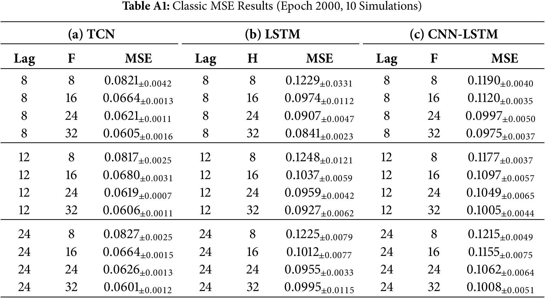
To contextualize the STGNN results, we also evaluated conventional non-spatial architectures—Temporal Convolutional Network (TCN) [14], Long Short-Term Memory (LSTM) [12], and CNN-LSTM hybrid [13]—under extended training (2000 epochs). Appendix B presents comprehensive results across 36 configurations. The best non-spatial model, TCN with lag 24 and 32 filters, achieves MSE = 0.0601±0.0012—substantially worse than not only the Proposed STGNNs (MSE ≈0.040) but also the Classic STGNN baselines (MSE ≈0.053 for GConvGRU). This performance gap confirms that spatial correlation modeling through graph structures is essential for multi-site solar radiation forecasting.

Summary.

The Proposed (4,L) configuration consistently outperforms Classic across STGNN architectures, with GConvGRU and GConvLSTM achieving the best performance (MSE ≈0.040). The results validate that EBT decomposition enables component-specific modeling strategies, with yv,tU requiring only short lags while yv,tP benefits from longer contexts.

4.3 Case Study: Performance during Typhoon Hinnamnor

To evaluate model robustness under extreme weather conditions, we analyzed performance during Super Typhoon Hinnamnor, which struck the Korean Peninsula on September 4–6, 2022. This typhoon reached peak intensity with 920 hPa central pressure and maximum winds of 105 knots, bringing torrential rainfall exceeding 300 mm and causing near-zero solar irradiance across many regions [35]. We compared the Classic approach against the best-performing Proposed (4,4) configuration (GConvGRU with 16 filters) during the extended typhoon period (August 30–September 8, 2022).

Table 3 shows the top 9 regions ranked by improvement rate: Improvement(%)=(MSEClassic−MSEProposed)/MSEClassic×100. The proposed method achieved a 33%–45% reduction in MSE in these regions, with Gyeongju-si showing the largest improvement (44.9%, from 0.0791 to 0.0436). All nine of the top regions are concentrated in southeastern Korea, directly in the typhoon’s path (see [35] for the detailed typhoon track).

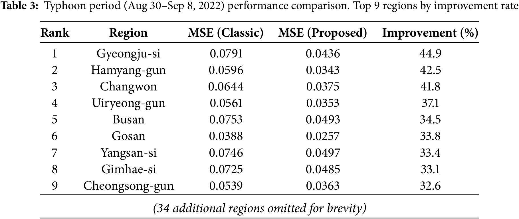
Fig. 10 shows the geographic distribution of the top 9 regions with highest improvement rates (left) and their solar irradiance time series before and after the typhoon (right). The shaded area indicates the typhoon-affected period. During this period, the proposed method significantly reduces peak overestimation compared to the Classic method, demonstrating marked performance improvement. These results show that the proposed method effectively adapts to rapid climate changes. This can be attributed to the separate and independent modeling of daily periodic patterns and weather-driven amplitude variations, enabling more accurate capture of abrupt meteorological changes.

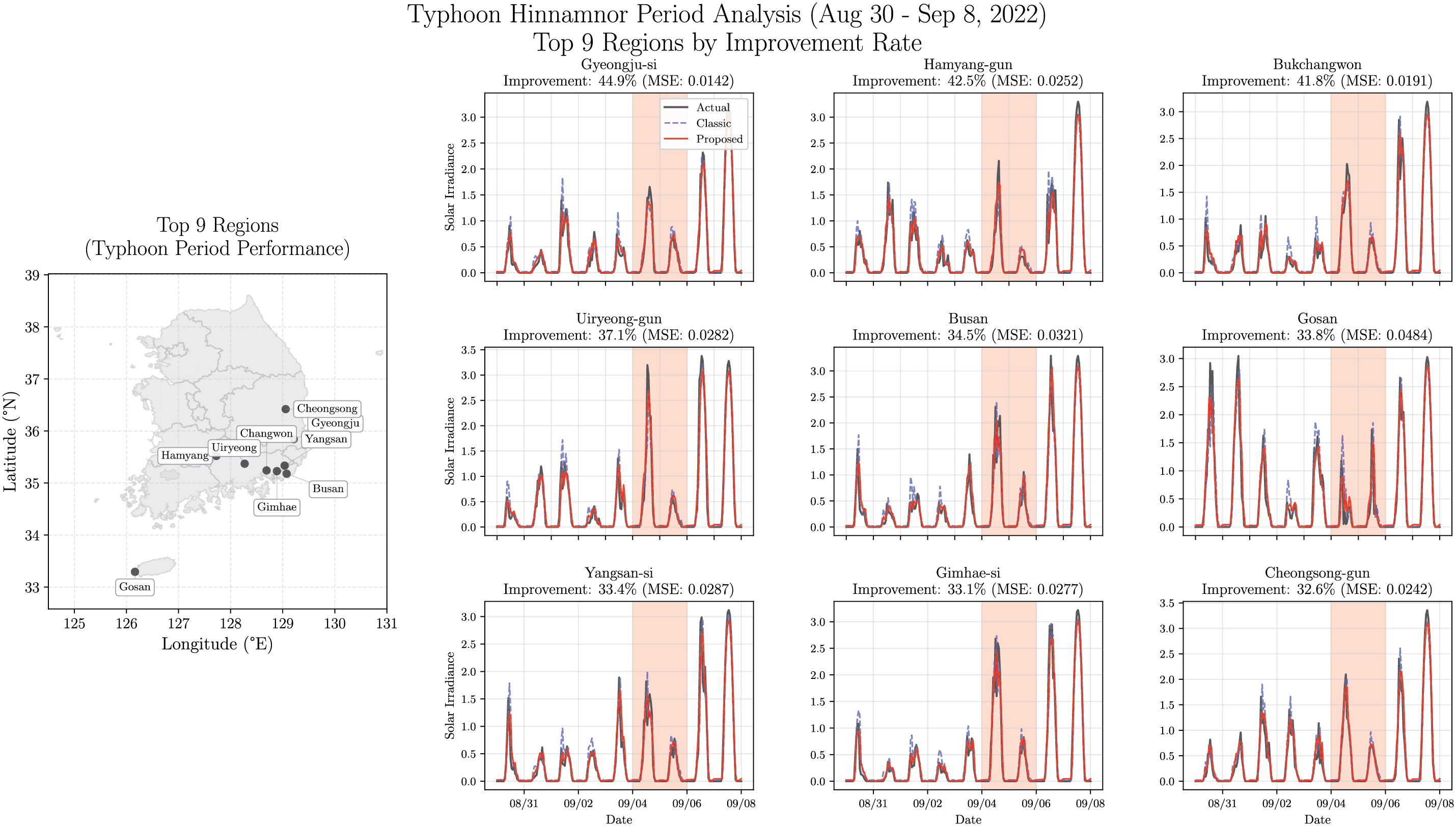
Figure 10: Top 9 regions by typhoon period improvement rate. Left: Geographical distribution. Right: Time series comparison during Typhoon Hinnamnor (Aug 30–Sep 8, 2022). Red shading indicates core impact period (Sep 4–6)

This case study demonstrates that the decomposition-based framework provides substantial benefits during extreme weather events—precisely when accurate forecasts are most critical for grid management. By explicitly separating periodic astronomical patterns from meteorologically-driven amplitude variations, the proposed approach better captures rapid transitions between extreme suppression and recovery. The consistent 32–45% improvement across diverse regions suggests that this framework offers practical operational advantages for solar forecasting in typhoon-prone areas.

5  Conclusion

This study goes beyond developing a high-performing forecasting model—it proposes a novel analytical framework for solar radiation data that reveals several fundamental insights applicable beyond the specific implementation details. While we employed the EBT and STGNNs in this work, the core findings suggest broader principles for renewable energy forecasting that transcend these particular methodological choices.

Multiplicative Decomposition as a Fundamental Principle.

Our first key insight is that solar radiation should be decomposed using a multiplicative model that separates daily periodic patterns from meteorological amplitude variations. This decomposition principle holds value regardless of the specific decomposition technique employed—whether EBT, or other methods. The fundamental advantage lies in mitigating spurious correlations that arise when periodic astronomical patterns interact with irregular meteorological variability in additive frameworks. By treating these components as multiplicative factors, we enable models to learn genuine causal relationships rather than artifacts of periodicity-induced correlations. This finding challenges the conventional practice of treating solar forecasting as a univariate or multivariate time series problem without explicit consideration of the multiplicative nature of underlying physical processes.

Distinct Graph Structures for Different Physical Processes.

The second critical insight concerns the inherently different spatial correlation structures exhibited by daily patterns vs. meteorological patterns when represented as graph signals. Daily periodic patterns, governed by astronomical factors such as latitude, longitude, and solar elevation, exhibit broad regional similarities. Regions sharing similar astronomical characteristics form cohesive clusters, resulting in a relatively dense graph structure where many nodes are strongly connected. In contrast, meteorological amplitude patterns are driven by localized weather phenomena—cloud formations, atmospheric circulation, and terrain effects—that create sparser spatial dependencies. Only geographically proximate regions or those sharing similar microclimatic conditions exhibit strong correlations. This sparsity is particularly advantageous for graph neural networks, which are specifically designed to leverage sparse connectivity for efficient and effective learning. Consequently, while daily patterns may benefit from alternative modeling approaches, meteorological patterns are especially well-suited to graph-based representation and learning.

Component-Specific Modeling Strategies.

Third, we observe that the optimal forecasting strategy differs fundamentally between the two decomposed components. The periodic component yv,tP, characterized by strong regularity and seasonal variations (due to changing sunrise/sunset times), may not require complex data-driven models at all. Instead, physics-based models or astronomically-informed parametric approaches could provide more robust and interpretable predictions. Indeed, in operational settings, one might consider replacing learned models for yv,tP with deterministic astronomical calculations, reserving machine learning capacity exclusively for the stochastic amplitude component. Conversely, the amplitude modulation component yv,tU, which lacks periodicity and exhibits simpler temporal dynamics, is ideally suited for graph signal processing. Its sparse spatial structure and irregular temporal patterns align well with STGNN architectures. Furthermore, this component presents a natural integration point for external meteorological data—satellite imagery, numerical weather prediction outputs, or real-time atmospheric measurements—which could substantially enhance forecasting accuracy in future extensions.

Implications for Solar Forecasting Practice.

These insights collectively suggest that effective solar radiation forecasting should not be approached as a monolithic spatio-temporal prediction task. Rather, practitioners should:

1.    Explicitly separate periodic astronomical influences from meteorologically-driven variability using multiplicative decomposition.

2.    Recognize that the resulting components exhibit fundamentally different spatial correlation structures, with meteorological patterns being particularly amenable to graph-based modeling.

3.    Adopt component-specific modeling strategies: deterministic or physics-based methods for periodic patterns, and data-driven graph neural networks for amplitude variations.

4.    Leverage external meteorological data specifically for the amplitude component, where weather-related information is most relevant.

Beyond the specific performance improvements demonstrated in this work (25% MSE reduction with GConvGRU, robust performance under extreme typhoon conditions), these principles offer a conceptual framework that can guide future research in solar and potentially other renewable energy forecasting domains.

Limitations and Future Directions.

Despite the promising results, this study has several limitations. First, the proposed framework relies solely on historical solar radiation data without incorporating exogenous variables such as satellite cloud imagery, numerical weather prediction outputs, or real-time atmospheric measurements. Integrating such external meteorological predictors could substantially enhance forecasting accuracy, particularly for the amplitude component. Second, the experimental validation was conducted exclusively on data from 43 regions in South Korea. While the results demonstrate consistent improvements across diverse geographical and climatic conditions within Korea, generalization to other climate zones (e.g., tropical, arid, or continental climates) remains to be verified.

Future research could address these limitations in several directions. Hybrid approaches that replace learned models for yv,tP with deterministic astronomical models may concentrate learning capacity on yv,tU. External meteorological predictors—satellite cloud imagery, numerical weather model outputs, and atmospheric reanalysis data—could be integrated into the amplitude forecasting pathway. The framework may also be extended to other renewable energy domains where similar multiplicative structures exist, such as wind and tidal energy. Additionally, adaptive graph construction methods that dynamically adjust spatial connectivity based on evolving meteorological conditions could potentially improve forecasting during transitional weather regimes.

Acknowledgement: Not applicable.

Funding Statement: This research was supported by Basic Science Research Program through the National Research Foundation of Korea (NRF) funded by the Ministry of Education (RS-2023-00249743).

Availability of Data and Materials: The solar radiation data used in this study are publicly available from the Korea Meteorological Administration (KMA) Open Data Portal (https://data.kma.go.kr, accessed on 02 December 2025).

Ethics Approval: Not applicable. This study does not involve human or animal subjects.

Conflicts of Interest: The author declares no conflicts of interest to report regarding the present study.

Appendix A

This appendix contrasts additive vs. multiplicative decompositions on the Seoul series (2022-09-01 to 2022-09-15), a period that includes both typical weather and the extreme disruption from Typhoon Hinnamnor. EBT cleanly factors the signal into two interpretable components whose product reconstructs the data. For context: STL [29] is a seasonal-trend-residual smoother (optionally on log/Box–Cox-transformed data), EMD [28] iteratively peels off oscillatory intrinsic mode functions without a fixed basis, and Wavelet decomposition [30] splits the signal into one coarse approximation plus multiscale details using a chosen wavelet (here db4, level 4). We first inspect additive models (Fig. A1), then repeat with a multiplicative framing via log-transform (Fig. A2).

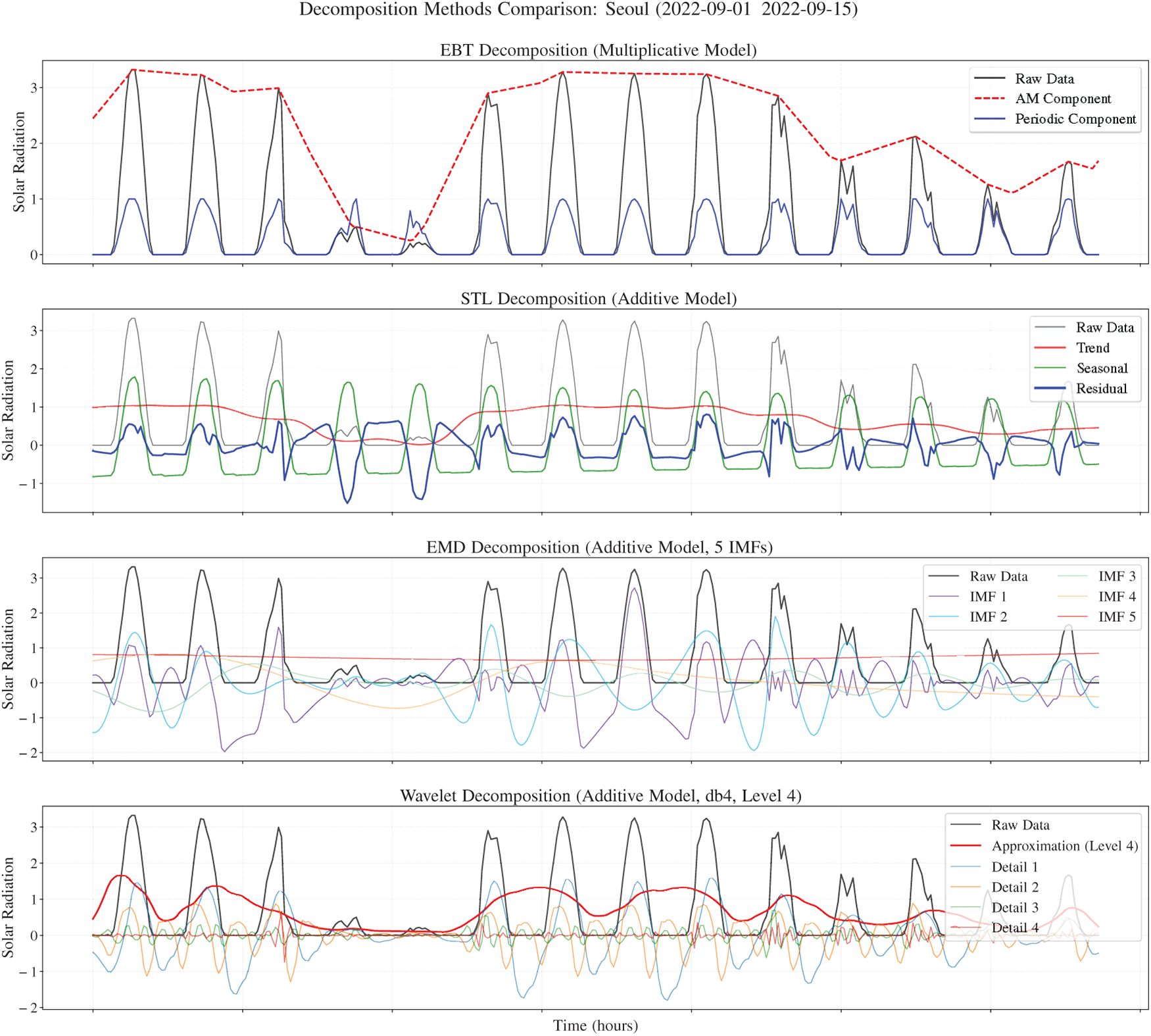
Figure A1: Decomposition comparisons on the raw-scale irradiance series for Seoul (2022-09-01 to 2022-09-15). Top: EBT multiplicative decomposition into amplitude modulation and periodic components. Middle rows: STL and EMD additive decompositions. Bottom: Wavelet (db4, level 4) additive decomposition

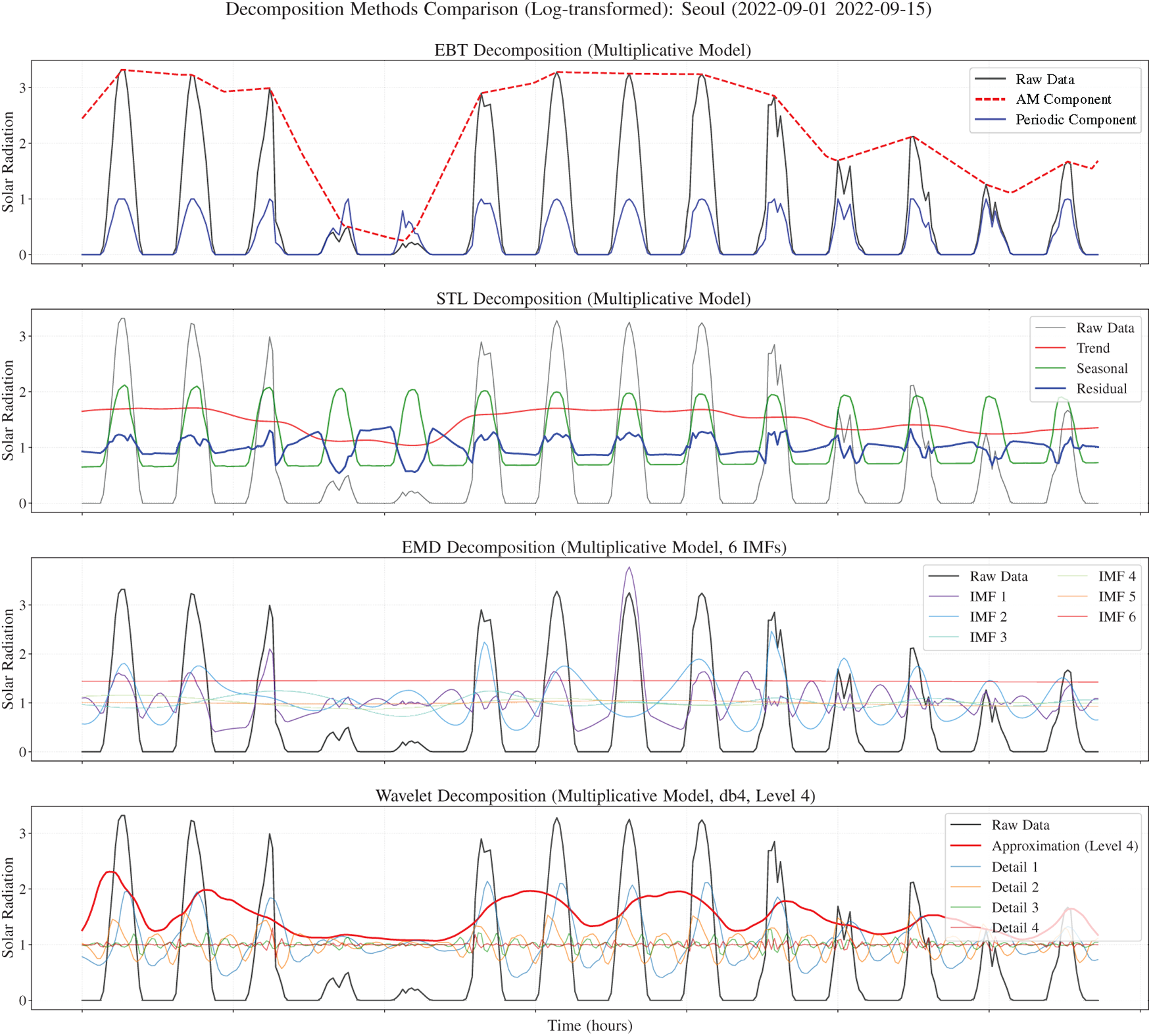
Figure A2: Decomposition comparisons on the log-transformed irradiance series for Seoul (2022-09-01 to 2022-09-15). Top: EBT multiplicative decomposition. Middle rows: STL and EMD multiplicative decompositions. Bottom: Wavelet (db4, level 4) multiplicative decomposition

In Fig. A1, EBT produces two clean, interpretable pieces: an envelope that follows weather-driven peaks (clouds, storms, typhoon days) and a periodic pattern that captures the daily cycle. Multiplying them already recreates the raw series with negligible error. STL splits into trend, seasonal, and residual, but the residual still carries daily peaks; on clear days it even drops below zero to compensate—a problematic behavior for strictly non-negative solar irradiance. EMD explodes the signal into many IMFs (typically 8–12): some look like short-wave noise, others partly resemble the daily rhythm, leaving no clear “this is the seasonal part” boundary. The lack of a single component representing the daily cycle limits physical interpretability. Wavelet shows a similar problem—periodic energy is scattered across detail levels (D1–D4) and the approximation (A4) blurs trend and seasonality—so a faithful, interpretable recomposition into envelope and cycle is not straightforward. In short, among the additive experiments, only EBT isolates the dominant daily cycle without leaking it into the residual.

For the multiplicative view, we first take logs (as in STL’s multiplicative option) so that all methods can operate additively and the components, once exponentiated, multiply back to the original. In Fig. A2, EBT again gives a crisp envelope plus periodic factor that recombine neatly with near-perfect reconstruction. STL still leaves daily remnants in the residual and the exponential of negative log-residuals produces values less than 1, implying non-physical compensation on clear days. EMD and Wavelet continue to spread periodic content across IMFs or detail bands, making it hard to point to a single periodic factor. While the log-transform imposes a multiplicative interpretation, it does not resolve the core issue: neither method provides a clear, two-component factorization into amplitude envelope and periodic cycle.

The comparative analysis highlights several advantages of EBT for solar irradiance forecasting. First, EBT’s factorization (yt=ytU×ytP) directly corresponds to the physical mechanism—a deterministic astronomical cycle modulated by stochastic weather—whereas STL, EMD, and Wavelet produce multi-component decompositions (trend + seasonal + residual, multiple IMFs, or approximation + multiple details) that do not map cleanly onto this structure. Second, EBT fully isolates the daily cycle in ytP, leaving ytU as a purely aperiodic amplitude signal. This clean separation is crucial for the proposed STGNN framework, which models each component with architectures tailored to its characteristics. STL leaves periodic remnants in the residual, while EMD and Wavelet spread periodic energy across multiple terms, complicating component-specific modeling. Third, EBT achieves perfect reconstruction with just two components, while STL requires three with remaining unexplained variance, and EMD/Wavelet require 8–12 terms for comparable accuracy. Fourth, solar irradiance is strictly non-negative with inherently multiplicative amplitude variations (e.g., cloud cover reduces irradiance by a factor, not a fixed amount), and EBT’s multiplicative framework naturally respects this structure.

We emphasize that EBT is not universally superior—STL excels for additive seasonal series (e.g., temperature anomalies), EMD for non-stationary oscillations (e.g., seismic data), and Wavelets for multiscale analysis (e.g., turbulence). However, for solar irradiance and similar multiplicative phenomena (e.g., wind power, tidal energy), EBT’s envelope-times-cycle decomposition provides a more natural and interpretable framework. By aligning the decomposition with the physical generation process, we enable more targeted modeling strategies, improve forecast accuracy (as demonstrated in Section 4), and facilitate better understanding of model behavior under extreme conditions (as shown in the Typhoon Hinnamnor case study).

Appendix B

This appendix presents additional experimental results for conventional non-spatial architectures—Temporal Convolutional Network (TCN), Long Short-Term Memory (LSTM), and Convolutional Neural Network-LSTM (CNN-LSTM) hybrid—to provide baseline comparisons with the STGNN models presented in the main text. We tested 36 configurations: 3 models × 3 lags (L∈{8,12,24}) × 4 capacity levels (filters/hidden units ∈{8,16,24,32}). Each configuration was trained for 2000 epochs with 10 independent runs, using the same 80/20 train/test split as the main experiments.

Table A1 shows the Classic baseline MSE results (mean ± std). TCN achieves the best performance among non-spatial models (MSE = 0.0601±0.0012 with lag 24, 32 filters), followed by LSTM (MSE = 0.0841±0.0023 with lag 8, 32 hidden units) and CNN-LSTM (MSE = 0.0975±0.0037 with lag 8, 32 filters). However, all three architectures substantially underperform compared to the STGNN models in Table 2, where GConvGRU and GConvLSTM achieve MSE ≈0.040 with only 20 epochs of training. This performance gap confirms that spatial correlation modeling through graph structures is crucial for multi-site solar radiation forecasting, validating our preference for STGNN architectures.

References

1. International Energy Agency. Renewables 2022: analysis and forecast to 2027. 2022 [cited 2025 Dec 2]. Available from: https://www.iea.org/reports/renewables-2022. [Google Scholar]

2. International Energy Agency. Net zero by 2050: a roadmap for the global energy sector. 2021 [cited 2025 Dec 2]. Available from: https://www.iea.org/reports/net-zero-by-2050. [Google Scholar]

3. Luthander R, Widén J, Nilsson D, Palm J. Photovoltaic self-consumption in buildings: a review. Appl Energy. 2015;142:80–94. doi:10.1016/j.apenergy.2014.12.028. [Google Scholar] [CrossRef]

4. Nwaigwe K, Mutabilwa P, Dintwa E. An overview of solar power (PV systems) integration into electricity grids. Mat Sci Energy Technol. 2019;2(3):629–33. doi:10.1016/j.mset.2019.07.002. [Google Scholar] [CrossRef]

5. Huld T, Müller R, Gambardella A. A new solar radiation database for estimating PV performance in Europe and Africa. Solar Energy. 2012;86(6):1803–15. doi:10.1016/j.solener.2012.03.006. [Google Scholar] [CrossRef]

6. Sengupta M, Xie Y, Lopez A, Habte A, Maclaurin G, Shelby J. The national solar radiation data base (NSRDB). Renew Sustain Energy Rev. 2018;89:51–60. doi:10.1016/j.rser.2018.03.003. [Google Scholar] [CrossRef]

7. Antonanzas J, Osorio N, Escobar R, Urraca R, Martinez-de Pison FJ, Antonanzas-Torres F. Review of photovoltaic power forecasting. Solar Energy. 2016;136:78–111. doi:10.1016/j.solener.2016.06.069. [Google Scholar] [CrossRef]

8. Yang D, Kleissl J, Gueymard CA, Pedro HT, Coimbra CF. History and trends in solar irradiance and PV power forecasting: a preliminary assessment and review using text mining. Solar Energy. 2018;168:60–101. doi:10.1016/j.solener.2017.11.023. [Google Scholar] [CrossRef]

9. Wan C, Zhao J, Song Y, Xu Z, Lin J, Hu Z. Photovoltaic and solar power forecasting for smart grid energy management. CSEE J Pow Energy Syst. 2015;1(4):38–46. doi:10.17775/cseejpes.2015.00046. [Google Scholar] [CrossRef]

10. Liu ZF, Li LL, Tseng ML, Lim MK. Prediction short-term photovoltaic power using improved chicken swarm optimizer-extreme learning machine model. J Clean Prod. 2020;248:119272. doi:10.1016/j.jclepro.2019.119272. [Google Scholar] [CrossRef]

11. Chu Y, Li M, Coimbra CF, Feng D, Wang H. Intra-hour irradiance forecasting techniques for solar power integration: a review. iScience. 2021;24(10):103136. doi:10.1016/j.isci.2021.103136. [Google Scholar] [PubMed] [CrossRef]

12. Hochreiter S, Schmidhuber J. Long short-term memory. Neural Comput. 1997;9(8):1735–80. doi:10.1162/neco.1997.9.8.1735. [Google Scholar] [PubMed] [CrossRef]

13. Agga A, Abbou A, Labbadi M, El Houm Y. Short-term self consumption PV plant power production forecasts based on hybrid CNN-LSTM, ConvLSTM models. Renew Energy. 2021;177:101–12. doi:10.1016/j.renene.2021.05.095. [Google Scholar] [CrossRef]

14. Bai S, Kolter JZ, Koltun V. An empirical evaluation of generic convolutional and recurrent networks for sequence modeling. arXiv:1803.01271. 2018. [Google Scholar]

15. Lim B, Arık SÖ., Loeff N, Pfister T. Temporal fusion transformers for interpretable multi-horizon time series forecasting. Int J Forecast. 2021;37(4):1748–64. doi:10.1016/j.ijforecast.2021.03.012. [Google Scholar] [CrossRef]

16. Li Y, Yu R, Shahabi C, Liu Y. Diffusion convolutional recurrent neural network: data-driven traffic forecasting. arXiv:1707.01926. 2017. [Google Scholar]

17. Yu B, Yin H, Zhu Z. Spatio-temporal graph convolutional networks: a deep learning framework for traffic forecasting. arXiv:1709.04875. 2017. [Google Scholar]

18. Wu Z, Pan S, Long G, Jiang J, Zhang C. Graph wavenet for deep spatial-temporal graph modeling. arXiv:1906.00121. 2019. [Google Scholar]

19. Wu Z, Pan S, Long G, Jiang J, Chang X, Zhang C. Connecting the dots: multivariate time series forecasting with graph neural networks. In: Proceedings of the 26th ACM SIGKDD International Conference on Knowledge Discovery & Data Mining; New York, NY, USA: ACM; 2020. p. 753–63. [Google Scholar]

20. Cui Z, Ke R, Pu Z, Ma X, Wang Y. Learning traffic as a graph: a gated graph wavelet recurrent neural network for network-scale traffic prediction. Transport Res Part C Emerg Technol. 2020;115:102620. doi:10.1016/j.trc.2020.102620. [Google Scholar] [CrossRef]

21. Choi G, Oh HS. Elastic-band transform for visualization and detection. Pattern Recogn Lett. 2023;166:119–25. doi:10.1016/j.patrec.2023.01.010. [Google Scholar] [CrossRef]

22. Choi G, Oh HS. Decomposition via elastic-band transform. Pattern Recogn Lett. 2024;182:76–82. doi:10.1016/j.patrec.2024.04.013. [Google Scholar] [CrossRef]

23. Bai L, Yao L, Li C, Wang X, Wang C. Adaptive graph convolutional recurrent network for traffic forecasting. Adv Neural Inform Process Syst. 2020;33:17804–15. [Google Scholar]

24. Li F, Feng J, Yan H, Jin G, Yang F, Sun F, et al. Dynamic graph convolutional recurrent network for traffic prediction: benchmark and solution. ACM Trans Know Disc Data. 2023;17(1):1–21. doi:10.1145/3532611. [Google Scholar] [CrossRef]

25. Shao Z, Zhang Z, Wei W, Wang F, Xu Y, Cao X, et al. Decoupled dynamic spatial-temporal graph neural network for traffic forecasting. arXiv:2206.09112. 2022. [Google Scholar]

26. Gu J, Jia Z, Cai T, Song X, Mahmood A. Dynamic correlation adjacency-matrix-based graph neural networks for traffic flow prediction. Sensors. 2023;23(6):2897. doi:10.3390/s23062897. [Google Scholar] [PubMed] [CrossRef]

27. Choi G, Oh HS. Exploring multiscale methods: reviews and insights. J Korean Statist Soc. 2025;54:1323–60. [Google Scholar]

28. Huang NE, Shen Z, Long SR, Wu MC, Shih HH, Zheng Q, et al. The empirical mode decomposition and the Hilbert spectrum for nonlinear and non-stationary time series analysis. Proc Royal Soc London Ser A Math Phys Eng Sci. 1998;454(1971):903–95. doi:10.1098/rspa.1998.0193. [Google Scholar] [PubMed] [CrossRef]

29. Cleveland RB, Cleveland WS, McRae JE, Terpenning I. STL: a seasonal-trend decomposition procedure based on loess. J Off Stat. 1990;6(1):3–73. [Google Scholar]

30. Mallat SG. A theory for multiresolution signal decomposition: the wavelet representation. IEEE Trans Pattern Analy Mach Intell. 2002;11(7):674–93. doi:10.1109/34.192463. [Google Scholar] [CrossRef]

31. Rozemberczki B, Scherer P, He Y, Panagopoulos G, Riedel A, Astefanoaei M, et al. Pytorch geometric temporal: spatiotemporal signal processing with neural machine learning models. In: Proceedings of the 30th ACM International Conference on Information & Knowledge Management; New York, NY, USA: ACM; 2021. p. 4564–73. [Google Scholar]

32. Seo Y, Defferrard M, Vandergheynst P, Bresson X. Structured sequence modeling with graph convolutional recurrent networks. In: International Conference on Neural Information Processing; Cham, Switzerland: Springer; 2018. p. 362–73. [Google Scholar]

33. Zhao L, Song Y, Zhang C, Liu Y, Wang P, Lin T, et al. T-GCN: a temporal graph convolutional network for traffic prediction. IEEE Trans Intell Transport Syst. 2019;21(9):3848–58. doi:10.1109/tits.2019.2935152. [Google Scholar] [CrossRef]

34. Diebold FX, Mariano RS. Comparing predictive accuracy. J Bus Econ Stat. 1995;13(3):253–63. [Google Scholar]

35. National Institute of Informatics. Digital Typhoon: Typhoon 202211 (HINNAMNOR); 2022 [cited 2025 Nov 21]. Available from: https://agora.ex.nii.ac.jp/digital-typhoon/summary/wnp/s/202211.html.en. [Google Scholar]