Bias Calibration under Constrained Communication Using Modified Kalman Filter: Algorithm Design and Application to Gyroscope Parameter Error Calibration

1  Introduction

In traditional digital control systems, data is typically transmitted under limited communication resources. A typical solution to conduct data transmission under limited communication resources is to employ the event-triggered mechanism, which operates on the principle that whenever a sampling period elapses. The transmission system exchanges data regardless of whether the current data are useful. This event-triggered mechanism approach is relatively simple to implement in engineering cases and offers advantages such as ease of system analysis and conciseness of controller design. As a result, research on event-triggered techniques has become increasingly important in the case of limited communication resources [1,2].

To effectively reduce the consumption of communication resources in control systems, a novel control mechanism, event-triggered control has been proposed [3,4]. A brief comparison between event-triggered control and time-triggered control has been given in [5] to highlight the advantages of the event-triggered mechanism. Closely following, an event-triggered scheduling algorithm has been designed in [6] for a class of nonlinear networked control systems. Subsequently, a new event-triggered scheme termed the dynamic event-triggered scheme has been devised in [7] which differs from previous schemes by incorporating an internal variable to characterize the triggering instants. Currently, a growing number of researchers are applying event-triggered control strategies to various control and estimation problems, such as tracking [8], estimation [9,10], and robust control [11].

The optimal state estimation means to find the accurate state of the system based on the collected sensor information. A commonly used state estimation approach is the error correction algorithm, which most favor linear systems with known parameters and noises following known first and second statistics [12–14]. References [15,16] proposed a Tobit error correction algorithm for state estimation in right-sensored models. Reference [17] proposed a two-stage error correction for noise estimation. Reference [18] proposed a reduced-order error correction to constrain data for state-constrained linear systems. Reference [19] designed a new cost function in error correction to tackle linear noisy questions. Reference [20] proposed an online exploratory maximum likelihood estimation approach to adaptive Kalman filtering. Reference [21] proposed a Measurement and Process Noise Covariance Estimation Using Kalman Smoothing. When it comes to the case of measurement bias, the error correction would fail to come up with the optimal estimation and even produce bad state estimates. This is just the case under the event-triggered scheme. More specifically, as the event-triggered scheme only transmits a sensor measurement when it falls inside/outside a predefined threshold, measurement bias is unavoidably incurred between the transmitted and untransmitted measurements. This undoubtedly results in parameter variations of the system and measurement parameters, thereby giving rise to deteriorated performance of the error correction. As such, there is an urgent need to develop a bias calibration framework to ensure the optimality of the error correction under the limited-communication-induced sensor bias.

Motivated by the above observation, this paper proposes a novel bias calibration algorithm under communication constraints to achieve accurate system states of the interested system. An output-based event-triggered scheme is first employed to alleviate transmission burden, and accounting for the limited-communication-induced measurement bias, a novel bias calibration algorithm based on the Kalman filtering line is developed to restrain the effect of the measurement bias on the system estimation, thereby achieving accurate system state estimates. Subsequently, the FPGA implementation of the proposed algorithm is also realized with the hope of providing fast bias calibration in practical scenarios. A numerical example and a practical example (for the gyroscope’s angular velocity bias calibration) on MATLAB are both provided to demonstrate the feasibility and effectiveness of the proposed algorithm.

The main contributions of this paper are as follows. (1) A novel bias calibration algorithm is proposed based on the error correction framework that effectively constrain the bias effect on the state estimation performance under the event-triggered mechanism. (2) The FPGA implementation of the proposed algorithm is used to provide fast and real-time bias calibration and state estimation in practical scenarios. (3) A gyroscope example is employed to verify the feasibility of the proposed algorithm in tackling real-world application problems.

2  Basic Principle

2.1 Kalman Filter

The error correction is a primary data regression estimation tool in the field of data processing, commonly used for estimating the state of dynamic systems with measurement noise. This algorithm is a minimum mean square error (MMSE) estimation algorithm. When the system’s state equation and measurement equation are known, and the noise is assumed to follow a certain distribution (such as a Gaussian distribution, T-distribution, etc.), the error correction provides the statistically optimal estimate for the measured data. The classical error correction is suitable for linear Gaussian systems and can only reduce the impact of noise with zero mean on the system. If the noise expectation is zero, then regardless of the noise variance, as long as the error correction algorithm iterates sufficiently many times, it can eventually provide a good estimate of the system state. Conversely, if the noise expectation is non-zero, no matter how many iterations are performed, the estimate obtained by the error correction algorithm will still deviate from the true value. The classical error correction algorithm can be described by the following set of recursive mathematical formulas:

x^k|k−1=Ax^k−1|k−1,(1)

Pk|k−1=APk−1|k−1AT+Q,(2)

x^k|k=x^k|k−1+Kk(zk−Hx^k|k−1),(3)

Kk=Pk|k−1HT(HPk|k−1HT+R)−1,(4)

Pk|k=(I−KkH)Pk|k−1(5)

where zk is the observation at the current time step, x^k|k is the posterior estimated state vector at time k, x^k|k−1 is the prior estimate from the error correction at time k, A is the state transition matrix of the observation model, transforming the state from time k – 1 to time k, C is the measurement matrix of the observation model, Kk is the Kalman gain at time k, Q is the process noise covariance, Pk|k is the posterior error covariance matrix at time k, Pk|k−1 is the prior error covariance matrix from the Kalman filter, and R is the measurement noise covariance.

2.2 Event-Triggered Mechanism

The event-triggered mechanism, also known as the event-driven mechanism, is a data transmission mechanism that employs passive sampling updates. Its core idea is that the control system transmits sensor signals or updates control signals only when certain conditions are met. In other words, when using event-triggered control for data transmission, data is transmitted from the sensor to the estimator or information fusion center only when a specific event occurs.

Based on different establishment criteria, common event-triggered schemes can be classified into the following three types: i.e., state error-based, input error-based, and measurement output-based event-triggered schemes. From the description of the several event-triggered mechanisms above, it can be seen that the establishment conditions of both the state error-based and input error-based event-triggered mechanisms are related to the system state. This allows the estimator to have more sufficient and complete information for subsequent anomaly detection. However, both types of event-triggered mechanisms require the estimator to compute the estimated value for each state. Therefore, when the amount of information to be transmitted is large, the data volume can become very large, significantly increasing the system’s communication and computational costs, which will burden the system.

In this paper, the output-based event-triggered mechanism is selected for data transmission, which can achieve the goal of saving communication resources without imposing excessive computational costs during system implementation.

3  Method

3.1 Event-Triggered Mechanism Design

In practical systems, communication networks often send some “unnecessary” data signals, wasting network bandwidth resources. Therefore, to save communication network resources, sensor nodes adopt an event-triggered mechanism to decide whether to send measurement data. Comprehensively considering computational complexity and the accuracy of the trigger mechanism, this thesis chooses to establish an event-triggered mechanism based on the system’s observed values. This paper employs a dead-zone-like event-triggered mechanism, setting a specific interval. It is assumed that the sensor sends a measurement value only when it falls outside this predetermined interval (i.e., the measurement value is greater than the upper limit of the interval or less than the lower limit).

Denoting the new measurement data obtained by the detection unit as yk, the established event-triggered mechanism can be expressed by Eq. (6):

yk(l)={zk,zk≥ThTm,Tl<zk<Thzk,zk≤Tl(6)

where Th and Tl represent the trigger thresholds of the event-triggered mechanism. Assume Tm=(Th+Tl)/2. The specific event-triggered conditions are as follows:

(1) When the trigger condition (zk−Th)×(zk−Tl)≥0 is satisfied, the current observation value is transmitted to the detection unit, i.e., yk=zk.

(2) When the trigger condition (zk−Th)×(zk−Tl)≥0 is not satisfied, the current observation value is not transmitted to the detection unit. The untransmitted measurement value is replaced by the corresponding element in Tm at the detection unit, i.e., yk=Tm. Based on the statistical characteristics of a system with normally distributed error, the expectation and variance of the transmitted value after passing through the event-triggered mechanism can be calculated, as shown in Eqs. (7) and (8).

E(yk|xk,σ)=(1−ϕ(Th−Cxkσ))(Cxk+σλ(Th−Cxkσ))+(ϕ(Th−Cxkσ)−ϕ(Tl−Cxkσ))Tm+ϕ(Cxk−Tlσ)(Cxk−σλ(Cxk−Tlσ))(7)

var(yk|xk,σ)=(1−ϕ(Th−Cxkσ))σ2(1−∂(Th−Cxk))+ϕ(Tl−Cxkσ)σ2(1−∂(Cxk−Tl))(8)

λ(α)=φ(α)1−ϕ(α)(9)

∂(α)=λ(α)(λ(α)−α)(10)

where ϕ(α) represents the cumulative distribution function (CDF) of the standard normal distribution, and φ(α) represents the probability density function (PDF) of the standard normal distribution.

When a system is observed by multiple sensors, different trigger threshold intervals can be set for each sensor. Similarly, only observed values outside their respective threshold intervals are sent to the data detection center. Different threshold intervals lead to different trigger conditions for the system’s observed values, resulting in variations in the data transmitted through the event-triggered mechanism. Consequently, the performance of the event-triggered module and the data detection module will also differ. Generally, a larger threshold interval results in a lower trigger rate, saving more communication resources. However, simultaneously, more information remains untransmitted, meaning the filter has less data available for state estimation, which can lead to a reduction in the estimation accuracy of the filter estimator. The selection of the trigger threshold interval is jointly determined by the estimator’s estimation accuracy and the communication efficiency of the transmission unit. By changing the trigger threshold of the event-triggered mechanism, the transmission efficiency of signals can be altered, which also affects the subsequent data processing results to some extent.

3.2 Bias Calibration under the Modified Kalman Filtering

Taking a general linear system as the research object, in the absence of anomalous data, the object observed by the sensor can be described by the following two equations:

xk=Axk−1+wk−1(11)

zk=Cxk+vk(12)

here, Eq. (11) is the system’s state transition equation, where xk∈Rn×1 represents the system’s state vector at time k. Eq. (12) is the system’s measurement equation, where zk∈Rm×1 represents the sensor’s measurement output vector at time k. A is the system’s state transition matrix, and C is the system’s observation matrix; both are constant coefficient matrices with appropriate dimensions. It is assumed that the state error wk is white noise with zero mean and covariance Q∈Rn×n, and the measurement error vk is white noise with zero mean and covariance R∈Rm×m, with standard deviation σ. They are uncorrelated with each other, and for i≠j, wi is uncorrelated with wj, and vi is uncorrelated with vj, satisfying the following conditions:

E[wiwjT]={Q,i=j0,i≠j(13)

E[vivjT]={R,i=j0,i≠j(14)

The standard Kalman filter algorithm is designed for the linear Gaussian system described by Eqs. (11) and (12). However, when an event-triggered mechanism is introduced into the model, the measurement values transmitted to the data detection unit exhibit a “dead zone” like output characteristic. The data received by the detection unit no longer satisfies the assumptions of the standard Kalman filter. Therefore, the formulas of the standard Kalman filter algorithm need modification; specifically, the cross-covariance, output covariance, and state covariance cannot be calculated using the standard KF formulas. The state prediction equation and state covariance prediction equation of the Kalman filter are calculated based on the system model parameters and thus do not require correction. The derivation principle for the relevant Kalman filter parameters is the minimization of the system’s state error covariance. Based on this, the measurement update part of the Kalman filter algorithm is modified. For the system described by Eqs. (6), (11) and (12), the modified Event-Triggered Kalman Filter (ETKF) must be used for estimating the system state. The modified Kalman filter equations are shown in Eqs. (15) to (21) [22]:

x^k|k−1=Ax^k−1|k−1(15)

Pk|k−1=APk−1|k−1AT+Q(16)

x^k|k=x^k|k−1+Kk(yk−E(yk|x^k|k−1))(17)

Pk|k=(Im×m−(E(ξk)+E(ζk))KkC)Pk|k−1(18)

Kk=Rxyk(Ryyk)−1(19)

Ryyk=(E(ξk)+E(ζk))CPk|k−1CT(E(ξk)+E(ζk))+E[(ξk+ζk)vkvkT(ξk+ζk)](20)

Rxyk=Pk|k−1CT(E(ξk)+E(ζk))(21)

where x^k|k−1 and x^k|k represent the prior and posterior estimated states at time k, respectively; Pk|k−1 and Pk|k represent the prior and posterior state error covariance matrices at time k, respectively; Rxyk is the cross-covariance; Ryyk is the system output covariance; ξk and ζk are introduced Bernoulli random variables. Reference [22] has discussed the validity of using x^k|k−1 in place of x^k|k. When the sensor’s observation value is transmitted, the Bernoulli random variable takes the value 1.

When it is not transmitted, it takes the value 0. These Bernoulli random variables are introduced to better model the received data yk at the detection unit. The means of these two Bernoulli random variables can be calculated using the following formulas:

E[diag(ξk(l))]l×l≈diag(ϕ(Tl−Cx^k|k−1(l)σ(l)))l×l(22)

E[diag(ζk(l))]l×l≈diag(1−ϕ(Th−Cx^k|k−1(l)σ(l)))l×l(23)

E[(ξk+ζk)vkvkT(ξk+ζk)]=diag(var(yk(l)−Cx^k|k−1(l)|σ(l)))m×m(24)

where l=1,…,m denotes the l-th element. When no system bias exists, the system state value based on the event-triggered mechanism can be estimated according to the above algorithm using the measurement values and system model parameters. However, in many practical applications, sensor observation systems always contain system bias. If the system bias is not detected, it will be impossible to know whether the observed data is normal or not, and also impossible to know whether the estimated system state is the actual state of the system. From Eqs. (22) to (24), it can be seen that the variables ξk and ζk are related to the transmission thresholds Tl and Th, the state x^k, and the state noise wk. In Eqs. (23) and (24), the estimated value x^k|k−1 is used to replace the state x^k. This approximation is based on the unbiased estimation property of the Kalman filter. Therefore, when the system modeling is reasonable—that is, when the selected A, Q, and R matrices are appropriate—the error introduced by this approximation becomes acceptable, and the influence of measurement noise vk on the estimated value x^k|k−1 will be filtered out. Thus, under such conditions, the variables ξk and ζk are independent of the measurement noise vk. Different from only one threshold of the Tobit Kalman Filter, the proposed algorithm has two thresholds to make the event-triggered work as shown in Table 1. Therefore, the expectation and variance of the transmitted value are different from Tobit Kalman Filter. Besides, the Tobit Kalman filter is mainly aimed at the truncation errors generated by sensors, but the proposed algorithm targets the errors that occur under communication constraints.

4  Experiment

4.1 Event-Triggered Algorithm Simulation

The feasibility of the algorithm is verified through simulation experiments, using the general linear system described by Eqs. (11) and (12) as an example. To better observe the experimental results, the state transition matrix is taken as a rotation matrix:

A=[cos⁡(β)−sin⁡(β)sin⁡(β)cos⁡(β)]

The measurement matrix is C=[10]. The state error covariance is Q=diag(0.012,0.022), the measurement error covariance is R=2, and the standard deviation is σ=2. The initial system state is set to x0=[1,0]T, the initial state covariance is P=diag(1,1), the model parameter is chosen as β=0.016, the sampling period is set to 1 s, and the total sampling time is 2000 s.

When this linear system model is observed by multiple sensors, different trigger threshold intervals can be set. This experiment uses four pairs of event-triggered thresholds and compares their results: Threshold 1: Th=0.5, Tl=−0.5; Threshold 2: Th=1, Tl=−1; Threshold 3: Th=2, Tl=−2; Threshold 4: Th=2.5, Tl=−2.5. The simulation results for these four thresholds are shown in Fig. 1. From Fig. 1, it can be seen that regardless of the event- triggered threshold interval, the amplitude of the measured output is effectively acquired only outside the “dead zone”, i.e., only when the measurement value is less than Tl or greater than Th is it sent to the data detection unit. However, when the measurement value is greater than Tl and less than Th, the actual measurement output is not sent to the data detection unit, and the untransmitted measurement value is replaced by Tm. Simultaneously, when the event-triggered threshold interval changes, the amount of data transmitted by the system and the number of time points requiring data communication also change. MATLAB software was used to calculate the trigger rates and communication resource saving rates corresponding to the above four threshold intervals. The calculation results are shown in Table 2:

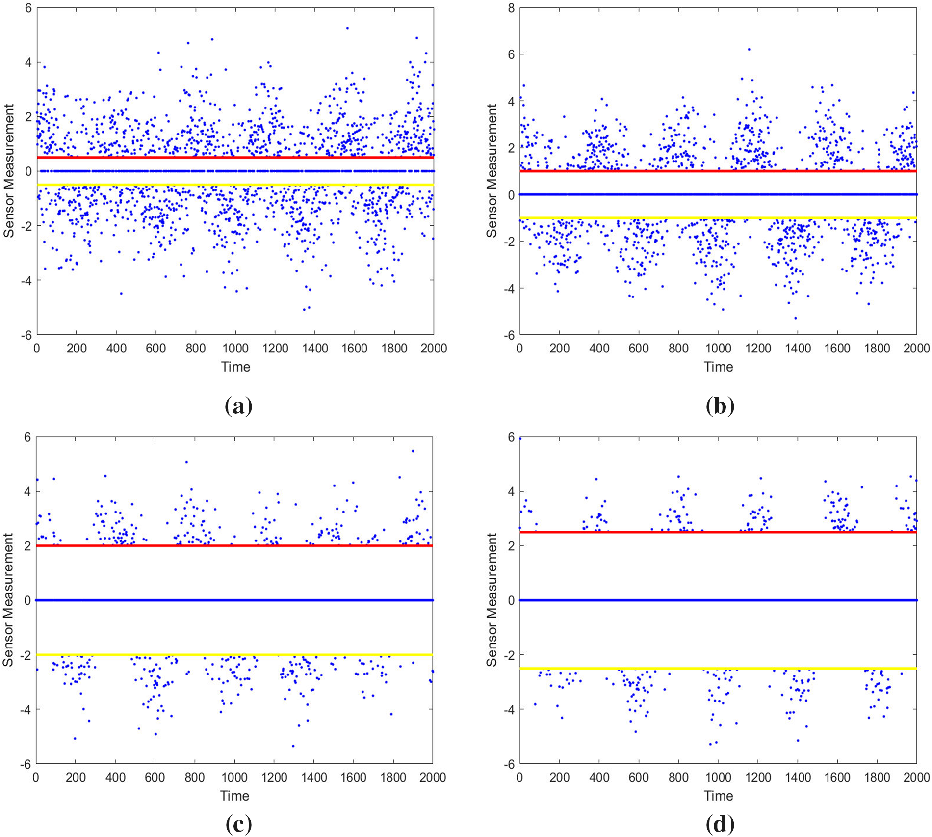
Figure 1: Event-triggered output. (a) Threshold 1; (b) Threshold 2; (c) Threshold 3; (d) Threshold 4

From the results in Table 2, it can be concluded that for the same observation system, different threshold settings lead to different trigger probabilities of the event-triggered mechanism and different amounts of saved communication resources. A larger threshold interval results in a lower trigger rate of the established event-triggered mechanism and saves more communication resources.

4.2 Numerical Example

First, assuming no system bias exists, the estimation of the system state by the event-based error correction algorithm is verified. The simulation object remains the general linear system described by Eqs. (11) and (12). The system model parameters are the same as those used in the previous section for the event-triggered algorithm. MATLAB is used to plot the state estimation results of the event-triggered error correction for the aforementioned four threshold intervals, as shown in Fig. 2. Meanwhile, an outline detection function is built in Fig. 3.

Figure 2: State estimation results without anomalous data. (a) Estimation result for X1; (b) Estimation result for X2

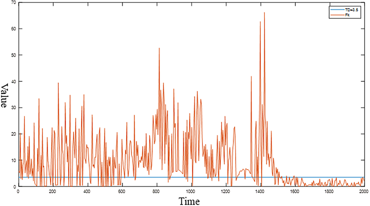
Figure 3: Outline detection function

The simulation results show that when system bias is absent, this event-triggered detection algorithm can estimate the state of the linear system well. Furthermore, different thresholds selected for the event-triggered mechanism lead to variations in the state estimation performance of the event-based error correction algorithm. The cumulative mean square error (AMSE) shown in Eq. (25) can be used to evaluate the estimation performance of the event-based error correction algorithm:

AMSE(k)=∑t=0k1N∑i=1N(xti−x^ti)2(25)

where xti is the true state at time t in the i-th experiment, and x^ti is the estimated state at time t in the i-th experiment. This experiment conducted 10 random trials, i.e., N=10. MATLAB is used to plot the cumulative mean square errors corresponding to the four threshold intervals, as shown in Fig. 4.

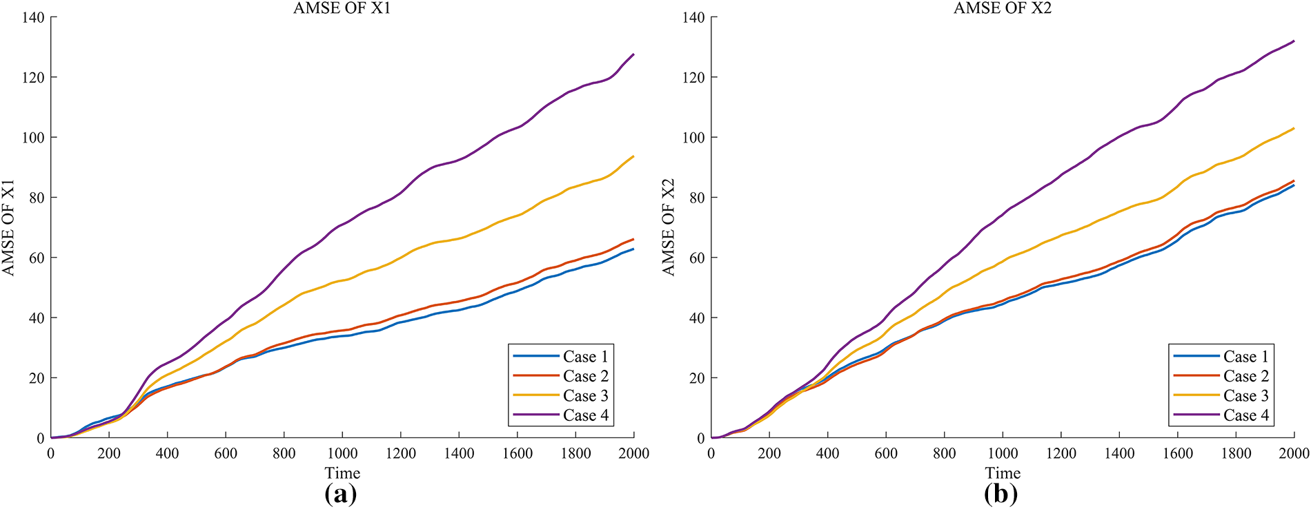
Figure 4: Cumulative mean square error of the event-based kalman filter. (a) AMSE(X1); (b) AMSE(X2)

From Fig. 4, it can be seen that the larger the threshold interval selected when establishing the event-triggered mechanism, the larger the cumulative mean square error between the estimated value obtained by the event-based error correction algorithm and the true value, indicating lower estimation performance of the estimator. Therefore, when selecting the threshold interval for a practical event-triggered mechanism, it is necessary to comprehensively consider the communication resource saving ratio and the estimation accuracy of the estimator. Meanwhile, the slopes of the cumulative mean square error graphs for all four selected thresholds gradually flatten out, indicating that the mean square errors for these four thresholds are bounded, meaning that the event-triggered mechanisms established using these four thresholds are stable.

The development platform used for the experiment is the Xilinx ZYNQ-7020 system, the EDA tool is Vivado 2019.1, and the hardware description language used is Verilog HDL. The system model and parameters are consistent with those used in the numerical simulation in the previous section.

First, the functionality of the event-triggered mechanism circuit is verified. The thresholds are selected as Th=2, Tl=−2. The simulation results are shown in Fig. 5:

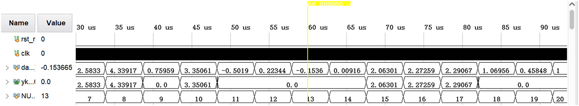
Figure 5: Simulation results of the event-triggered mechanism

In the figure, the first signal rstn is the reset signal, the second signal clk is the 50 MHz clock signal, the third signal datain is the sensor’s observed value, the fourth signal yk is the output of the event-triggered mechanism circuit, and the fifth signal NUM indicates the count of current input data. From the FPGA output results, it can be seen that when the sensor’s observed value is within the threshold interval (i.e., does not satisfy the event-triggered condition), the data is not transmitted but is replaced by 0; when the sensor’s observed value is outside the threshold interval (i.e., satisfies the event-triggered condition), the data is transmitted.

The output results of the FPGA-based event-triggered mechanism are imported into MATLAB, and the discrete point plot of the yk signal is drawn as shown in Fig. 6:

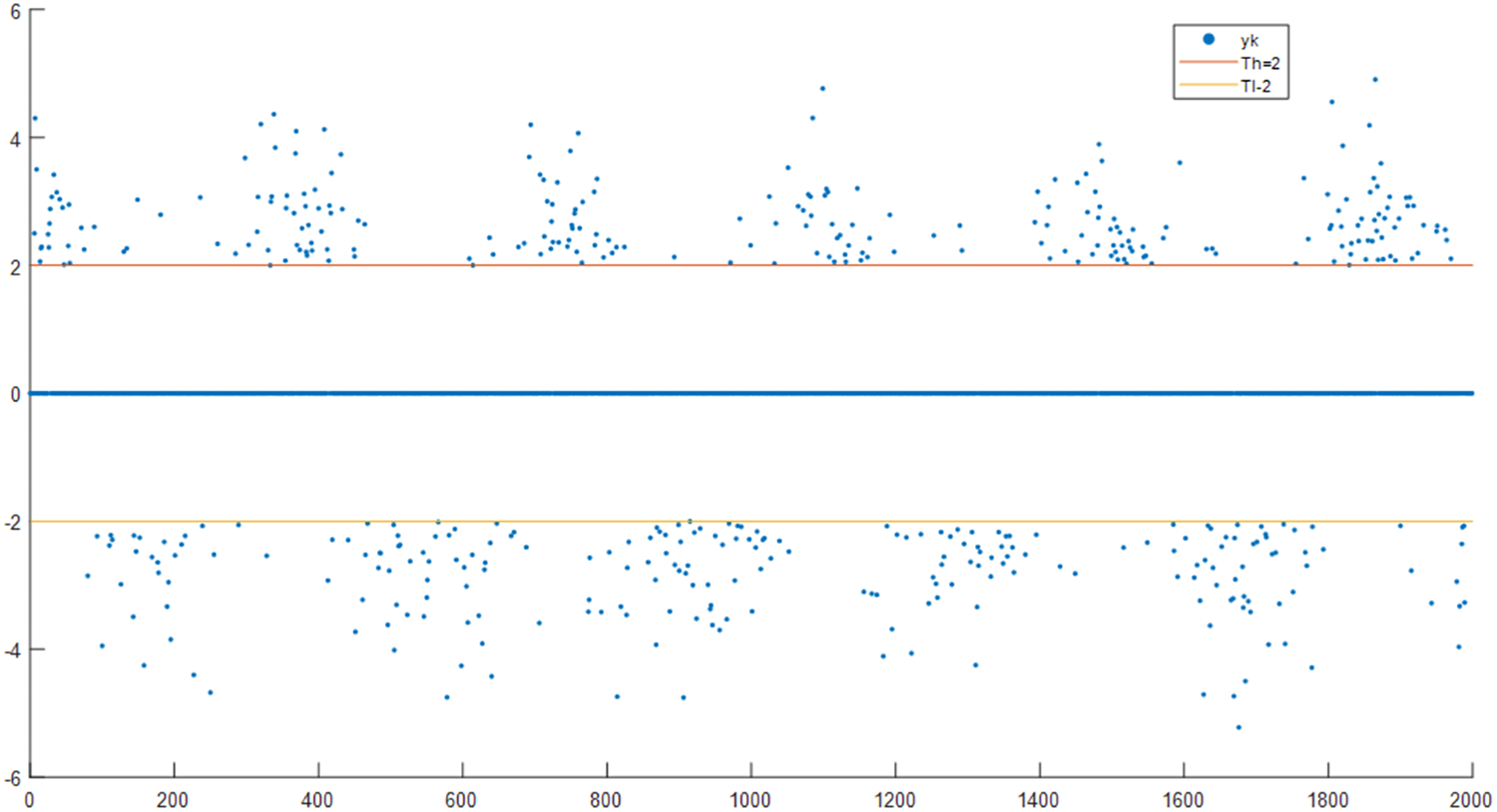
Figure 6: Output of the event-triggered circuit processed by MATLAB

From Fig. 6, it can be seen that for the FPGA-based event-triggered mechanism, only data outside the threshold interval is transmitted; that is, only data satisfying the event-triggered condition (less than Tl or greater than Th) is sent to the signal detection unit. Data within the threshold interval is replaced by the predetermined value Tm. This indicates that the FPGA circuit for the event-triggered mechanism has been successfully implemented.

The output results of the Verilog program for the event-based error correction and the signal waveform results are shown in Figs. 7 and 8, respectively:

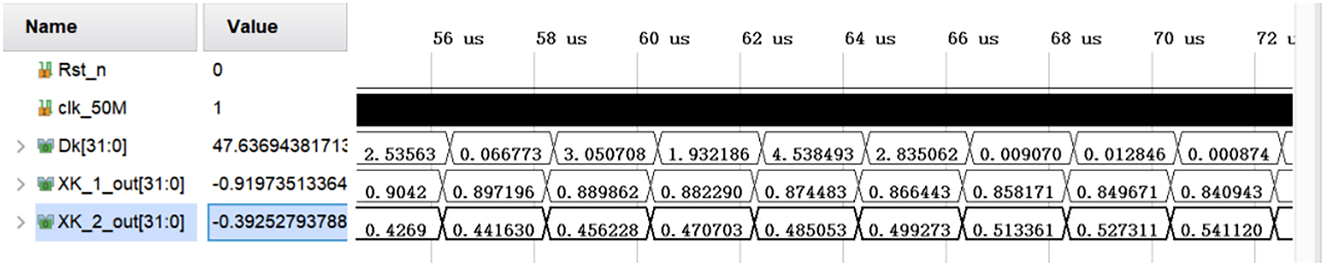
Figure 7: State estimation results

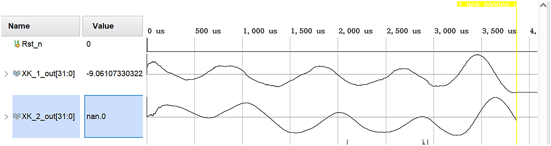
Figure 8: State estimation waveform diagram

This section details the processing of the gyroscope output data. The gyroscope was mounted on a rate table and rotated at a constant angular velocity to collect its output data, as illustrated in Fig. 9.

Figure 9: Experimental Setup (a) and The GUI of the data acquisition software (b)

With a properly configured rotation profile, the theoretical output of the gyroscope should be a trigonometric function. However, in practice, the output is susceptible to various interfering factors, resulting in a measured curve accompanied by error-induced glitches. By applying an event-triggered algorithm to the gyroscope data, the proposed bias calibration algorithm, we aim to correct the unexpected error of the data and recover the intended gyroscope output.

Analogous to the simulation experiment, the measurement transition matrix is taken as C=[10], while the state transition matrix is represented by a rotation matrix:

A=[cos⁡α−sin⁡αsin⁡αcos⁡α]

where α is the angular rotation rate of the gyroscope.

Based on the gyroscope output data, the system’s initial state is set to x0=[1.250], with a sampling period of 100 Hz for 2000 points. When this system model is observed by multiple sensors, the triggering thresholds are set to Th = 0.25, Tl = −0.25. The smoothed results of the data falling within these thresholds are shown in Fig. 10.

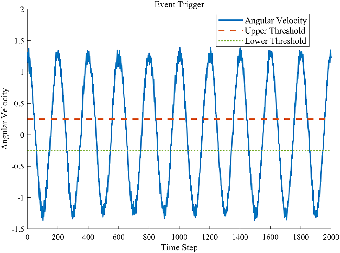
Figure 10: Image after event-triggered processing

Smoothing the data that falls within the threshold interval can suppress the impact of error on the overall dataset to some extent and partially save computational resources. The signals initially processed via the event-triggered mechanism are further filtered, and the results are compared with the gyroscope output measurements. The comparison is shown in Fig. 11a, with a locally enlarged view presented in Fig. 11b. The proposed algorithm can effectively smoothed the output.

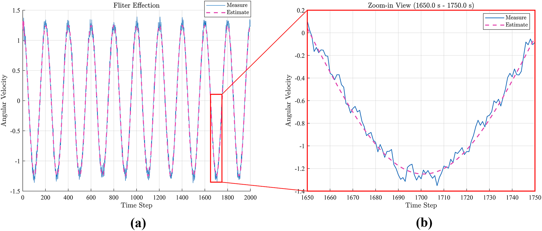
Figure 11: Output curve after error correction. (a) results of filter; (b) enlarged view of (a)

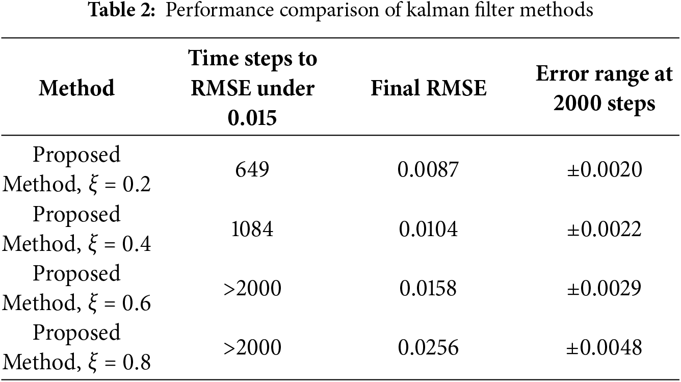
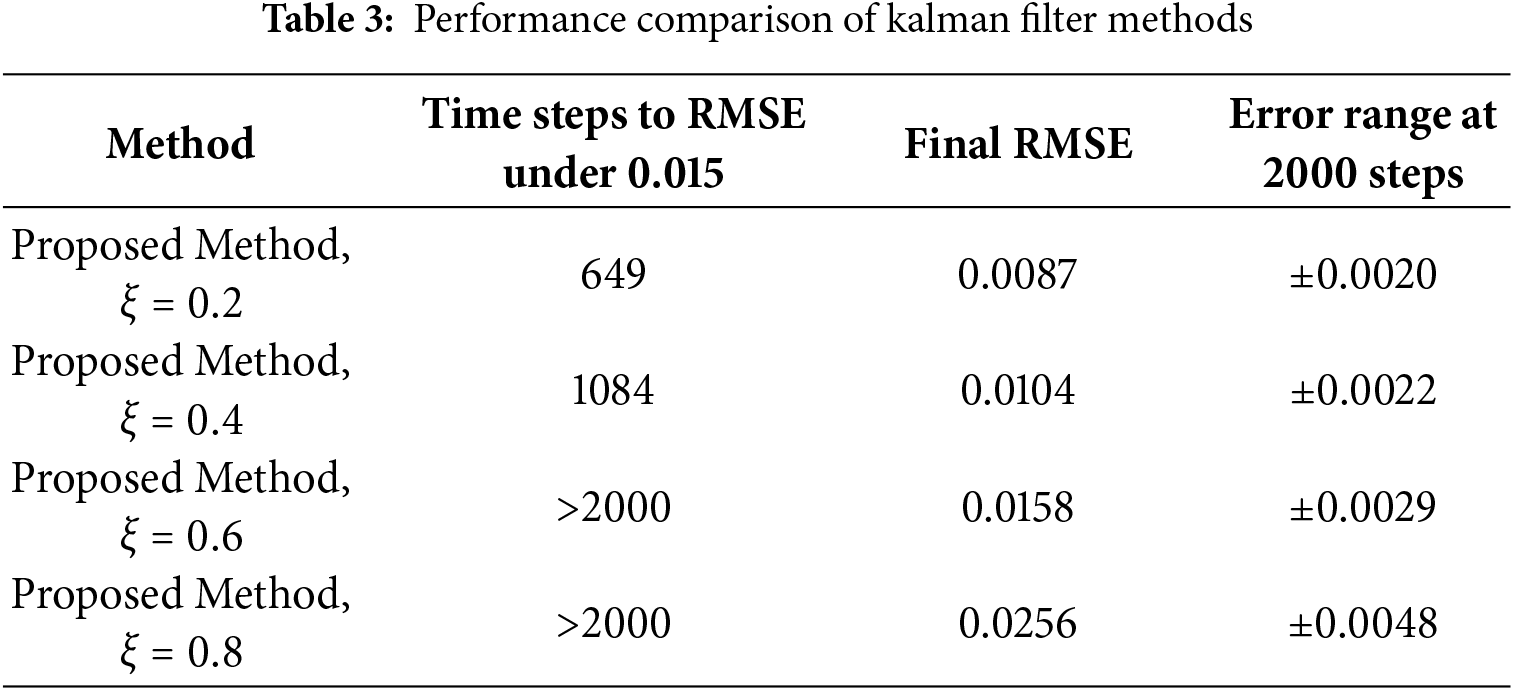
Besides, to determine the application scope and limitations of the proposed algorithm, this paper conducted experiments for threshold determination. As shown in Fig. 12 and Table 3, the experimental results indicate that when the threshold reaches 0.8, the Root Mean Square Error(RMSE) increases significantly. Therefore, the threshold range for this algorithm should be set between 0.05 and 0.8.

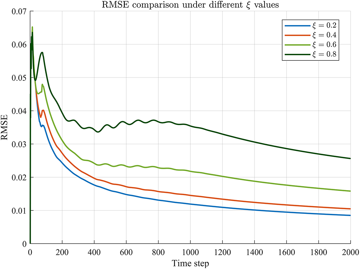
Figure 12: RMSE comparison of different thresholds

It can be observed that the curve processed by the error correction algorithm closely follows the theoretical curve. The overall waveform shows that the estimated values smoothly track the measurement trend, effectively suppressing high-frequency error. Fig. 13 illustrates the variation of the estimation error over time steps between this paper’s method (a) and the Kalman filter (b), with the error ultimately fluctuating within the range of ±0.003 in our method while Kalman filter is ±0.01, indicating that the algorithm maintains stable estimation accuracy throughout the entire time span.

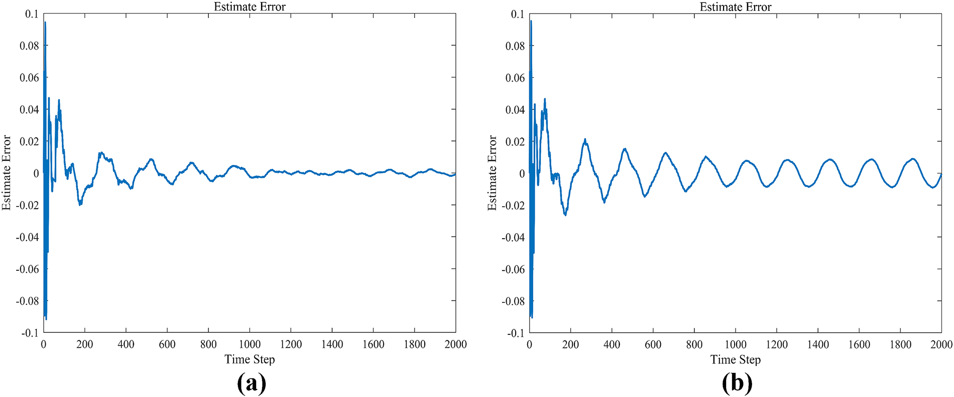
Figure 13: Comparison of our method and kalman filter

To further evaluate the error correction performance, RMSE is used as one of the evaluation metrics, calculated as follows:

RMSE=1n∑i=1n(xi−x^i)2

Fig. 14 presents the variation of RMSE over time of our method (a) and the Kalman filter (b). The RMSE gradually decreases from the initial stage and stabilizes below 0.0087, while the Kalman filter is 0.0109, and the proposed algorithm achieves an RMSE below 0.015 at the 649th data point, whereas the Kalman filter requires until the 889th point to reach the same level. This demonstrates the superior real-time performance of the proposed algorithm. This indicates that the algorithm exhibits fast convergence and robustness. The experimental results collectively demonstrate that the event-triggered error correction algorithm can effectively handle errors and abnormal fluctuations in gyroscope data. Through the event-triggered mechanism, the algorithm reduces unnecessary computations while maintaining estimation accuracy. Both error and RMSE curves confirm the stability of the algorithm, particularly during long-term operation, where the RMSE remains at a low level. These simulations validate the feasibility and effectiveness of the proposed algorithm for gyroscope data error correction, providing a reference for practical engineering applications.

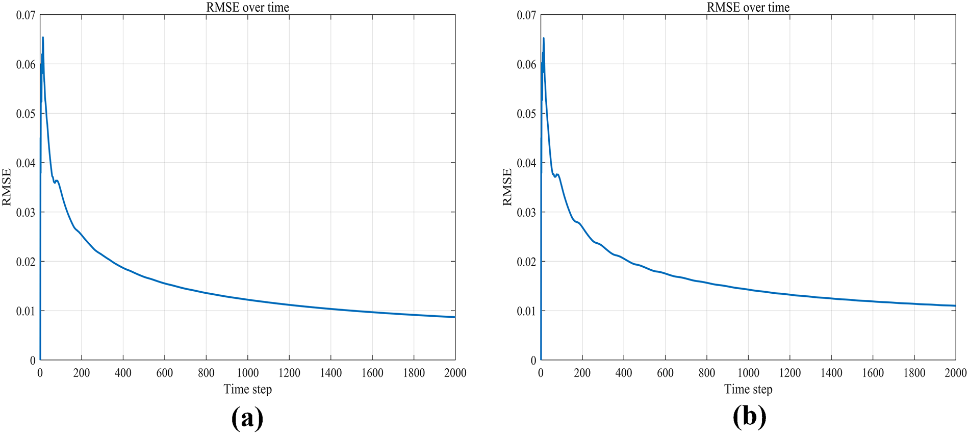
Figure 14: RMSE of our method and kalman filter. (a) RMSE of our method; (b) RMSE of Kalman Filter

5  Conclusion

This paper has proposed a novel bias calibration algorithm under communication constraints to achieve accurate system states of the interested system. An output-based event-triggered scheme has been first employed to alleviate transmission burden, and accounting for the limited-communication-induced measurement bias, a novel bias calibration algorithm based on the error correction line has been developed to restrain the effect of the measurement bias on the system estimation, thereby achieving accurate system state estimates. Subsequently, the FPGA implementation of the proposed algorithm has also been realized with the hope of providing fast bias calibration in practical scenarios. A numerical example and a practical example (for the gyroscope’s angular velocity bias calibration) have both been provided to demonstrate the feasibility and effectiveness of the proposed algorithm. However, the threshold for event triggering proposed in this paper is not adaptive, resulting in insufficient generalization performance of the algorithm. Meanwhile, the FPGA circuit designed in this paper requires 252 clock cycles to complete the processing of one set of data. Although it can effectively output the true state values of the data, it may not meet the high-speed requirements of some practical engineering applications. Therefore, future work should focus on developing an algorithm capable of adaptively adjusting the threshold to enhance the generalization performance of the proposed method. And further leverage the parallel computing principle of FPGAs to investigate how to improve the computational speed.

Acknowledgement: This research was supported by the National Natural Science Foundation of China and the Sichuan Science and Technology Program.

Funding Statement: This work received financial support from the National Natural Science Foundation of China (Grant Nos. U2330206, U2230206, and 62173068), and Sichuan Science and Technology Program (Grants Nos. 2024NSFSC1483, 2024ZYD0156, 2023NSFC1962, and DQ202412).

Author Contributions: Qi Li: Conceptualization, Methodology, Data curation, and Writing—original draft. Yifan Wang: Formal analysis, Supervision, Project administration, Review & editing (corresponding author). Yuxi Liu: Methodology, Software implementation and Result interpretation. Xingjing She: Investigation, Software implementation, Writing—original draft, and Result interpretation. Yixuan Wu: Software implementation, Writing—original draft, and Review & editing. All authors reviewed the results and approved the final version of the manuscript.

Availability of Data and Materials: The experimental data used in this study were acquired by a MEMS gyroscope via a self-developed platform at a sampling rate of 100 Hz. Due to commercial agreements, the dataset cannot be made publicly available. Parameter settings necessary to reproduce the results are provided, and further details are available from the corresponding author.

Ethics Approval: Not applicable.

Conflicts of Interest: The authors declare no conflicts of interest to report regarding the present study.

Nomenclature

References

1. Khashooei BA, Antunes DJ, Heemels WPMH. Output-based event-triggered control with performance guarantees. IEEE Transact Autom Cont. 2017;62(7):3646–52. doi:10.1109/tac.2017.2672201. [Google Scholar] [CrossRef]

2. Donkers MCF, Heemels WPMH. Output-based event-triggered control with guaranteed ℒ∞-gain and improved and decentralized event-triggering. IEEE Transact Autom Cont. 2012;57(6):1362–76. doi:10.1109/tac.2011.2174696. [Google Scholar] [CrossRef]

3. Åarzén KE. A simple event-based PID controller. IFAC Proc Vol. 1999;32(2):8687–92. doi:10.1016/s1474-6670(17)57482-0. [Google Scholar] [CrossRef]

4. Astrom KJ, Bernhardsson BM. Comparison of riemann and lebesgue sampling for first order stochastic systems. In: Proceedings of the 41st IEEE Conference on Decision and Control, 2002. Piscataway, NJ, USA: IEEE; 2002. p. 2011–6. [Google Scholar]

5. Johan Åström K, Bernhardsson B. Comparison of periodic and event based sampling for first-order stochastic systems. IFAC Proc Vol. 1999;32(2):5006–11. doi:10.1016/s1474-6670(17)56852-4. [Google Scholar] [CrossRef]

6. Tabuada P. Event-triggered real-time scheduling of stabilizing control tasks. IEEE Transact Autom Cont. 2007;52(9):1680–5. doi:10.1109/tac.2007.904277. [Google Scholar] [CrossRef]

7. Girard A. Dynamic triggering mechanisms for event-triggered control. IEEE Transact Autom Cont. 2015;60(7):1992–7. doi:10.1109/tac.2014.2366855. [Google Scholar] [CrossRef]

8. Tallapragada P, Chopra N. On event-triggered tracking for nonlinear systems. IEEE Transact Autom Cont. 2013;58(9):2343–8. doi:10.1109/tac.2013.2251794. [Google Scholar] [CrossRef]

9. Tallapragada P, Chopra N. Event-triggered dynamic output feedback control for LTI systems. In: 2012 51st IEEE Conference on Decision and Control (CDC). Piscataway, NJ, USA: IEEE; 2012. p. 6597–602. [Google Scholar]

10. Trimpe S, D’Andrea R. Event-based state estimation with variance-based triggering. In: 2012 51st IEEE Conference on Decision and Control (CDC). Piscataway, NJ, USA: IEEE; 2012. p. 6583–90. [Google Scholar]

11. Garcia E, Antsaklis PJ. Model-based event-triggered control for systems with quantization and time-varying network delays. IEEE Transact Autom Cont. 2013;58(2):422–34. doi:10.1109/tac.2012.2211411. [Google Scholar] [CrossRef]

12. Geng H, Wang Z, Hu J, Dong H, Cheng Y. Distributed recursive filtering over sensor networks under random access protocol: when state saturation meets censored measurement. IEEE Transact Cybernet. 2023;53(12):7760–72. doi:10.1109/tcyb.2022.3209793. [Google Scholar] [PubMed] [CrossRef]

13. Geng H, Wang Z, Mousavi A, Alsaadi FE, Cheng Y. Outlier-resistant filtering with dead-zone-like censoring under try-once-discard protocol. IEEE Transact Signal Process. 2022;70:714–28. doi:10.1109/tsp.2022.3144945. [Google Scholar] [CrossRef]

14. Geng H, Wang Z, Alsaadi FE, Alharbi KH, Cheng Y. Protocol-based fusion estimator design for state-saturated systems with dead-zone-like censoring under deception attacks. IEEE Transact Signal Inform Process Over Netw. 2022;8:37–48. doi:10.1109/tsipn.2021.3139351. [Google Scholar] [CrossRef]

15. Li Y, Liang J. Resilient state estimation for 2-D systems with dead-zone-like censoring and multiplicative noises under binary encoding scheme. Int J Robust Nonlinear Control. 2025;26(1):24. doi:10.1002/rnc.70186. [Google Scholar] [CrossRef]

16. Allik B, Miller C, Piovoso MJ, Zurakowski R. Estimation of saturated data using the tobit kalman filter. In: 2014 American Control Conference. Piscataway, NJ, USA: IEEE; 2014. p. 4151–6. [Google Scholar]

17. Wang H. Two-stage kalman filter for linear system with correlated noises. In: Proceedings of the 2018 37th Chinese Control Conference (CCC); 2018 Jul 25–27; Wuhan, China. p. 4196–200. [Google Scholar]

18. Jiang C, Zhang Y. Reduced-order kalman filtering for state constrained linear systems. J Syst Eng Elect. 2013;24(4):674–82. doi:10.1109/jsee.2013.00078. [Google Scholar] [CrossRef]

19. Ma W, Qiu J, Liang J, Chen B. Linear kalman filtering algorithm with noisy control input variable. IEEE Transact Circ Syst II Express Briefs. 2019;66(7):1282–6. doi:10.1109/tcsii.2018.2878951. [Google Scholar] [CrossRef]

20. Cheng J, Chen H, Xue Z, Huang Y, Zhang Y. An online exploratory maximum likelihood estimation approach to adaptive kalman filtering. IEEE/CAA J Autom Sin. 2025;12(1):228–54. doi:10.1109/jas.2024.125001. [Google Scholar] [CrossRef]

21. Kruse T, Griebel T, Graichen K. Adaptive kalman filtering: measurement and process noise covariance estimation using kalman smoothing. IEEE Access. 2025;13:11863–75. doi:10.1109/access.2025.3528348. [Google Scholar] [CrossRef]

22. Wang G, Li N, Zhang Y. An event based multi-sensor fusion algorithm with deadzone like measurements. Inform Fusion. 2018;42(1):111–8. doi:10.1016/j.inffus.2017.10.004. [Google Scholar] [CrossRef]