
 Submit a Paper
 Propose a Special lssue
 Open Access
ARTICLE

A Fractional-Order Study for Bicomplex Haemorrhagic Infection in Several Populations Conditions
1 Faculty of Art and Sciences, Department of Mathematics, Near East University, Nicosia, 99010, Türkiye
2 Research Center of Applied Mathematics, Khazar University, Baku, AZ1096, Azerbaijan
3 Jadara University Research Center, Jadara University, Irbid, 21110, Jordan
4 School of Mathematics and Statistics, Zhengzhou University, Zhengzhou, 450001, China
5 Department of Mathematics College of Arts and Science, Prince Sattam bin Abdulaziz University, Alkharj, 16273, Saudi Arabia
6 Department of Mathematical Sciences, Saveetha School of Engineering, SIMATS, Chennai, 602105, Tamilnadu, India
7 Faculty of Engineering and Quantity Surviving, INTI International University Colleges, Nilai, 71800, Malaysia
8 Faculty of Management, Shinawatra University, Pathum Thani, 12160, Thailand
* Corresponding Author: Muhammad Farman. Email:
(This article belongs to the Special Issue: Innovative Applications of Fractional Modeling and AI for Real-World Problems)
Computer Modeling in Engineering & Sciences 2026, 146(1), 30 https://doi.org/10.32604/cmes.2025.074160
Received 04 October 2025; Accepted 13 November 2025; Issue published 29 January 2026
 View Full Text
 Download PDF
Abstract
Lassa Fever (LF) is a viral hemorrhagic illness transmitted via rodents and is endemic in West Africa, causing thousands of deaths annually. This study develops a dynamic model of Lassa virus transmission, capturing the progression of the disease through susceptible, exposed, infected, and recovered populations. The focus is on simulating this model using the fractional Caputo derivative, allowing both qualitative and quantitative analyses of boundedness, positivity, and solution uniqueness. Fixed-point theory and Lipschitz conditions are employed to confirm the existence and uniqueness of solutions, while Lyapunov functions establish the global stability of both disease-free and endemic equilibria. The study further examines the role of the Caputo operator by solving the generalized power-law kernel via a two-step Lagrange polynomial method. This approach offers practical advantages in handling additional data points in integral forms, though Newton polynomial-based schemes are generally more accurate and can outperform Lagrange-based Adams-Bashforth methods. Graphical simulations validate the proposed numerical approach for different fractional orders (Keywords
LF is an acute viral illness that leads to hemorrhagic fever in humans. The virus responsible belongs to the Adenoviridae family and is caused by a single-stranded RNA virus [1,2]. The primary reservoir host of this virus is Mastomys natalensis, commonly known as the multimammate mouse, a rodent species that is widely distributed throughout the sub-Saharan region of Africa [3]. LF was first identified in northern Nigeria in the early 1950s and again in 1969 [4]. The disease is named after the town of Lassa in Borno State, Nigeria, where it was first recognized. Unfortunately, it has since become a significant health concern in West Africa [5]. The Centers for Disease Control and Prevention (CDC) and the World Health Organization (WHO) report that there are approximately 100 to 30,000 cases and 5000 deaths each year in West Africa [6]. Because the eastern and, even more so, western parts of West Africa continuously record frequent and expansive LF outbreaks, they are more often described as the Lassa belt. Such countries are Liberia, Guinea, Sierra Leone, Nigeria, and a number of others [7]. Due to protracted civil conflict, Lassa fever’s endemicity has spread to the south coast of Liberia and West Africa, continuing to be a serious public health concern [8]. Human contamination with the Lassa virus is generally attributed to the consumption of foods or products containing rat urine or feces [9]. Moreover, direct contact with the patients and laboratory conditions increases the chances of second viral transmission [10]. Clinical symptoms of an LF appear 6–21 days after infection, with 80% of cases being mild and manifesting as fever, headaches, coughing, muscle pains, sore throat, and exhaustion. Side symptoms like nose bleeding, facial swelling, breathing issues, and low blood pressure might occur in severe situations [11]. Some of the outbreaks have occurred in these countries. In 2018, one of the biggest pandemics occurred in Nigeria. It is used as an example for this article. The Lassa Browning fever during this outbreak has affected 18 out of 36 states in Nigeria, with over 400 confirmed cases. It was the worst outbreak that has ever occurred in the country to date. Subsequently, after the first case was identified in 2018, the number of LF cases confirmed and deaths surged in Nigeria [12]. The increase in the trend of LF is directly and mostly linked to the host reservoir’s increase in LF as influenced by environmental changes, namely, rainfall. Other important causes of this seasonal pattern are congestion of health facilities, pollution of the environment, and lack of proper hygiene. Because Mastomys rats translocate from their natural ecological niche to human settings during the rainy season, the scarcity of LF occurrence primarily depends on the possibilities Africans would employ in constraining the disease’s spread [13]. Mathematical models have emerged as the core components of the disease dynamics in populations. Recent mathematical modeling activities have ranged from highly focused to general. Different models have been developed to address common questions and improve our understanding of disease distributions. Research has been conducted on the transmissibility of LF in [14–16]. Some authors have used various methods to mathematically model the transmission of Lassa fever disease in [17,18], and fractional order application on the epidemic model is studied [19].
Fractional calculus is an emerging and rapidly developing branch of mathematics that has found extensive applications across various fields of science and engineering. It has grown to contain complicated real-world dynamics as new concepts are applied and tested on actual data (see [20–23]). Fractional calculus is useful in many disciplines because of its precision and versatility, as well as its capacity to preserve historical and current records. Abdullahi [24] developed a new Lassa fever model by culling rodent populations. This lessens the number of rats that are affected, but it doesn’t totally eliminate the sickness in people. Since it is practically impossible to eradicate entire rodent populations, this conclusion is pertinent to ecological research. Using an Atangana Baleanu Caputo (ABC) fractional derivative, Ali et al. [25] investigated the behavior of COVID-19 using a nonlinear susceptible, infected, quarantine, and recovered (SIQR) pandemic model. The approximate solution was calculated using the Adams-Bashforth numerical technique. For fractional and fractal-order fractions, improved converging effects of dynamics were validated by analytical and numerical computations. In [26], an etiological model was constructed using fractal-fractional operators, which built three consecutive approximation approaches based on various kernels. Chaos is demonstrated in the study by Ghanbari and Kumar [27], which explores the dynamics of a fractional predator-prey-pathogen model. They used a numerical scheme to apply the Atangana-Baleanu fractional operator to the model, which produced intriguing chaotic behaviors of the prey and predator populations and some new findings. Rashid et al. [28] used fractional differential equations and nonlinear solutions to establish an analytical framework for Lassa fever outbreaks. They discovered the impact of ecological emergence and aerosol pathways, among other propagation processes, on the development of infected people and rodents. The results emphasize the significance of both immediate and future infectiousness through different kernels. Zhang et al. [29] examined a fractional dynamical system of tuberculosis (TB) transmission and co-infection in the Human Immunodeficiency Virus HIV community, including ten classes. According to the study, TB will probably spread throughout society if unprotected or HIV-positive people come into contact with another person who has the disease. In [30], the Caputo operator is applied to develop a fractional-order model for the transmission dynamics of susceptible, exposed, infected, and recovered (SEIR) type Lassa fever, examining its spread from rodents to humans, person-to-person, and within societal infection areas. When all transmission pathways are considered, the model reveals an increase in the negative impacts of Lassa fever. However, fractional-order data suggest that the adverse effects on specific transmission routes are less severe. The study by Kumar et al. [31] used arbitrary-order derivative operators with three different kernels to better approximate a variable-order COVID-19 outbreak system. Abidemi and Owolabi [32] created a compartmental model of LF dynamics, considering the routes of transmission from hospitalized people to infected rats and symptomatic humans. The model shows that because of the cumulative number of new cases, hospitalized persons contribute to the community’s LF burden. The study [33] presented a fractional-order dynamical system of the host-parasitoid population, investigated the prospect of generating new chaotic behaviors with the Caputo operator, and demonstrated chaotic behavior at various fractional orders. Using an effective numerical technique, researchers in [34] investigated the nonlinear structure of the multi-strain TB model under the fractal-fractional operator.
This study employs non-linear fractional differential equations to analyze a fractional-order model of Lassa fever dynamics in human and rodent populations. The model is explored by replacing the standard first-order derivative with the Caputo fractional derivative. This approach reveals self-similar patterns and long-term memory effects in the transmission of Lassa fever, distinguishing it from models using integer-order derivatives. Introducing fractional operators incorporates memory effects and more complex dynamics into the system, making them especially suitable for modeling epidemic processes. The aim of this study is to demonstrate that Caputo fractional derivatives are better suited for understanding biological systems in mathematical epidemiology. The structure of the paper is organized as follows: Section 1 introduces the topic, while Section 2 defines the fractional operators used in this research. Section 3 presents a fractional-order mathematical model employing the Caputo derivative to analyze the dynamics of Lassa fever transmission among both rodents and humans. Section 4 provides a qualitative analysis of the Lassa fever model, followed by a computational study in Section 5. Section 6 explores the stability of the proposed model, and Sections 7 and 8 present the results, discussion, and conclusions.
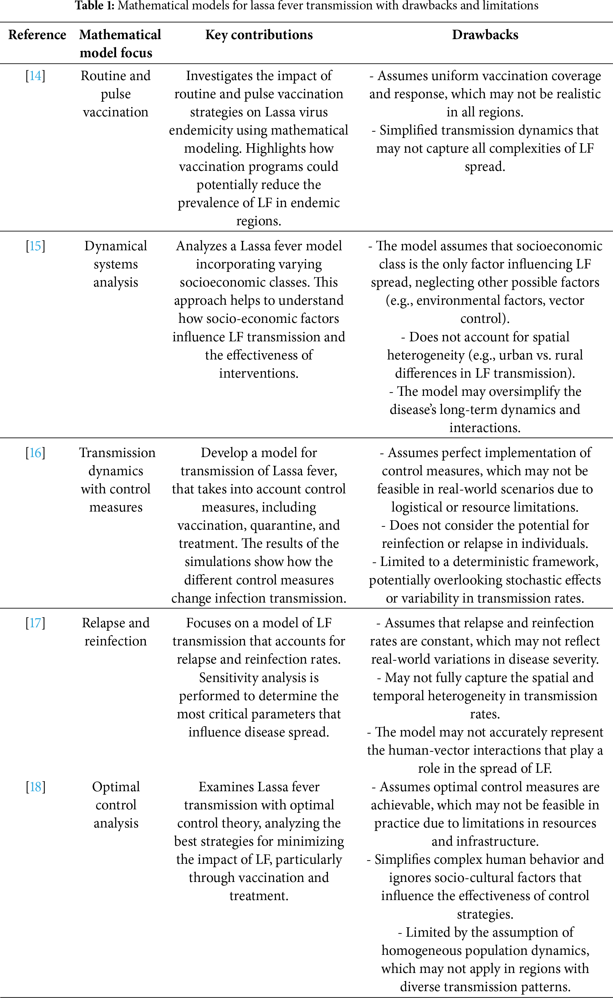
This section provides a review of fundamental concepts related to fractional calculus and its key findings. To capture the drawbacks which are mentioned in Table 1, we incorporated the Caputo fractional derivative into our Lassa Fever model to enhance its accuracy and better capture the complexities of the disease dynamics, and key contributions with limitations of work are also discussed in Table 1.
Definition 1 [35]. Let
Definition 2 [35]. If
where
Lemma 1 [36]. Let
Remark 1. Let
3 Mathematical Fractional Order of Lassa Fever Model
In past years, the dynamics of mathematical modeling of infectious diseases have emerged as a significant influence. This study looks at a fractional-order compartmental model for the new virus LF in Nigeria, focusing on how to keep the disease under control and prevent outbreaks, unlike traditional models that split populations into separate groups of different sizes over time. The paper presents a six-compartment LF model, where
The compartments in the model are described as follows:
• Susceptible Humans
• Exposed Humans
• Infectious Humans
• Recovered Humans
• Susceptible Rodents
• Infectious Rodents
The use of a fractional-order model utilizing the Caputo derivative stems from its effectiveness in accounting for memory effects and long-range interactions that are characteristics of many epidemiological systems, including the transmission of Lassa Fever. The Caputo derivative is used to construct a fractional-order derivative that accommodates non-local effects and long-term dependence associated with the transmission of disease through complicated landscapes. This model is an enhancement over traditional models with the object of supplying better continuance predictions by capturing real-world dynamics. Ojo & Goufo [37] posited the model for LF transmission as follows:
Lassa Fever Model with Fractional Derivative
Epidemics generally have long-term effects, & fractional-order models which can be used to explore these aspects. Fractional-order ‘derivative’, which permits derivatives between
with initial conditions:
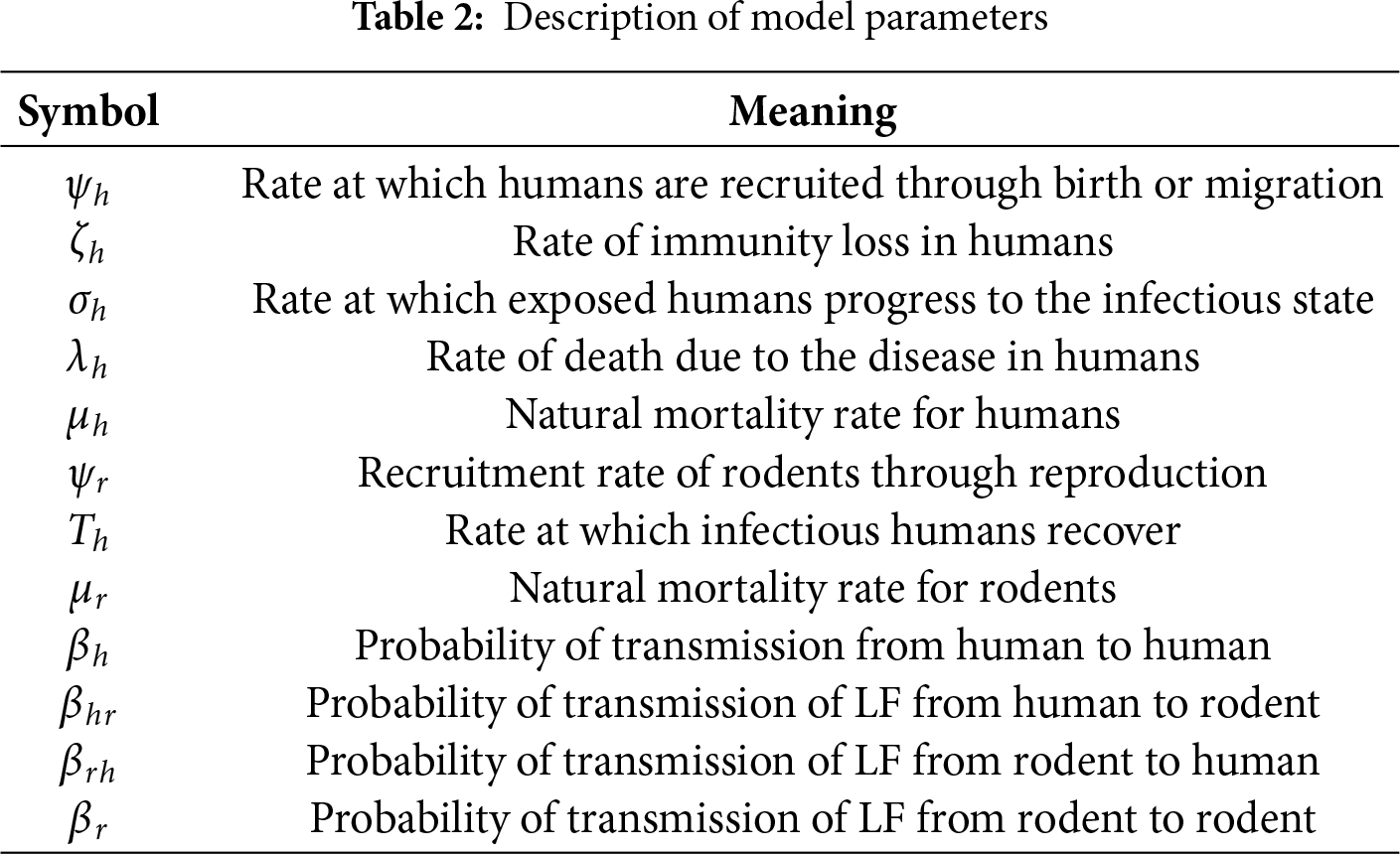
Fig. 1 presents the flow diagram of the dynamical system. The susceptible human population increases at a rate of
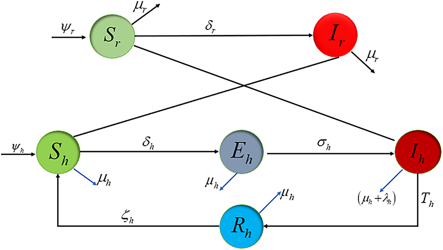
Figure 1: Lassa fever flow sheet
4 Analysis of Proposed Lassa Model
4.1 Positive-Ness and Bounded-Ness of Solutions
A major purpose of this study is to examine the conditions under which LF’s model, whose solution sets must be limited and positive, can be implemented in real-world scenarios. We are aware of the following facts about classical derivatives. The system’s positivity and boundedness are demonstrated through deduced results [38]. We have
we obtain,
Theorem 1. The suggested LF fractional-order model (7) has a unique and bounded solution along the initial conditions (8) in
Proof: Based on model (7), we discover
4.2 Uniqueness and Existence Findings
The fixed point theory approach is utilized to identify the uniqueness of a mathematical model’s solution, revealing the existence of model (7) under specific conditions. The Caputo model (7) acts as the mathematical basis for analyzing the dynamics of the LF disease model, along with feasibility and stability. The sub-sections of the model computed the Lipchitz condition, including existence, uniqueness, and stability of the system.
Let
where
Taking
Let
Setting
For
where
Subsequently Eq. (17) transforms into:
Based on the initial conditions in (8), the difference between successive terms is given as follows:
Let us consider:
Hence, we have the following expressions:
and we obtain the desired relations as follows:
where
Building on the previous analysis, we present and prove the following theorem:
Theorem 2. Assume that the functions
is true for all
Proof. As
after simplification We obtain the following:
As
This guarantees that the suggested model has a solution. To demonstrate that this is a unique solution, we will follow the steps outlined below.
Let a system of solutions to (7) exists, say
where
This leads to the conclusion that
Following a similar approach, similar results can be derived for the remaining compartments.
4.3 Equilibrium Points Analysis
This section aims to provide a detailed review of equilibrium points. To establish the existence of the endemic equilibrium, we need to solve for the steady-state solutions of the system, i.e., the points where the derivatives of all compartments of (7) are zero. We have the following system of equations,
The Lassa fever-free equilibrium point, denoted by
Firstly we consider the system of
Rearrange to solve for
Factor out
Finally, solve for
Now we consider the system of
Rearrange to solve for
Substitute the expression for
The rest of the endemic equilibrium points are computed as follows, which are denoted by
where
In disease epidemiology, the basic reproduction number is a threshold value that determines whether a disease can be controlled. Researchers often use the next-generation matrix approach [37] to calculate this number for biological models. At the disease-free equilibrium (DFE) point, two matrices are considered: F for new infections and V for individual transfer.
LF spreads in populations where
4.5 Stability Analysis of Lassa Model
Here, we concentrate on the stability analysis of the proposed model’s solutions, demonstrating how important system stability is for achieving the expected output and carrying out the proposed system’s intended function.
Theorem 3. If
Proof. We obtained the Jacobian matrix of (7) as follows:
At
The characteristic equation is established by
Thus, we have
Disease-free equilibrium point
Theorem 4. If
Proof. The Jacobian matrix of (7) at endemic equilibrium point
Establishing the characteristic equation, we discover
Therefore, the endemic equilibrium point is LAS (locally asymptotically stable).
Stability plays an important role in control systems, especially in the context of fractional-order systems. The technique expands on the idea that Lyapunov candidate function suggests stability in the LF illness system (7). The paper uses Lyapunov functions to determine critical equilibrium points in the suggested system and control theory, evaluating their asymptotic stability in nonlinear systems without explicitly solving fractional differential equations. The following results correspond to our LF model’s global stability analysis.
Lemma 2. Consider for any
Theorem 5. If
Proof. For
After simplification, we get:
Set
Substituting
Choose
Since
Thus, the disease-free equilibrium is globally asymptotically stable when
5 Computational Analysis Using Fractional Operators
The power law impact was mathematically included into fractional calculus using the Caputo derivative and Newton polynomial interpolation. We proposed a numerical technique for the system (7) using a Newton polynomial [38]. For higher-order interpolation polynomials, Newton’s method offers the benefit of nested multiplication and is relatively easier when adding additional data points compared to Lagrange interpolation. Due to the fact that the Newton polynomial tends to be more accurate than the Lagrange polynomial, which is used in constructing the widely recognized Adams-Bashforth numerical scheme, a numerical scheme based on the Newton polynomial would generally yield greater accuracy than one based on the Lagrange polynomial. Consider
where,
By applying the fractional integral with a power-law kernel, we obtain
Let us examine the Newton polynomial:
Upon simplifying the Newton polynomial and performing further reductions, we derived the final expressions:
Stability in numerical methods is critical because errors are unavoidable in calculations. Stable explicit numerical schemes outperform implicit and linearized schemes in terms of calculation efficiency. The Principle of Mathematical Induction is utilized to demonstrate the unconditional stability and convergence of these schemes. Mathematical induction is a powerful approach for proving general assertions, such as that something is true for all positive integers or from some point forward.
The initial value problem can be expressed as:
The idea of stability in numerical systems refers to minor deviations in numerical solutions produced by perturbations in the initial conditions. Let
Thus, the proposed scheme is stable.
Lemma 3. According to the proposed scheme, the weights will be as follows:
where
Theorem 6. Let the solutions be expressed as:
Proof. Let
holds. Then
From Lemma 3, one can find
The proof can now be concluded using inductive reasoning and mathematical induction
7 Numerical Results and Discussions
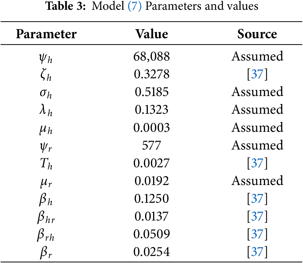
The nonlinear fractional-order Lassa fever has been evaluated through numerical simulations in this section. The stable iterative method discussed in the previous section is verified using a power-law kernel for several fractional orders. The effect of various factors has been evaluated through graphical representations. The study employed numerical simulations with specific element values to assess the impact of the Caputo fractional derivative on the dynamics of the LF disease system. Prior research [37] is used to assess the parametric values for certain assumed values. We evaluated the dynamic behavior of the suggested LF model using the parameter values from Table 3. The fractional-order approach provides the information to capture memory effect and hereditary qualities inherent in the LF disease dynamics, as well as deeper insights into the system’s temporal history. By altering the fractional-order
The numerical simulation for different fractional values are illustrated by examining steady-state behavior with the Caputo derivative. Figs. 2–7 illustrate approximate solutions for different fractional orders. Fig. 2 depicts the dynamics of the susceptible human population at various fractional orders
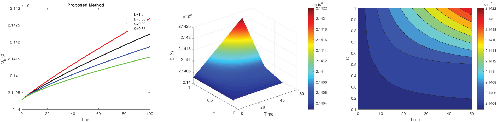
Figure 2: Simulation of
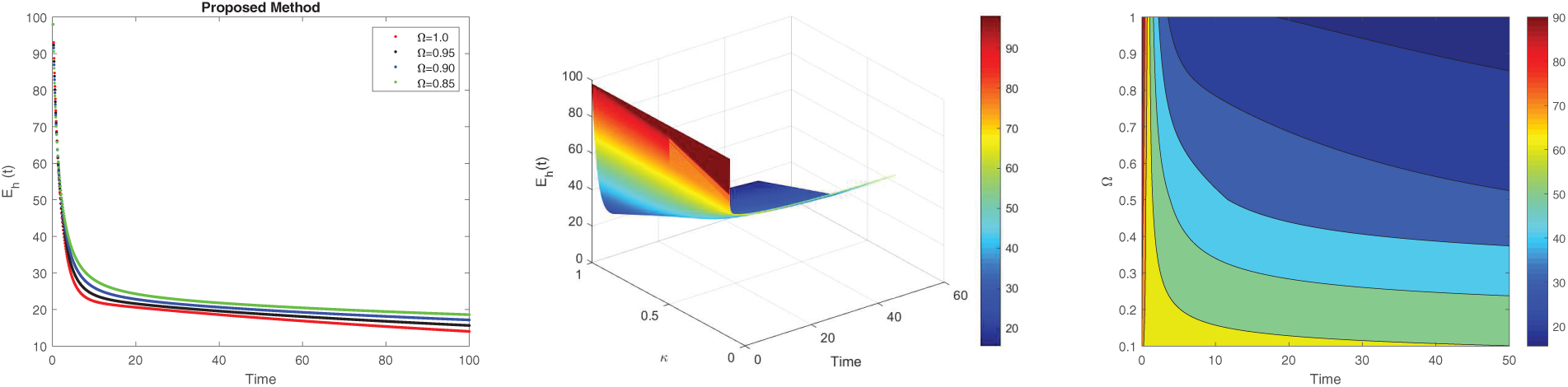
Figure 3: Simulation of
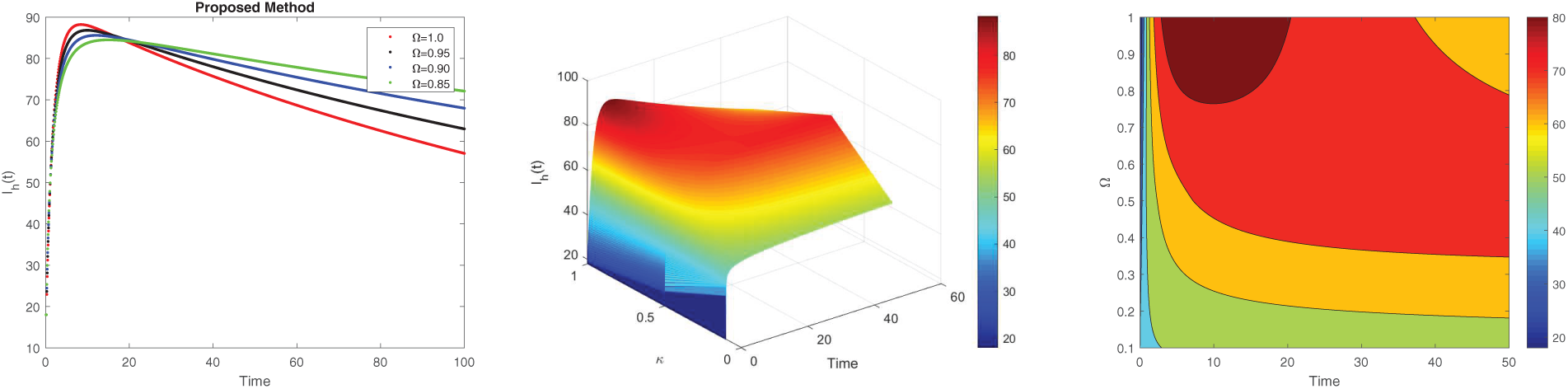
Figure 4: Simulation of
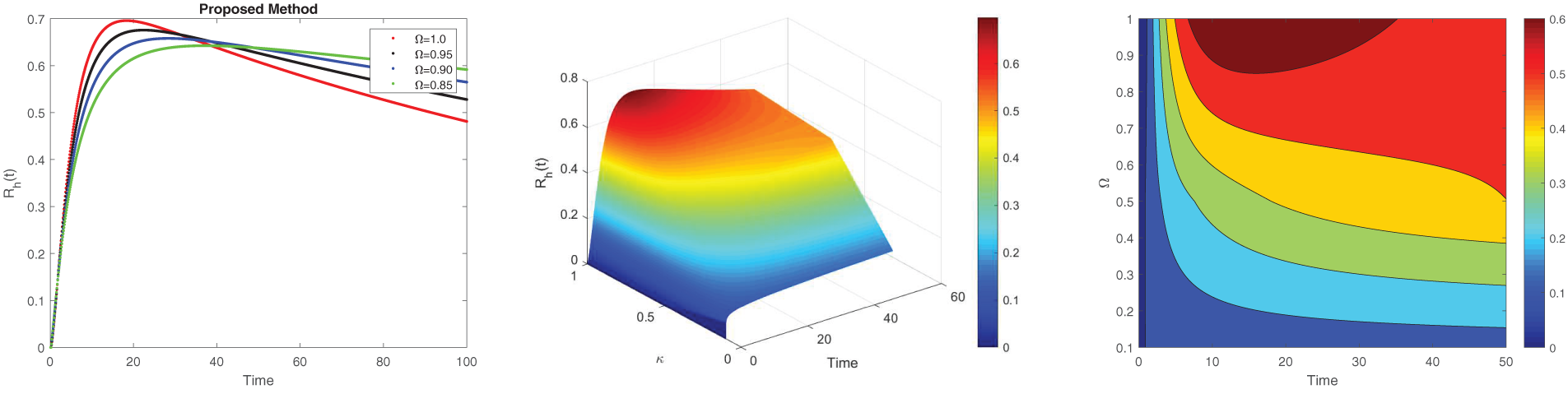
Figure 5: Simulation of
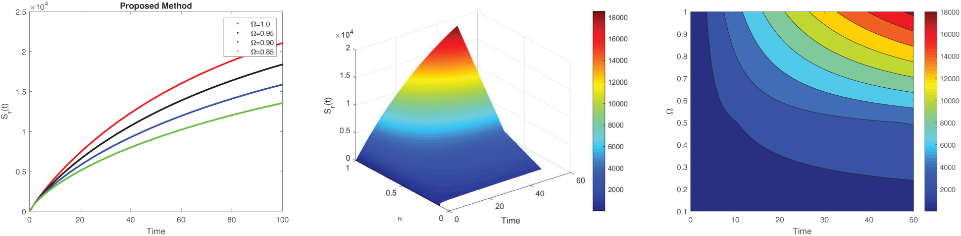
Figure 6: 2D and 3D surface analysis of susceptible for the dynamics of LF with different values of fractional derivatives
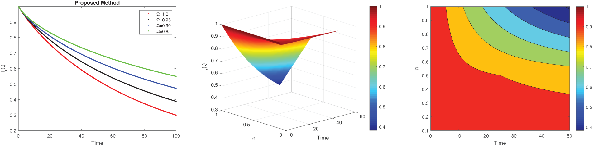
Figure 7: 2D and 3D surface analysis of susceptibility for the dynamics of LF with different values of fractional derivatives
Fig. 4 displays the dynamics of the infected human population for various fractional orders. In Fig. 4a, it is evident that the number of infected individuals increases noticeably as the fractional order
Fig. 5 depicts the recovery dynamics pattern of the human for several fractional orders. Fig. 5a shows that as
Fig. 6 demonstrates the dynamic pattern of the susceptible rodent across different fractional orders
Fig. 7 presents the dynamic pattern of the infected rodent for several fractional orders. Panel 7a shows that the infected rodents decrease significantly as
The non-local nature of the Caputo operator emphasizes the influence of memory on the dynamics of Lassa fever transmission. Across all figures, the solutions converge to a steady state within the bounded region for different fractional order values, demonstrating the stabilizing effect of fractional dynamics in the system. To compare the integer and non-integer-order models, we use the typical integer-order solution at
Figs. 8–13 present the sensitivity surface plots for
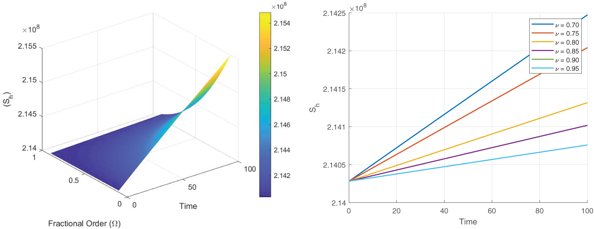
Figure 8: Sensitivity surface plot of
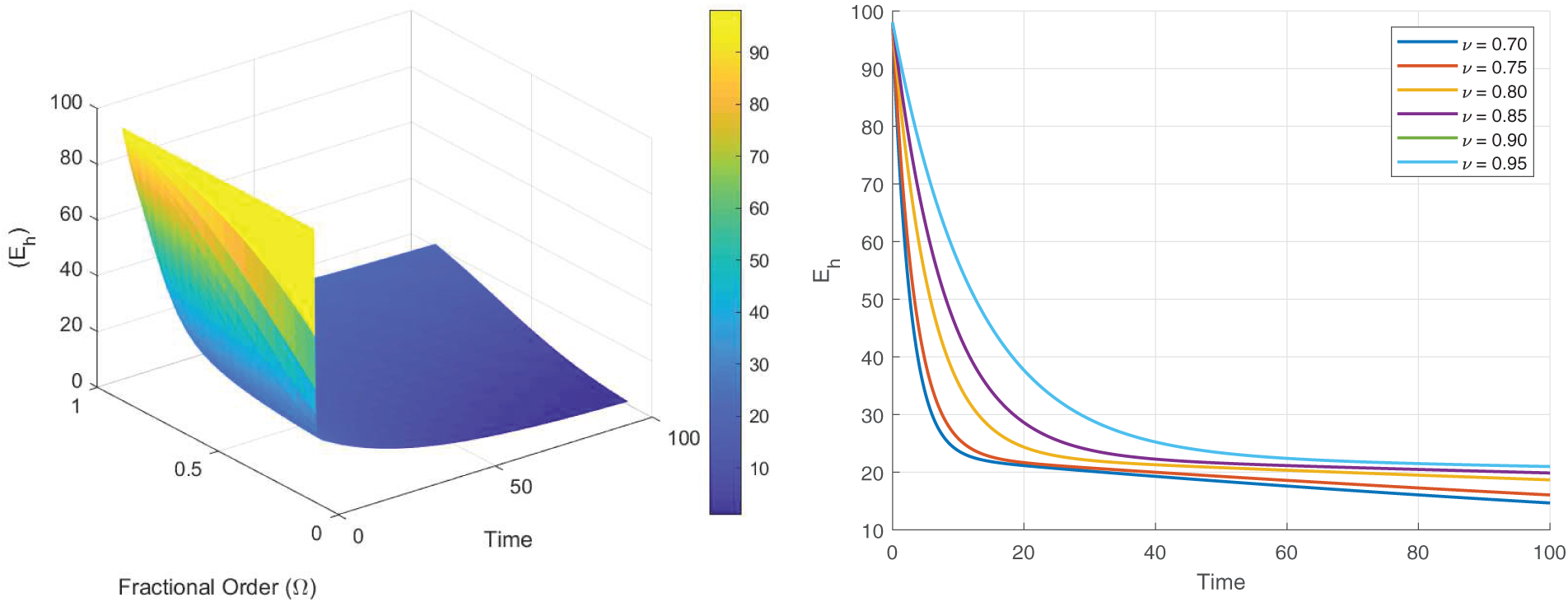
Figure 9: Sensitivity surface plot of
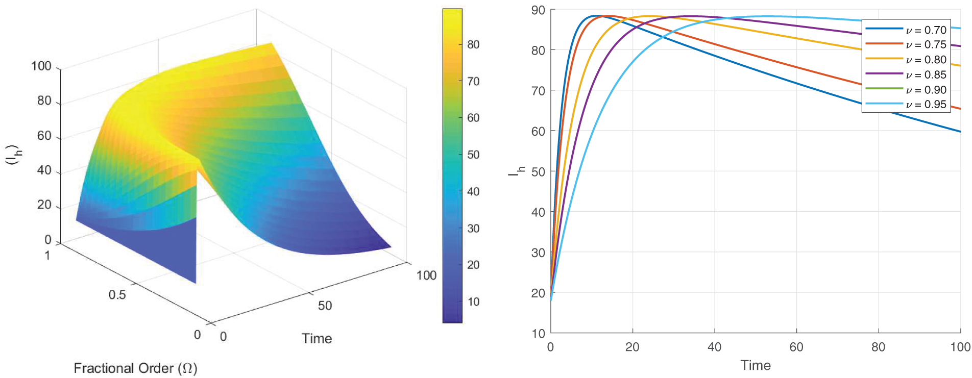
Figure 10: Sensitivity surface plot of
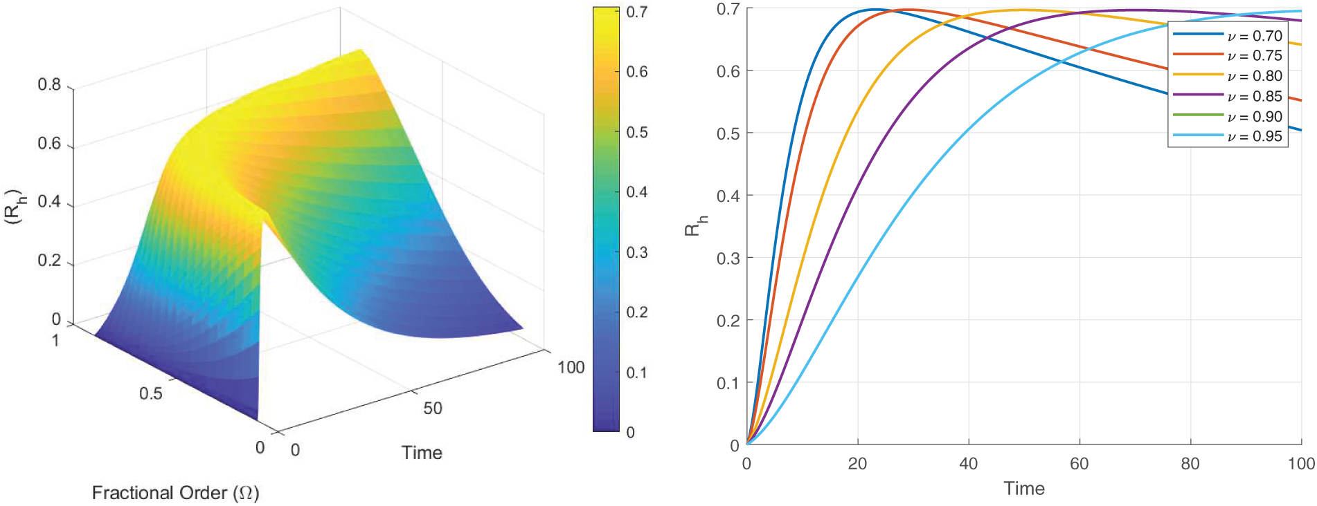
Figure 11: Sensitivity surface plot of
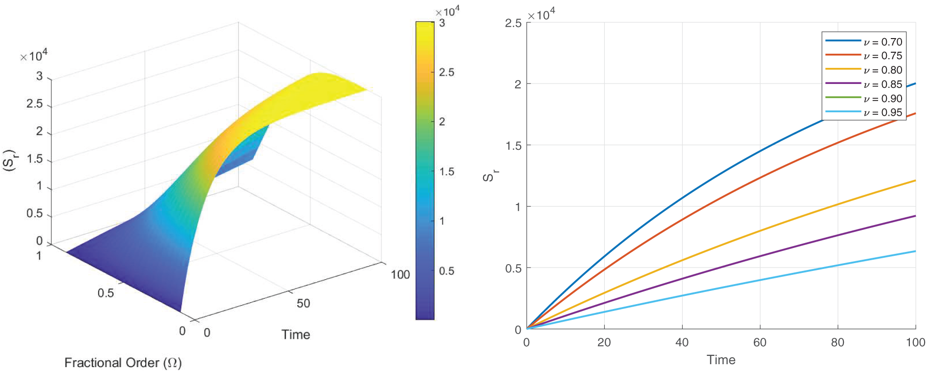
Figure 12: Sensitivity surface plot of
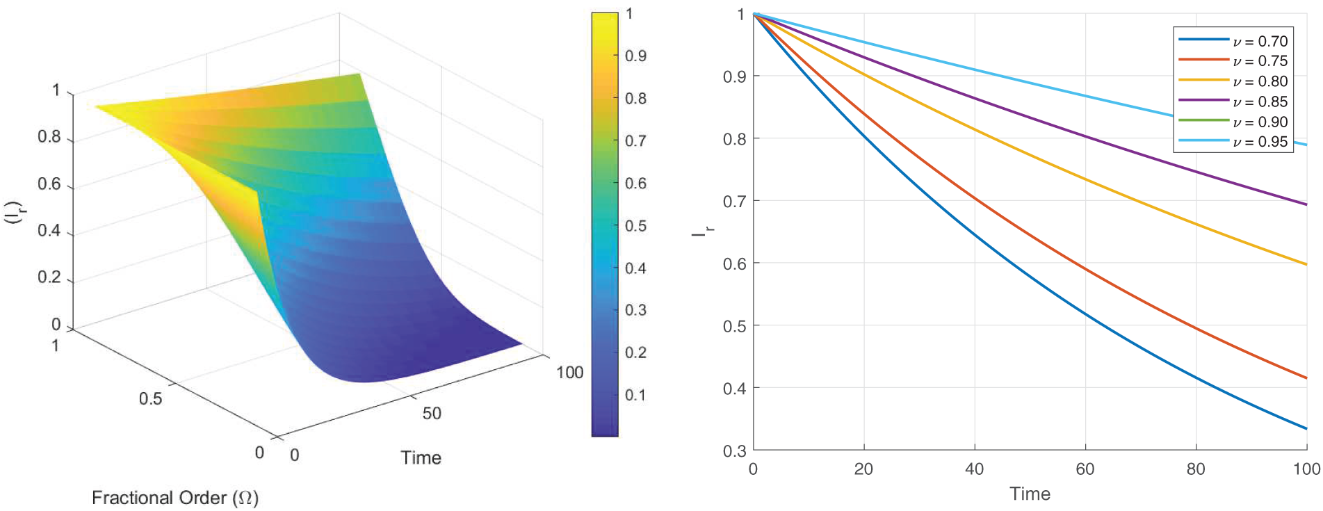
Figure 13: Sensitivity surface plot of
A nonlinear compartmental model was presented in this study that models the transmission dynamics of Lassa fever (LF) by dividing the population into four mutually exclusive compartments. The nonlinear fractional-order differential equations in the model have been proven well-posed. Furthermore, the system is bounded and stays in the positive region throughout the simulation, which guarantees that all state variables have biological meanings and properties that are proven in this work. Global asymptotic stability of the system was also determined using the Lyapunov function. A more thorough qualitative analysis was performed to identify the model equilibrium points and reproductive number as an important measure of the risk of an epidemic. This statistic indicates the extent to which LF transmits through the population, offering valuable information for public health management. The sensitivity analysis identified the parameters that most affect transmission dynamics; these parameters may be targets for effective intervention strategies. The Newton polynomial interpolation method was implemented to account for incremental data, which produces a sequence of higher-degree polynomials that increases the accuracy of the function approximating values on the interval of interest. This method allows calculations to be performed much more efficiently while avoiding reevaluating results that would otherwise be repeated in several scenarios, which is useful for complex simulations using random processes. We performed numerical simulations to examine the effects of various factors on LF severity and progression. We found that Caputo methodology using fractional-order methods is more effective than the traditional methods, reported new results that contribute to creating the intervention framework, and that the Caputo order is able to keep track of invasive or traditional methods that would typically require modeling complex dynamics between humans and rodents. While this study contributes to some understanding of LF control and transmission, the low amount of available real-world findings limits the applicability of the results. The key takeaway from this research is that there is a clear need for strong surveillance systems that may enable us to respond quickly and administer antiviral therapy, which can have a big impact on the reduction of LF transmission and loss of life. Methods addressing the reduction of human-rodent interaction, such as household sanitation, food storage in rodent-proof containers, should also be used in affected areas. However, our work also provides an important theoretical and computational framework for future studies, as well as offers a basis for policy-makers to help create interventions. It would be beneficial to study alternative mathematics frameworks, such as Stochastic fractional derivatives, and look at a robust dataset to enhance predictive power and to its application field using Neural Network (NN) and Physics Informed Neural Network (PINN).
Acknowledgement: None.
Funding Statement: The authors received no specific funding for this study.
Author Contributions: The contributions of each author to this research are as follows: Conceptualization, Muhammad Farman, Mohamad Hashir Zubair and Kottakkaran Sooppy Nisar; methodology, Muhammad Farman, Hua Li and Kottakkaran Sooppy Nisar; software, Muhammad Farman and Mohamad Hashir Zubair; validation, Hua Li and Mohamad Hafez; formal analysis, Kottakkaran Sooppy Nisar; investigation, Muhammad Farman, Mohamad Hashir Zubair and Kottakkaran Sooppy Nisar; resources, Mohamad Hafez; data curation, Mohamad Hafez; writing—original draft preparation, Muhammad Farman and Mohamad Hafez Zubair; writing—review and editing, Muhammad Farman, Mohamad Hashir Zubair, Kottakkaran Sooppy Nisar; visualization, Muhammad Farman and Hua Li; supervision, Muhammad Farman and Hua Li; project administration, Muhammad Farman. All authors reviewed the results and approved the final version of the manuscript.
Availability of Data and Materials: All data analyzed and generated during this study are included in this article.
Ethics Approval: Not applicable.
Conflicts of Interest: The authors declare no conflicts of interest to report regarding the present study.
References
1. Peterson AT, Moses LM, Bausch DG. Mapping transmission risk of Lassa fever in West Africa: the importance of quality control, sampling bias, and error weighting. PLoS One. 2014;9(8):e100711. doi:10.1371/journal.pone.0100711. [Google Scholar] [PubMed] [CrossRef]
2. Ibrahim MA, Dénes A. A mathematical model for Lassa fever transmission dynamics in a seasonal environment with a view to the 2017–2020 epidemic in Nigeria. Nonlinear Anal Real World Appl. 2021;60:103310. doi:10.1016/j.nonrwa.2021.103310. [Google Scholar] [CrossRef]
3. Zhao S, Musa SS, Fu H, He D, Qin J. Large-scale Lassa fever outbreaks in Nigeria: quantifying the association between disease reproduction number and local rainfall. Epidemiol Infect. 2020;148:e4. doi:10.1017/S0950268819002267. [Google Scholar] [PubMed] [CrossRef]
4. Gibb R, Moses LM, Redding DW, Jones KE. Understanding the cryptic nature of Lassa fever in West Africa. Pathog Glob Health. 2017;111(6):276–88. doi:10.1080/20477724.2017.1369643. [Google Scholar] [PubMed] [CrossRef]
5. Richmond JK, Baglole DJ. Lassa fever: epidemiology, clinical features, and social consequences. BMJ. 2003;327(7426):1271–5. doi:10.1136/bmj.327.7426.1271. [Google Scholar] [PubMed] [CrossRef]
6. Greenky D, Knust B, Dziuban EJ. What pediatricians should know about Lassa virus. JAMA Pediatr. 2018;172(5):407–8. doi:10.1001/jamapediatrics.2017.5223. [Google Scholar] [PubMed] [CrossRef]
7. Mariën J, Borremans B, Kourouma F, Baforday J, Rieger T, Günther S, et al. Evaluation of rodent control to fight Lassa fever based on field data and mathematical modelling. Emerg Microbes Infect. 2019;8(1):640–9. doi:10.1080/22221751.2019.1605846. [Google Scholar] [PubMed] [CrossRef]
8. Olugasa BO, Odigie EA, Lawani M, Ojo JF. Development of a time-trend model for analyzing and predicting case-pattern of Lassa fever epidemics in Liberia, 2013–2017. Ann Afr Med. 2015;14(2):89–96. doi:10.4103/1596-3519.149892. [Google Scholar] [PubMed] [CrossRef]
9. Musa SS, Zhao S, Gao D, Lin Q, Chowell G, He D. Mechanistic modelling of the large-scale Lassa fever epidemics in Nigeria from 2016 to 2019. J Theor Biol. 2020;493(1):110209. doi:10.1016/j.jtbi.2020.110209. [Google Scholar] [PubMed] [CrossRef]
10. Hamblion EL, Raftery P, Wendland A, Dweh E, Williams GS, George RN, et al. The challenges of detecting and responding to a Lassa fever outbreak in an Ebola-affected setting. Int J Infect Dis. 2018;66(6):65–73. doi:10.1016/j.ijid.2017.11.007. [Google Scholar] [PubMed] [CrossRef]
11. Asogun DA, Günther S, Akpede GO, Ihekweazu C, Zumla A. Lassa fever: epidemiology, clinical features, diagnosis, management and prevention. Infect Dis Clin. 2019;33(4):933–51. doi:10.7759/cureus.28598. [Google Scholar] [CrossRef]
12. Maxmen A. Deadly Lassa-fever outbreak tests Nigeria’s revamped health agency. Nature. 2018;555(7697):421–3. doi:10.1038/d41586-018-03171-y. [Google Scholar] [CrossRef]
13. Dalhat MM, Olayinka A, Meremikwu MM, Dan-Nwafor C, Iniobong A, Ntoimo LF, et al. Epidemiological trends of Lassa fever in Nigeria, 2018–2021. PLoS One. 2022;17(12):e0279467. doi:10.1371/journal.pone.0279467. [Google Scholar] [PubMed] [CrossRef]
14. Davies J, Lokuge K, Glass K. Routine and pulse vaccination for Lassa virus could reduce high levels of endemic disease: a mathematical modelling study. Vaccine. 2019;37(26):3451–6. doi:10.1016/j.vaccine.2019.05.010. [Google Scholar] [PubMed] [CrossRef]
15. Onah IS, Collins OC. Dynamical system analysis of a Lassa fever model with varying socioeconomic classes. J Appl Math. 2020;2020(1):2601706. doi:10.1155/2020/2601706. [Google Scholar] [CrossRef]
16. Idisi OI, Yusuf TT. A mathematical model for lassa fever transmission dynamics with impacts of control measures: analysis and simulation. Eur J Math. 2021;2(2):19–28. doi:10.24018/ejmath.2021.2.2.17. [Google Scholar] [CrossRef]
17. Erinle-Ibrahim LM, Adebimpe O, Lawal WO, Agbomola JO. A mathematical model and sensitivity analysis of Lassa fever with relapse and reinfection rate. Tanz J Sci. 2022;48(2):414–26. doi:10.4314/tjs.v48i2.16. [Google Scholar] [CrossRef]
18. Peter OJ, Abioye AI, Oguntolu FA, Owolabi TA, Ajisope MO, Zakari AG, et al. Modelling and optimal control analysis of Lassa fever disease. Inform Med Unlocked. 2020;20:100419. doi:10.1016/j.imu.2020.100419. [Google Scholar] [CrossRef]
19. Rashid S, Jarad F. Novel investigation of stochastic fractional differential equations measles model via the white noise and global derivative operator depending on mittag-leffler kernel. Comput Model Eng Sci. 2024;139(3):2289–327. doi:10.32604/cmes.2023.028773. [Google Scholar] [CrossRef]
20. Hafez M, Alshowaikh F, Voon BWN, Alkhazaleh S, Al-Faiz H. Review on recent advances in fractional differentiation and its applications. Prog Fract Differ Appl. 2025;11(2):245–61. doi:10.18576/pfda/110203. [Google Scholar] [CrossRef]
21. Farman M, Gokbulut N, Hurdoganoglu U, Hincal E, Suer K. Fractional order model of MRSA bacterial infection with real data fitting: computational Analysis and Modeling. Comput Biol Med. 2024;173(3):108367. doi:10.1016/j.compbiomed.2024.108367. [Google Scholar] [PubMed] [CrossRef]
22. Farman M, Akgül A, Hashemi MS, Guran L, Bucur A. Fractal fractional order operators in computational techniques for mathematical models in epidemiology. Comput Model Eng Sci. 2024;138(2):1385–1403. doi:10.32604/cmes.2023.028803. [Google Scholar] [CrossRef]
23. Farman M, Hincal E, Jamil S, Gokbulut N, Nisar KS, Sambas A. Sensitivity analysis and dynamics of brucellosis infection disease in cattle with control incident rate by using fractional derivative. Sci Rep. 2025;15(1):355. doi:10.1038/s41598-024-83523-z. [Google Scholar] [PubMed] [CrossRef]
24. Abdullahi A. Modelling of transmission and control of Lassa fever via Caputo fractional-order derivative. Chaos Solit. 2021;151:111271. doi:10.1016/j.chaos.2021.111271. [Google Scholar] [CrossRef]
25. Ali A, ur Rahman M, Arfan M, Shah Z, Kumam P, Deebani W. Investigation of time-fractional SIQR Covid-19 mathematical model with fractal-fractional Mittage-Leffler kernel. Alex Eng J. 2022;61(10):7771–9. doi:10.1016/j.aej.2022.01.030. [Google Scholar] [CrossRef]
26. Chu Y-M, Rashid S, Sultana S, Inc M. New numerical simulation for the fractal-fractional model of deathly lassa hemorrhagic fever disease in pregnant women with optimal analysis. Fractals. 2023;31(4):2340054. doi:10.1142/S0218348X23400546. [Google Scholar] [CrossRef]
27. Ghanbari B, Kumar S. A study on fractional predator-prey-pathogen model with Mittag-Leffler kernel-based operators. Numer Meth Part Differ Equ. 2024;40(1):e22689. doi:10.1002/num.22689. [Google Scholar] [CrossRef]
28. Rashid S, Karim S, Akgül A, Bariq A, Elagan SK. Novel insights for a nonlinear deterministic-stochastic class of fractional-order Lassa fever model with varying kernels. Sci Rep. 2023;13(1):15320. doi:10.1038/s41598-023-42106-0. [Google Scholar] [PubMed] [CrossRef]
29. Zhang L, ur Rahman M, Arfan M, Ali A. Investigation of mathematical model of transmission co-infection TB in HIV community with a non-singular kernel. Results Phys. 2021;28:104559. doi:10.1016/j.rinp.2021.104559. [Google Scholar] [CrossRef]
30. Farman M, Alfiniyah C, Saqib M. Global stability with lyapunov function and dynamics of SEIR-modified lassa fever model in sight power law kernel. Complex. 2024;2024(1):3562684. doi:10.1155/2024/3562684. [Google Scholar] [CrossRef]
31. Kumar S, Chauhan RP, Momani S, Hadid S. Numerical investigations on COVID-19 model through singular and non-singular fractional operators. Numer Meth Part Differ Equ. 2024;40(1):e22707. doi:10.1002/num.22707. [Google Scholar] [CrossRef]
32. Abidemi A, Owolabi KM. Unravelling the dynamics of Lassa fever transmission with nosocomial infections via non-fractional and fractional mathematical models. Eur Phys J Plus. 2024;139(2):1–30. doi:10.1140/epjp/s13360-024-04910-z. [Google Scholar] [CrossRef]
33. Kumar S, Kumar A, Samet B, Dutta H. A study on fractional host-parasitoid population dynamical model to describe insect species. Numer Meth Part Differ Equ. 2021;37(2):1673–92. doi:10.1002/num.22603. [Google Scholar] [CrossRef]
34. Ahmad S, Ullah A, Riaz MB, Ali A, Akgül A, Partohaghighi M. Complex dynamics of multi strain TB model under nonlocal and nonsingular fractal fractional operator. Results Phys. 2021;30:104823. doi:10.1016/j.rinp.2021.104823. [Google Scholar] [CrossRef]
35. Li C, Qian D, Chen Y. On Riemann-Liouville and caputo derivatives. Discrete Dyn Nature Soc. 2011;2011(1):562494. doi:10.1155/2011/562494. [Google Scholar] [CrossRef]
36. Alkahtani BS, Alzaid SS. Studying the dynamics of the rumor spread model with fractional piecewise derivative. Symmetry. 2023;15(8):1537. doi:10.3390/sym15081537. [Google Scholar] [CrossRef]
37. Ojo MM, Goufo EF. Modeling, analyzing and simulating the dynamics of Lassa fever in Nigeria. J Egypt Math Soc. 2022;30(1):1. doi:10.1186/s42787-022-00138-x. [Google Scholar] [CrossRef]
38. Atangana A. Mathematical model of survival of fractional calculus, critics and their impact: how singular is our world. Adv Differ Equ. 2021;2021(1):403. doi:10.1186/s13662-021-03494-7. [Google Scholar] [CrossRef]
Cite This Article
 Copyright © 2026 The Author(s). Published by Tech Science Press.
This work is licensed under a Creative Commons Attribution 4.0 International License , which permits unrestricted use, distribution, and reproduction in any medium, provided the original work is properly cited.
 Downloads
 Citation Tools