Multivariate Data Anomaly Detection Based on Graph Structure Learning

1  Introduction

Multivariate data refer to data obtained by simultaneously collecting multiple variables (attributes or features) from the same observed entity. Each variable represents a specific dimension of information, and multivariate data can help reveal the relationships or interactions among these dimensions. With the increasing complexity of information systems, the acquisition of multivariate data has become a critical requirement. Typically, information systems employ physical or virtual devices (e.g., temperature sensors, barcodes, or logging points) to collect data from different components or functional modules, thereby reflecting the operational state of the system [1]. Such data are widely used in practical scenarios including operations monitoring, anomaly detection, and system optimization.

However, the collection of operational monitoring data in information systems is influenced by multiple factors, such as deployment environments, hardware performance, and network stability. These factors may introduce temporal inconsistencies in the collected data, which severely compromise the effectiveness of anomaly detection. We refer to this phenomenon as multivariate temporal dependency misalignment. Conventional anomaly detection algorithms may misinterpret temporal patterns across variables, thereby undermining the generalization and robustness of the models.

In recent years, multivariate data anomaly detection has been widely applied in fields such as industrial manufacturing, financial transactions, and network security [2,3]. However, existing studies have largely overlooked the modeling of inter-variable couplings under misaligned temporal sequences, making it difficult to address sudden and high-intensity structural perturbations during system operation. To address this challenge, researchers have introduced graph neural networks (GNNs) to more effectively capture structural couplings among variables [4]. In GNNs, multivariate data are represented as a graph. Each node corresponds to a variable, and edges encode the strength of inter-variable dependencies, enabling effective modeling of structural relationships. However, most existing approaches either rely on static graphs [5] or construct graph structures using predefined correlation coefficients [6], which makes them insufficiently adaptive to time-varying inter-variable dependencies. This limitation is particularly pronounced in environments with temporal misalignment, where their ability to model structural dependencies degrades significantly.

To address these challenges, we propose a multivariate data anomaly detection model under graph structure learning (GSL-AD), which leverages graph structures to enhance the representation of the spatial relationships within multivariate data and reduce the reliance on temporal features. Firstly, the initial graph structure of the multivariate coupled network is constructed based on a recommendation strategy, and the edge weights of this graph are optimized using a multi-channel graph encoding layer. Secondly, through a multi-stage feature compressor, the structural and embedding features of the optimized graph are extracted, followed by joint optimization based on both reconstruction and prediction. Finally, reconstruction and prediction errors are employed as anomaly scores for anomaly detection. An unsupervised approach to anomaly detection, along with anomaly structure visualization and diagnostic research, is carried out using a dynamic threshold selection algorithm based on extreme value theory.

The main contributions of this study are as follows:

1.    We propose a graph structure learning-based framework for multivariate anomaly detection, termed GSL-AD. In this framework, a recommendation strategy is introduced during the construction of the initial graph, and edge weights are adaptively optimized through a multi-channel graph attention encoder, enabling the model to capture both spatial dependencies and latent dynamic changes among variables. Subsequently, a multi-stage feature compressor is employed to jointly extract structural and embedding features, and joint optimization based on reconstruction and prediction is applied to achieve robust modeling of misaligned dependencies.

2.    An anomaly scoring mechanism based on reconstruction and prediction errors is proposed, along with a dynamic thresholding strategy derived from extreme value theory, enabling fully unsupervised anomaly detection. The optimized graph structure is also utilized for anomaly visualization and structural perturbation analysis, providing intuitive insights for diagnosing the causes of anomalies.

3.    Experimental results on multiple public datasets and industrial scenarios suggest that the proposed method tends to perform better than existing mainstream methods in terms of mean AUC, recall, precision, and F1 score.

2  Related Work

In recent years, significant advances have been achieved in multivariate data anomaly detection. Broadly, current methods fall into five categories: statistical approaches, clustering approaches, density-based approaches, deep learning approaches, and graph neural network approaches.

Statistical techniques are the mainstay of early approaches, which model data distributions (e.g., Gaussian or Poisson) and identify anomalies as low-probability events [7,8]. However, these methods are often inadequate for real-world systems with unknown or inherently complex underlying mechanisms. With the progress of technology, a variety of anomaly detection approaches have emerged, including those based on distance, clustering, density, or graph structures.

Multivariate anomaly detection methods that rely on distance measures consider data points with significantly larger distances from their neighbors as anomalies [9]. For example, Qiu et al. [10] construct a multivariate anomaly detection model using Principal Component Analysis, where anomalies are detected by comparing the distances between normal and abnormal data points. Multivariate anomaly detection methods that utilize clustering techniques regard normal data as forming well-defined clusters, while anomalous points are those that do not associate with any cluster. Anomalies are identified by evaluating the degree of association between each data point and the identified clusters. For example, Li et al. [11] apply an extended fuzzy clustering algorithm to fit the latent structures in multivariate data and to detect anomalies in both amplitude and shape. Tan and Yiu [12] improve the accuracy of anomaly detection by optimizing the clustering process through parameter adaptation. Another common approach to multivariate anomaly detection involves analyzing the distribution of local data densities, which is based on the assumption that anomalies tend to occur in sparsely populated regions. For instance, Breunig et al. [13] and Cheng et al. [14] detect anomalies by comparing the local density of each data point with that of its neighbors. A point is likely to be identified as anomalous if it exhibits low local density while the surrounding points demonstrate relatively high densities.

Although deep learning methods are relatively simple and easy to generalize, they often struggle to effectively capture the complex and diverse nonlinear relationships among multiple variables in multivariate data. As a result, more sophisticated approaches are required to accurately identify and interpret anomalies in such data. Graph-structured approaches represent multivariate data as graphs and optimize edge weights using Graph Neural Networks (GNNs), thereby providing extended information for anomaly detection methods based on prediction or reconstruction. Currently, in the field of anomaly detection based on multivariate coupled networks, Wang et al. [15], Silva [16] and Sun et al. [17] employ GNNs [18] to optimize edge weights within the network structure, thereby overcoming the limitations of traditional machine learning models in capturing the complex relationships among variables. In addition, the visualization of anomalous nodes in the multivariate coupled network structure facilitates the analysis of the underlying causes of anomalies. In related studies on anomaly detection based on multivariate coupled networks [2,19–21], a sliding window sampling strategy is commonly employed to generate temporally correlated sequence segments, which are then used as embedded features of the initial graph nodes. However, the occurrence of anomalies in multivariate data is often abrupt in real-world environments, such as power outages, system crashes and other causes. These anomalies are weakly correlated with the historical state changes of the observed data. The mixing of noise data leads to a gradual decline in the generalization performance of the multivariate coupled network structure.

In recent years, research on graph-structured approaches for multivariate time-series anomaly detection has further deepened. The GDN model proposed in [20] characterizes dependencies between variables using a graph structure based on static similarity, but it struggles to adaptively capture dynamic coupling features. In contrast, the OmniAnomaly model introduced in [22] employs a variational autoencoder combined with recurrent neural networks to model temporal dependencies. Although it exhibits strong generalization, it lacks explicit modeling of structural relationships. The Correlation-Aware ST-GNN model presented in [4] incorporates spatio-temporal graph neural networks to enhance correlation modeling, but the strong coupling between structural learning and temporal modeling affects interpretability and generalization performance. Moreover, Khan et al. [23] propose a topology-based anomaly detection framework using graph attention networks (GAT). By integrating substructure analysis and data augmentation, the framework achieves robustness in detecting structural anomalies. Their study shows that incorporating an attention mechanism helps adaptively assign weights to node dependencies, thereby enhancing the model’s ability to represent complex topological anomalies. In this work, we adopt graph structures to represent multivariate coupling relationships. We construct an initial graph through a recommendation strategy and adaptively optimize it using a multi-channel graph attention encoder. At the same time, a multi-stage feature compressor collaboratively extracts structural and embedding features to enhance structural modeling capabilities. Under an unsupervised framework, we integrate reconstruction and prediction tasks to improve detection accuracy and anomaly interpretability, providing a reference for multivariate data anomaly detection in related fields.

3  Multivariate Data Anomaly Detection Model

3.1 Problem Definition

To describe the multivariate coupled network structure constructed through recommendation mechanisms, we offer the following definitions.

Theorem 1: (Initial Graph): Let the initial graph be defined as G=(V,E,X), where V={v1,v2,…,vi} denotes the set of nodes, with i∈RM and M representing the number of variables. The edge set E={e11,e12,…,eij}, where i,j∈RM, encodes pairwise connections among nodes. Each edge eqr=(vq,vr) captures a potential coupling relationship between node vq and node vr. The matrix X contains the embedding features associated with the nodes.

Theorem 2: (Adjacency Matrix): The adjacency matrix A∈RM×M represents the topology of the multivariate coupling network. For example, if there is a connection between nodes vq and vr, then the element Aqr=1; if no connection exists between nodes vq and vr, then Aqr=0.

Theorem 3: (Anomaly Detection): Given a multivariate time series X∈RT×W×M, where T denotes the number of time steps, W the sampling window length, and M the number of variables, the objective of anomaly detection is to learn a mapping that assigns each feature vector xt at time step t to an anomaly score∈R. Based on a predefined or learned threshold γ, each sample is then classified as either normal or anomalous. Anomalies are typically defined as points that deviate from normal patterns in the feature space or structural space.

3.2 Framework Overview

The overall framework of GSL-AD is illustrated in Fig. 1. GSL-AD consists of four modules: the initial graph construction module, the graph structure optimization module, the node feature enhancement module, and the anomaly scoring module. For the input data, the sampling data within a sliding window of length W prior to time step i is used as the input for the initial graph construction. To account for the temporal misalignment effects of multivariate dependencies, we set W=1 and construct the initial graph for each time step i. Subsequently, the weights of multivariate coupling relationships in the initial graph are optimized using a Multi-Channel Graph Attention Layer (MC-GAL). In addition, a multi-channel compressor is employed to compress the topological features of the multivariate coupling network, thereby enhancing the quality of its low-dimensional structural representations. Furthermore, a single-channel self-attention mechanism is applied to improve the representation of critical variable features. Finally, the anomaly score is obtained by taking a weighted average of the prediction-based and reconstruction-based values. Afterward anomalous data points are identified according to this score. The proposed algorithm is detailed as follows.

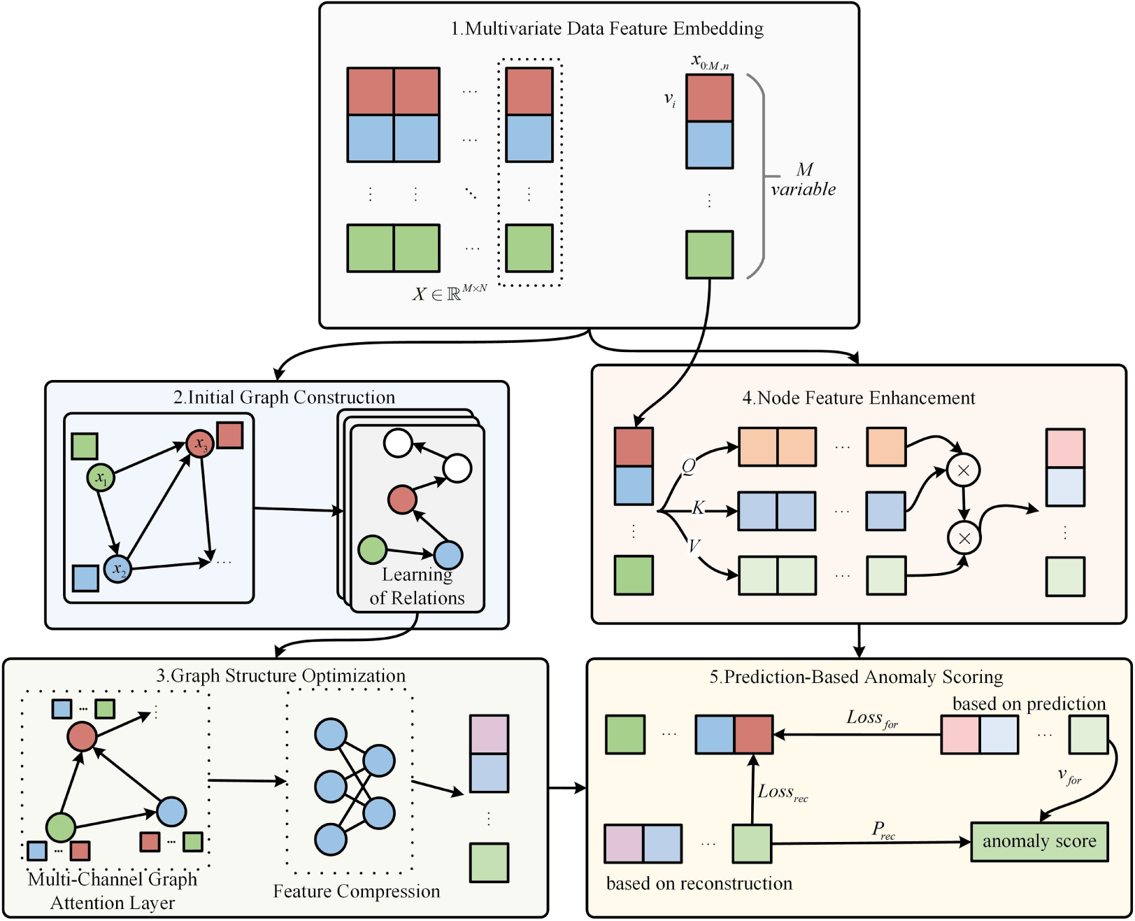
Figure 1: Anomaly detection framework for graph structure learning

3.3 Construction of the Initial Graph for the Multivariate Coupling Network

Since anomalies are often caused by strong interactions among highly coupled variables, we measure the differences between variables using a distance metric. A Top-K strategy is then employed to select the desired level of sparsity by varying the value of K, thereby constructing the initial graph for the multivariate data. This graph serves as the foundational structure of the multivariate coupling network. The construction process of the initial graph is illustrated in Fig. 2.

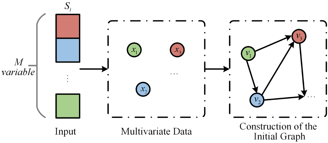
Figure 2: Construction of the initial graph for multivariate data

Based on the sampled data Si, this study constructs the initial graph Gi and the corresponding node embedding features Xi=Si. Eq. (1) defines the node embeddings in the initial graph, where the embedding of each node vii corresponds to elements of Si.

vii=xii∈R1,i∈{1,2,⋯,M}(1)

After constructing the initial graph, we dynamically learn the dependencies among multiple variables, where each node represents a variable and each edge represents a relationship between nodes. The multivariate dependencies in graph Gi are represented by an adjacency matrix Ai, where Aqri indicates an association between nodes vqi and vri. Since multivariate data typically lacks inherent graph structure, we construct prior information by establishing relationships between variable xci and other variables, which serve as candidate relations Cci for variable vci, as shown in Eq. (2). When prior information is unavailable, all variables except vci are considered as candidate relations for vci.

Cci⊆{x1i,xci,⋯,xji},c≠j,j∈RM(2)

Eci={ecji∣ecji=σ(‖xci−xji‖2),j∈Cc}(3)

Eq. (3) is used to compute the dependency relationships between node vci and other nodes, where ‖⋅‖2 denotes the L2 norm representation of the Minkowski distance, and ecji represents the degree of association between node vci and node vji within the i-th sliding window. Eq. (4) is applied to normalize the value of ecji.

σ(x)=(1+e−x)−1(4)

Ac,j={1,if ecji∈Top-K(Eci,K)0,otherwise(5)

Finally, the neighboring nodes connected to vci are determined based on the Top-K selection rule, as shown in Eq. (5). First, the candidate edge weight ecji between nodes vci and vji is computed. Then, according to Eq. (5), the top K nodes with the highest descending scores are selected. If the candidate edge ecji is ranked within the top K entries in Top-K(Eci,K), then Acji=1; otherwise, Acji=0. Finally, we use different values of K to control the desired sparsity level, thereby constructing the initial graph of multivariate data at time step i.

3.4 Structural Optimization of Multivariate Coupling Networks

After constructing the initial graph of the multivariate data, a multi-channel graph attention encoding layer is employed to capture the structural relationships among variables. A multi-channel compressor and a linear compressor are then applied to extract features for optimizing graph embeddings and capturing structural characteristics. The Fig. 3 illustrates the topological structure optimization of the multivariate coupling network.

(1)   MC-GAL:

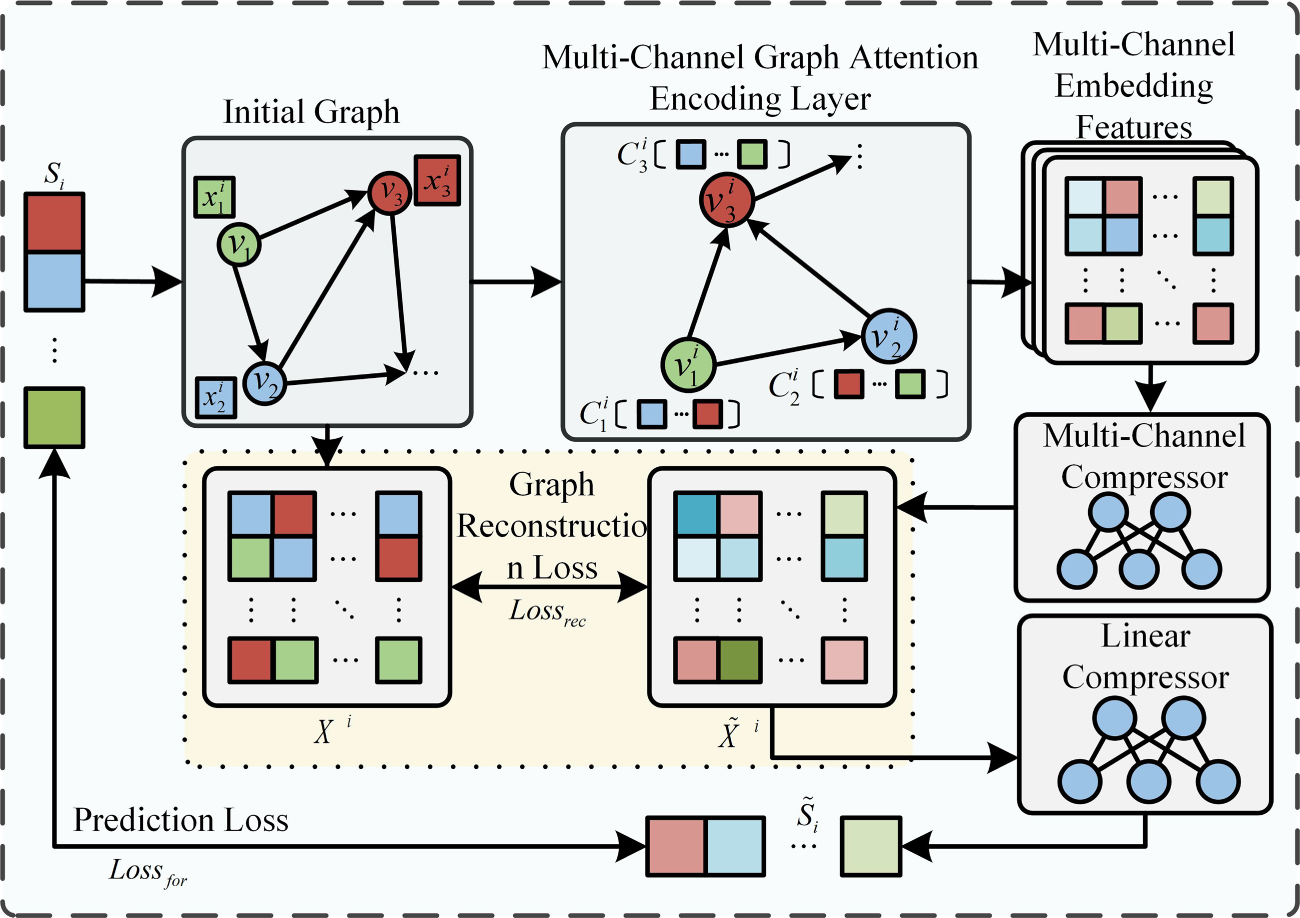
Figure 3: Optimization of graph structure learning

The primary objective of MC-GAL is to extract structural features among multiple variables from the initial graph and to aggregate their relational features. This is achieved for each node using a graph attention layer, as shown below.

ecj′i=τ(α→T⋅[wxc∥wxj])(6)

τ(x)=max(0,x)(7)

In the Eqs. (6) and (7), ecj′i denotes the updated edge weight between nodes vci and vji, ′||′ represents the concatenation operation, τ(⋅) is the activation function, α→T refers to the attention coefficient between nodes vci and vji, wvc and wvj represent linear transformations applied to nodes vci and vji to enhance their feature representation capability. Eq. (7) defines the computation of the activation function τ(⋅).

α→T=ecj′i∑k∈Ncieck′i(8)

The attention coefficient α→T is formulated in Eq. (8). Nci denotes the set of neighbors of vertex vci, which is obtained from the adjacency matrix Ai. Eq. (9) represents the updated embedding features of node vci.

xc′i=σ(∑k∈Ncieck′i⋅w⋅xk)(9)

To enhance the stability of the multi-channel graph encoding layer, a multi-head attention mechanism is introduced and integrated into the graph attention layer, resulting in the multi-channel graph attention layer. The computation of this layer is defined in Eq. (10), where H denotes number of channels. The outputs from different channels are fused via a concatenation operation, thereby enriching the node feature representations.

xc′i=‖h=1Hσ(∑k∈Ncieck′i⋅w⋅xk)(10)

In this study, the number of channels H is set to 3. In MC-GAL, each channel independently performs a self-attention computation to model structural dependencies between nodes from different subspaces. Increasing the number of channels enhances feature decomposition capability, but it also causes the parameter size and computational cost to grow linearly with H. Therefore, a balance between model expressiveness and computational efficiency is required. Considering the commonly used 3–4 channel configuration in multi-head attention mechanisms, this study ultimately adopts H=3 as the default setting to achieve feature encoding that balances expressive power and computational controllability.

(2)   Compressor:

The schematic diagrams of the multi-channel and linear feature compression modules are shown in Fig. 4. The multi-channel compression module is responsible for compressing features across multiple channels, while the linear compression module performs feature compression within a single channel. The detailed processes are described as follows.

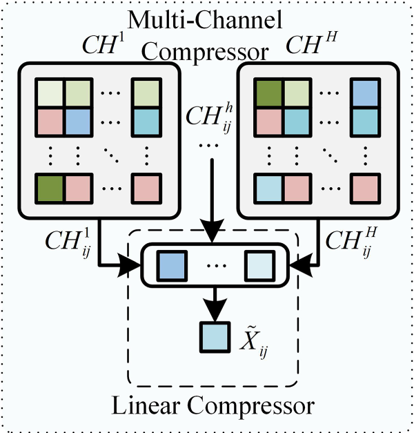
Figure 4: Multi-channel compressor and linear compressor

The multi-channel compression module is designed to facilitate the reconstruction Lossrec calculation between the optimized node features X′i∈RW×H×(M/H) from Gi and their initial embeddings Xi∈RW×M. This is achieved by applying a multi-channel compression function ε(X′i):RW×H×(M/H)↦RW×M, as shown in Eq. (11).

X~ji=τ([CHi,j1,⋯,CHi,jH]WH+BH)(11)

In this formula, WH and BH represent the weight matrix and the error matrix, respectively, while CHi,jh denotes the weight value at the i-th and j-th position in the h-th channel of X′i.

The linear compressor is designed to facilitate the calculation of the predicted loss Lossfor between X~i and the input Si, which is compressed using the linear compression function δ(X~i):RW×M↦RM, as shown in Eq. (12). Here, WS, BS represent the weight matrix and the error matrix, respectively.

S~i=δ(X~i)=X~WS+BS(12)

3.5 Node Feature Enhancements

To further enhance the representation of important features, this paper employs a single-channel attention mechanism, as illustrated in Fig. 5. The use of the single-channel attention mechanism allows GSL-AD to focus on variables with significant impact.

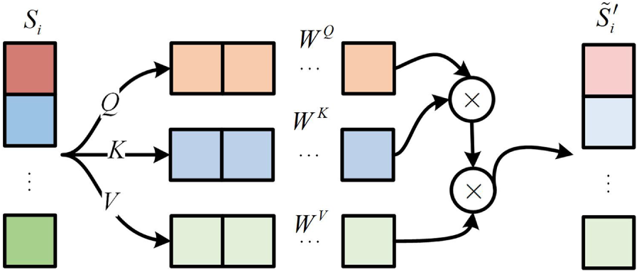
Figure 5: Single-channel self-attention mechanism

In this figure, the single-channel self-attention mechanism applies linear transformations to the input variable Si using the query weight matrix WQ, key weight matrix WK and value weight matrix WV, thereby enhancing the representation capacity for multivariate data. Eq. (13) defines the self-attention mechanism, whose output is S~i′, where d denotes the scaling factor for the weight vectors with d=M. Eq. (14) describes the fusion process of MC-GAL and the single-channel attention mechanism, where WF and BF represent the weight matrix and the error matrix, respectively.

S~i′=SoftMax{[SiWQ(SiWK)T]d}SiWV(13)

Zi=τ[(S~i∥S~i′)WF+BF](14)

3.6 Loss Function

To detect anomalies in multivariate data and explain the causes of variable anomalies within a graph-structured learning framework, this paper combines multi-channel graph encoding layers with a single-channel self-attention mechanism to extract and integrate multivariate data features and multivariate graph structure features, thereby improving anomaly detection accuracy and interpretability. The GSL-AD loss function is calculated as follows.

Eq. (15) represents the reconstruction error between the input data and the reconstructed data. Eq. (16) represents the prediction error between the input data and the predicted data. Eq. (17) defines the loss function of the GSL-AD model, which jointly considers both reconstruction and prediction errors to enhance anomaly detection performance, where α is a smoothing factor. Reconstruction error and prediction error exhibit distinct numerical characteristics: prediction error is more sensitive to local temporal perturbations and shows larger fluctuations, whereas reconstruction error is generally smoother but has limited ability to distinguish certain fine-grained anomalies. To prevent gradient instability caused by fluctuations in prediction error during training while maintaining responsiveness to anomalous changes, it is necessary to appropriately balance the weights between the two types of errors. Based on the commonly used range (0.8–0.9) in existing joint optimization frameworks and considering validation performance during the model development phase, this study sets the smoothing factor α to 0.85, ensuring a reasonable balance between training stability and sensitivity to anomalous changes.

Lossrec=∑i=1M∑c=1M(Xcji−X~cji)2(15)

Lossfor=∑j=1M(Sj−Zji)2(16)

Loss=αLossrec+(1−α)Lossfor(17)

3.7 Anomaly Score Calculation

The anomaly score in GSL-AD is obtained by weighting the prediction and reconstruction values. Prediction error is generally more sensitive to local temporal perturbations, whereas reconstruction error is numerically smoother but has weaker discriminative ability for structural shifts. Due to the differences in statistical scale and variation patterns between the two errors, a direct unweighted combination may allow prediction error to dominate in some scenarios, thereby amplifying noise. Introducing a hyperparameter enables effective balancing between the two, improving overall anomaly detection performance. The anomaly score is computed as follows:

prec=σ(Lossrec);vfor=σ(Lossfor)(18)

score=vfor+ς×prec1+ς(19)

To enhance model stability, the reconstruction and prediction losses are normalized using Eq. (18), where σ denotes the Sigmoid function. Eq. (19) defines the computation of the anomaly score. Based on the analysis of the distribution characteristics of the two types of errors, this study sets the hyperparameter ς to 0.35 to moderately suppress fluctuations in prediction error while retaining its sensitivity to temporally dependent anomalies, thereby achieving a more stable and discriminative anomaly score.

3.8 Anomaly Detection Algorithms

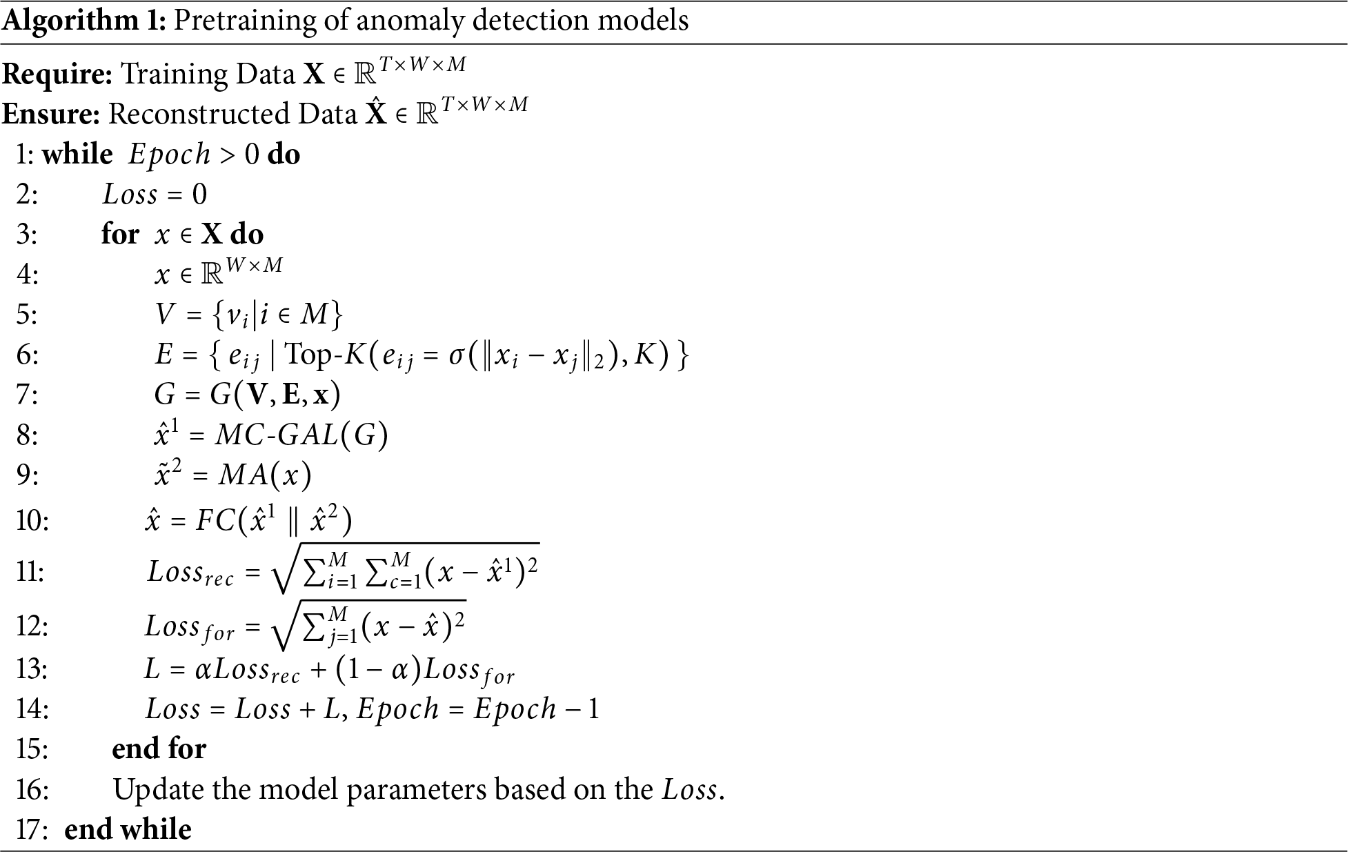
In this section, we provide a detailed description of the algorithm used to train the anomaly detection model.

In Algorithm 1, the input data is denoted as X∈RT×W×M, where T represents the number of sampled data segments, W is the sampling window length and M denotes the number of variables. Step 2 initializes the model loss. Steps 4–7 construct a multivariate coupling network based on a recommendation strategy to capture dependencies among variables. In Step 8, the edge weights of the coupling network are dynamically optimized. Step 9 enhances node representations through an attention mechanism to highlight important features. Steps 10–14 perform the fusion of structural and representational features, followed by the computation of prediction and reconstruction losses. Finally, in Step 16, the model is optimized using backpropagation based on the calculated loss.

In this paper, we perform anomaly detection on the test dataset using a pre-trained model. Anomalies are identified based on the reconstruction error and a dynamic threshold selection method is adopted to improve detection accuracy, as presented in Algorithm 2.

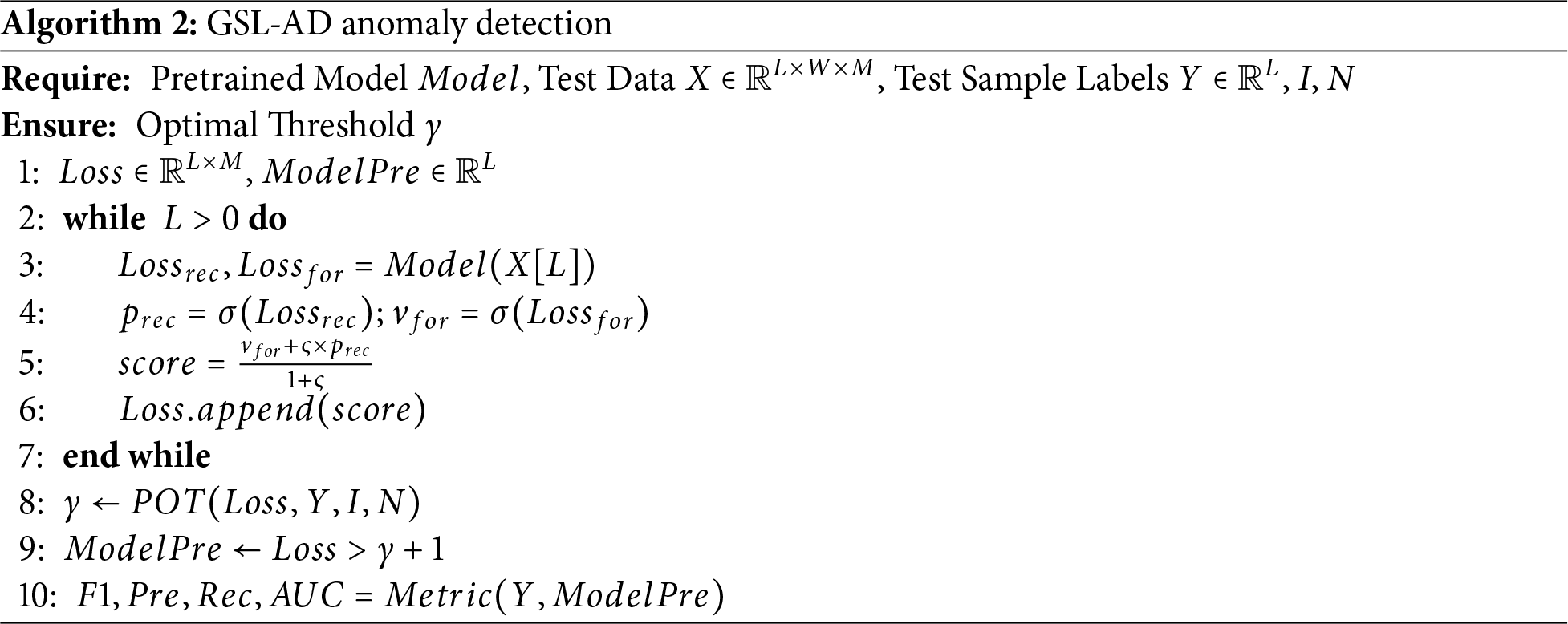
In Algorithm 2, the input is a pre-trained model and the test dataset X∈RL×W×M, where L denotes the number of sampled test segments, W is the sampling window length, M represents the number of variables, I and N are parameters for dynamic threshold selection. Steps 3–6 compute the reconstruction error of the test dataset using the pretrained model, with the results stored in Loss. In Step 7, the Peak Over Threshold (POT) method is employed to dynamically select the optimal threshold γ. Step 8 produces the model’s prediction results by comparing each element in Loss with γ: elements greater than γ are replaced with 1, and those less than or equal to γ are replaced with 0. Finally, Step 9 calculates the model’s evaluation metrics, including F1-score, Precision, Recall and AUC.

4  Experiments and Analysis

4.1 Datasets

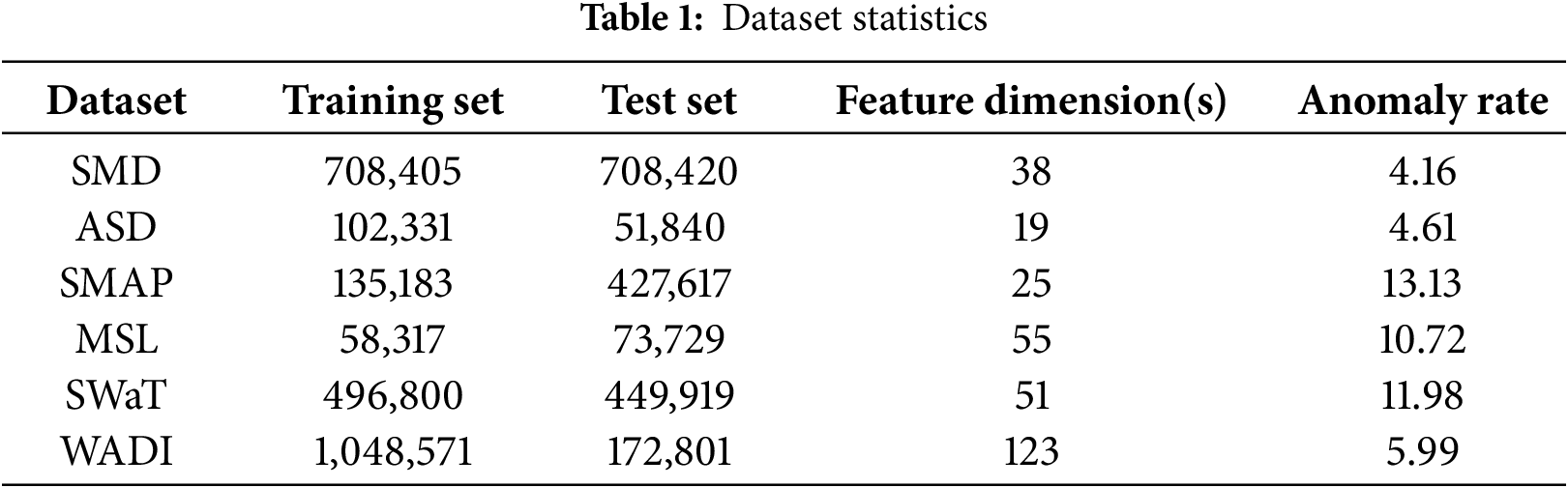
The datasets used in the experiments are listed in Table 1, including the Server Machine Dataset (SMD) and the Anomaly Simulation Dataset (ASD) [24], the Mars exploration mission datasets SMAP and MSL [25], and the water treatment system datasets SWaT and WADI [26,27]. Detailed descriptions are as follows.

•   SMD The server machine dataset (SMD) contains 5 weeks of stack trace monitoring data collected from a computer cluster. Due to changes in service modes during the data collection process, the training and test sets may follow different normal behavior patterns. To avoid the effects of distributional drift, we only select the subsets without such drift: Machine-1-1, Machine-2-1, Machine-3-2 and Machine-3-7.

•   ASD The application server dataset (ASD) monitors the operational status of application services running on servers. It contains data from 12 servers, where each instance describes the state of a specific server. The dataset spans 45 days of monitoring and includes 19 features representing various system metrics, such as CPU-related measurements, memory usage, network activity and virtual machine statistics.

•   SMAP The soil moisture active passive (SMAP) dataset, provided by NASA, containing soil sample data and telemetry collected via a Mars exploration probe. It primarily consists of sensor readings used for remote soil moisture monitoring.

•   MSL Similar to SMAP, the mars science laboratory (MSL) dataset includes sensor and actuator data from the Mars rover itself. To avoid the effects of data drift, we select the stable subsets A4, C2 and T1, it is similar to the approach used for the SMD dataset.

•   SWaT The secure water treatment (SWaT) dataset comprises operational monitoring data from a real-world water treatment plant, including 7 days of normal operations and 4 days of attack scenarios. The dataset contains sensor data (e.g., water levels and flow rates) and actuator states (e.g., valves and pumps).

•   WADI The water distribution (WADI) dataset is an extended version of SWaT. It includes 14 days of normal operations and 2 days of attack scenarios, capturing a broader range of water distribution system behavior.

4.2 Experiment Settings

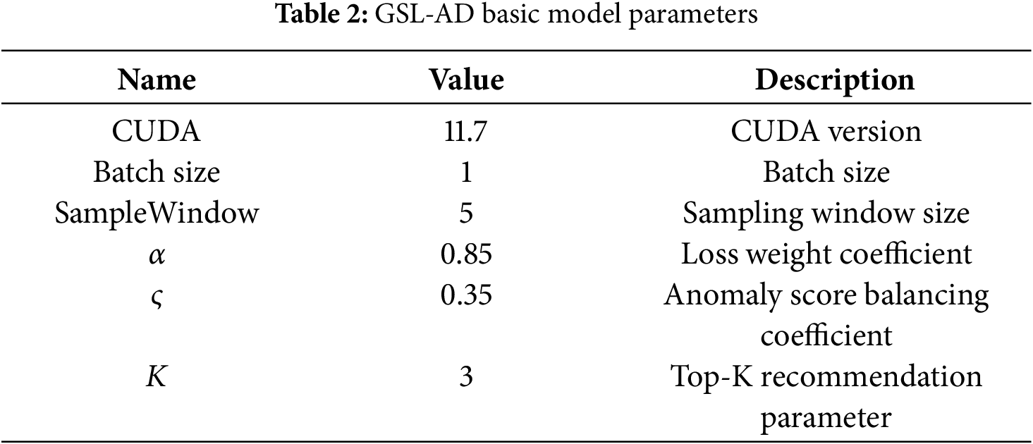
To evaluate the performance of GSL-AD on multivariate time-series anomaly detection tasks, we conduct a series of experiments, including comparative experiments, ablation studies, convergence stability analysis, hyperparameter analysis and visualization of anomaly causes. Additionally, we apply random permutation to the time steps of each dataset to investigate anomalies caused by temporal misalignment. The configuration details of the proposed model are summarized in Table 2.

4.3 Comparison Models

The following baseline models are selected for comparison in this study.

•   Models Based on Subsequence Matching MERLIN [28] is a method where anomalies are identified by measuring the similarity between incoming data and historical subsequences from the training data.

•   Models Based on Graph Neural Networks GDN [20] is an anomaly detection method that leverages graph neural networks to identify anomalies by comparing differences in graph structures. GAE [29] utilizes graph attention mechanisms to learn graph representations, which can be applied to anomaly detection tasks.

•   Reconstruction-Based Encoder-Decoder Models USAD [30] is an unsupervised anomaly detection method that identifies anomalies by reconstructing input data and measuring the reconstruction error. OmniAnomaly [22] combines variational autoencoders with graph-based structures to model multivariate time-series data for anomaly detection. DAGMM [31] integrates Gaussian Mixture Models with deep neural networks to learn latent representations of the data and detect anomalies based on reconstruction and compression errors.

•   Time-Series Forecasting Models MAD-GAN [32] is a method for multivariate anomaly detection that leverages Generative Adversarial Networks (GANs) to model temporal dependencies. LSTM-NDT [33] employs Long Short-Term Memory (LSTM) networks for sequence modeling and anomaly detection in time-series data. CAE_M [34] integrates Convolutional Autoencoders with a memory mechanism to capture complex temporal structures in multivariate time-series data and detect anomalies.

4.4 Results and Analysis

The evaluation metrics used in this study include Recall (Rec), Precision (Pre), Area Under the Curve (AUC), and F1-score (F1). The best results are highlighted in bold. If multiple methods achieve the same score for a given metric, no bolding is applied to indicate the absence of a unique best result.

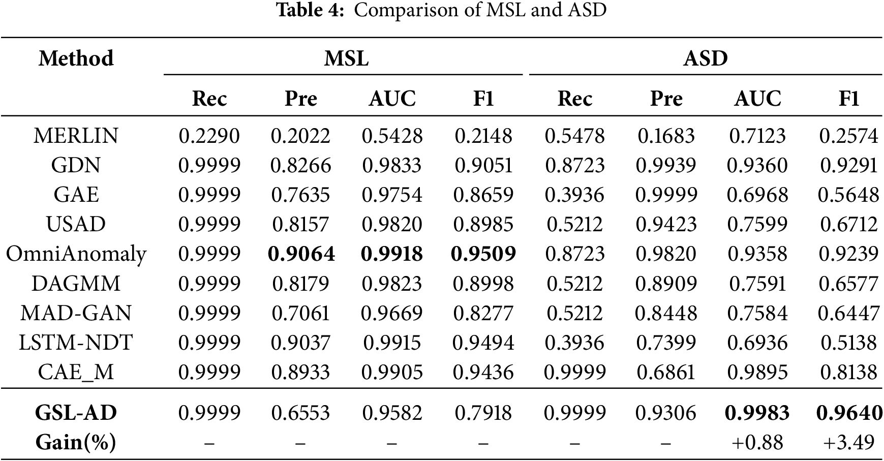
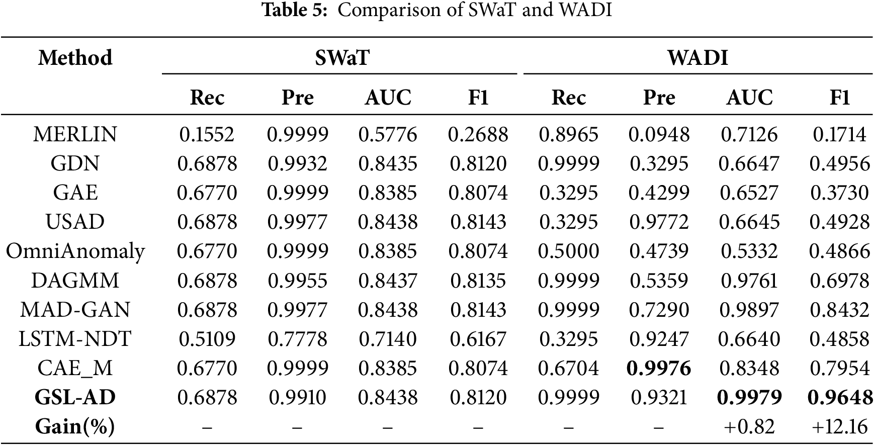
Table 3 presents the comparison results on the SMD and SMAP datasets, Table 4 shows the results for MSL and ASD and Table 5 summarizes the results for SWaT and WADI.

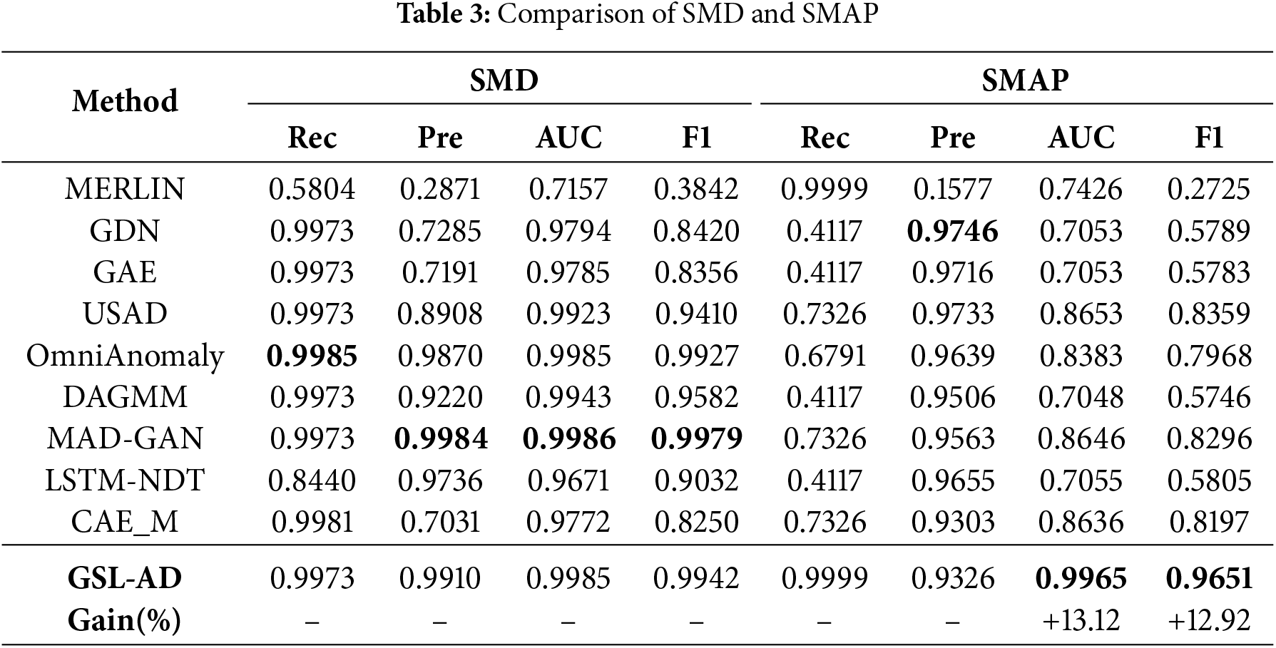
As shown in Table 3, both OmniAnomaly and MAD-GAN achieve relatively higher AUC scores on the SMD dataset but perform poorly on the SMAP dataset. This suggests that time-series reconstruction-based strategies may be limited in capturing low-dimensional feature relationships. In contrast, the proposed model explicitly models multivariate dependencies through a multivariate coupling graph network, effectively mitigating the negative impact of high-dimensional data on anomaly detection performance. It achieves superior results in both AUC and F1-score on the SMD and SMAP datasets, demonstrating strong generalization ability. These results indicate that incorporating graph structural features contributes effectively to improving anomaly detection performance.

As shown in Table 4, both OmniAnomaly and LSTM-NDT achieve superior performance in terms of AUC and F1-score on the MSL dataset, indicating that temporal features play a significant role in datasets with strong temporal dependencies. GDN shows the best F1 performance on the ASD dataset, further validating the effectiveness of graph-based structural learning in anomaly detection. Additionally, CAE_M achieves the highest AUC on ASD, suggesting that using convolutional encoders to compress time-series data helps to mitigate delayed causal effects in anomaly patterns. The proposed model outperforms others on the ASD dataset about both F1 and AUC, benefiting from the integration of multi-level, multi-channel features with multivariate structural information.

As shown in Table 5, GDN performs poorly in terms of Precision on the high-dimensional WADI dataset, indicating its limitations in embedding graph structural features under high-dimensional conditions. In contrast, the proposed model achieves superior AUC and F1-score on both the SWaT and WADI datasets, demonstrating that the graph-structure learning strategy plays a significant role in enhancing anomaly detection performance.

To comprehensively evaluate the overall performance of the proposed model, we compute the average values of all evaluation metrics for GSL-AD and the baseline models across different datasets, as shown in Fig. 6. It demonstrates that GSL-AD achieves the best overall performance in terms of average AUC, Recall, Precision and F1-score. The result suggests that the effective integration of complex inter-variable couplings and the multivariate coupling network topology through graph-structured reconstruction significantly reduces missed detections caused by temporal misalignments, thereby enhancing the robustness and adaptability of multivariate time-series anomaly detection models.

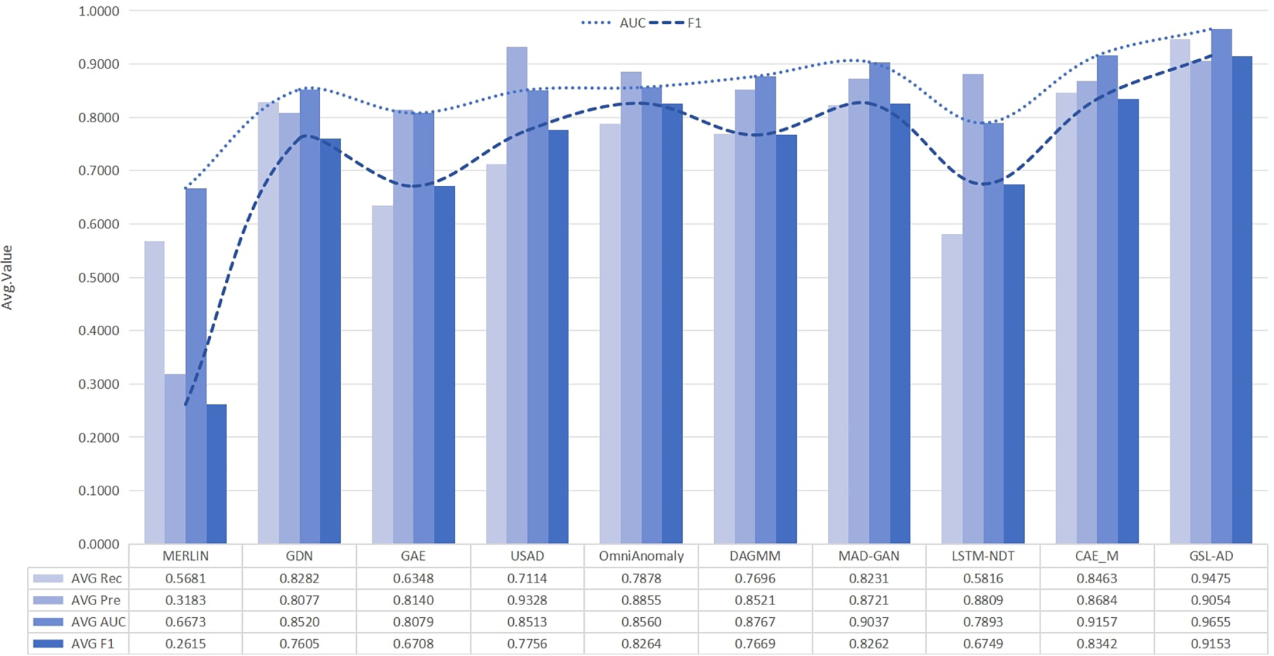
Figure 6: Comprehensive analysis of comparative experiments

4.5 Ablation Study

To further investigate the impact of the multi-channel graph attention encoding module, the multi-head attention mechanism, and different fusion strategies on the anomaly detection performance of the proposed model, we conduct ablation studies.

•   No-MA The multi-head attention module is removed, and feature fusion is performed via concatenation.

•   No-MC-GAL The multi-channel graph attention encoding module is removed, and feature fusion is performed via concatenation.

•   No-FC The fully connected layer is removed, and feature fusion is performed via concatenation.

•   No-POT The dynamic threshold selection module is removed, and feature fusion is performed via concatenation.

•   FM1 The corresponding outputs of MA and MCGAL are summed element-wise.

•   FM2 The corresponding outputs of MA and MCGAL are combined by element-wise multiplication.

•   FM3 The outputs of MA and MCGAL are combined via concatenation.

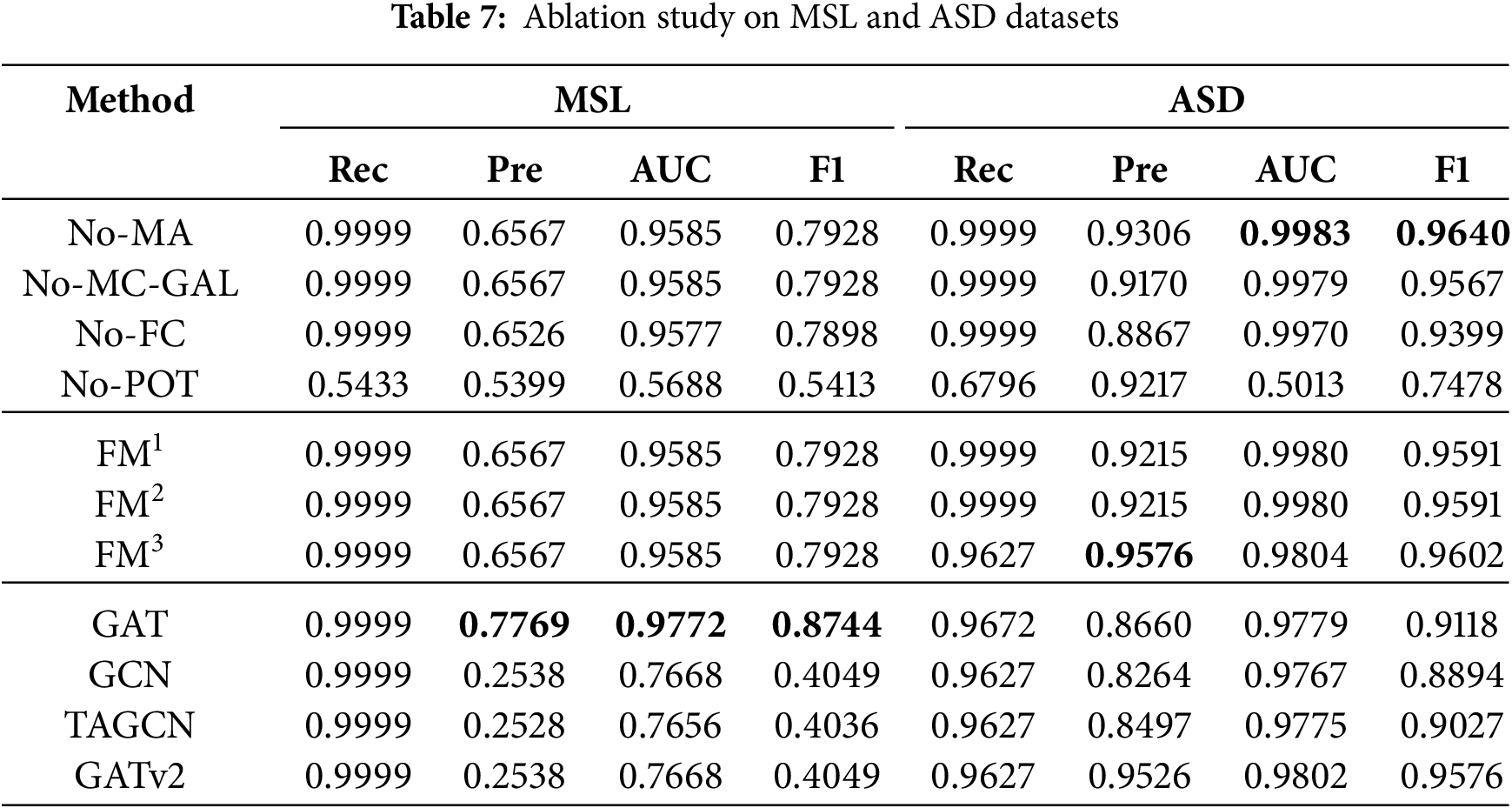
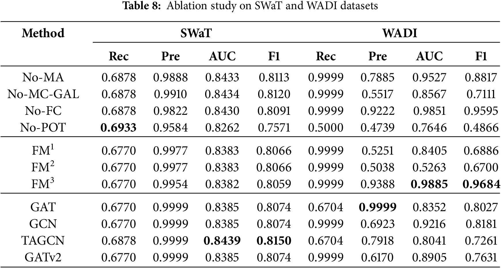
This study selects GAT, GCN, TAGCN and GATv2 as baseline models for comparison with GSL-AD. Table 6 shows the ablation experiment results on the SMD and SMAP datasets, Table 7 on the MSL and ASD datasets, and Table 8 on the SWaT and WADI datasets. The best results are highlighted in bold. If multiple values for an evaluation metric are the same, no bold formatting is applied, indicating the absence of a unique optimal result. Detailed analysis is as follows.

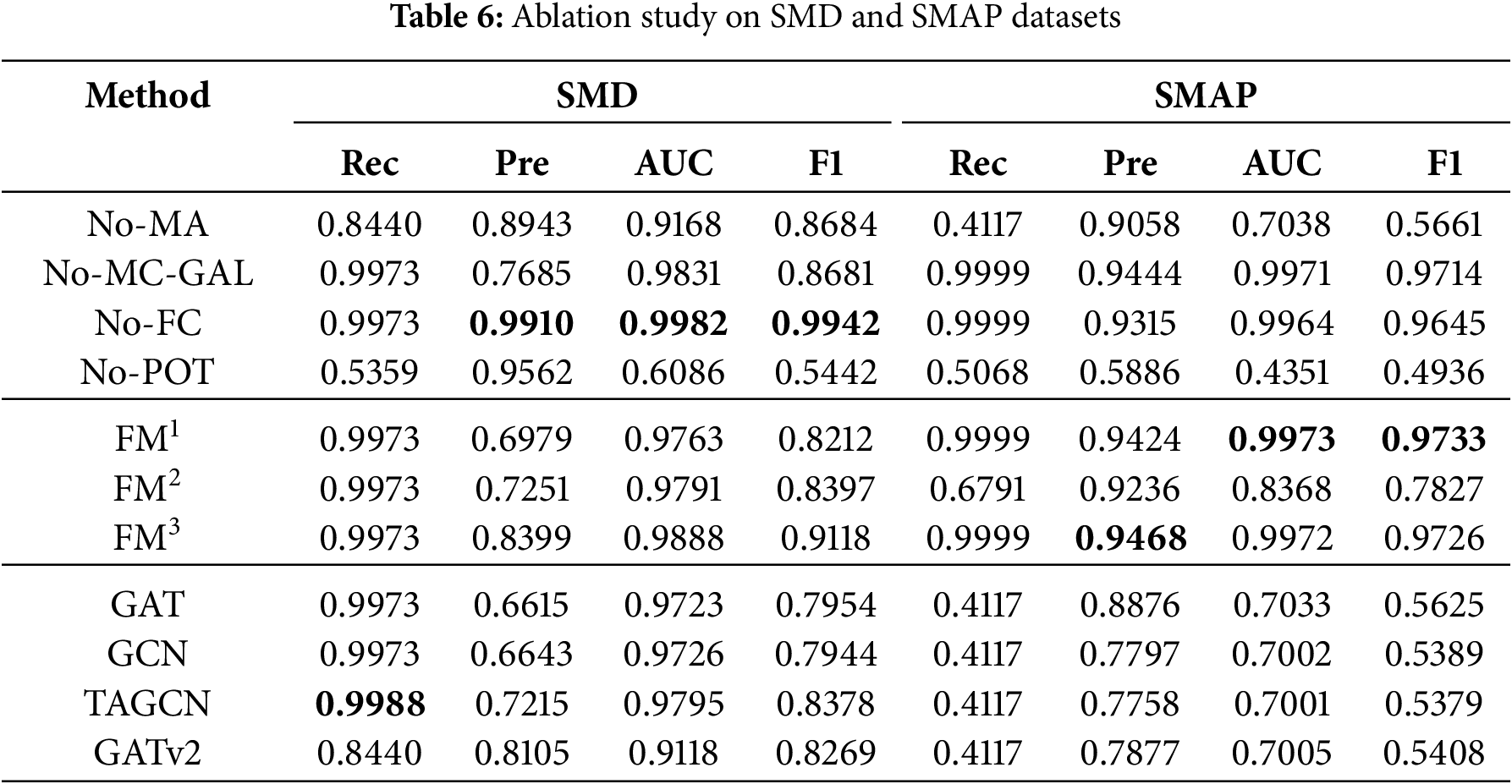
As shown in Table 6, feature concatenation outperforms element-wise addition and multiplication in terms of AUC and F1 on both the SMD and SMAP datasets, offering more stable and superior results. This indicates that concatenation better captures the diversity of feature representations, thereby enhancing anomaly detection performance.

As shown in Table 7, the models exhibit a clear structural pattern. Models such as GAT, No-MA, and No-MC-GAL achieve relatively high AUC and F1 scores on the MSL dataset. This suggests that the simplified model architectures can yield competitive anomaly detection performance for datasets with well-defined structural features.

As shown in Table 8, FM3 achieves the highest AUC and F1 scores on the WADI dataset, indicating that the proposed model effectively captures the structural features inherent in WADI.

In summary, from the perspective of the fusion between MC-GAL and MA, FM3 achieves the best performance across multiple datasets. Its advantage primarily arises from MA, which emphasizes capturing local dependencies and attention weights among multivariate variables, while MC-GAL focuses on global topological features based on the graph structure. The two exhibit clear complementarity in the representation space. Meanwhile, the concatenation strategy preserves both local and global features without prior information compression, allowing subsequent modules to adaptively select from a richer representation space, thereby yielding superior detection performance.

In addition, to facilitate a comprehensive comparison of anomaly detection methods, we average each evaluation metric across all datasets. The results are shown in Fig. 7. The No-FC variant achieves the best average AUC and F1 performance across different datasets. This demonstrates that optimizing the topology of the multivariate coupling network through MC-GAL, enhancing node representations via attention mechanisms, and effective fusing structural and representational features can significantly improve the model’s capacity for anomaly representation. Therefore, the No-FC variant is selected as the final architecture for GSL-AD.

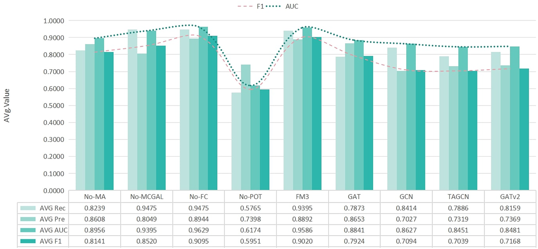
Figure 7: Comprehensive analysis of comparative experiments

4.6 Convergence Stability Analysis

To examine the stability of loss reduction in the model across various datasets, we analyze the trend of the loss function for epochs from 30 to 60. The results are presented in Fig. 8.

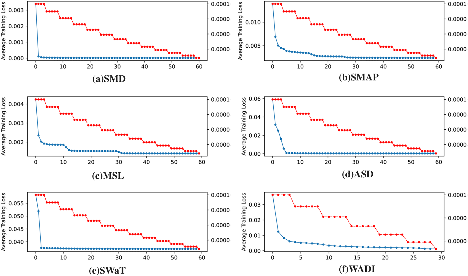
Figure 8: Loss curves of GSL-AD on different datasets

As shown in Fig. 8, both the training loss curves (in blue) and the testing loss curves (in red) of the GSL-AD model exhibit a consistently decreasing trend across different datasets, indicating that the model maintains stable performance under various data conditions.

4.7 Hyperparameter Analysis

To ensure consistency, “Time/s” on the vertical axis in the hyperparameter experiments indicates training time in seconds.

(1) The Sliding Window Length: To investigate the impact of different sliding window lengths on the detection performance of the proposed model, experiments are conducted with different window lengths such as 5, 10, 20, 40, 80, and 100. The results are illustrated in Fig. 9.

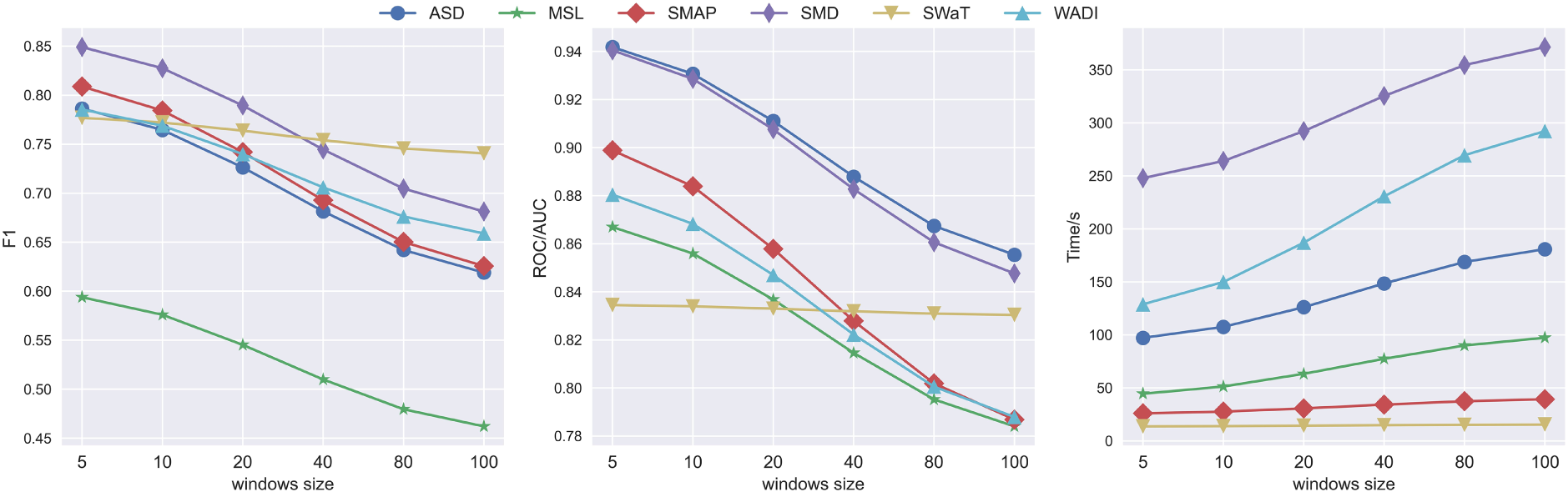
Figure 9: The impact of sliding window length on the anomaly detection performance of GSL-AD

Fig. 9 shows that as the sliding window length increases, the GSL-AD model exhibits a gradual decline in F1-score and AUC on the ASD, MSL, SMAP, SMD, and WADI datasets, while the training time increases. The best performance is observed when the window length is set to 5. This phenomenon can be attributed to the fact that anomalies in multivariate time-series data are often abrupt; longer temporal windows tend to smooth out local variations, thereby suppressing distinctive anomaly patterns and degrading detection accuracy. To further assess the impact of window size, the average evaluation metrics across all datasets are calculated, as illustrated in Fig. 10.

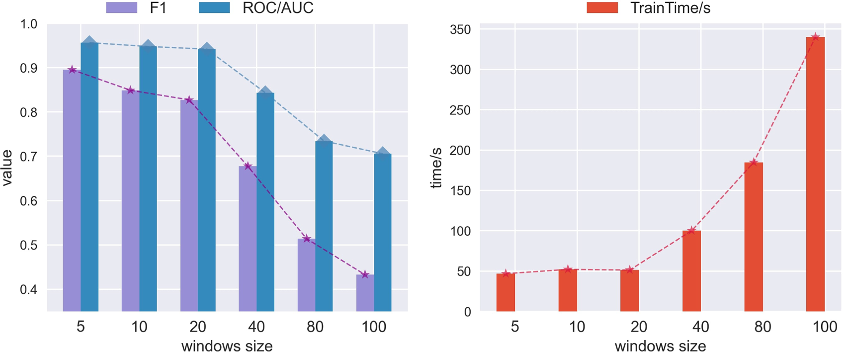
Figure 10: The impact of sliding window length on the overall anomaly detection performance of GSL-AD

Fig. 10 shows that the proposed model achieves its best performance and shortest runtime when the sliding window length is set to 5.

(2) MA Head: To investigate the impact of the number of MA heads on the detection performance of the proposed model, experiments were conducted with 1, 2, 4, 6 and 8 heads, respectively, as shown in Fig. 11.

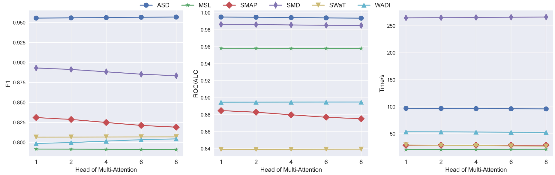
Figure 11: The impact of MA heads on the anomaly detection performance of GSL-AD

Fig. 11 shows that as the number of MA heads increases, the F1 score of the GSL-AD model gradually decreases on the SMD and SMAP datasets with a similar decline in AUC on the SMAP dataset. However, the F1 score on the WADI dataset increases. This indicates that the relationship between the number of multi-head attention channels and model performance improvement is nonlinear. To provide a comprehensive evaluation of MA heads influence on the proposed model, the average metrics across all datasets are shown in Fig. 12.

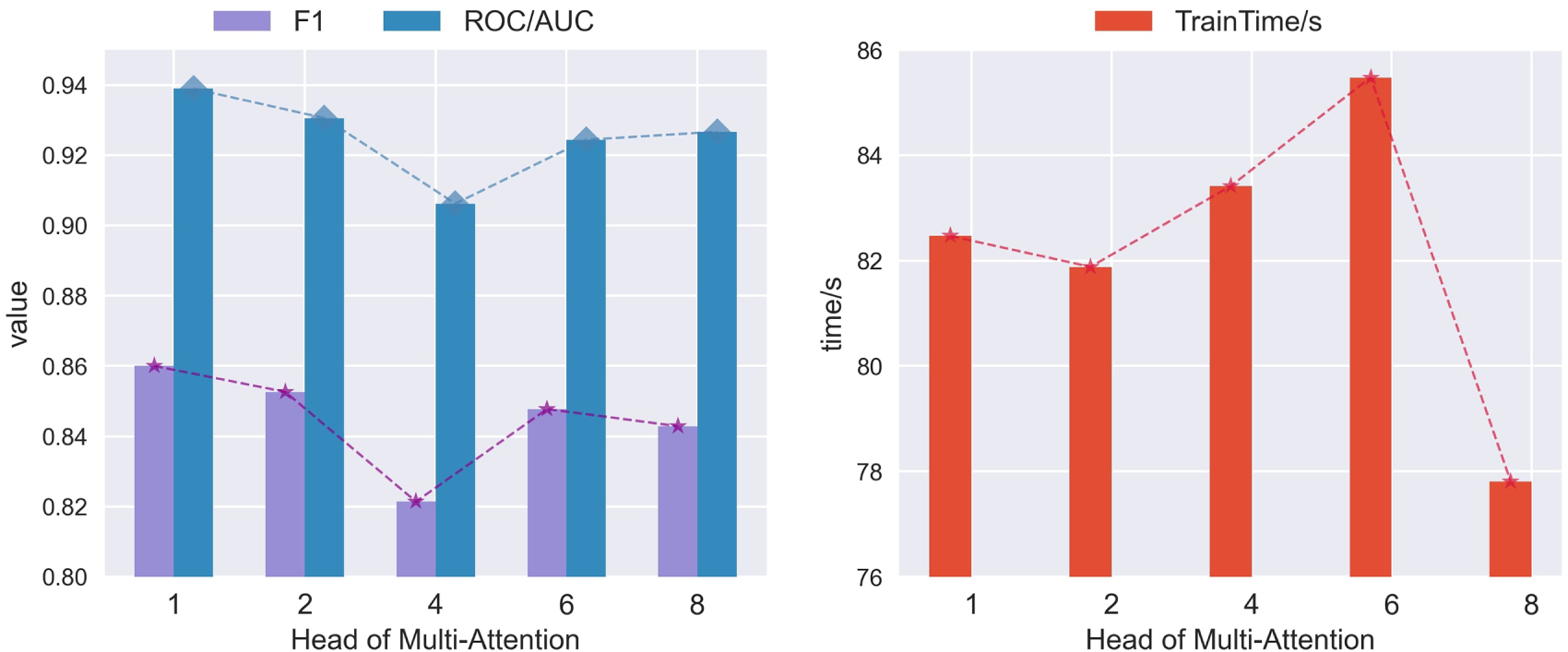
Figure 12: The impact of MA head on the comprehensive anomaly detection performance of GSL-AD

As shown in Fig. 12, the model achieves the best performance and reduced training time when the number of MA heads is set to 1.

(3) MC-GAL Head: To investigate the impact of the number of MC-GAL heads on the detection performance of the GSL-AD model, experiments are conducted with different head, which is set to 1, 2, 4, 6 and 8, as shown in Fig. 13.

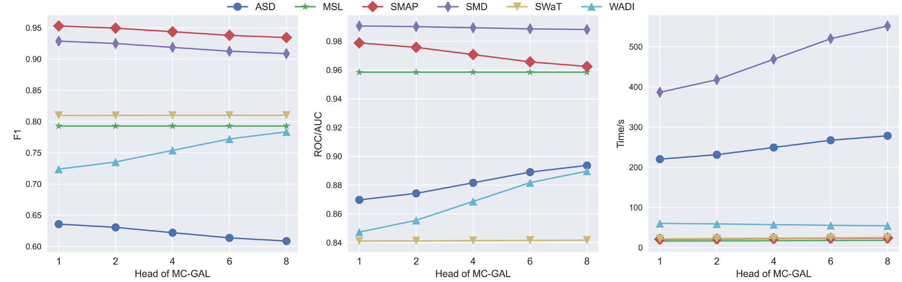
Figure 13: The impact of MC-GAL head count on the anomaly detection performance of GSL-AD

As shown in Fig. 13, increasing the number of MC-GAL heads leads to noticeable improvements in AUC on the ASD and WADI datasets. However, both F1 and AUC scores on the SMAP dataset gradually decline, and training time consistently increases. This suggests that simply stacking more attention heads in the multivariate coupling network does not necessarily enhance anomaly detection performance. To comprehensively assess the impact of the number of MC-GAL heads on model performance, we compute the average evaluation metrics across different datasets, as illustrated in Fig. 14.

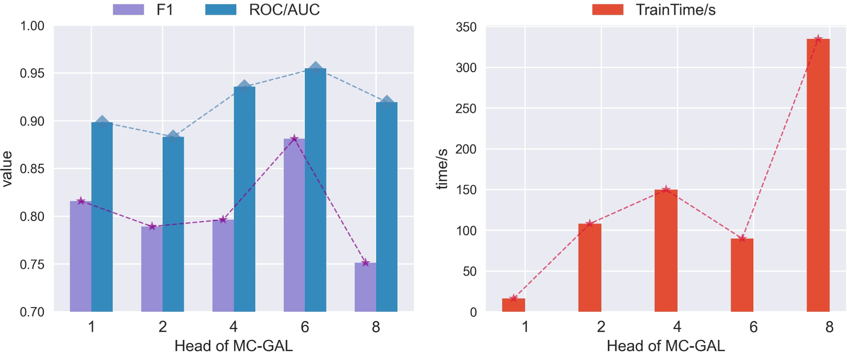
Figure 14: The impact of the number of MC-GAL heads on the overall anomaly detection performance of GSL-AD

As shown in Fig. 14, the model achieves the best performance and shorter training time when the number of MC-GAL heads is set to 6.

4.8 Visual Analysis of Anomalies

Anomaly visualization in multivariate time-series detection provides system operators with clear information on the timing and location of anomalies, facilitating efficient diagnosis and resolution. In this study, two primary methods are employed to analyze the causes of anomalies. First, the multivariate anomaly diagnosis method compares the true anomaly locations with those detected by the model, helping operators quickly identify the exact time and position of anomalies. Second, by visualizing the structural patterns of multivariate anomalies, the model clearly illustrates the graph topology of the multivariate coupling network. This enables operators to better understand the interactions among variables and perform a more comprehensive analysis of the underlying causes of anomalies.

Multivariate anomaly diagnosis aims to evaluate the performance of multivariate anomaly detection models. Firstly, abnormal points are labeled across different variables within the multivariate time-series data. Secondly, anomaly scores generated by the detection model are compared against a selected threshold. Finally, data points are classified as normal or abnormal based on this threshold, and the results are visualized with corresponding annotations. To facilitate understanding of the diagnostic process, a detailed explanation of the multivariate anomaly diagnosis legend is provided, as illustrated in Fig. 15.

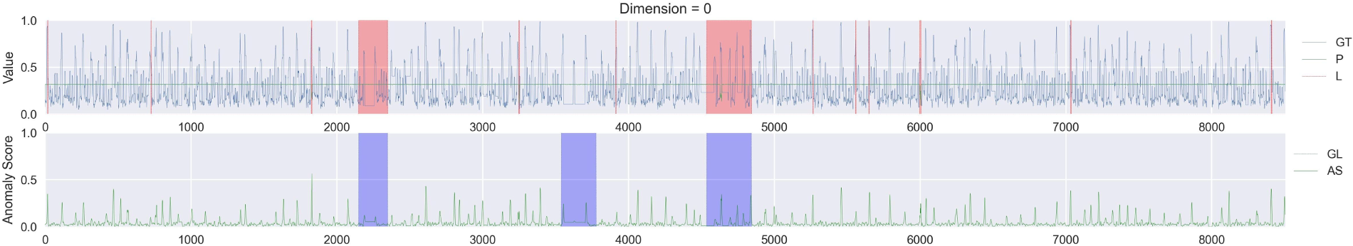
Figure 15: Explanation of the anomaly diagnosis legend

In Fig. 15, the upper part of the legend includes GT (the truth monitoring data), P (the predicted data), and L (the predicted anomalous data). The lower part includes GL (the true anomaly labels) and AS (the anomaly scores).

Multivariate anomaly structure visualization aims to reveal the structural changes between normal and anomalous states in multivariate data. This visualization module constructs multivariate coupling networks by taking normal data, anomalous data, and the reconstructed data generated by the anomaly detection model as input. To facilitate the interpretation of structural changes, the elements in the multivariate anomaly structure visualization are illustrated.

In Fig. 16, the left, center and right subfigures represent the graph structures of the normal data, the true anomalous data, and the reconstructed output from the anomaly detection model, respectively. Each node in the graph corresponds to a variable index in the multivariate anomaly detection dataset.

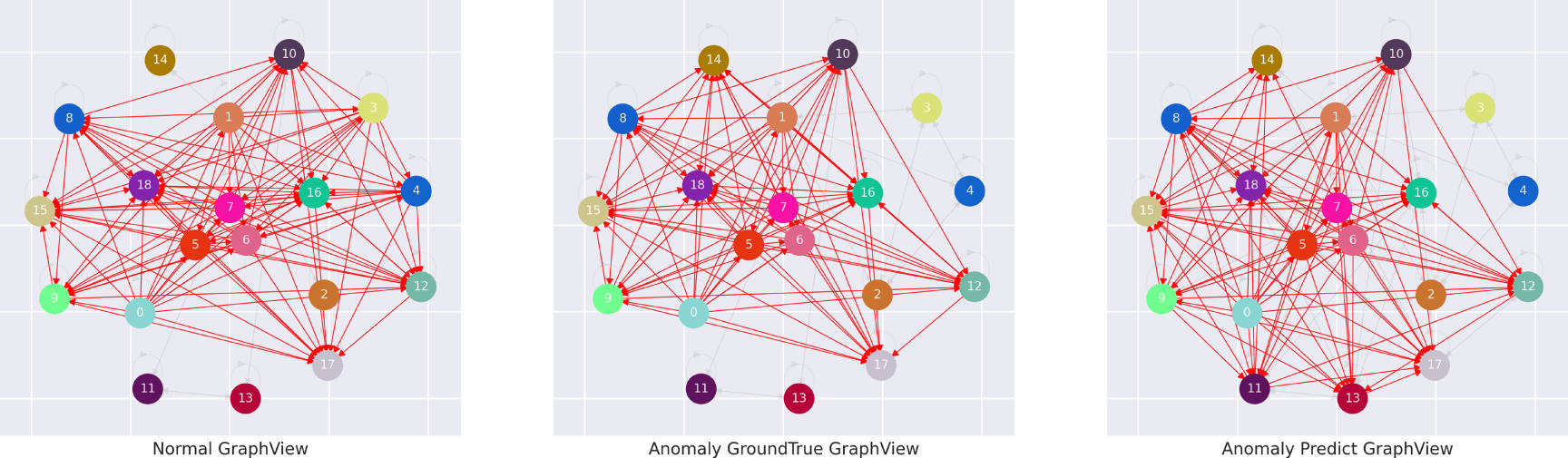
Figure 16: Legend description of anomalous structure elements

Tables 9–14 present the multivariate anomaly detection and diagnosis results of the proposed GSL-AD model, CAE_M and GAT on the SMD, SMAP, MSL, ASD, SWaT and WADI datasets, respectively.

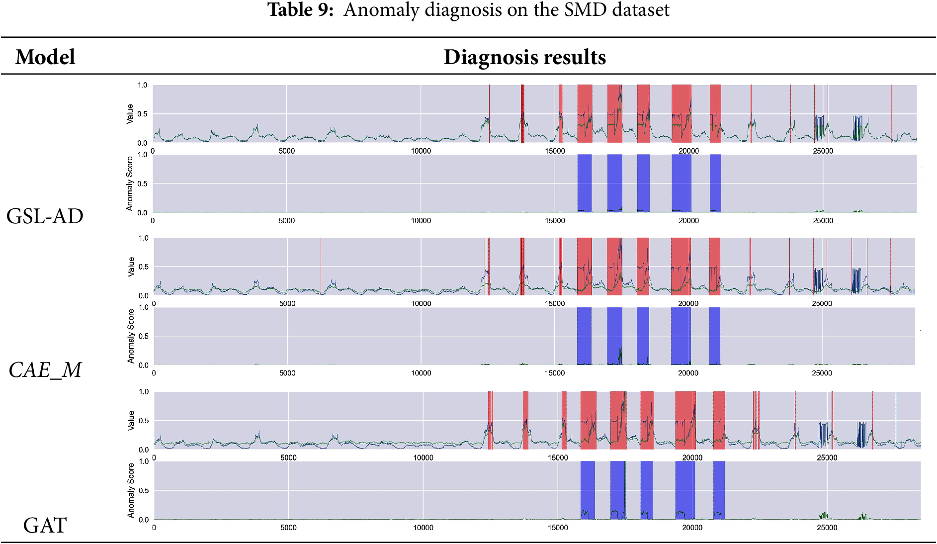
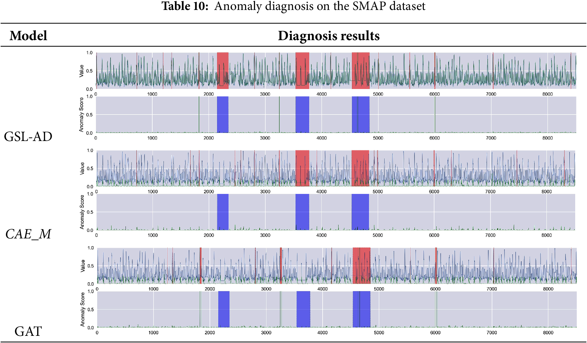
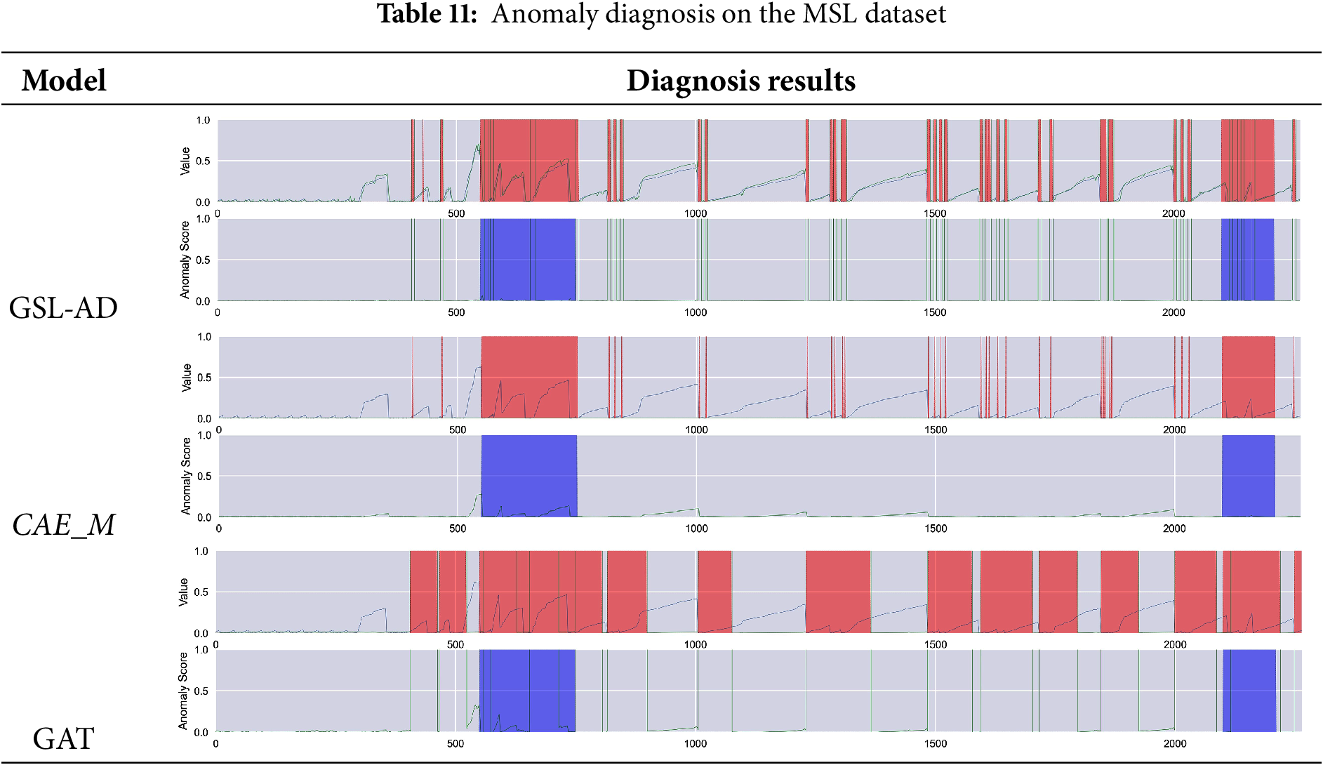
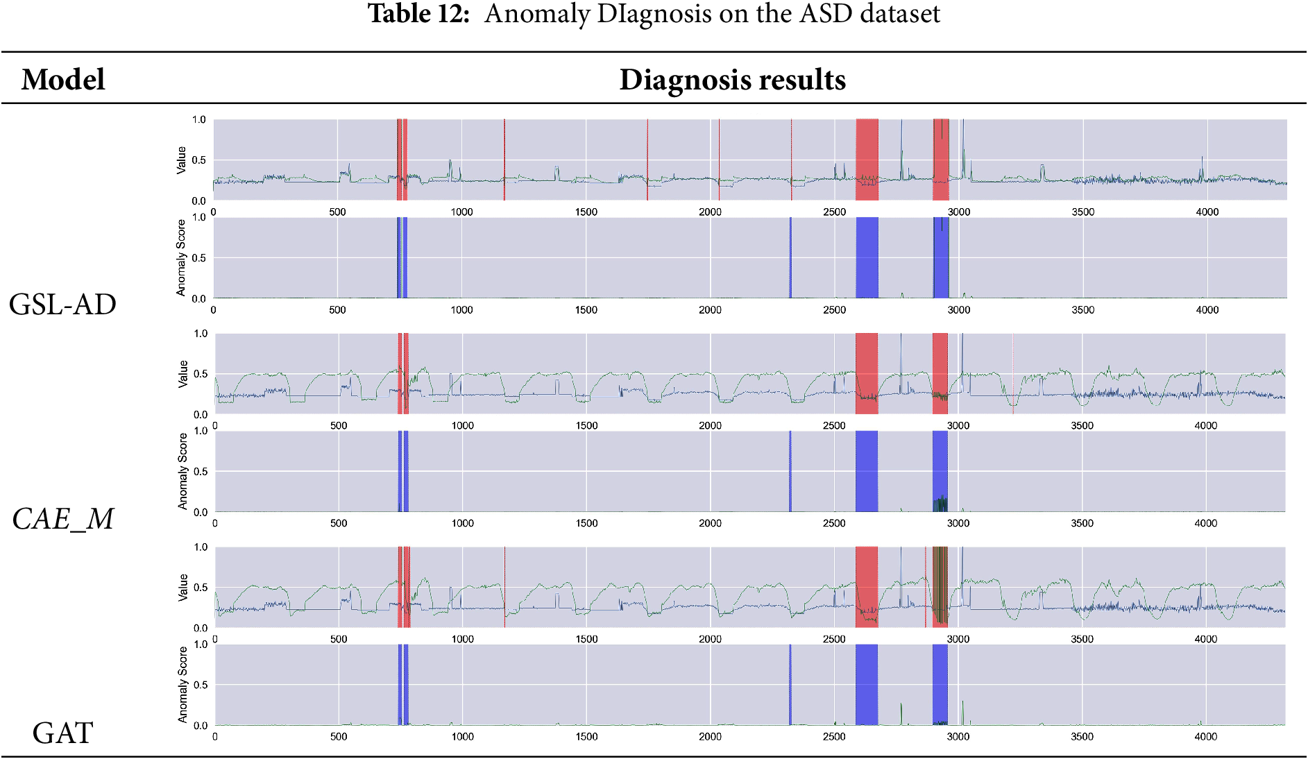
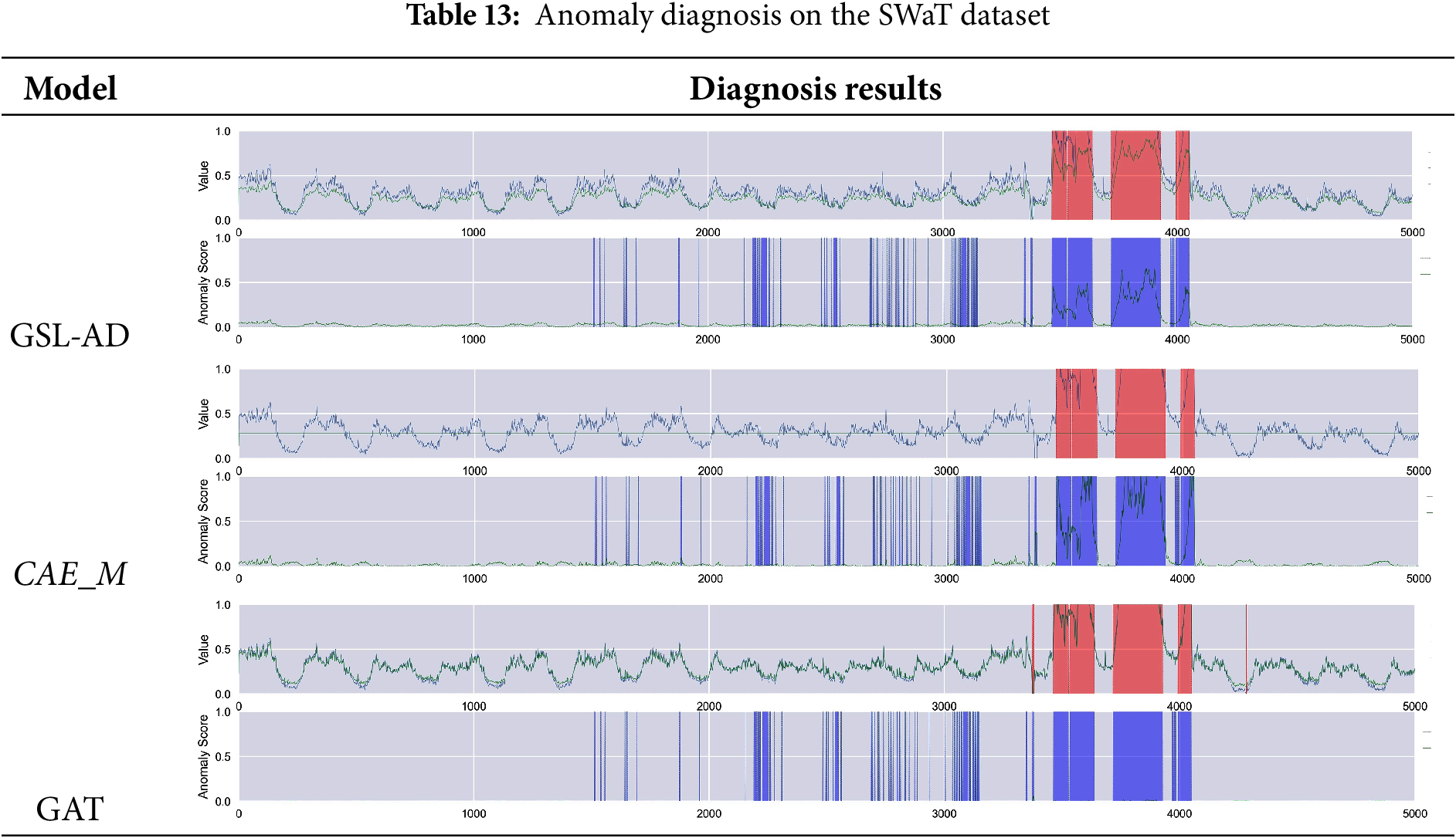
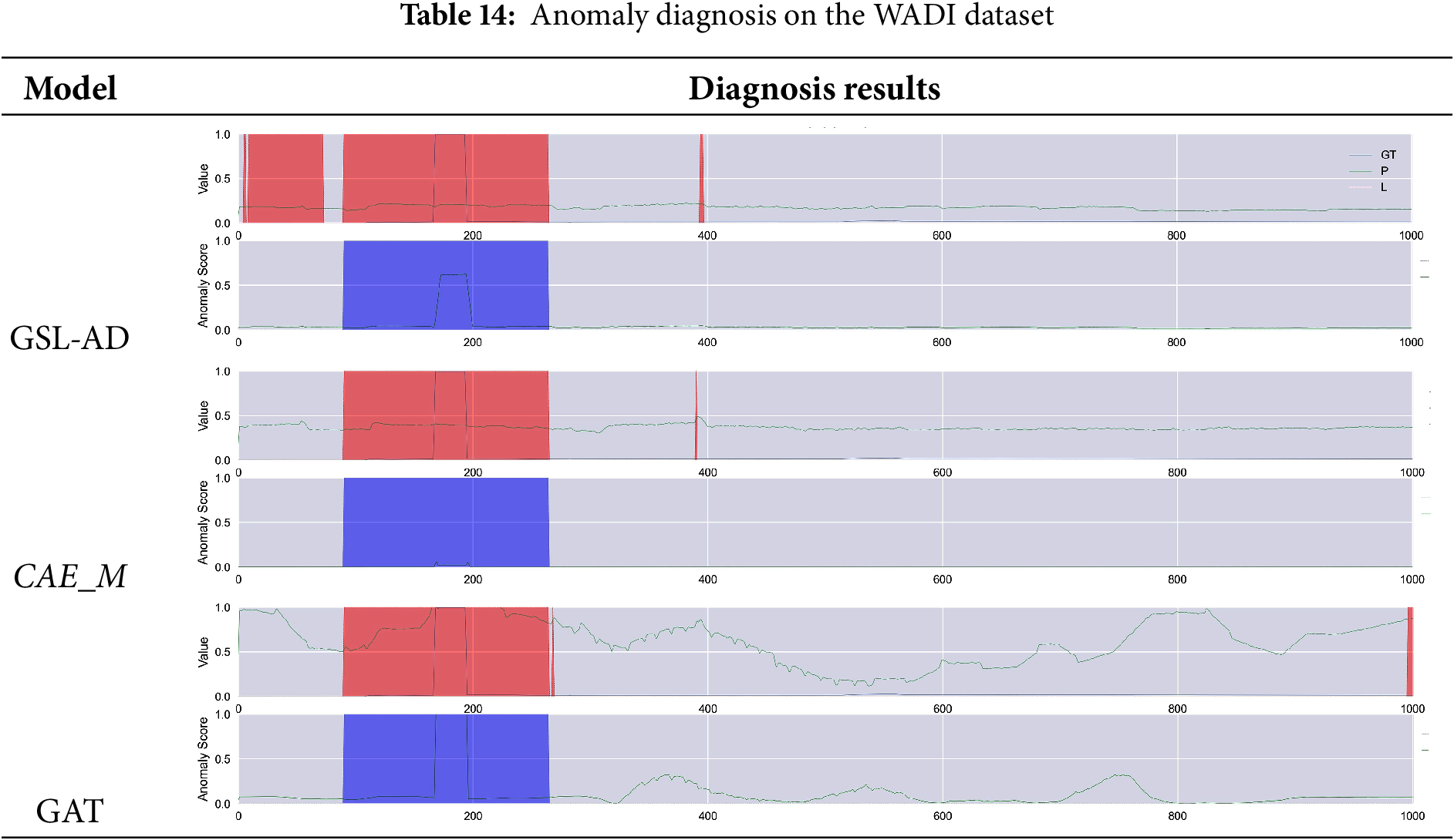
The diagnostic results of the GSL-AD model across different datasets demonstrate its ability to accurately identify anomalies in the SMD, SMAP, MSL, ASD, and WADI datasets. Compared to the CAE_M and GAT models, GSL-AD achieves a lower false positive rate and exhibits stronger robustness.

Tables 15–19 present the comparative results of multivariate anomaly structure analysis between the GSL-AD model and GAT on the SMD, SMAP, MSL, ASD and WADI datasets, respectively.

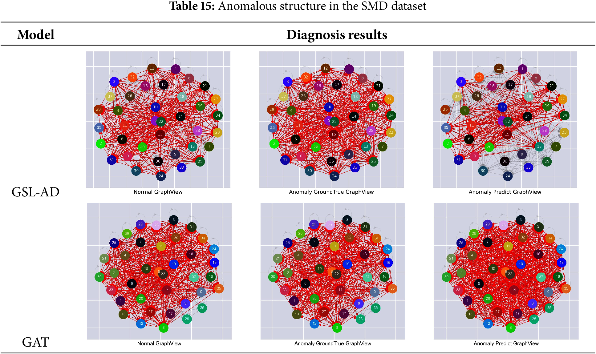
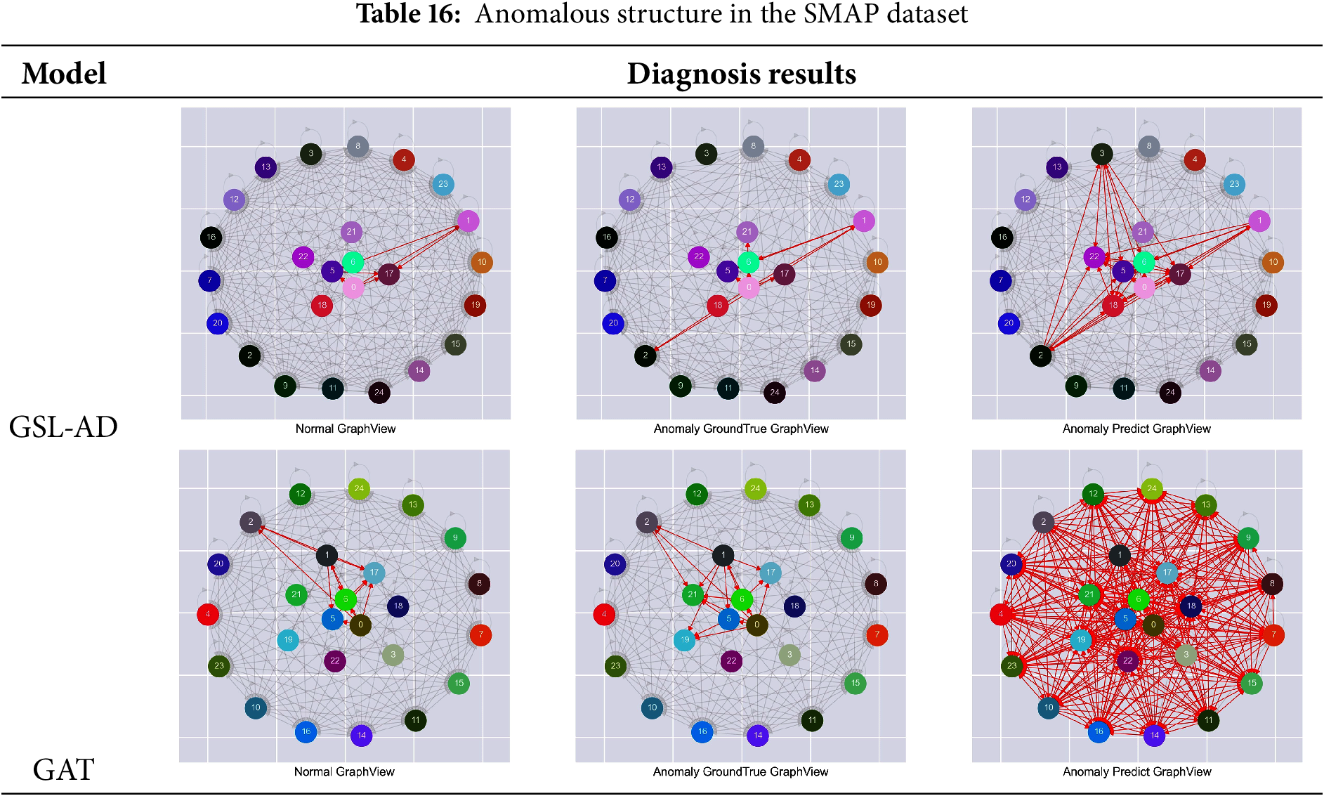
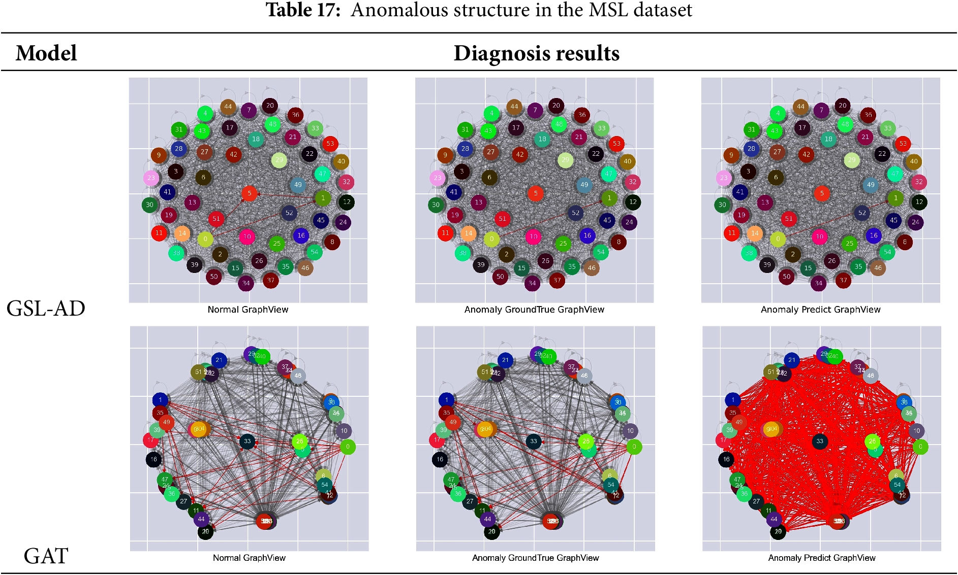
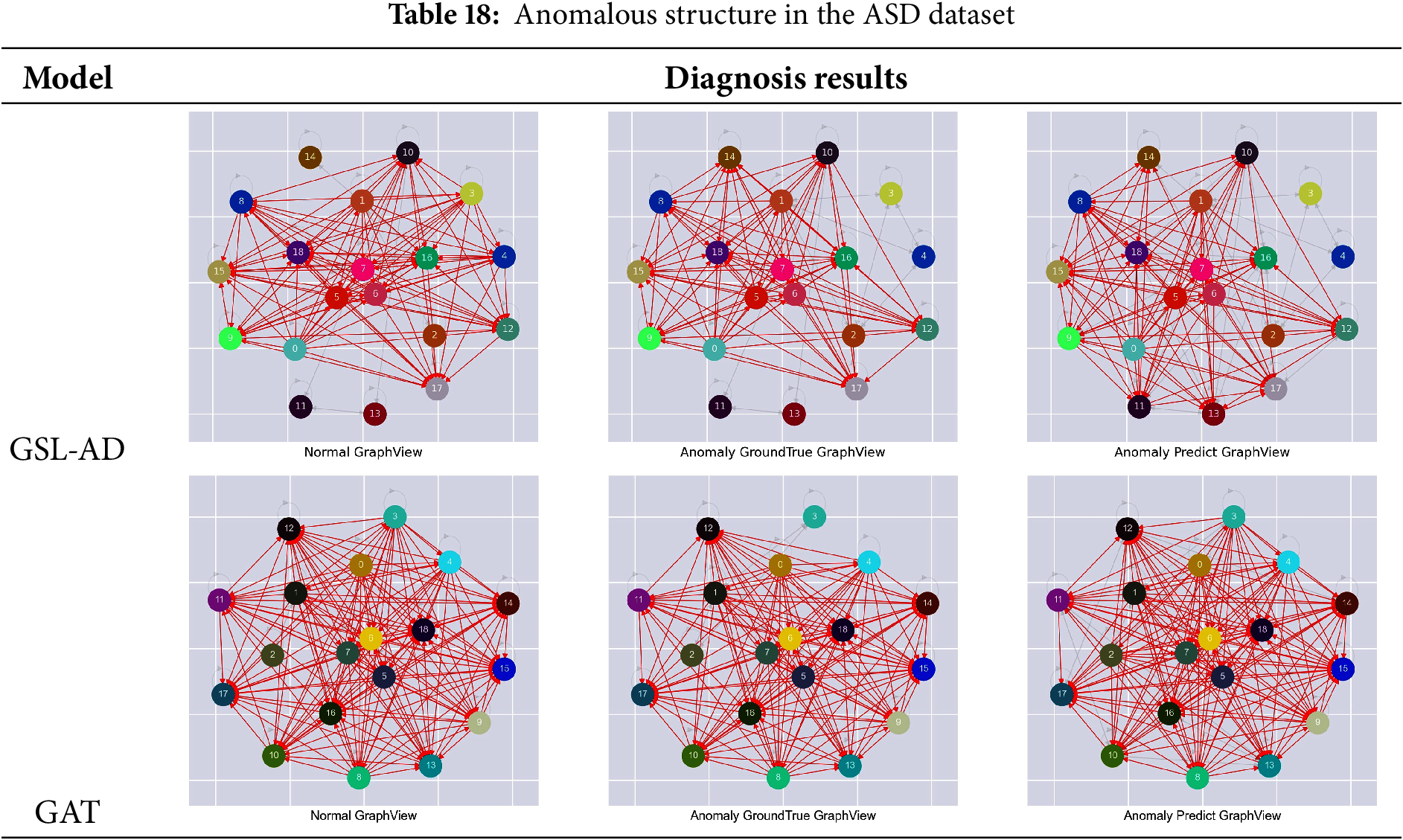
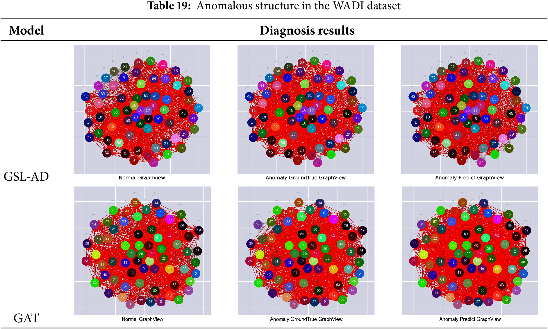
Table 15 shows that the anomaly detection results of the GSL-AD model contain a larger number of isolated nodes, while the isolated nodes in normal and anomalous data are relatively few. The GAT model detects fewer isolated nodes compared to GSL-AD, indicating that GSL-AD can effectively suppress variables with lower correlation.

Table 16 shows that the GSL-AD model detects a significantly higher number of correlated variables in anomalous data compared to the structures of normal and original anomalous data. The GAT model detects more correlated variables than GSL-AD, indicating that the proposed model effectively suppresses redundant multivariate correlations when constructing dense graph structures.

Table 17 shows that the variables associated with the GSL-AD model have significantly fewer associations compared to the structure of normal and abnormal data. The GAT model detects more associated variables than the GSL-AD model, indicating that the model in this paper is able to efficiently construct multivariate association features in terms of sparsity in constructing graph structures.

Table 18 shows that the anomaly detection results of the GSL-AD model exhibit a noticeable increase in isolated nodes compared to the graph structure of normal data. In contrast, the graph structure detected by the GAT model is more similar to that of the normal data, but shows significant differences from the actual anomalous graph structure. This suggests that the graph structure of anomalous data may manifest either as an increase or a decrease in isolated nodes.

Table 19 shows that the number of isolated nodes in the anomaly detection results of the GSL-AD model is significantly reduced compared to the graph structure of the actual anomalous data. In contrast, the detection results of the GAT model are more similar to the graph structure of normal data. However, they exhibit a noticeable increase in isolated nodes relative to the true anomalous structure. This indicates that isolated nodes may still persist even as data density increases on high-dimensional datasets like WADI.

The visualization results of anomaly structures across different datasets indicate that changes in isolated nodes, inter-node connections, and the sparsity or density of the graph structure can all disrupt the intrinsic relationships among variables, thereby leading to anomalies. These findings further highlight the significance and complexity of multivariate anomaly data structures in anomaly detection, offering valuable insights for future research.

5  Conclusion

To address the anomaly detection challenges caused by misaligned temporal dependencies in multivariate time series data, this study investigates the complex coupling relationships among variables and the effectiveness of integrating multivariate coupling network topologies under graph structure learning. By enhancing the spatial structural representation of multivariate data and reducing dependence on historical prior information, we propose a novel multivariate anomaly detection model based on graph structure learning.

Firstly, a Top-K recommendation algorithm is used to construct a sequence of candidate node relationships. The strength of coupling between nodes is measured using the narrow Minkowski distance and these relationships are ranked in descending order. By adjusting the value of K, the desired level of sparsity can be selected, enabling the construction of a multivariate coupling network topology. Secondly, we design a multi-channel graph encoding layer and a multi-stage channel compressor to efficiently extract, refine, and reconstruct the topological features of the multivariate coupling network. Furthermore, we introduce a single-channel attention mechanism to enhance the representation of multivariate data features and effectively integrate structural information, thereby improving the model’s representation capability. Finally, we enhance the model’s stability by computing a weighted combination of the structural reconstruction loss and the predictive loss of representation features to generate the anomaly score. This score is then used as the input to the unsupervised anomaly detection method POT with a dynamically selected threshold. This study adopts a two-stage training strategy, consisting of pre-training and fine-tuning phases, to further enhance the adaptability of the anomaly detection model. Experimental results demonstrate that the GSL-AD model achieves average AUC, Recall, Precision, and F1 scores of 96.55%, 94.75%, 90.54%, and 91.53%, respectively, across several datasets, outperforming existing methods. These findings further validate the effective integration of multivariate coupling network structures and learned feature representations, which successfully mitigate anomalies caused by temporal dependency misalignment in multivariate data, thereby enhancing the robustness and adaptability of the proposed anomaly detection model.

Although the experiments in this study focus on industrial and sensor scenarios, GSL-AD inherently relies on the statistical structure among variables rather than domain-specific semantics, and therefore possesses potential for task transfer. On the other hand, as application scenarios gradually expand from offline analysis to online monitoring, higher demands are placed on model response speed, parameter size, and structural complexity. How to control resource consumption while maintaining representational capability remains an issue worthy of further investigation. Furthermore, as the dynamics of multivariate systems continue to increase, introducing graph structures that capture the temporal evolution of relationships, or more tightly integrating anomaly detection with tasks such as prediction and reconstruction, may further enhance the framework’s performance in complex real-world environments.

Acknowledgement: The authors gratefully thank Jiaxin Han for providing the help.

Funding Statement: This work is supported by Natural Science Foundation of Qinghai Province (2025-ZJ-994M), Scientific Research Innovation Capability Support Project for Young Faculty (SRICSPYF-BS2025007), National Natural Science Foundation of China (62566050).

Author Contributions: The authors confirm contribution to the paper as follows: study conception and design: Haoxiang Wen, Zhaoyang Wang; data collection: Haoxiang Wen; analysis and interpretation of results: Haoxiang Wen, Zhonglin Ye; draft manuscript preparation: Haoxiang Wen, Haixing Zhao, Maosong Sun. All authors reviewed the results and approved the final version of the manuscript.

Availability of Data and Materials: The authors confirm that the data supporting the findings of this study are available within the article.

Ethics Approval: Not applicable.

Conflicts of Interest: The authors declare no conflicts of interest to report regarding the present study.

References

1. Wu Y, Dai HN, Tang H. Graph neural networks for anomaly detection in industrial internet of things. IEEE Internet Things J. 2021;9(12):9214–31. doi:10.1109/jiot.2021.3094295. [Google Scholar] [CrossRef]

2. Wang F, Jiang Y, Zhang R, Wei A, Xie J, Pang X. A survey of deep anomaly detection in multivariate time series: taxonomy, applications and directions. Sensors. 2025;25(1):190. doi:10.3390/s25010190. [Google Scholar] [PubMed] [CrossRef]

3. Elía I, Pagola M. Anomaly detection in smart-manufacturing era: a review. Eng Appl Artif Intell. 2025;139:109578. doi:10.2139/ssrn.4815859. [Google Scholar] [CrossRef]

4. Zheng Y, Koh HY, Jin M, Chi L, Phan KT, Pan S, et al. Correlation-aware spatial-temporal graph learning for multivariate time-series anomaly detection. IEEE Trans Neural Netw Learn Syst. 2023;35(9):11802–16. doi:10.1109/tnnls.2023.3325667. [Google Scholar] [PubMed] [CrossRef]

5. Song Y, Xin R, Chen P, Zhang R, Chen J, Zhao Z. Identifying performance anomalies in fluctuating cloud environments: a robust correlative-GNN-based explainable approach. Future Gener Comput Syst. 2023;145:77–86. doi:10.1016/j.future.2023.03.020. [Google Scholar] [CrossRef]

6. Ma S, Guan S, He Z, Nie J, Gao M. TPAD: temporal-pattern-based neural network model for anomaly detection in multivariate time series. IEEE Sens J. 2023;23(24):30668–82. doi:10.1109/jsen.2023.3327138. [Google Scholar] [CrossRef]

7. Chandola V, Banerjee A, Kumar V. Anomaly detection: a survey. ACM Comput Surv. 2009;41(3):1–58. doi:10.1145/1541880.1541882. [Google Scholar] [CrossRef]

8. Shyu ML, Chen SC, Sarinnapakorn K, Chang LW. A novel anomaly detection scheme based on principal component classifier. In: Proceedings of the 2003 IEEE International Conference on Data Mining (ICDM); 2003 Nov 19–22; Melbourne, Australia. Piscataway, NJ, USA: IEEE; 2003. p. 735–8. [Google Scholar]

9. Angiulli F, Pizzuti C. Fast outlier detection in high dimensional spaces. In: Proceedings of the 6th European Conference on Principles of Data Mining and Knowledge Discovery (PKDD); 2002 Sep 16–20; Helsinki, Finland. Berlin/Heidelberg, Germany: Springer; 2002. p. 15–27. doi:10.1007/3-540-45681-3_2. [Google Scholar] [CrossRef]

10. Qiu W, Wu Y, Wang G, Yang SX, Bai J, Li J. A novel unsupervised anomaly detection based on robust principal component classifier. In: Proceedings of the SPIE Conference on Data Mining, Intrusion Detection, Information Assurance and Data Networks Security; 2006 Apr 24–27; Orlando (KissimmeeFL, USA. Bellingham, WA, USA: SPIE; 2006. Vol. 6241, p. 260–8. doi:10.1117/12.664383. [Google Scholar] [CrossRef]

11. Li J, Izakian H, Pedrycz W, Jamal I. Clustering-based anomaly detection in multivariate time series data. Appl Soft Comput. 2021;100:106919. doi:10.1016/j.asoc.2020.106919. [Google Scholar] [CrossRef]

12. Tan X, Yiu SM. Self-adaptive incremental PCA-based DBSCAN of acoustic features for anomalous sound detection. SN Comput Sci. 2024;5(5):542. doi:10.1007/s42979-024-02844-y. [Google Scholar] [CrossRef]

13. Breunig MM, Kriegel HP, Ng RT, Sander J. LOF: identifying density-based local outliers. In: Proceedings of the 2000 ACM SIGMOD International Conference on Management of Data (SIGMOD ’00); 2000 May 16–18; Dallas, TX, USA. New York, NY, USA: ACM; 2000. p. 93–104. doi:10.1145/335191.335388. [Google Scholar] [CrossRef]

14. Cheng Z, Zou C, Dong J. Outlier detection using isolation forest and local outlier factor. In: Proceedings of the 2019 Conference on Research in Adaptive and Convergent Systems (RCAS 2019); 2019 Oct 21–25; Chongqing, China. New York, NY, USA: ACM; 2019. p. 161–8. doi:10.1145/3338840.3355641. [Google Scholar] [CrossRef]

15. Wang Y, Sun H, Wang C, Zhu M, Wang J, Tang W, et al. Interdependency matters: graph alignment for multivariate time series anomaly detection. arXiv:2410.08877. 2024. [Google Scholar]

16. Silva TC. Machine learning in complex networks: modeling, analysis, and applications. São Paulo, Brazil: Universidade de São Paulo; 2012. 178 p. doi:10.11606/t.55.2012.tde-19042013-104641. [Google Scholar] [CrossRef]

17. Sun C, Li C, Lin X, Zheng T, Meng F, Rui X, et al. Attention-based graph neural networks: a survey. Artif Intell Rev. 2023;56(2):2263–310. doi:10.1007/s10462-023-10577-2. [Google Scholar] [CrossRef]

18. Liu R, Xing P, Deng Z, Li A, Guan C, Yu H. Federated graph neural networks: overview, techniques, and challenges. IEEE Trans Neural Netw Learn Syst. 2024;35(12):1–17. doi:10.1109/tnnls.2024.3360429. [Google Scholar] [PubMed] [CrossRef]

19. Ning Z, Jiang Z, Miao H, Wang L. MST-GNN: a multi-scale temporal-enhanced graph neural network for anomaly detection in multivariate time series. In: Web and big data. Cham, Switzerland: Springer; 2022. p. 382–90. doi:10.1007/978-3-031-25158-0_29. [Google Scholar] [CrossRef]

20. Deng A, Hooi B. Graph neural network-based anomaly detection in multivariate time series. In: Proceedings of the AAAI Conference on Artificial Intelligence; 2021 Feb; Virtual Event. Menlo Park, CA, USA: AAAI Press; 2021. p. 4027–35. doi:10.1609/aaai.v35i5.16523. [Google Scholar] [CrossRef]

21. Luo D, Cheng W, Yu W, Zong B, Ni J, Chen H, et al. Learning to drop: robust graph neural network via topological denoising. In: Proceedings of the ACM International Conference on Web Search and Data Mining (WSDM); 2021 Mar 8–12; Virtual Event. New York, NY, USA: ACM; 2021. p. 779–87. doi:10.1145/3437963.3441734. [Google Scholar] [CrossRef]

22. Su Y, Zhao Y, Niu C, Liu R, Sun W, Pei D. Robust anomaly detection for multivariate time series through stochastic recurrent neural network. In: Proceedings of the 25th ACM SIGKDD International Conference on Knowledge Discovery and Data Mining; 2019 Aug 4–8; Anchorage, AK, USA. p. 2828–37. doi:10.1145/3292500.3330672. [Google Scholar] [CrossRef]

23. Khan W, Ishrat M, Faisal SM, Ahmad F, Nabilal KV, Sharma YK. A robust framework for topology-based anomaly detection in attributed networks using graph attention networks, substructure analysis, and data augmentation. Int J Data Sci Anal. 2025;1–14. doi:10.1007/s41060-025-00848-2. [Google Scholar] [CrossRef]

24. Li Z, Zhao Y, Han J, Su Y, Jiao R, Wen X, et al. Multivariate time series anomaly detection and interpretation using hierarchical inter-metric and temporal embedding. In: Proceedings of the ACM SIGKDD Conference on Knowledge Discovery and Data Mining (KDD); 2021 Aug 14–18; Virtual Event. New York, NY, USA: ACM; 2021. p. 3220–30. doi:10.1145/3447548.3467075. [Google Scholar] [CrossRef]

25. Zhu X, Pang J, Liang X. Anomaly detection for multivariate telemetry series of satellite with improved HVAE. In: Proceedings of the IEEE International Conference on Electronic Measurement and Instruments (ICEMI); 2023 Oct 27–29; Harbin, China. New York, NY, USA: IEEE; 2023. p. 309–14. doi:10.1109/icemi59194.2023.10270355. [Google Scholar] [CrossRef]

26. Mathur AP, Tippenhauer NO. SWaT: a water treatment testbed for research and training on ICS security. In: Proceedings of the International Workshop on Cyber-Physical Systems for Smart Water Networks (CySWater); 2016 Apr 11; Vienna, Austria. New York, NY, USA: IEEE; 2016. p. 31–6. doi:10.1109/cyswater.2016.7469060. [Google Scholar] [CrossRef]

27. Ahmed CM, Palleti VR, Mathur AP. WADI: a water distribution testbed for research in the design of secure cyber physical systems. In: Proceedings of the International Workshop on Cyber-Physical Systems for Smart Water Networks (CySWater); 2017 Apr 21; Pittsburgh, PA, USA. New York, NY, USA: ACM; 2017. p. 25–8. doi:10.1145/3055366.3055375. [Google Scholar] [CrossRef]

28. Nakamura T, Imamura M, Mercer R, Keogh E. Merlin: parameter-free discovery of arbitrary length anomalies in massive time series archives. In: Proceedings of the IEEE International Conference on Data Mining (ICDM); 2020 Nov 17–20; Houston, TX, USA. New York, NY, USA: IEEE; 2020. p. 1190–5. doi:10.1109/icdm50108.2020.00147. [Google Scholar] [CrossRef]

29. Ren Z, Li X, Peng J, Chen K, Tan Q, Wu X, et al. Graph autoencoder with mirror temporal convolutional networks for traffic anomaly detection. Sci Rep. 2024 Jan;14(1):1247. doi:10.1038/s41598-024-51374-3. [Google Scholar] [PubMed] [CrossRef]

30. Audibert J, Michiardi P, Guyard F, Marti S, Zuluaga MA. Usad: unsupervised anomaly detection on multivariate time series. In: Proceedings of the ACM SIGKDD Conference on Knowledge Discovery and Data Mining (KDD); 2020 Aug 23–27; Houston, TX, USA. New York, NY, USA: ACM; 2020. p. 3395–404. doi:10.1145/3394486.3403392. [Google Scholar] [CrossRef]

31. Zong B, Song Q, Min MR, Cheng W, Lumezanu C, Cho D, et al. Deep autoencoding gaussian mixture model for unsupervised anomaly detection. In: Proceedings of the International Conference on Learning Representations (ICLR); 2018 Apr 30–May 3; Vancouver, BC, Canada. San Juan, PR, USA: OpenReview; 2018. p. 1–19. [Google Scholar]

32. Li D, Chen D, Jin B, Shi L, Goh J, Ng SK. MAD-GAN: multivariate anomaly detection for time series data with generative adversarial networks. In: Proceedings of the International Conference on Artificial Neural Networks (ICANN); 2019 Sep 17–20; Munich, Germany. Cham, Switzerland: Springer; 2019. p. 703–16. doi:10.1007/978-3-030-30490-4_56. [Google Scholar] [CrossRef]

33. Hundman K, Constantinou V, Laporte C, Colwell I, Soderstrom T. Detecting spacecraft anomalies using LSTMs and nonparametric dynamic thresholding. In: Proceedings of the ACM SIGKDD Conference on Knowledge Discovery and Data Mining (KDD); 2018 Aug 19–23; Marina Del Rey, CA, USA. New York, NY, USA: ACM; 2018. p. 387–95. doi:10.1145/3219819.3219845. [Google Scholar] [CrossRef]

34. Zhang Y, Chen Y, Wang J, Pan Z. Unsupervised deep anomaly detection for multi-sensor time-series signals. IEEE Trans Knowl Data Eng. 2021;35(2):2118–32. doi:10.1109/tkde.2021.3102110. [Google Scholar] [CrossRef]