
 Submit a Paper
 Propose a Special lssue
 Open Access
ARTICLE

Multipoint Deformation Prediction Model Based on Clustering Partition of Extra High-Arch Dams
1 College of Water Conservancy, Yunnan Agricultural University, Kunming, China
2 State Key Laboratory of Water Disaster Prevention, Hohai University, Nanjing, China
3 Yunnan Small and Medium-Sized Water Conservancy Project, Intelligent Management and Maintenance Engineering Research Center, Kunming, China
4 Yunnan Key Laboratory of Water Security, Kunming, China
* Corresponding Author: Dingzhu Zhao. Email:
Computer Modeling in Engineering & Sciences 2026, 146(1), 17 https://doi.org/10.32604/cmes.2026.074757
Received 17 October 2025; Accepted 07 January 2026; Issue published 29 January 2026
 View Full Text
 Download PDF
Abstract
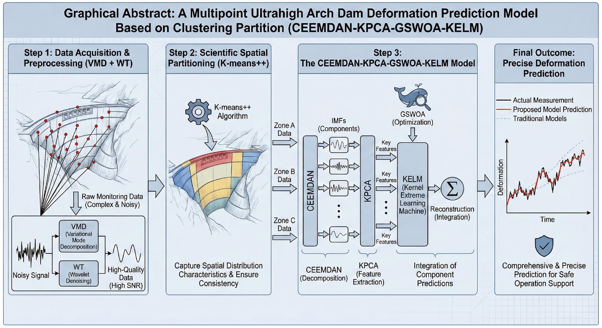
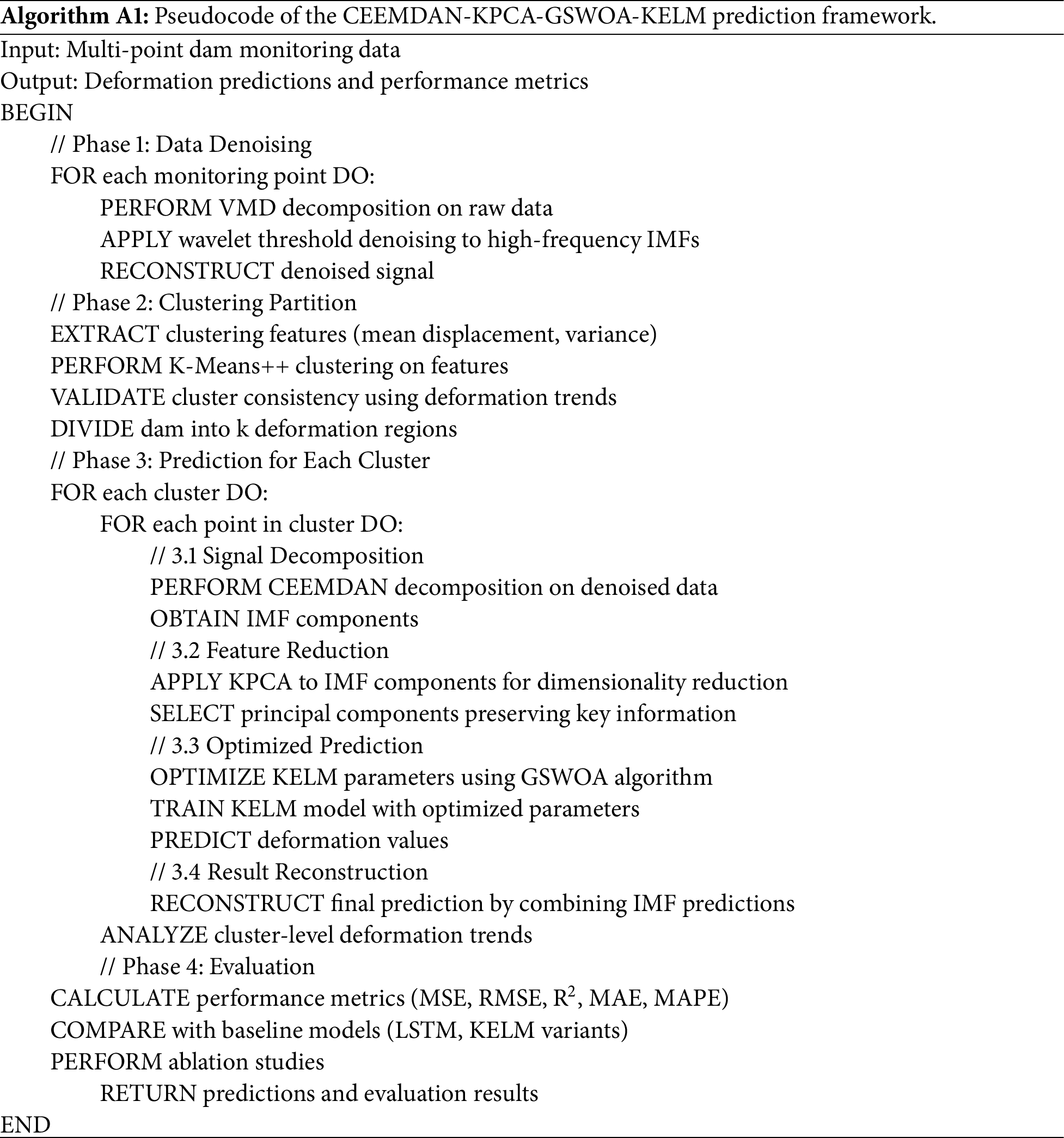
Deformation prediction for extra-high arch dams is highly important for ensuring their safe operation. To address the challenges of complex monitoring data, the uneven spatial distribution of deformation, and the construction and optimization of a prediction model for deformation prediction, a multipoint ultrahigh arch dam deformation prediction model, namely, the CEEMDAN-KPCA-GSWOA-KELM, which is based on a clustering partition, is proposed. First, the monitoring data are preprocessed via variational mode decomposition (VMD) and wavelet denoising (WT), which effectively filters out noise and improves the signal-to-noise ratio of the data, providing high-quality input data for subsequent prediction models. Second, scientific cluster partitioning is performed via the K-means++ algorithm to precisely capture the spatial distribution characteristics of extra-high arch dams and ensure the consistency of deformation trends at measurement points within each partition. Finally, CEEMDAN is used to separate monitoring data, predict and analyze each component, combine the KPCA (Kernel Principal Component Analysis) and the KELM (Kernel Extreme Learning Machine) optimized by the GSWOA (Global Search Whale Optimization Algorithm), integrate the predictions of each component via reconstruction methods, and precisely predict the overall trend of ultrahigh arch dam deformation. An extra high arch dam project is taken as an example and validated via a comparative analysis of multiple models. The results show that the multipoint deformation prediction model in this paper can combine data from different measurement points, achieve a comprehensive, precise prediction of the deformation situation of extra high arch dams, and provide strong technical support for safe operation.Graphic Abstract
Keywords
As of 2020, China has built over 90 thousand reservoirs and dams of all types, which play important roles in protecting people’s lives and promoting the social economy. However, concrete dams are subjected to natural forces and environmental erosion and experience material aging and high-pressure water seepage erosion, leading to the degradation of physical and mechanical properties and increasing safety hazards [1,2]. Dam deformation is an important norm for evaluating a dam’s safety, and it can intuitively show the integrity and stability of the structure. Thus, on the basis of concrete dam monitoring data, it is vital to build a highly accurate deformation prediction model, which would contribute to preventing potential risks and protecting people’s lives and property [3].
The dam safety monitoring model uses math, information science, intelligence algorithms, and other methods; it is based on a math model built from monitoring data; it is used for describing the dam situation, deformation rules, and causes; and then analyzes, predicts, and evaluates dam safety. The monitoring model was divided into three categories according to its development history: the regular model, emerging model, and intelligent computing model. The statistical model uses statistics to build a mathematical relationship between impact factors and effect size, but the parameters lack physical meaning and have a limited ability to fit complex nonlinear relationships [4]. The deterministic model estimates real physical parameters via the finite element method and builds monitoring data after optimized fitting, but it relies too much on the accuracy of finite base computing, making it sensitive to initial and boundary conditions. The mixed model combines the advantages of a statistical model and a deterministic model, and it can analyze and predict a dam’s safety situation; however, increased model complexity makes parameter selection and verification difficult [5]. The emerging model uses time series analysis [6], gray system theory [7], and other methods, builds single or composite patterns, and increases the prediction accuracy and model adaptation. However, increased model complexity makes computation, parameter selection, and verification difficult. With the advancement of computer technology and intelligent algorithms, machine learning models such as support vector machines [8,9], random forests [10,11], gray theory [12], and BP neural networks [13] have been widely used in dam deformation monitoring. The use of these models strongly improves the intelligence of dam monitoring because of their strong learning ability and nonlinear mapping capability. Scholars have successfully applied these techniques in the field of dam safety. For example, the nonlinear combination prediction model of extreme learning machines proposed by Cheng and Xiong [14] has performed well in dam displacement prediction. Refs. [15–17] combined a support vector machine with phase space reconstruction, wavelet analysis, and other methods and increased modeling efficiency and accuracy. Although machine learning models perform well in predicting performance trends at a single measurement point, many challenges remain in handling disturbing noise, addressing uneven spatial distributions of deformation, and determining model parameters. To increase the comprehensiveness and credibility of analyzing dam deformation trends, it is necessary to consider multiple angles and combine advanced theory and methods.
Regarding the complexity of dam deformation data, because the VMD can retain data trend features and increase information validity, it has been widely used [18–20]. For example, Sun et al. [21] proposed a GVLSTM model that utilizes Grey Wolf Optimization (GWO) to select the optimal parameters for VMD and combined it with LSTM, which effectively reduced estimation deviation and improved prediction stability. However, despite these improvements, VMD may still encounter issues such as overfitting or inadequate noise separation when analyzing highly complex non-stationary signals, resulting in the loss of useful information. Therefore, the current study combines VMD with wavelet denoising to process data. First, VMD divides the monitoring data into many modal components, considering that inaccuracies are concentrated on high-frequency components; then, wavelet denoising is used to denoise these high-frequency components precisely, improving the signal-to-noise ratio of the data. This method not only solves the VMD overfitting problem but also provides more precise import data for the subsequent dam deformation prediction model, increasing the accuracy and credibility of the prediction.
Furthermore, extra high arch dams, as large hydraulic concrete structures, are challenging to monitor because of their highly different deformation characteristics. The differences in the material parameters of the dam body, the large-span arch ring and the different regions resulted in different deformations, but the deformations at multiple measurement points in the same region were closely correlated. Cluster analyses, such as K-means, hierarchical clustering, and density peak clustering, are widely used in hydraulic safety monitoring; these methods can be used to effectively extract key information and delineate deformation areas precisely [22]. This work uses the K-means++ algorithm to optimize the initial clustering center selection, improve the clustering stability, and capture the characteristics of the zonal distribution of dam deformation precisely. CEEMDAN-KPCA technology adds adaptive noise to improve EMD via kernel principal component analysis; redundant information is removed, and key features are accurately extracted. Furthermore, the improved GSWOA [23] plays a key role in optimizing the KELM [24], significantly improving the model performance and convergence speed, and provides effective solutions for high-dimensional nonlinear problems. The combined application of these techniques provides strong support for the safe monitoring of extra high arch dams and ensures the accuracy and reliability of the monitoring results.
Most existing studies rely on single measurement point models or simple denoising techniques, which fail to fully capture the multi-point correlations and complex temporal patterns of dam deformation. These methods are sensitive to noise, unable to exploit multi-scale temporal features, and often yield limited predictive accuracy for extra high arch dams. To address these limitations, this paper proposes a multi-point integrated prediction framework for arch dam deformation based on spatiotemporally-informed clustering and advanced signal decomposition. The main research contributions are as follows:
(1) Noise elimination and data quality enhancement via VMD-WT denoising. By combining Variational Mode Decomposition (VMD) with Wavelet Transform (WT), monitoring data are preprocessed to remove noise and outliers, ensuring high-quality input for subsequent analysis.
(2) Adaptive measurement point zoning using K-Means++ clustering. Measurement points are partitioned based on deformation similarity, and the reasonableness of zoning is verified to ensure consistency of deformation trends within clusters, overcoming limitations of single-point analysis.
(3) A hybrid CEEMDAN-KPCA-GSWOA-KELM prediction model for multi-point forecasting. CEEMDAN decomposes the data into multiple intrinsic mode functions, KPCA reduces dimensionality and extracts key features, and the KELM network optimized via the GSWOA algorithm independently predicts each component. The final prediction integrates component results through reconstruction, accurately capturing overall deformation trends.
Together, this study introduces a comprehensive multi-point prediction framework that effectively addresses the deficiencies of traditional single-point models, providing a precise and reliable solution for deformation monitoring and safety assessment of extra high arch dams.
2.1 Variational Mode Decomposition
Variational mode decomposition (VMD) is a new signal decomposition method that decomposes the original signal into intrinsic mode functions (IMFs) of different frequencies, amplitudes, and phases, and more stable and controllable decomposition results are obtained via regularization constraints and iterative solving [25]. Compared with empirical modal decomposition (EMD) [26], the VMD algorithm has a more rigorous and complete mathematical theory, which can accurately explain the decomposition results; the decomposition results are more stable and controllable, and at the same time, the computational efficiency is greater. In the predictive framework established in this study, VMD serves not only as a key step for signal denoising but also as the foundation for subsequent deep feature extraction and modeling. By adaptively decomposing the original non-stationary displacement sequence into a series of intrinsic mode functions, VMD effectively separates high-frequency noise from feature components associated with different physical driving mechanisms. This structured multi-scale representation provides clearer and more informative inputs for the subsequent CEEMDAN-based refined decomposition, KPCA-based feature reduction, and partitioned prediction modeling, thereby ensuring the effectiveness and accuracy of characterizing the complex deformation behavior of the super-high arch dam. The specific method of VMD is as follows:
The modal split is processed to input signals using VMD, and a group of IMF components is obtained via continuous iteration. The set of k IMF components is
(1) For each IMF component, the analyzed signal associated with each mode is calculated via the Hilbert–Huang transform:
(2) An exponential term
(3) The demodulated signal is passed through H1 Gaussian smoothing to estimate the bandwidth of the signal. The variationally constrained problem is obtained, and the equations of this variationally constrained model are as follows:
where
For the variational problem, Lagrange multipliers
The alternating multiplier direction method is used to solve the above problem for the minimum value by iteratively updating
where
The specific decomposition process of the VMD algorithm is as follows: initialize
where
Wavelet denoising refers to the filtering of signals with noise under the wavelet transform to remove noise. Wavelet denoising is a method of filtering out noise and retaining the main features of the signal by processing the high-frequency wavelet coefficients (detail coefficients) by setting a threshold after performing the wavelet transform on the noisy signal [27]. Hard thresholding directly sets coefficients smaller than the threshold to zero, whereas soft thresholding reduces coefficients larger than the threshold, effectively removing high-frequency noise and retaining low-frequency useful information.
The main process of wavelet denoising is as follows:
(1) The wavelet coefficients are obtained by processing the wavelet transform of the original signals.
(2) For detailed coefficients, processing is performed according to certain threshold rules. Typically, a soft threshold or hard threshold is used, the soft threshold uses the shrinkage method and Bayesian method to compute the threshold, and the hard thresholds are processed as a set threshold.
(3) The wavelet is rebuilt to the above ratios, and the denoising signals are obtained.
(4) Optionally, the approximation coefficients are processed, and the same method of denoising is used for the high-frequency part.
(5) More accurate and stable data results are obtained through subsequent processing, such as prediction of the signal after denoising.
Currently used threshold functions include hard and soft threshold functions, and in this paper, the soft threshold method is selected to balance denoising and distortion.
Hard threshold function:
Soft threshold function:
where
2.3 Progress of the K-Means Clustering Algorithm
To overcome the limitations of global mixed modeling in multi-point deformation prediction and to effectively characterize the spatial heterogeneity of super-high arch dam deformation, this study first performs scientific zoning of monitoring points using cluster analysis. The aim is to group monitoring points with similar deformation trends into the same region so that subsequent prediction models can be constructed separately for each homogeneous zone, thereby capturing localized deformation patterns more accurately and improving overall prediction performance. On this basis, the K-means++ algorithm is employed to achieve cluster partitioning of monitoring points, and the principles and detailed procedures of the algorithm are described below. The k-means algorithm was proposed by J. MacQueen of Stanford University in 1967. This is a center point-based clustering algorithm, and the basic idea is to divide the data points into the centers of the nearest clusters so that the variance within the clusters is minimized. Currently, it is widely used in image processing and signal processing [28]. The input of the K-means algorithm is the number of cluster class centers
1. Initializing: Normalization of individual data.
2. Choose k cluster classes randomly
3. The cluster class to which each sample belongs is calculated according to the principle of minimizing the Euclidean distance, where the guidelines for the calculation are as follows:
where
For each cluster, recalculate its cluster center:
If a new cluster center is created, repeat steps two through four until the cluster center no longer changes.
This paper chooses the improved K-means++ algorithm to reduce the influence of the random position of initial center points on the clustering results. The criterion for selecting cluster center points for the K-means++ clustering algorithm is that the relative distance between the initial cluster centers is as far as possible [30]. The steps to confirm the initial cluster center are as follows:
Step 1: Confirming a cluster center
Step 2: Calculating the distance
Step 3: According to the weighted probability formula, the larger
Step 4: Repeat steps two and three until the number of k cluster center points has been selected.
2.4 Complete Ensemble Empirical Mode Decomposition with Adaptive Noise
The CEEMDAN algorithm is an improved adaptive noise-complete ensemble empirical modal decomposition method designed to improve the effectiveness of signal denoising and the accuracy of signal decomposition. It solves the problems of modal aliasing and noise that exist in traditional empirical modal decomposition (EMD) by introducing adaptive noise and complete integration strategies. Unlike traditional EMD, CEEMDAN introduces adaptive noise to improve the stability and accuracy of the decomposition, which reduces the errors generated during the decomposition process and improves the quality of the decomposition results [31]. In this study, CEEMDAN is employed to further decompose the denoised dam deformation data, generating a series of intrinsic mode functions (IMFs) with different physical interpretations, thereby providing a solid foundation for subsequent feature extraction. The specific steps are as follows:
In the CEEMDAN algorithm,
(1) When
(2) Gaussian white noise
(3) Similarly, for
(4) When the residual signal has no more than 2 extreme points, the residual signal cannot be further decomposed. When the CEEMDAN algorithm ends, a total of intrinsic modal functions are obtained, and the final residuals are:
Now, the raw deformation time series can be expressed as:
2.5 Kernel Principal Component Analysis (KPCA)
Due to the lack of a traditional PCA (Principal Component Analysis) algorithm, for nonlinearly separable data, the data cannot be correctly separated by a linear classifier in the original space. This leads to the proposal of improved principal component analysis, which uses a kernel function to map the data in a high-dimensional feature space, where the data can exhibit linearly separable properties [2]. In this study, KPCA is applied to perform nonlinear feature extraction and dimensionality reduction on the intrinsic mode functions (IMFs) generated by the CEEMDAN decomposition. The aim is to eliminate redundant information among modal components and condense the most effective feature set for deformation prediction, thereby improving the efficiency and accuracy of the subsequent forecasting model. The KPCA algorithm can be separated into the following steps:
(1) Calculating the kernel matrix K is:
where
(2) Centralized kernel matrix
The eigenvalue for the centralized kernel matrix is calculated and ordered by size
2.6 Optimization Techniques with WOA
The WOA (whale optimization algorithm) draws inspiration from the fascinating natural phenomena observed in whale behaviors and was presented by Mirjalili et al. from Griffith University, Australia, 2016 [32]. The algorithm achieves the solution of the optimization problem by simulating the feeding behavior of humpback whales in the ocean through phases such as searching, encircling, and spiraling to update their positions [20,33]. However, the WOA is not capable of performing a global search, and the accuracy of finding the optimal solution is relatively low. Therefore, in this paper, the GSWOA with a global search strategy is used [34]. In this study, GSWOA is employed to automatically optimize the kernel parameters and regularization coefficient of the KELM model, thereby enhancing the performance of the prediction model. The specific optimization of its algorithm is as follows:
(1) Adaptive weights: Add an inertia weight
where
where
where
(2) Variable Helix Position Update: When a whale searches for prey, it adjusts the distance traveled for each position update according to the shape of the helix between itself and the target point. Setting the parameter
(3) Optimal Field Fluctuation
In this position update process, the lower the number of optimal position updates is, the lower the algorithm search efficiency and convergence accuracy are. Therefore, this paper adopts the optimal domain fluctuation search to improve the convergence speed of the algorithm, and the formula is as follows:
where
The greedy algorithm is applied to the newly generated position to evaluate whether it should be retained, with the following formula:
where
2.7 Kernel Extreme Learning Machine (KELM) Algorithm
The kernel extreme learning machine (KELM) is a single hidden-layer feed-forward neural network algorithm characterized by the selection of random weights and thresholds. The KELM is unique in its method of randomly initializing these parameters between the input and hidden layers and within the threshold matrix of the hidden layer. This approach effectively solves the common problem in traditional backpropagation neural networks in which inappropriate initial weights and thresholds often lead to suboptimal local solutions [35]. In this study, KELM is selected as the final predictor owing to its outstanding performance and efficiency in handling small-sample and nonlinear regression problems.
As shown in Fig. 1, this model is constructed in three parts: the input layer, hidden layer and output layer. The basic principle is as follows: suppose that the set of input data is
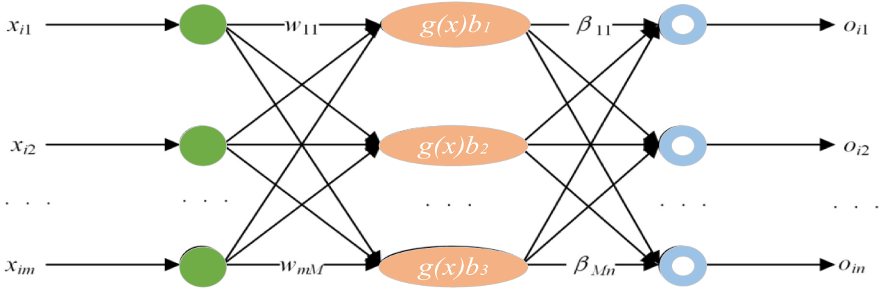
Figure 1: KELM structure schematic.
If the ELM (Extreme Learning Machine) with a single hidden layer is able to approximate the “
where
The ELM is a single hidden-layer feed-forward neural network whose stochastic nature of weights and biases leads to fluctuating predictions. To improve this, the kernel extreme learning machine (KELM) is proposed by adding regularization and kernel tricks [36–38] where
The KELM optimizes the regularization parameter C to minimize the training error and control the output weight paradigm to enhance model generalization and prevent overfitting. At this time, the output weights
For the unknown situation to hidden layer feature mapping
The output function of the KELM is as follows:
where
To overcome the limitations of the traditional unilateral point model, this paper proposes a comprehensive model that integrates VMD-WT noise reduction, K-Means++ clustering, and CEEMDAN-KPCA-GSWOA-KELM prediction techniques. The detailed process shown in Fig. 2 includes the following steps:
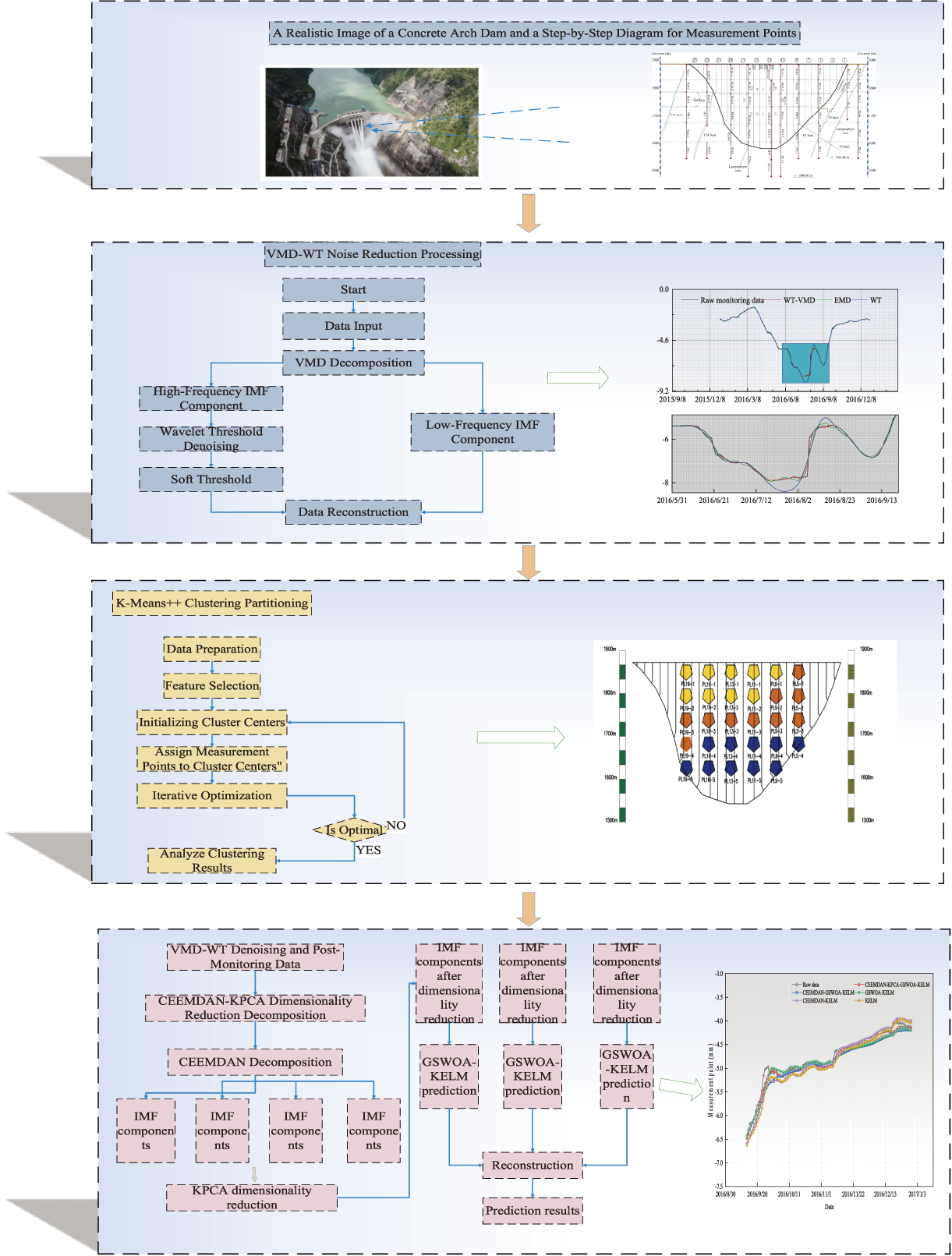
Figure 2: Model flow chart.
Step 1. Denoising dam monitoring data via VMD-WT.
The dam deformation data are first decomposed using the VMD method. This process generates modal functions and their spectra and center frequencies, which lay the foundation for further analysis. The initial VMD parameters are set as follows: the number of decomposition layers (K) is set to 7, the penalty factor α is set to 1000, and the initial center frequency is randomly selected, but it is set to 1 as the starting point in this example.
Second, after the modal function from the VMD is obtained, the wavelet threshold noise reduction method is used to reduce the high-frequency components, and finally, the noise-reduced high-frequency IMF components are reconstructed with the low-frequency components to obtain the noise reduction and data. The specific parameters of wavelet thresholding noise reduction are set as follows: db6 is used as the wavelet basis function, and the number of decomposition layers is set to 3. However, a noise standard deviation of 0 may mean that no additional noise is added to the signal, which may need to be adjusted according to the specific situation in practical applications.
Step 2. K-means clustering algorithm for dam partitioning
The preprocessed 3D feature data are first analyzed by clustering using the K-Means++ algorithm. This process assigns the data points to different clusters, which provides the basis for further analysis and application. The specific initial parameters are set as follows: the number of clusters (K) is set to 3, and the center of mass is initialized via the K-Means++ method. According to the results after clustering combined with the deformation trend of the original data measurement points, the division of the deformation region of the dam is reasonably verified.
Step 3. CEEMDAN-KPCA-GSWOA-KELM model’s prediction for measurement points.
The core of Step 3 is to construct an arch dam deformation prediction model based on the CEEMDAN-KPCA-GSWOA-KELM using the data processed via VMD-WT noise reduction. This step is divided into the following steps:
(1) Normalization of the VMD-WT noise-reduced data.
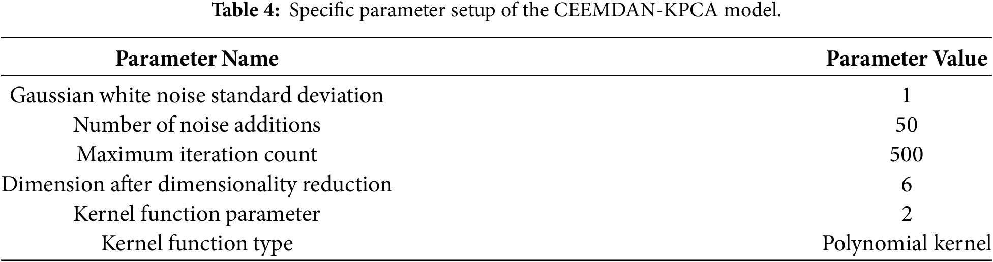
(2) CEEMDAN-KPCA is applied to reduce the dimensionality of the monitoring data after noise reduction, and the initial parameters of the model are set as follows: the standard deviation of the Gaussian white noise is 1, the number of added noises is 50, the maximum number of iterations is 500, the dimension of the reduced dimensionality is 6, the kernel function parameter is 2, and the type of kernel function is a polynomial kernel function.
(3) Setting the parameters of the GSWOA-KELM model.
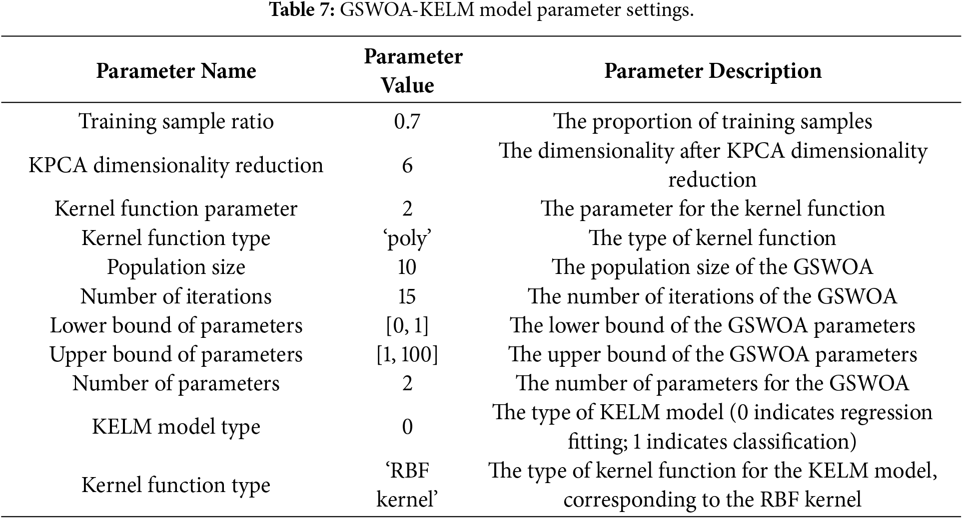
(4) By optimizing the GSWOA, the optimal weights and fitness values of the KELM model can be determined. The specific initial parameters of the model are set as follows: the proportion of training samples is 0.7, the population size is 10, the number of iterations is 15, the lower bound of the parameters of the GSWOA is [0,1], the upper bound is [1,100], the number of parameters of the GSWOA is 2, the type of KELM model is 0 (0 means regression, 1 means classification), and the kernel function is ‘RBF_kernel’.
(5) Finally, the prediction of multiple measurement points in the subarea is carried out to synthesize and analyze the overall trend and law of change to assess the safety status of the dam.
The main research object of this project is located at the junction of Yanyuan County and Muli County in Liangshan Prefecture, Sichuan Province. It is a mega concrete double-curvature arch dam with a design dam height of 305 m; it is the highest double-curvature thin-arch dam in the world that has been built or is under construction or is in design, and its level of construction difficulty is rare worldwide (Fig. 3). This is due mainly to the concrete hyperbolic arch dam (including the plunge pool and secondary dam), the right bank spillway hole, the right bank diversion power generation system and switching station, etc., as well as the existing buildings on the left bank for the diversion hole and its construction branch hole. The engineering grade is I, and the main hydraulic building is level 1. The normal water level of the reservoir is 1880 m, the dead water level is 1800 m, the storage capacity below the normal water level is 7.765 billion cubic meters, and the regulating capacity is 4.91 billion cubic meters, which is an annual regulating reservoir. The power station has 6 installed units, with a single capacity of 600 MW.
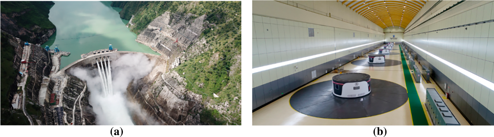
Figure 3: Dam profile. (a) Aerial view of the dam; (b) Internal view of the dam.
To ensure the safety and optimal performance of the hydropower plant, a series of comprehensive monitoring systems has been implemented since the start of the project. These include an automatic dam safety monitoring system, a GNSS (Global Navigation Satellite System)-based dam top deformation monitoring system, a 3D laser measurement system, a dynamic monitoring system for the seismic response of dams and a strong earthquake monitoring system. These systems are connected to multiple measurement points, including deformation monitoring, crack monitoring, seepage monitoring, temperature monitoring and satellite monitoring. This paper focuses mainly on deformation monitoring. Therefore, 29 monitoring points specializing in deformation monitoring are selected in this paper. The detailed layout of these monitoring instruments is shown in Fig. 4.
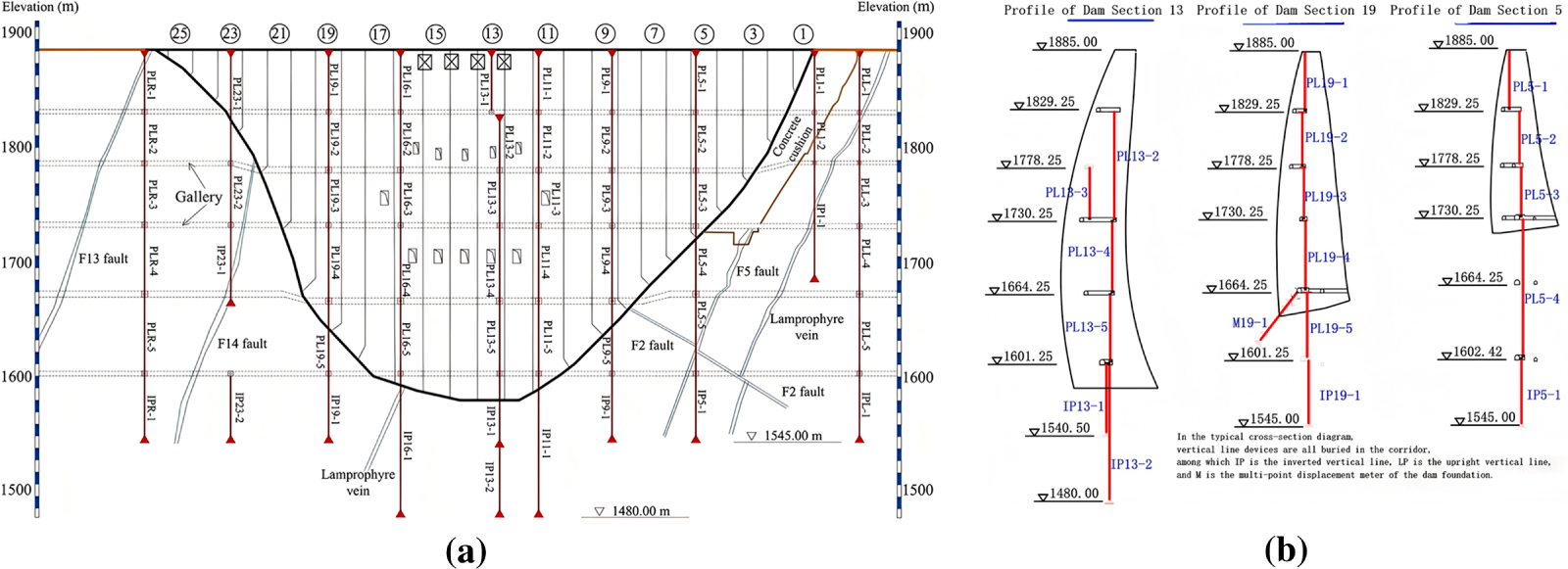
Figure 4: Arch dam vertical monitoring arrangement. (a) Overall layout; (b) Detail picture.
To avoid the influence of residual missing values on the model, monitoring data from 2016–2017 with high data integrity were selected as samples in this study to better reflect the deformation of the dam under different water level and air temperature conditions. For the selected monitoring dataset, a few measurement points contain sporadic missing records at individual time steps. To ensure the continuity of the time series and to minimize potential bias in subsequent decomposition and prediction modeling, this study employs a time-series-based linear interpolation method to fill the missing values. This approach utilizes the valid measurements immediately before and after the missing entries for linear estimation, effectively preserving the local deformation trend. Accordingly, it is considered a reasonable and efficient strategy for handling missing data in equally spaced monitoring sequences. The specific water level and air temperature are shown in Fig. 5 below:
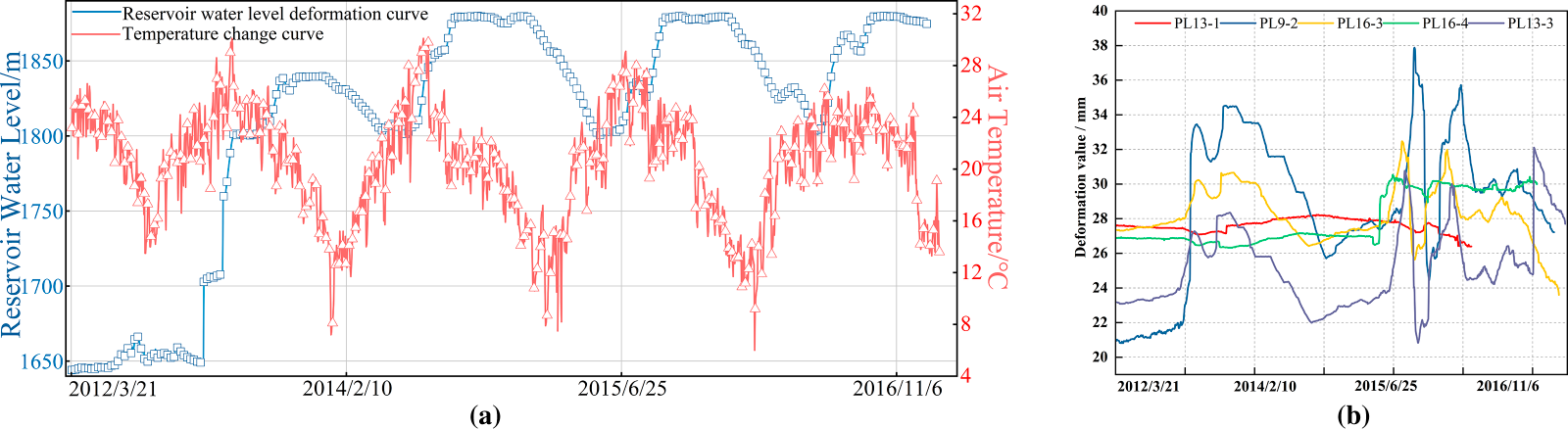
Figure 5: Water level, water temperature and deformation process diagram (a) Reservoir levels, temperature process lines; (b) Process line for monitoring the horizontal displacement of the dam section.
4.2 Multi-Measurement Point Clustering Partitions Considering Spatial Correlations
To construct the dam deformation prediction model with multiple measurement points, this paper calculates the mean relative displacement, average relative displacement, and variance of 29 measurement points by taking them as the clustering features of the measurement points. It is clustered via the K-Means++ clustering method, and the dam is reasonably divided into regions according to the clustering results of the measurement points. The specific clustering features are shown in Table 1 below.
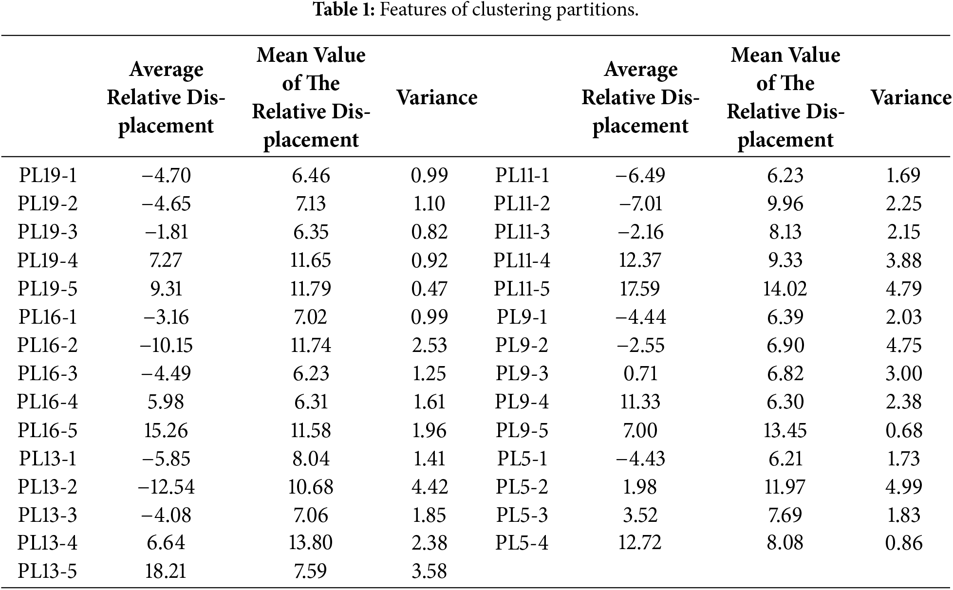
The average relative displacement is defined as the average value of the absolute values of the displacement differences of each measurement point with respect to all other measurement points at multiple time points. It reflects the average extent of the position changes among the measurement points at different time points, demonstrating the deformation trend of the measurement points themselves as well as their relative movements with respect to other measurement points. The mean value of the relative displacement is the average value of the absolute values of the displacement differences of each measurement point with respect to all other measurement points at multiple time points. It reflects the relative positional relationship among the measurement points. The standard deviation reflects the degree of dispersion of the displacement data of the measurement points, that is, the extent to which the displacement data deviates from their average value. The specific clustered measurement point partition is as follows:
As shown in Fig. 6, the deformation area of the dam was divided into three zones on the basis of the clustering results: PL19-1, PL16-1, PL13-1, PL11-1, PL9-1, and PL5-1 as Zone 1; PL19-2, PL16-2, PL13-2, PL11-2, PL9-2, and PL5-2 as Zone 2; and PL19-3, PL16-3, PL13-3, PL11-3, PL9-3, and PL5-3 as Zone 3.
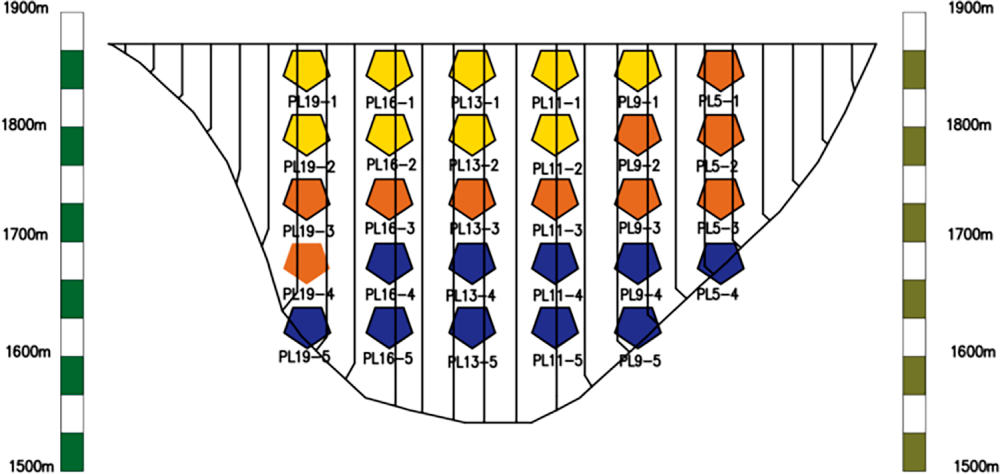
Figure 6: Clustering partition of arch dam measurement points.
To validate the rationality of the selected cluster number, comparative experiments were conducted using different cluster quantities, and clustering evaluation metrics including the average silhouette coefficient, Calinski-Harabasz index, and Davies-Bouldin index, were calculated. The specific results are shown in Table 2 below:
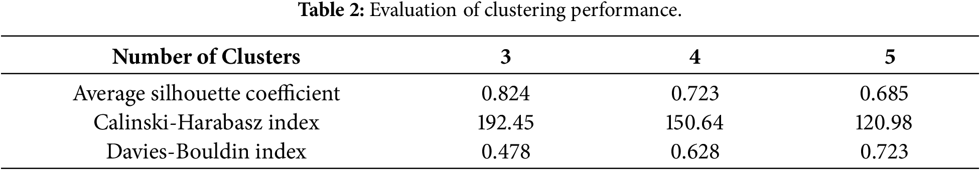
The results indicate that when the number of clusters is set to three, the average silhouette coefficient reaches its maximum, the Calinski–Harabasz index is the highest, and the Davies–Bouldin index reaches its minimum, suggesting higher intra-cluster compactness, greater inter-cluster separability, and the best overall clustering performance. Therefore, selecting three clusters most appropriately reflects the intrinsic structure of the data. This clustering partition exhibits clear correspondence with the physical configuration and stress characteristics of the arch dam. Based on the spatial distribution of monitoring points and the dam’s mechanical behavior, Zone 1 primarily covers the upper region of the dam and both abutments, where deformation is strongly influenced by water level fluctuations and abutment constraints. Zone 2 corresponds to the arch crown beam and its adjacent area, where deformation is mainly governed by the global arch action and periodic thermal effects. Zone 3 is concentrated in the middle and lower sections of the dam, where deformation is jointly controlled by foundation constraints and hydrostatic pressure. Thus, the clustering results effectively represent distinct deformation patterns associated with the crown-beam zone, the abutment-influenced zone, and the mid-lower foundation-controlled zone, providing a physically interpretable basis for subsequent sub-regional modeling. To further validate the rationality of the zoning, sampling points from Zone 1 were selected as analysis objects. By plotting the relative deformation trends of the corresponding monitoring points, the effectiveness of the partitioning can be visually and quantitatively evaluated. The results are shown in the figure below (Fig. 7).
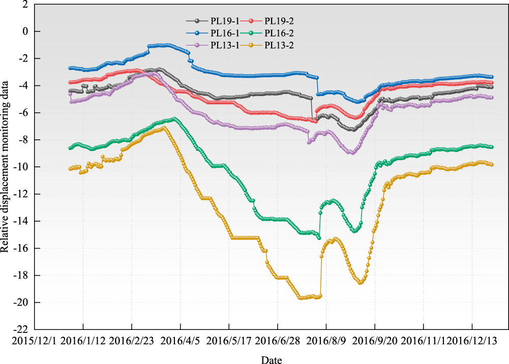
Figure 7: Deformation trends at each measurement point in Zone 1.
As seen from the relative deformation trend graphs for each measurement point of the dam shown in Fig. 7 above, the relative displacement monitoring data for the six measurement points (PL19-1, PL19-2, PL16-1, PL16-2, PL13-1, and PL13-2) have roughly the same trend over the time span. Specifically, the deformation trends at all the measurement points experienced a downward and then an upward trend and reached the minimum around August 2016, followed by a gradual recovery. Although the specific deformation values of each measurement point differed in different time periods, the overall trend and direction of fluctuation were essentially the same.
4.3 Data Noise Reduction Based on WT-VMD Models
To ensure the causality of time-series prediction and prevent data leakage, a strict data processing protocol was implemented in this study. First, the monitoring data were chronologically divided into training and testing sets. All denoising and feature extraction procedures were strictly performed on the training set only. To improve the accuracy of dam deformation prediction and to verify the effectiveness of the WT-VMD noise reduction model, the relative displacement data of the PL13-3 measurement point were selected for model comparison and verification in this study. The detailed parameter configurations of the WT-VMD model are shown in the table below (Table 3), and the comparison graph of the noise reduction effect is shown in the following figure.
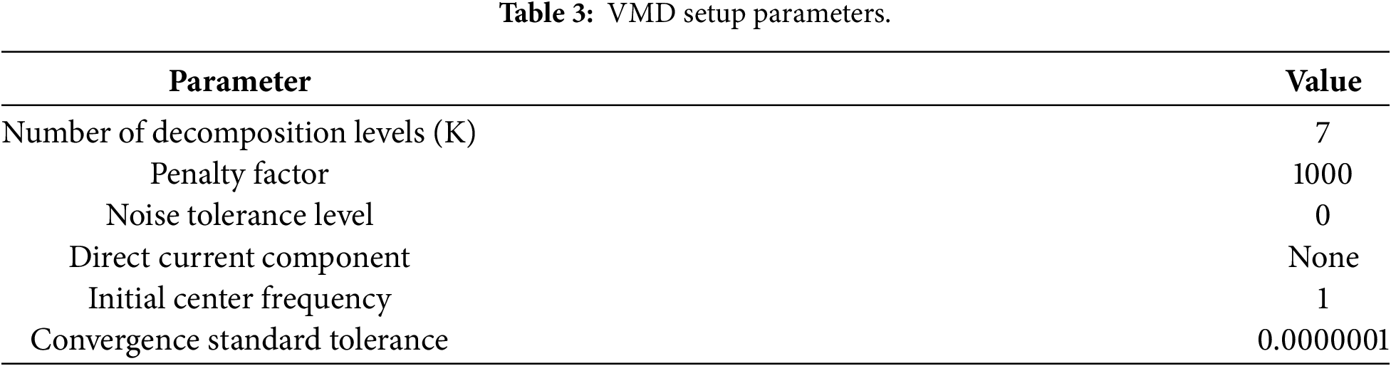
Fig. 8 shows the results of VMD and WT-VMD for processing the dam monitoring data after an in-depth comparison of the effects of the three noise reduction methods of WT, and the advantages and limitations of each method can be clearly observed. The wavelet thresholding method is particularly good at smoothing peaks and valleys, but its thorough noise reduction leads to the loss of some original data features, making its noise reduction curve significantly different from that of the original data. The VMD noise reduction method retains more original data features by finely decomposing the signals and removing the high-frequency IMF components to reconstruct the low-frequency signals, but the important data features embedded in the high-frequency IMF components are directly removed, which may lead to incomplete elimination of noise and noise. The WT-VMD method combines the advantages of the wavelet transform and VMD, first decomposes the signal via VMD and then denoises the high-frequency IMF components and reconstructs them, which successfully retains the core features of the original data and more finely handles the noise errors in the peaks and valleys to achieve better noise reduction, thereby providing accurate and reliable data for subsequent data preprocessing and deformation prediction. support.
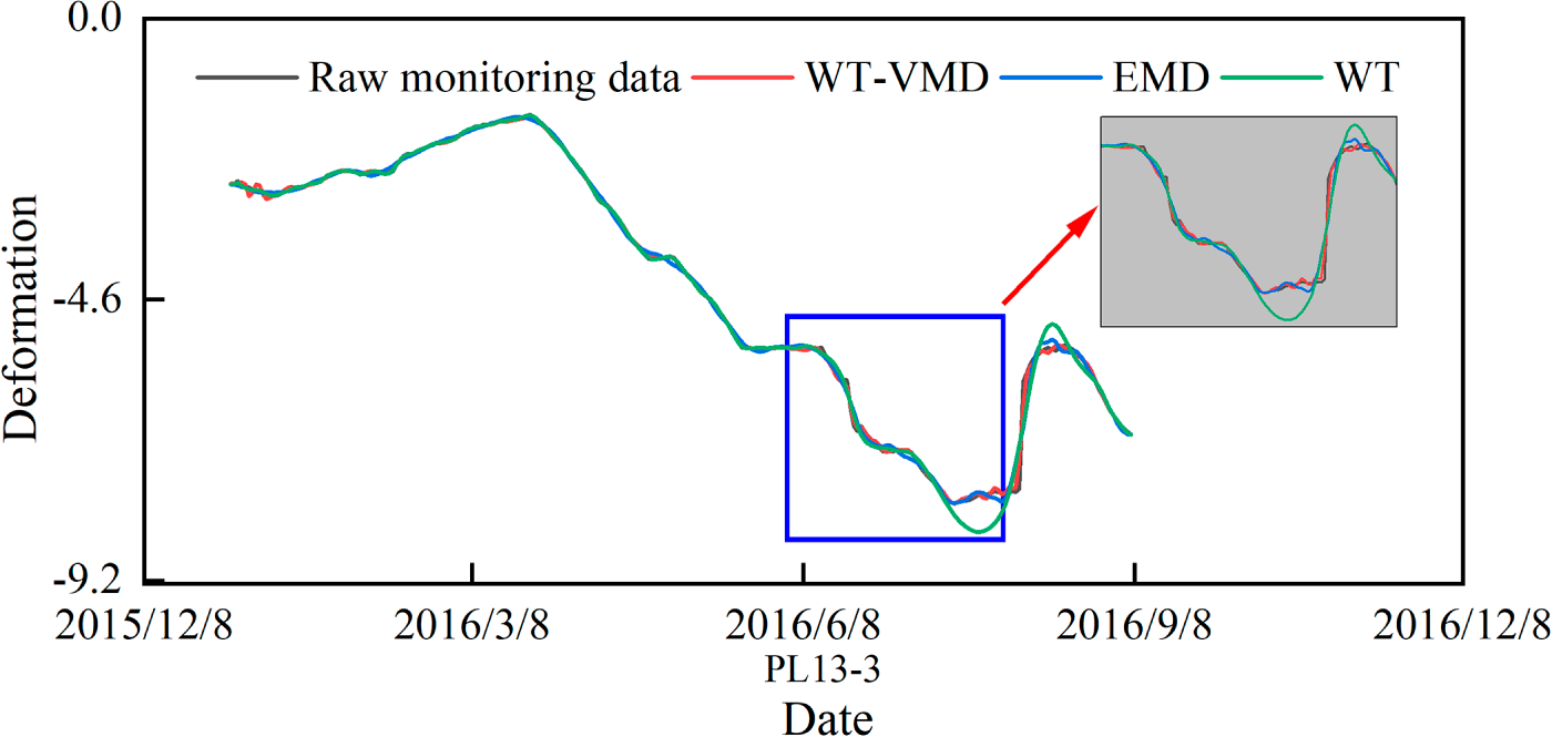
Figure 8: Monitoring values after VMD-WT noise reduction at measurement point PL13-3.
4.4 Multi-Measurement Point Prediction Based on the CEEMDAN-KPCA-GSWOA-KELM
4.4.1 CEEMDAN-KPCA Data Decomposition and Dimensionality Reduction
To overcome the limitations of noise interference and insufficient feature extraction in traditional data processing methods, this paper applies the CEEMDAN technique to decompose the data finely and successfully generates multiple modal components with unique data characteristics. The KPCA technique is subsequently applied to downscale these modal components to eliminate redundant information and accurately extract key features. This method not only improves the efficiency and accuracy of data processing but also provides a more reliable basis for subsequent data analysis and prediction, which helps to realize an in-depth understanding and accurate prediction of complex systems such as dam deformation. Owing to the heavy weight of measurement points, this paper takes measurement point PL19-1 as an example, and the specific CEEMDAN-KPCA model parameters are as follows (Table 4) [39,40]:
As shown in Fig. 9, the IMF components obtained through CEEMDAN decomposition exhibit clear physical significance. Generally, the low-frequency IMF (e.g., IMF1) varies slowly with a long period, primarily reflecting the quasi-static response of the dam induced by reservoir water pressure, as well as time-dependent effects such as concrete creep. The mid-frequency IMFs (e.g., IMF2–IMF4) show distinct periodic oscillations, with periods corresponding to annual or seasonal cycles, which mainly represent thermal expansion and contraction of the dam caused by periodic temperature variations. In contrast, the high-frequency IMFs feature small amplitudes and rapid fluctuations, containing measurement noise and short-term environmental disturbances. This frequency-driven physical separation mechanism provides a solid basis for subsequent refined prediction modeling targeting different driving factors.
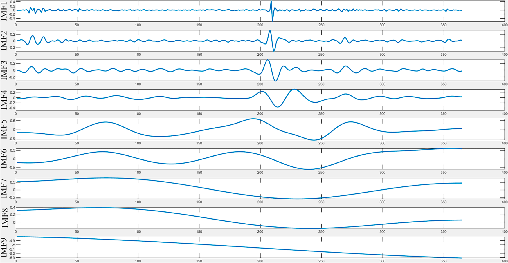
Figure 9: IMF components decomposed by CEEMDAN.
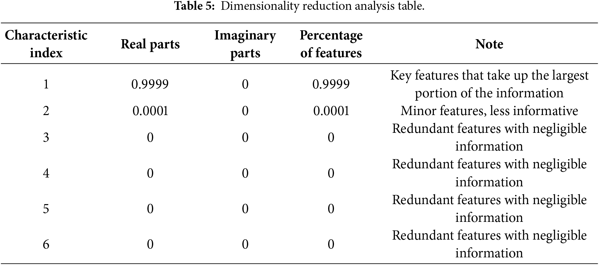
In this paper, the KPCA algorithm is used to perform dimensionality reduction on the IMF components obtained from decomposition, and a series of experimental validations show that 6 dimensions is the best dimensionality reduction. An in-depth analysis of the feature dimensionality reduction analysis table (Table 5) reveals that the first feature accounts for almost all of the information, up to more than 99%, whereas the information contributed by other features is negligible and can almost be ignored. This indicates that the first feature is the core key feature that dominates the information direction of the whole dataset. Therefore, this dimensionality reduction process not only effectively retains the information of the key features but also drastically reduces the amount of redundant information, which makes the data after dimensionality reduction more concise and representative.
To verify the effectiveness of GSWOA-optimized KELM, this study takes the PL19-1 monitoring point dataset as an example and conducts comparative experiments with several commonly used meta-heuristic algorithms, including PSO (Particle Swarm Optimization), GA (Genetic Algorithm), and the original WOA. All algorithms are executed under identical parameter settings to optimize the PL19-1 dataset, and the evaluation is performed using multiple performance metrics. The experimental results are shown as follows (Table 6).
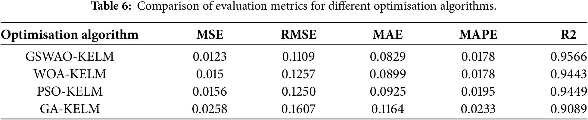
As shown in the table, GSWOA-KELM outperforms WOA-KELM, PSO-KELM, and GA-KELM across multiple performance metrics. In particular, it demonstrates remarkable advantages in key regression indicators such as MSE (0.0123), RMSE (0.1109), and R2 (0.9566). This indicates that GSWOA-KELM is more effective in reducing prediction error and achieving a better fit to the data. GSWOA is an improved optimization method based on the Grey Wolf Optimizer (WOA), incorporating optimal neighbourhood perturbation, adaptive weighting, and variable-spiral position updating mechanisms. Compared with traditional WOA, PSO, and GA, it achieves a better balance between global and local search capabilities, effectively avoiding local optima and enhancing optimization accuracy and efficiency. Therefore, the proposed KELM prediction model is optimized using GSWOA in this study.
4.4.2 Multimeasurement Point Prediction for the CEEMDAN-KPCA-GSWOA-KELM Model
Through an in-depth analysis of the decomposition and dimensionality reduction results of the CEEMDAN-KPCA model, it is observed that the dimensionality reduction process effectively preserves the key features of the data while significantly eliminating redundant information. This optimized data representation provides a more efficient and accurate foundation for subsequent processing and prediction tasks. Based on this, a KELM model optimized by GSWOA and integrated with CEEMDAN-KPCA (i.e., CEEMDAN-KPCA-GSWOA-KELM) is proposed to enhance the monitoring and forecasting performance of dam deformation systems.
To further improve prediction accuracy, the partitioning results previously obtained are incorporated, and the noise-reduction capability of the WT-VMD model is utilized. Meanwhile, reservoir water level, temperature, and other key deformation-driving factors are introduced as input variables for the prediction model. In the model comparison experiments, all models were trained and tested under the same data division scheme, with 70% of data used for training and 30% for testing. Consistent input and output features were maintained across all models to ensure fairness and scientific validity of the comparison results. Based on this methodology, annual data from 2016–2017 were used to perform predictions for multiple monitoring points in Zone 1, verifying the superiority of the proposed CEEMDAN-KPCA-GSWOA-KELM model in dam deformation prediction. The specific configuration of model parameters is as follows (Table 7) [41,42]:
To verify the superiority of the CEEMDAN-KPCA-GSWOA-KELM model in dam deformation prediction, comparative analyses of the CEEMDAN-GSWOA-KELM, GSWOA-KELM, CEEMDAN-KELM, and KELM models were conducted in this study. This comparative analysis focuses on the denoised Zone 1 dam monitoring data from the VMD-WT model, which helps highlight the advantages of the CEEMDAN-KPCA-GSWOA-KELM model. The prediction curves for each model are shown in Fig. 10, and the residuals of the prediction models are shown in Fig. 11.
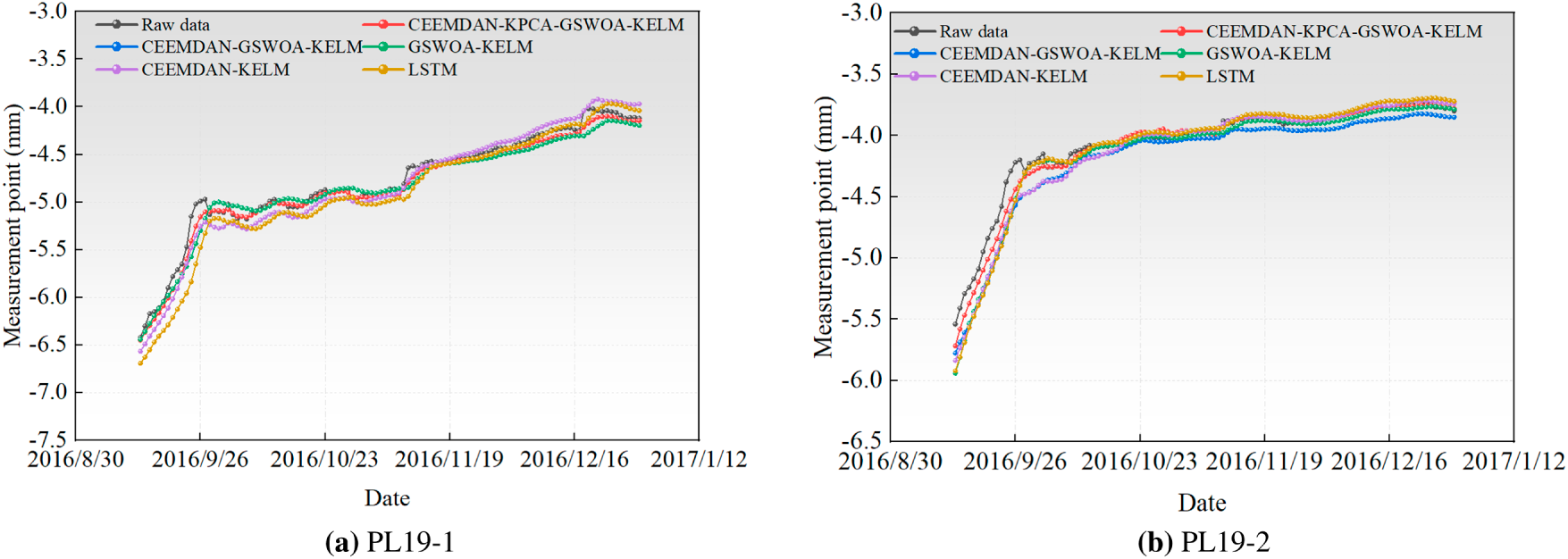
Figure 10: Comparison of the prediction results by measurement points in Zone 1. (a) PL19-1. (b) PL19-2.
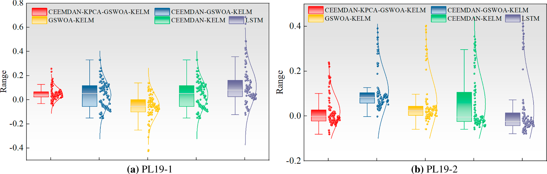
Figure 11: Residual boxplots of the predictive model for each measurement point in Zone 1. (a) PL19-1. (b) PL19-2.
The performance and accuracy of the models were comprehensively assessed via five key metrics: goodness of fit (R2), root mean square error (RMSE), mean absolute error (MAE), mean absolute percentage error (MAPE), and mean square error (MSE). Specifically, the R2 metric reflects the model’s goodness of fit to the data, the RMSE represents the average deviation between the model’s predicted and true values, the MAE represents the average of the absolute values of the prediction errors, the MAPE represents the average level of prediction error in percentage form, and the MSE represents the mean square error of the model’s predicted values. See Table 8 and Fig. 12 for detailed model prediction results. The prediction results for other measurement points are presented in Appendix A.
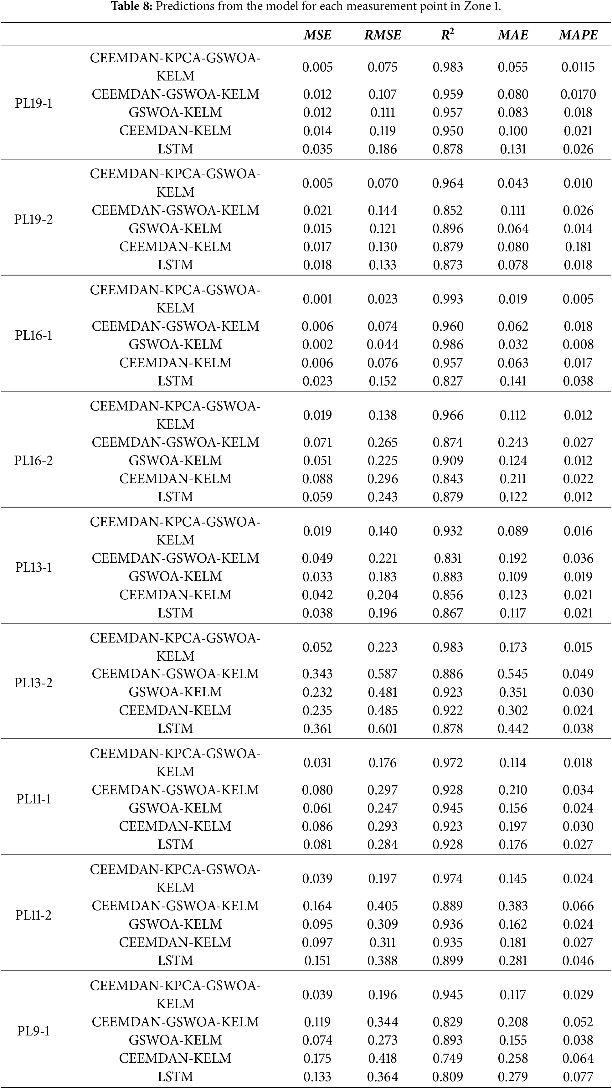
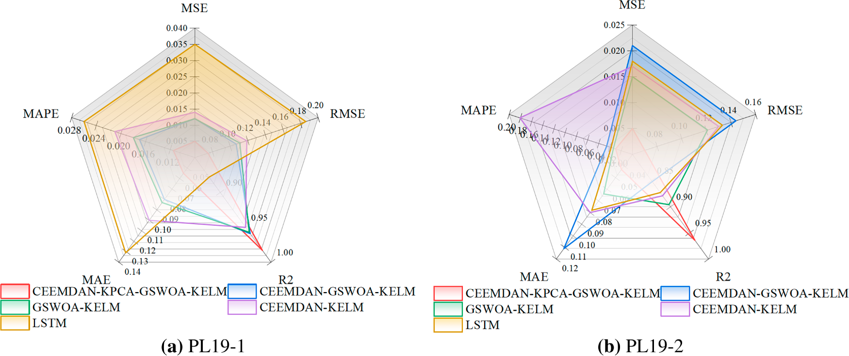
Figure 12: Model evaluation metrics for each measurement point in Zone 1. (a) PL19-1. (b) PL19-2.
As shown in Figs. 10 and 11 above, the CEEMDAN-KPCA-GSWOA-KELM model performs well compared with the other models at multiple measurement points. Taking the PL19-1 measurement point as an example, the CEEMDAN-KPCA-GSWOA-KELM model showed significant performance advantages over the other control models. As shown in the radar chart of evaluation indicators for measurement points in Fig. 12, this model shows an improvement in the R2 metric of approximately 0.024, 0.026, 0.033, and 0.105 compared to CEEMDAN-GSWOA-KELM, GSWOA-KELM, CEEMDAN-KELM, and LSTM, respectively. This indicates that the CEEMDAN-KPCA-GSWOA-KELM model is better at capturing the relationships and trends within the data. The model also excels in other evaluation metrics. The improvement in the MSE metric is 0.007, 0.007, 0.009, and 0.030, respectively. The improvement in the RMSE metric is 0.032, 0.036, 0.044, and 0.111, respectively. The improvement in the MAE metric is 0.025, 0.028, 0.045, and 0.076, respectively. The reduction in the MAPE metric is 0.0055, 0.0065, 0.0095, and 0.0145, respectively. These results indicate that the CEEMDAN-KPCA-GSWOA-KELM model has a clear advantage in reducing prediction errors and improving prediction accuracy.
In the proposed model, the synergistic effect of CEEMDAN and KPCA remarkably enhances prediction performance. CEEMDAN conducts multi-scale decomposition of the original signal, effectively extracting local component features and suppressing noise, thereby improving the model’s ability to capture nonlinear and non-stationary characteristics. KPCA, through kernel mapping, projects the data into a higher-dimensional feature space and performs nonlinear dimensionality reduction, which preserves the intrinsic nonlinear structure of the data while eliminating redundant information and reducing the risk of overfitting. The combination of CEEMDAN and KPCA thus optimizes both feature extraction and model learning, leading to a substantial improvement in prediction accuracy.
In addition, Fig. 12 shows that the CEEMDAN-KPCA-GSWOA-KELM model has the smallest fluctuation of residual values across multiple measurement points, for example, at the PL19-1 measurement point, which is usually in the range of [−0.25, 0.25], compared with the residual values of the CEEMDAN-GSWOA-KELM, GSWOA-KELM, and LSTM models. This fluctuation is significantly smaller. This result indicates that the model provides stable and accurate predictions with reduced prediction errors, which increases the credibility of the model. This low residual fluctuation ensures that the model outputs predictions with high confidence intervals, which provides strong data support for the monitoring of dam deformation.
In summary, the proposed CEEMDAN-KPCA-GSWOA-KELM model demonstrates superior performance across multiple monitoring points compared with the other benchmark models. Its outstanding evaluation metrics and effective control of residual fluctuations not only confirm its strong capability in capturing deformation patterns and improving prediction accuracy, but also produce smooth, continuous, and physically consistent prediction curves. These characteristics provide a direct and reliable reference for deformation safety monitoring in practical engineering applications. Moreover, no abnormal mutation trend is observed in the prediction results, indicating that the dam remains in a stable state during the forecast period, and thus the model output can serve as a credible baseline for future monitoring, facilitating early detection of deformation anomalies and safety assessment.
In this study, a comprehensive research model is constructed to accurately predict and deeply analyze the deformation trend of extra-high arch dams. The model incorporates the fusion of variational modal decomposition (VMD) with wavelet threshold noise reduction (WT) technique, K-Means++ algorithm, and CEEMDAN-KPCA-GSWOA-KELM model. The monitoring data were first preprocessed by the VMD-WT model, which significantly improved the signal-to-noise ratio of the data and laid a solid foundation for the subsequent analysis. Subsequently, the K-Means++ algorithm was used for scientific clustering and partitioning, which accurately captured the spatial distribution characteristics of the deformation of the extra-high arch dam and ensured the consistency of the deformation trend of the measurement points within the partition.
In the prediction stage, the monitoring data are decomposed by the CEEMDAN technique, which effectively extracts the different modal components of the signal and improves the accuracy and stability of the decomposition by adaptively adjusting the noise. Subsequently, KPCA is used to downscale the IMF components, eliminating redundancy and retaining the core features to improve the prediction efficiency and accuracy. The GSWOA algorithm then optimizes the KELM model parameters to achieve the optimal configuration through its excellent search and convergence capabilities. For each dimensionality-reduced IMF component, the KELM model predicts independently to ensure the high relevance and accuracy of the prediction results. Finally, by reconstructing the prediction results of each IMF component, the accurate prediction of the deformation trend of the extra-high arch dam is realized, which provides strong technical support for the dam safety management. Although the model has achieved significant results in deformation prediction, its limitations need to be recognized. In particular, the VMD method may face challenges when dealing with extremely complex signals and requires further improvement in future research. Accordingly, new intelligent algorithms should be explored to enhance monitoring data processing techniques, and innovative data acquisition techniques should be developed to collect higher-quality and more comprehensive monitoring data to improve the model’s ability to handle complex signals.
In the future, research will focus on optimizing the CEEMDAN-KPCA-GSWOA-KELM model and exploring new intelligence algorithms and data collection technologies. In addition, more reasonable cluster partitioning for dam deformation should be performed, the features of the zonal distribution of dam deformation should be captured precisely, and the consistency of the deformation trends of the measurement points should be ensured. Future studies will provide more accurate, reliable, and applicable solutions for analyzing deformation trends in arch dams, thereby enhancing their safety and operational integrity.
Acknowledgement: Not applicable.
Funding Statement: This study was supported by the National Natural Science Foundation of China (Grant Nos. 52069029, 52369026); the Belt and Road Special Foundation of National Key Laboratory of Water Disaster Prevention (Grant No. 2023490411); the Yunnan Agricultural Basic Research Joint Special General Project (Grant Nos. 202501BD070001-060, 202401BD070001-071); Construction Project of the Yunnan Key Laboratory of Water Security (No. 20254916CE340051) and the Youth Talent Project of “Xingdian Talent Support Plan” in Yunnan Province (Grant No. XDYC-QNRC-2023-0412).
Author Contributions: The authors confirm contribution to the paper as follows, Bin Ou: formal analysis, investigation, methodology, software, validation, visualization, writing-original draft. Haoquan Chi: data curation, writing—review and editing. Xu’an Qian: methodology, software. Shuyan Fu: formal analysis, investigation. Zhirui Miao and Dingzhu Zhao: data curation, validation. Bin Ou: funding acquisition, project administration, resources, and writing—review and editing. All authors reviewed and approved the final version of the manuscript.
Availability of Data and Materials: The datasets analyzed during the current study are available from the corresponding author upon reasonable request.
Ethics Approval: Not applicable.
Conflicts of Interest: The authors declare no conflicts of interest.
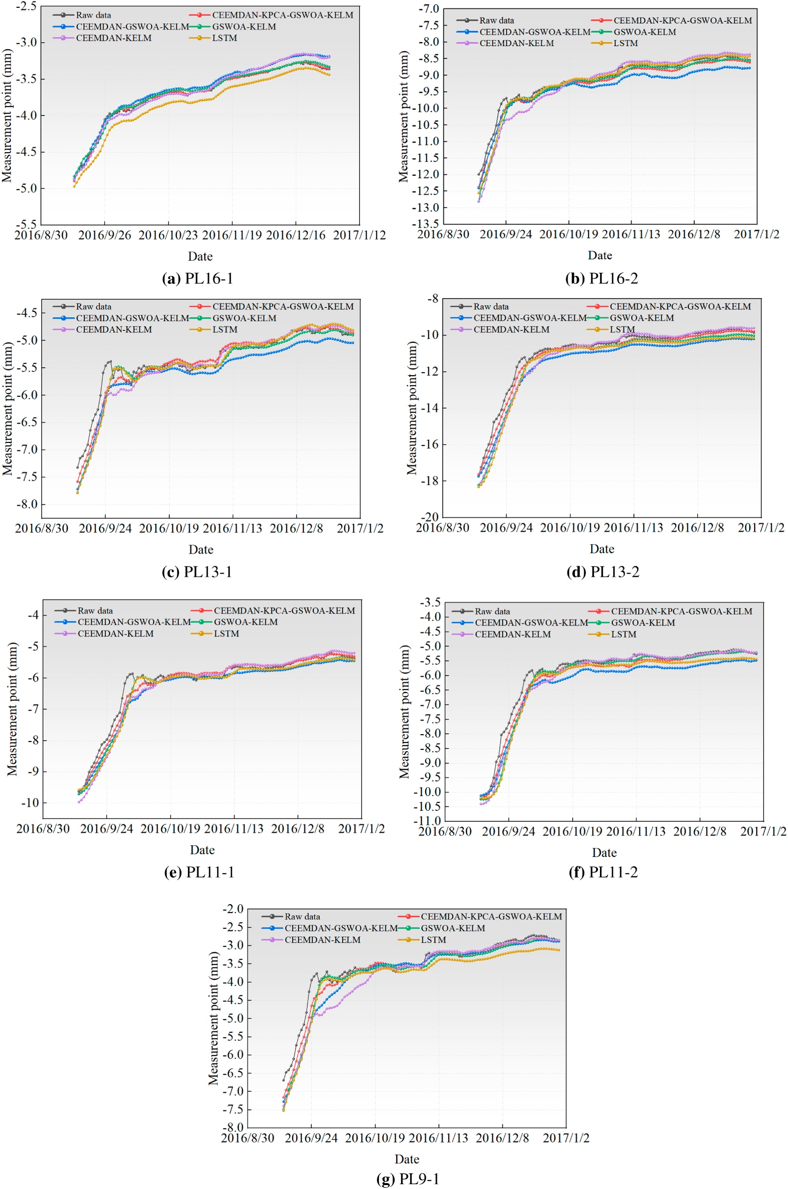
Figure A1: Comparison of prediction results for remaining measurement points in zone 1. (a) PL16-1; (b) PL16-2; (c) PL13-1; (d) PL13-2; (e) PL11-1; (f) PL11-2; (g) PL9-1.
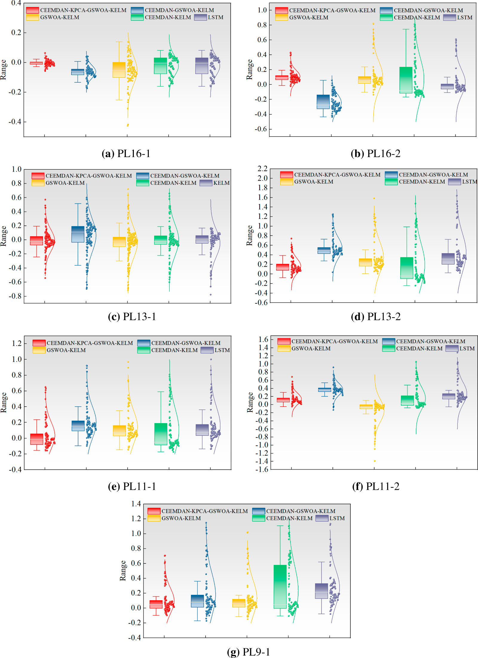
Figure A2: Box plot of residuals from the predictive model for the remaining measurement points in Zone 1. (a) PL16-1; (b) PL16-2; (c) PL13-1; (d) PL13-2; (e) PL11-1; (f) PL11-2; (g) PL9-1.
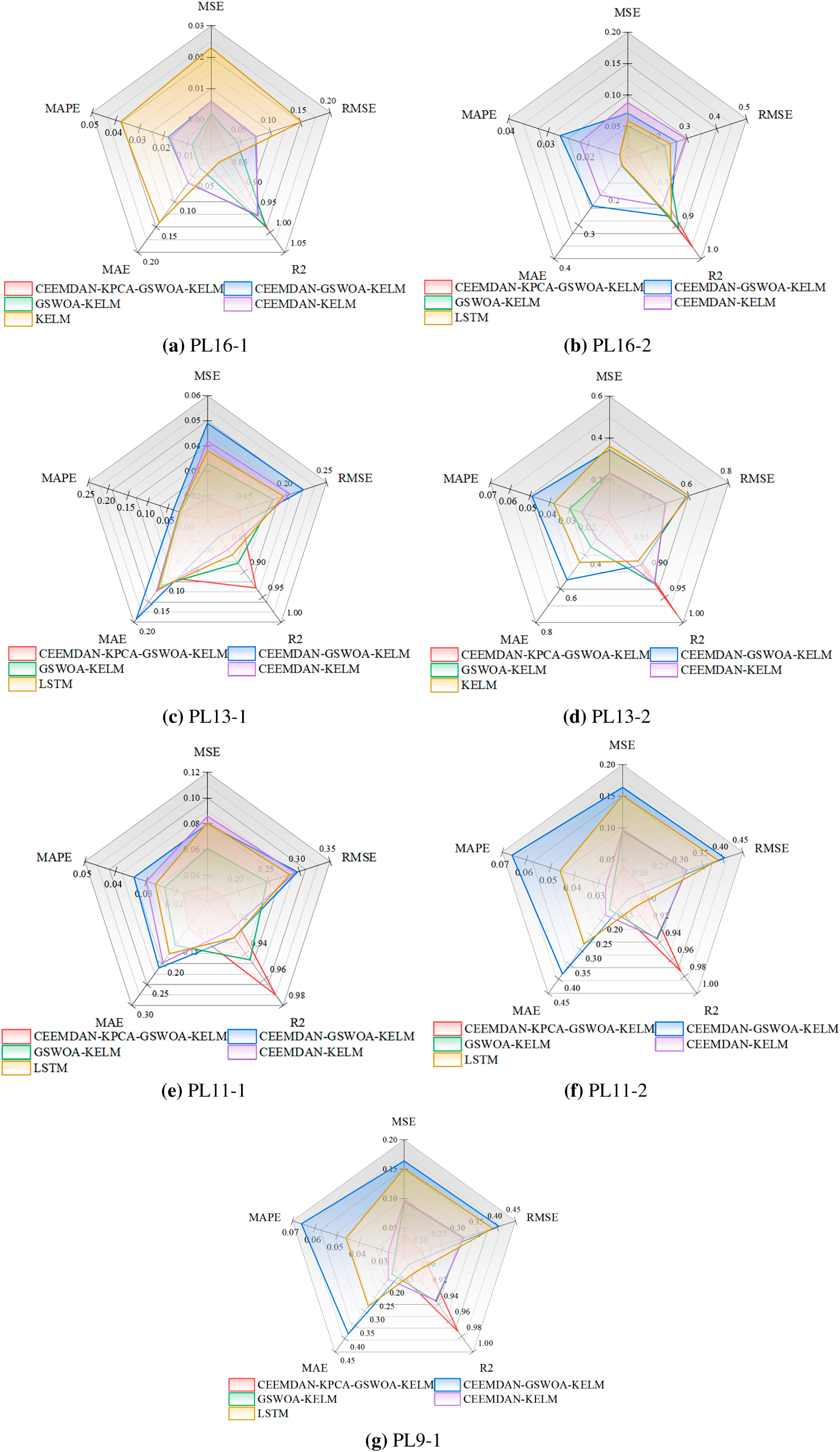
Figure A3: Model evaluation metrics for the remaining measurement points in Zone 1. (a) PL16-1; (b) PL16-2; (c) PL13-1; (d) PL13-2; (e) PL11-1; (f) PL11-2; (g) PL9-1.
References
1. Yuan D, Wei B, Xie B, Zhong Z. Modified dam deformation monitoring model considering periodic component contained in residual sequence. Struct Control Health Monit. 2020;27(12):e2633. doi:10.1002/stc.2633. [Google Scholar] [CrossRef]
2. Yuan R, Su C, Cao E, Hu S, Zhang H. Exploration of multi-scale reconstruction framework in dam deformation prediction. Appl Sci. 2021;11(16):7334. doi:10.3390/app11167334. [Google Scholar] [CrossRef]
3. Ren Q, Li M, Song L, Liu H. An optimized combination prediction model for concrete dam deformation considering quantitative evaluation and hysteresis correction. Adv Eng Inform. 2020;46(3):101154. doi:10.1016/j.aei.2020.101154. [Google Scholar] [CrossRef]
4. Li M, Wang J. An empirical comparison of multiple linear regression and artificial neural network for concrete dam deformation modelling. Math Probl Eng. 2019;2019(1):7620948. doi:10.1155/2019/7620948. [Google Scholar] [CrossRef]
5. Sortis DA, Paoliani P. Statistical analysis and structural identification in concrete dam monitoring. Eng Struct. 2007;29(1):110–20. doi:10.1016/j.engstruct.2006.04.022. [Google Scholar] [CrossRef]
6. Cai S, Gao H, Zhang J, Peng M. A self-attention-LSTM method for dam deformation prediction based on CEEMDAN optimization. Appl Soft Comput. 2024;159:111615. doi:10.1016/j.asoc.2024.111615. [Google Scholar] [CrossRef]
7. Li M, Bao T, Yang J, Ren J. Fractal geometric monitoring model of dam deformation based on improved grey model. Hydro Sci Eng. 2016;4:104–10. (In Chinese). doi:10.16198/j.cnki.1009-640X.2016.04.015. [Google Scholar] [CrossRef]
8. Xing Y, Chen Y, Huang S, Wang P, Xiang Y. Research on dam deformation prediction model based on optimized SVM. Processes. 2022;10(9):1842. doi:10.3390/pr10091842. [Google Scholar] [CrossRef]
9. Li M, Pan J, Liu Y, Wang Y, Zhang W, Wang J. Dam deformation forecasting using SVM-DEGWO algorithm based on phase space reconstruction. PLoS One. 2022;17(6):e0267434. doi:10.1371/journal.pone.0267434. [Google Scholar] [PubMed] [CrossRef]
10. Dai B, Gu C, Zhao E, Qin X. Statistical model optimized random forest regression model for concrete dam deformation monitoring. Struct Control Health Monit. 2018;25(6):e2170. doi:10.1002/stc.2170. [Google Scholar] [CrossRef]
11. Zhang S, Zheng DJ, Chen ZY. Dam deformation prediction model based on improved PSO-RF algorithm. Adv Sci Technol Water Resour. 2022;42(6):39–44. (In Chinese). doi:10.3880/j.issn.1006-7647.2022.06.007. [Google Scholar] [CrossRef]
12. Kose E, Tasci L. Geodetic deformation forecasting based on multi-variable grey prediction model and regression model. Grey Syst Theory Appl. 2019;9(4):464–71. doi:10.1108/gs-04-2019-0007. [Google Scholar] [CrossRef]
13. Wang X, Yang K, Shen C. Study on MPGA-BP of gravity dam deformation prediction. Math Probl Eng. 2017;2017(1):2586107. doi:10.1155/2017/2586107. [Google Scholar] [CrossRef]
14. Cheng J, Xiong Y. Application of extreme learning machine combination model for dam displacement prediction. Procedia Comput Sci. 2017;107(7):373–8. doi:10.1016/j.procs.2017.03.120. [Google Scholar] [CrossRef]
15. Su H, Li X, Yang B, Wen Z. Wavelet support vector machine-based prediction model of dam deformation. Mech Syst Signal Process. 2018;110:412–27. doi:10.1016/j.ymssp.2018.03.022. [Google Scholar] [CrossRef]
16. Su H, Chen Z, Wen Z. Performance improvement method of support vector machine-based model monitoring dam safety. Struct Control Health Monit. 2016;23(2):252–66. doi:10.1002/stc.1767. [Google Scholar] [CrossRef]
17. Cheng L, Zheng D. Two online dam safety monitoring models based on the process of extracting environmental effect. Adv Eng Softw. 2013;57:48–56. doi:10.1016/j.advengsoft.2012.11.015. [Google Scholar] [CrossRef]
18. Cao E, Bao T, Gu C, Li H, Liu Y, Hu S. A novel hybrid decomposition—ensemble prediction model for dam deformation. Appl Sci. 2020;10(16):5700. doi:10.3390/app10165700. [Google Scholar] [CrossRef]
19. Zhang Y, Zhang W, Li Y, Wen L, Sun X. A multi-output prediction model for the high arch dam displacement utilizing the VMD-DTW partitioning technique and long-term temperature. Expert Syst Appl. 2025;267(119):126135. doi:10.1016/j.eswa.2024.126135. [Google Scholar] [CrossRef]
20. Ou B, Zhang C, Xu B, Fu S, Liu Z, Wang K. Innovative approach to dam deformation analysis: integration of VMD, fractal theory, and WOA-DELM. Struct Control Health Monit. 2024;2024(1):1710019. doi:10.1155/2024/1710019. [Google Scholar] [CrossRef]
21. Sun X, Lu T, Hu S, Wang H, Wang Z, He X, et al. A new algorithm for predicting dam deformation using grey wolf-optimized variational mode long short-term neural network. Remote Sens. 2024;16(21):3978. doi:10.3390/rs16213978. [Google Scholar] [CrossRef]
22. Liu WQ, Chen B, Ge PM, Zhang XL. Deformation prediction model of a high arch dam based on clustering and MO-LSSVR. Adv Sci Technol Water Resour. 2023;43(2):102–8. (In Chinese). doi:10.3880/j.issn.10067647.2023.02.016. [Google Scholar] [CrossRef]
23. Li M, Pan J, Liu Y, Liu H, Wang J, Zhao Z. A deformation prediction model of high arch dams in the initial operation period based on PSR-SVM-IGWO. Math Probl Eng. 2021;2021:8487997. doi:10.1155/2021/8487997. [Google Scholar] [CrossRef]
24. Long J, Zuo SL, Xu L, Qi YN, Su HZ. Dam deformation prediction model based on impact factors screening and GWO-KELM. China Rural Water Hydrop. 2024;8:194–9. (In Chinese). doi:10.12396/znsd.231922. [Google Scholar] [CrossRef]
25. Lu Z, Ding Y, Li D. Coupling VMD and MSSA denoising for dam deformation prediction. Structures. 2023;58(1):105503. doi:10.1016/j.istruc.2023.105503. [Google Scholar] [CrossRef]
26. Bian K, Wu Z. Data-based model with EMD and a new model selection criterion for dam health monitoring. Eng Struct. 2022;260:114171. doi:10.1016/j.engstruct.2022.114171. [Google Scholar] [CrossRef]
27. Shi JC, Yue CF, Zhu MY, Pi LL. Improved wavelet thresholding combined with optimized BiLSTM for dam deformation prediction. J Hydroelectr Eng. 2024;43(7):97–108. (In Chinese). doi:10.11660/slfdxb.20240709. [Google Scholar] [CrossRef]
28. MacQueen J. Some methods for classification and analysis of multivariate observations. In: 5th Berkeley Symposium on Mathematical Statistics and Probability. Berkeley, CA, USA: University of California Press; 1967. p. 281–97. [Google Scholar]
29. Li B, Liang W, Yang S, Zhang L. Automatic identification of modal parameters for high arch dams based on SSI incorporating SSA and K-means algorithm. Appl Soft Comput. 2023;138:110201. doi:10.1016/j.asoc.2023.110201. [Google Scholar] [CrossRef]
30. Li H, Zeng S, Liu B, Wang G, Tang Y, Wang W, et al. Automatic operational modal analysis for high arch dams using enhanced SSI-COV with adaptive MVMD and improved FCM clustering algorithm. Adv Eng Inform. 2026;71:104257. doi:10.1016/j.aei.2025.104257. [Google Scholar] [CrossRef]
31. Torres ME, Colominas MA, Schlotthauer G, Flandrin P. A complete ensemble empirical mode decomposition with adaptive noise. In: 2011 IEEE International Conference on Acoustics, Speech and Signal Processing (ICASSP); 2011 May 22–27; Prague, Czech Republic. p. 4144–7. doi:10.1109/ICASSP.2011.5947265. [Google Scholar] [CrossRef]
32. Mirjalili S, Lewis A. The whale optimization algorithm. Adv Eng Softw. 2016;95:51–67. doi:10.1016/j.advengsoft.2016.01.008. [Google Scholar] [CrossRef]
33. Liu M, Feng Y, Yang S, Su H. Dam deformation prediction considering the seasonal fluctuations using ensemble learning algorithm. Buildings. 2024;14(7):2163. doi:10.3390/buildings14072163. [Google Scholar] [CrossRef]
34. Wang C, Qi S, Wang T, Xiong Z, Wang Q, Liu Y, et al. GSWOA-KELM model for predicting slope stability and its engineering application. Nat Hazards. 2025;121(11):12721–39. doi:10.1007/s11069-025-07260-w. [Google Scholar] [CrossRef]
35. Wang L, Wang J, Tong D, Wang X. A novel long short-term memory Seq2Seq model with chaos-based optimization and attention mechanism for enhanced dam deformation prediction. Buildings. 2024;14(11):3675. doi:10.3390/buildings14113675. [Google Scholar] [CrossRef]
36. Kang F, Liu X, Li J. Temperature effect modeling in structural health monitoring of concrete dams using kernel extreme learning machines. Struct Health Monit. 2020;19(4):987–1002. doi:10.1177/1475921719872939. [Google Scholar] [CrossRef]
37. Li M, Shen Y, Ren Q, Li H. A new distributed time series evolution prediction model for dam deformation based on constituent elements. Adv Eng Inform. 2019;39(3):41–52. doi:10.1016/j.aei.2018.11.006. [Google Scholar] [CrossRef]
38. Jin Y, Liu X, Huang X. CEEMDAN-FTEA-GCN-Transformer: a transformer-based model for dam deformation prediction with frequency-spatial feature integration. Results Eng. 2025;28:108154. doi:10.1016/j.rineng.2025.108154. [Google Scholar] [CrossRef]
39. Yuan D, Gu C, Wei B, Qin X, Xu W. A high-performance displacement prediction model of concrete dams integrating signal processing and multiple machine learning techniques. Appl Math Model. 2022;112:436–51. doi:10.1016/j.apm.2022.07.032. [Google Scholar] [CrossRef]
40. Chen X, Chen Z, Hu S, Gu C, Guo J, Qin X. A feature decomposition-based deep transfer learning framework for concrete dam deformation prediction with observational insufficiency. Adv Eng Inform. 2023;58:102175. doi:10.1016/j.aei.2023.102175. [Google Scholar] [CrossRef]
41. Zhou B, Wang Z, Fu S, Chen D, Yin T, Gao L, et al. Dam deformation prediction model based on multi-scale adaptive kernel ensemble. Water. 2024;16(13):1766. doi:10.3390/w16131766. [Google Scholar] [CrossRef]
42. Wang Z, Fu S, Chen D, Han Z, Wang W, Ou B. A multipoint spatiotemporal prediction model for concrete dams integrating hybrid clustering and adaptive decomposition-optimization mechanisms. Struct Control Health Monit. 2025;2025(1):4005246. doi:10.1155/stc/4005246. [Google Scholar] [CrossRef]
Cite This Article
 Copyright © 2026 The Author(s). Published by Tech Science Press.
This work is licensed under a Creative Commons Attribution 4.0 International License , which permits unrestricted use, distribution, and reproduction in any medium, provided the original work is properly cited.
 Downloads
 Citation Tools