Learning-Based Prediction of Soft-Tissue Motion for Latency Compensation in Teleoperation

1  Introduction

Robotic teleoperation in medical settings such as ultrasound imaging, minimally invasive endoscopy, and tissue sampling often requires stable and precise target tracking over dynamically moving soft tissue [1–5]. Inevitably, end-to-end latencies across the perception–computation–execution chain induce response lag and amplitude distortion relative to the true target, with pronounced peak attenuation and phase lag around trajectory kinks or high-acceleration segments, thereby compromising safety margins and positioning accuracy [6–8]. A proven approach is to incorporate motion prediction: using past observations to forecast near-future target states and feeding these estimates forward to counteract the deleterious effect of delay on closed-loop performance [9–11]. On our teleoperation platform, system analysis and empirical observations show that camera acquisition, temporal reconstruction, inverse kinematics, and actuation jointly determine an effective collaboration. When the prediction horizon is aligned to this lead the system can suppress biased tracking and improve performance at kinks without altering hardware.

Research on soft-tissue motion prediction and tracking spans both model-driven and data-driven lines. Tuna et al. [12] proposed two least-squares-based predictors that generate future position estimates via adaptive filters: one assumes a linear system relationship among samples within the prediction window, while the other parameterizes each point independently over the horizon, highlighting the feasibility—and limitations—of online recursion and locality assumptions in surgical contexts. To tackle complex intraoperative deformations, poor imaging conditions, specular reflections, and other dynamics, Yang et al. [13] devised a 3D tracking scheme composed of two independent recursive processes: inter-frame, they represent the target region in joint spatial–color space and define a probabilistic similarity measure to derive a mean-shift iterative localization in the new image; intra-frame, they fit a thin-plate spline surface around the target and solve for optimal model parameters using an efficient second-order minimization procedure, coupling appearance and geometry to enhance robustness. While such approaches leverage structural priors and stable optimization, they still require careful parameter tuning and compute–accuracy trade-offs under rapid changes and strong noise.

For periodic and quasi-periodic physiological motion, Yang et al. [14] modeled cardiac motion with a double time-varying Fourier series, estimating frequency parameters and Fourier coefficients via dual Kalman filters to sidestep limitations from model linearization; the method independently tracks instantaneous respiratory and cardiac frequencies and performs well on both synthetic and real data. Building on this, Yang et al. [15] combined the online measurement of instantaneous frequencies with observed 3D trajectories of points of interest, exploiting directional differences between respiratory and cardiac motions and extracting an optimal one-dimensional principal component signal to estimate instantaneous frequencies robustly. These studies underscore the interpretability and effectiveness of spectral/state-estimation models for quasi-periodic motion, yet their adaptability to abrupt disturbances, occlusions, and local transients remains bound by prior assumptions.

On the data-driven side, deep sequence models have demonstrated stronger nonlinear fitting capacity and end-to-end learning potential. Zhang et al. used long short-term memory (LSTM) networks for offline modeling and prediction of heartbeat signals, confirming neural networks’ accuracy and robustness for time-series forecasting; by adding auxiliary spatial points, they further improved prediction accuracy, indicating the benefits of multi-source observations [16]. Nevertheless, many studies still treat the prediction horizon as a heuristic hyperparameter and lack a unified framework that aggregates latencies from perception, inference, inverse kinematics, and execution to derive an optimal lead. This misalignment between the “learned future” and the “past to be canceled,” together with the absence of a common evaluation protocol across models and data domains, hinders fair comparison and practical integration [17–19].

Against this backdrop, introducing a Temporal Convolutional Network (TCN) is well-motivated. Built on causal and dilated convolutions, TCNs achieve controllable large receptive fields without violating temporal causality; their convolutional and parallel nature typically yields more stable inference latency and higher throughput—well-suited to the fixed-rate, low-jitter demands of real-time teleoperation. Convolutional kernels are inherently sensitive to local shape changes and high-frequency components, aiding responsiveness and gradient stability near kinks and rapid transients. Moreover, TCNs facilitate multi-step forecasting via a single forward pass with consistent temporal alignment, making it straightforward to interface with an end-to-end latency budget [20,21]. In this sense, TCNs complement LSTMs: the former offers potential advantages for real-time constraints and local transient capture, while the latter is well-established for mixed long-/short-term dependencies. Evaluating both—alongside a lightweight AR baseline—under a unified protocol on in vivo and phantom domains not only clarifies each model’s applicability boundaries but also supplies robust options for latency–horizon alignment [22].

In summary, we target the closed-loop need of “soft-tissue motion prediction → latency alignment → motion compensation.” We decompose end-to-end delay into sensing, inference, inverse kinematics, and actuation, normalize by the sampling period, and obtain an optimal prediction horizon that aligns the forecasted state with the actual control application time. Across in vivo and phantom datasets, we systematically evaluate AR, LSTM, and TCN under consistent splits and metrics, with particular attention to error mechanisms and compensation effectiveness around kinks and high-acceleration segments. Our results show that an aligned prediction-and-control integration substantially reduces both steady-state and peak errors, while demonstrating the feasibility and potential advantages of TCNs in real-time teleoperation, thereby providing methodological and engineering support for deploying predictive compensation in practical systems.

2  Methodology

The physiological activities of the human body are generally cyclical, such as breathing and heartbeat. The movements of body parts affected by such physiological activities also have their own regularity. The trajectory of the human body’s points of interest affected by physiological activities is actually a set of time series data, representing the changes along the time axis represented by coordinates in three directions. Establishing its motion model is essentially completing a time series modeling task. The time series modeling task can be expressed as follows: Assume that there is an input time series (x0,x1,…,xT), and it is necessary to predict the corresponding output (y0,y1,…,yT) based on this sequence. Then the sequence modeling task is to establish the following mapping relationship based on the data, as shown in Eq. (1):

y^0,…,y^T=f(x0,…,xT)(1)

This study selected three different models to model heartbeat trajectory data and perform predictions to observe the feasibility of the network model and the accuracy of the predictions. These three models are autoregressive (AR), LSTM, and TCN.

2.1 Autoregressive Method

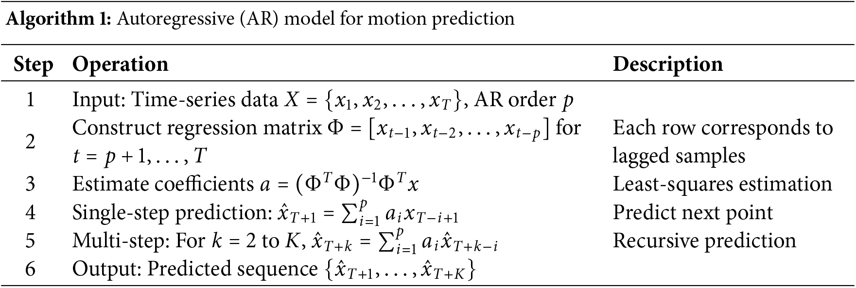
Autoregression [23,24] is a method for predicting future data using historical data. Specifically, it uses a regression equation to predict the time series of a variable based on its dependency on the time series of the same variable projected a certain amount of time into the past.

Time series data Xt can usually be represented by the superposition of weighted historical data and random disturbances, as shown in Eq. (2):

Xt=a1Xt−1+a2Xt−2+⋯+apXt−p+εt=∑i=1paiXt−i+εt(2)

where a=(a1,a2,…,ap) is the autoregressive coefficient in the model, and ε represents the random disturbance.

Forecasting using an autoregressive model requires only sliding a window based on historical experimental data and calculating the weighted sum of the contributions of each historical moment within the window to the next moment within the sliding window. Assume that the sequence data within a sliding window of length m is (t1,p1),(t2,p2),…,(tm,pm). The parameterization method can be shown in Eq. (3):

a=n∑i=1ntipi−∑i=1nti∑i=1npin∑i=1nti2−(∑i=1nti)2ε=1n∑i=1npi−an∑i=1nti(3)

The AR model predicts future states as weighted combinations of past observations, with coefficients estimated by least squares. The computational steps are summarized in Algorithm 1.

2.2 LSTM Network Training

The LSTM model [25] has relatively few parameters to choose from. The basic network structure is shown in Fig. 1.

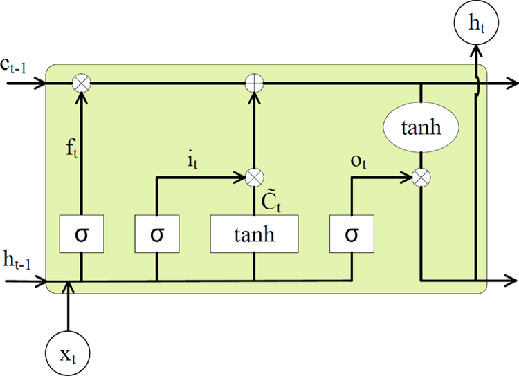
Figure 1: LSTM network structure

After establishing the model structure, the only parameters that need to be determined are the number of hidden neurons (num_hidden) and the number of hidden layers (levels). Then, based on the data format, the network’s input and output dimensions are determined.

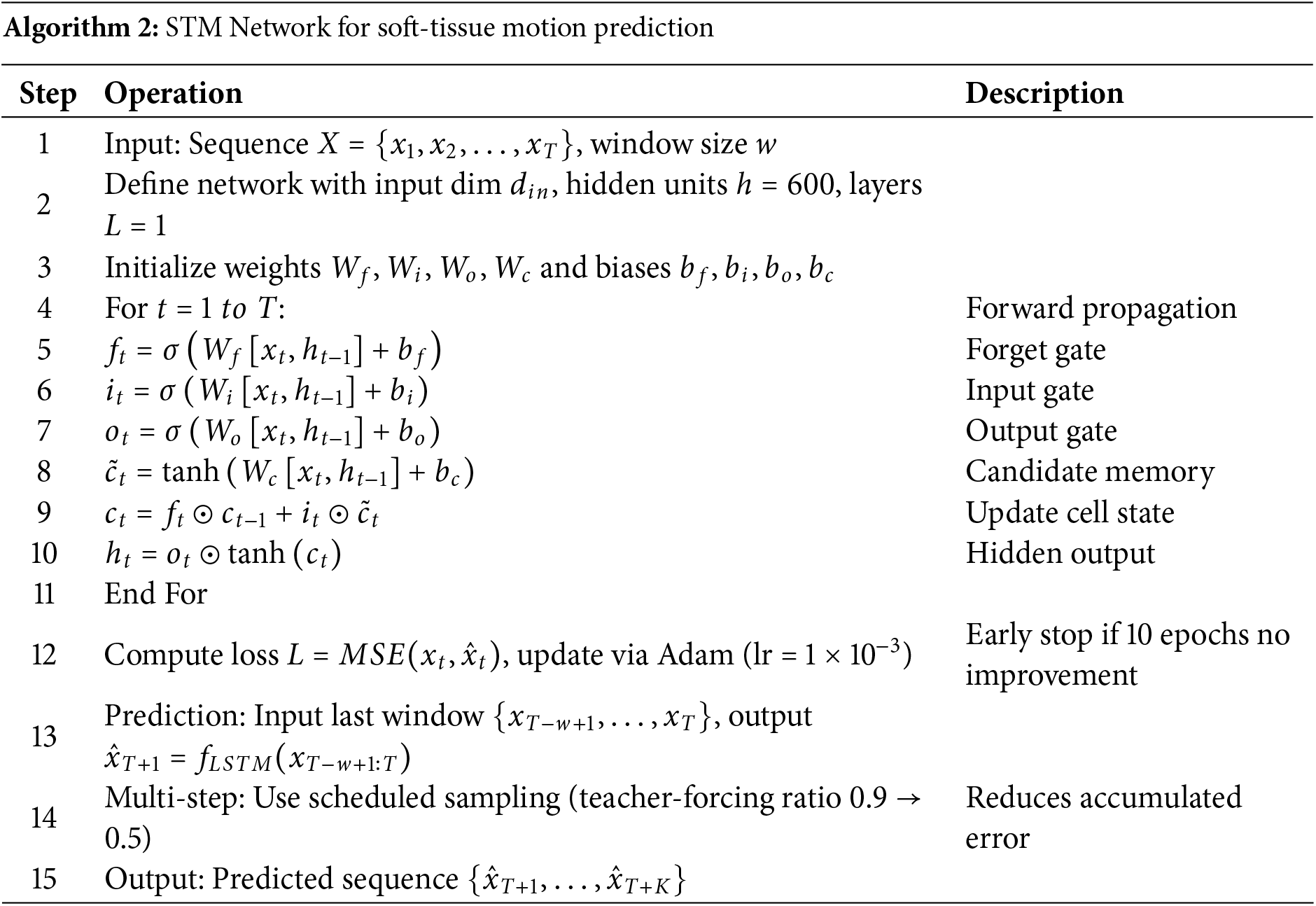
In this study, the number of hidden neurons and the number of hidden layers were set to 600 and 1, respectively, which achieved good prediction results. The LSTM network training data set does not need to be divided or integrated into other formats. Simply extract the input data and output data from the original data and convert them into tensors. The detailed training and prediction procedure is outlined in Algorithm 2.

2.3 TCN Network Training

The network structure of TCN [26] is shown in Fig. 2. The more important parameters in the network model are the convolution kernel size, the number of convolution hidden layers, the dilation factor, the batch size, and the window size (hereinafter referred to as w_s).

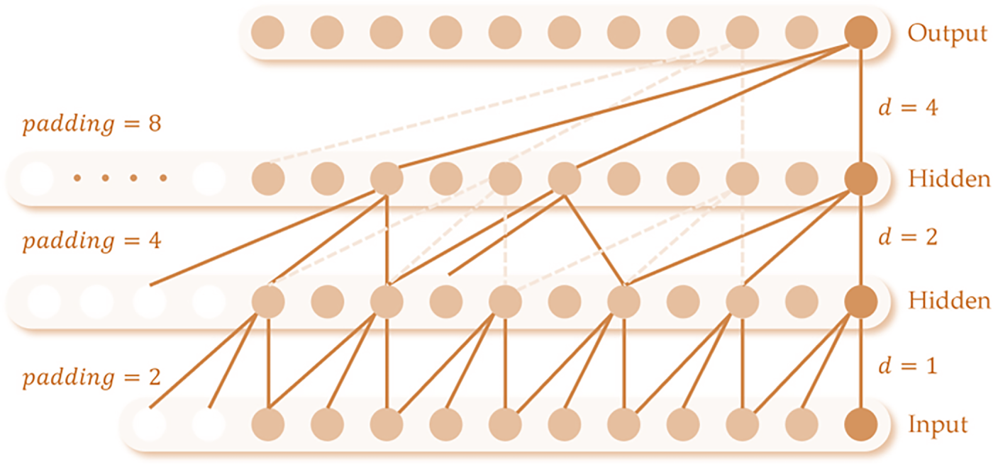
Figure 2: TCN network structure

In this study, the TCN parameters were set to kernel_size=3, levels=3 and batch_size=128. The convolution kernel size, the number of hidden layers, and the dilation factor collectively determine the range of historical information available for current predictions: larger parameters increase the reference range. In this network, the dilation factors for the hidden layers and the final output layer are 20, 21, 22, and 23.

The window size w_s is a crucial parameter when processing datasets to generate training and test sets. It determines the size of the input data fed into the model. Since two datasets (in vivo and Phantom) are used, the specific characteristics of each dataset vary, particularly in terms of periodicity and motion regularity. The POI trajectory data in the in vivo dataset considers both heartbeat and respiration components, while the Phantom dataset only considers heartbeat components. Since the periods of the two datasets are inconsistent, different window sizes are used for each dataset to ensure that the model learns the full cycle and the periodic nature of motion during training.

In subsequent experiments, the window size w_s was 50 for the in vivo dataset and 35 for the Phantom dataset. Using the determined parameter w_s as the sliding window size, after each sliding window, all data within the window are arranged in their original order as a new set of inputs, and the next data outside the window is used as the output corresponding to that set of inputs. The model input data scale of the training set is (600−ws,3,w_s), which is (550,3,50) in the in vivo dataset and (565,3,35) in the Phantom dataset. Its main configuration and inference process are presented in Algorithm 3.

2.4 Loss Functions

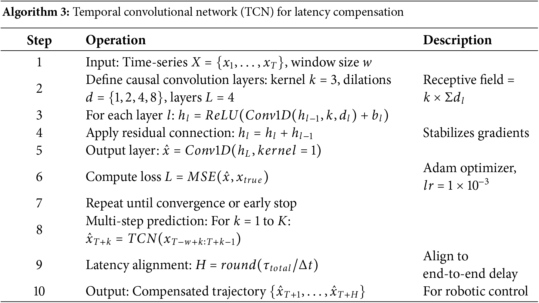
During the training process, the loss function is calculated using the mean square error (MSE) and is defined as the square of the Euclidean distance between the actual coordinates of the interest point and the predicted coordinates. MSE penalizes large errors, meeting the safety requirements of ‘avoiding significant deviations’ in medical scenarios. It is shown in Eq. (4):

loss=1n∑i=1n(pointpre−pointact)2(4)

Among them, pointpre represents the predicted coordinates of the interest point; pointact represents the true value of the coordinates of the interest point.

For multi-step prediction, an iterative multi-step learning strategy was employed. During training, each model first predicts one-step ahead pointpre, and the resulting prediction is then recursively fed into the network to generate subsequent steps. The total multi-step loss is computed as the average of the MSE values over the entire prediction horizon np, as shown in Eq. (5):

lossmulti=1np∑i=1np1n∑i=1n(pointpre−pointact)2(5)

3  Experimental Setting

This research focuses on implementing motion compensation when a teleoperation platform tracks the motion of a point of interest. Therefore, a binocular camera is used as a motion signal collector, and the spatial position of the tracking target is analyzed based on the motion image. In subsequent simulations, a data set is sampled at a fixed frequency to simulate the binocular camera’s signal acquisition and positioning operations. Based on the established teleoperation platform, only the robotic arm is controlled to complete motion compensation simulations. The simulation flow is shown in Fig. 3, where a, b, c, and d represent the key steps in motion compensation teleoperation.

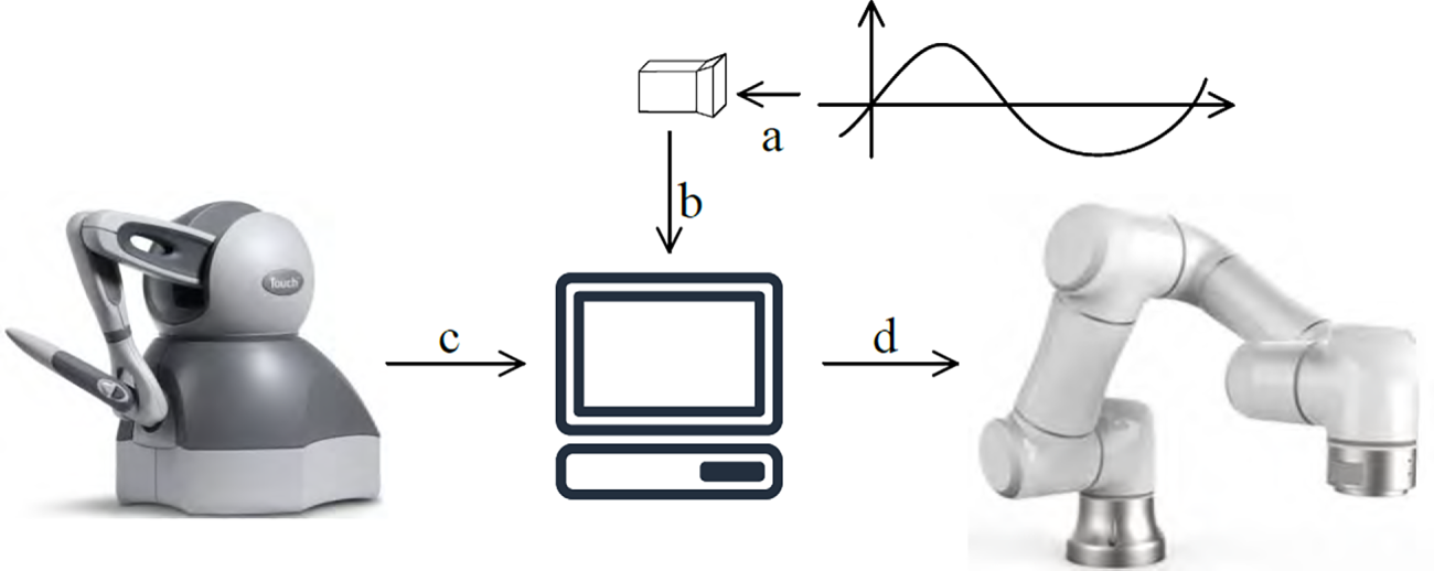
Figure 3: Schematic diagram of the simulation experiment platform

In process (a), a camera observes the motion of a point of interest in the workspace, spatially localizes the point of interest, and obtains its three-dimensional coordinates. In process (b), the camera transmits the coordinates of the point of interest to the robotic arm host computer as part of the control command.

In process (c), the proximal (control handle) host computer issues a query command to the handle, querying the current position of the handle end in the handle base coordinate system. The handle reads the end state Btouchx0 and sends it to the distal (robotic arm) host computer as another part of the control command.

In process (d), the target poses information collected in processes (b) and (c) is combined to perform an inverse kinematic solution, obtaining the states Q=(q1,q2,q3,q4,q5,q6) of each joint of the robotic arm. q1,q2,q3,q4,q5,q6 represent the six joint rotation angles (in radians) of the Elite EC63 six-axis robotic arm. These are then issued as control commands to the robotic arm, causing it to move to the target pose.

The target pose information in process d comprises both the target pose information for teleoperation, and the target pose information for motion tracking of the point of interest. The former completes the teleoperation task, and the latter realizes the motion tracking effect and compensates for the movement of the point of interest.

The hardware and software environment used in the simulation experiments in this study are shown in Table 1.

3.1 Experimental Dataset

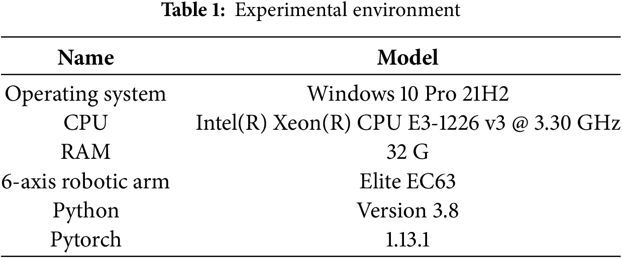
The robotic arm’s motion instructions are still based on quasi-periodic physiological motion. According to studies such as [15,27,28], physiological motion affecting relevant points on the heart surface can be decomposed into heartbeat motion and respiratory motion. Both are periodic, and their trajectory functions can be decomposed into sinusoidal motions of varying orders. In the experiment, heartbeat and respiratory motions were simulated using sinusoidal function signals of varying periods and then verified using a real-world dataset.

3.1.1 Simulated Signal Dataset

In the simulated signal, the heartbeat component of the motion of the point of interest has a period of 4 s and an amplitude of 1 mm. The respiratory component has a period of 0.875 s and an amplitude of 1 mm. These values align with the normal human physiological range: a heart rate of 60–100 beats per minute corresponds to a cycle of 0.6–1 s. The respiratory component is the primary interfering factor in the heartbeat component. Other interference (noise) is not considered. This is because during training, the neural network learns the main patterns in the data; noise is not generally regular and is automatically filtered out. The motion trajectories of the simulated physiological motion components and the synthesized motion trajectory image are shown in Fig. 4.

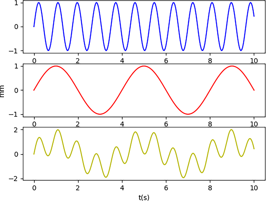
Figure 4: Simulated signal heartbeat component (blue), respiratory component (red), and synthetic motion (yellow)

3.1.2 Phantom Heart and Real Heart Datasets

This experiment used a real-world dataset based on the motion trajectories of points of interest on the surfaces of phantom and real hearts, captured by a da Vinci robot [29,30]. The dataset contains the 3D coordinates of 750 points, each corresponding to the position of the same point of interest in 750 frames of cardiac motion images sampled at a 25 Hz rate. These are continuous samples from one subject. Region of Interest (ROI) annotation was independently conducted by two senior surgeons, with an inter-annotator agreement of Kappa = 0.92.

The trajectories in the phantom dataset only account for heartbeat motion and do not include respiratory motion. The in vivo dataset, collected from the motion of points of interest on the surface of a real heart, considers both heartbeat and respiratory motion. Fig. 5 show the displacement changes of the points of interest trajectories in three different directions in the in vivo and phantom datasets.

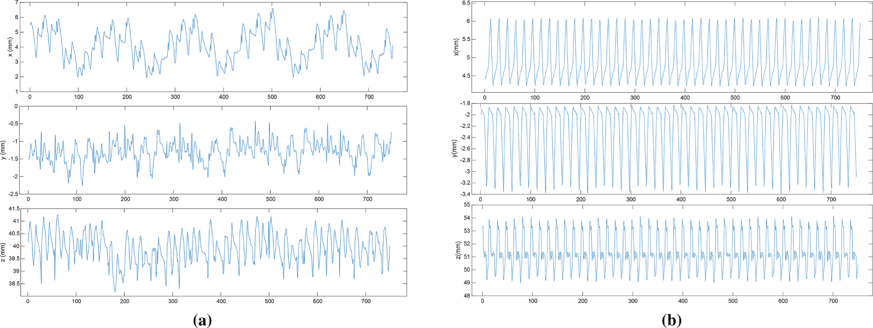
Figure 5: Displacement changes of interest point trajectory: (a) In vivo; (b) Phantom datasets

3.2 Model Prediction Performance Analysis

Before applying the model to motion compensation, we first conducted preliminary offline performance testing. In the experimental setup, we used the first 600 points from both the in vivo and Phantom datasets as the training set, and the subsequent 150 points in this section as the test set to test the model’s prediction performance. For autoregressive models, the prediction result is only the solution to the fitted local linear equation at a certain point in the future, so only single-step predictions are performed to observe performance. For both TCN and LSTM, both single-step and multi-step prediction performance tests were performed.

For single-step prediction, the model input is a ground-truth sequence of appropriate length. The output prediction result is compared with the next ground-truth data in the input sequence to obtain the trajectory tracking performance and error of the single-step prediction.

To minimize the impact of different starting points on the prediction results and the randomness of model training, 20 models were trained on the same training set. For each model, single-step prediction was initiated using points 600 to 649 in the dataset as the prediction starting point, and prediction results for the next 100 steps were obtained. Based on the above experimental setup, prediction results for 20 × 50 × 100 points were obtained.

For all single-step prediction experiments, the root mean square error (RMSE) of the model’s single-step prediction was calculated as shown in Eq. (5). Compared to MSE, RMSE better reflects the overall performance of the model.

For all single-step prediction experiments, the Root Mean Square Error (RMSE unit: mm) was used as the primary evaluation metric to quantify the model’s prediction accuracy, as defined in Eq. (6). During network training, the Mean Square Error (MSE, unit: mm2) served as the loss function to penalize large deviations and ensure convergence stability. For evaluation and comparison, the RMSE obtained as the square root of MSE—was adopted because it shares the same physical unit as the predicted displacement, thereby offering more intuitive interpretation of spatial tracking accuracy.

RMSE=11000∑i=120∑j=150(Pk,i,jpre−Pk,i,jact)2(6)

where k represents the k-th point in the dataset for each prediction; i represents the i-th model used for prediction; and j represents the j-th prediction starting point when the same model is used for prediction.

In the model’s multi-step prediction experiments, the 600th point in the original dataset was still used as the first prediction point, and the prediction length was still 100 steps. Furthermore, to explore the model’s prediction performance at different prediction step sizes, prediction experiments were conducted with 5, 10, and 20 steps. Including the single-step prediction described above as a special case of multi-step prediction, a total of four multi-step prediction experiments with different step sizes were conducted.

3.3 Model Training and Statistical Analysis

All learning-based models were trained and evaluated under consistent data preprocessing and partitioning procedures to ensure comparability.

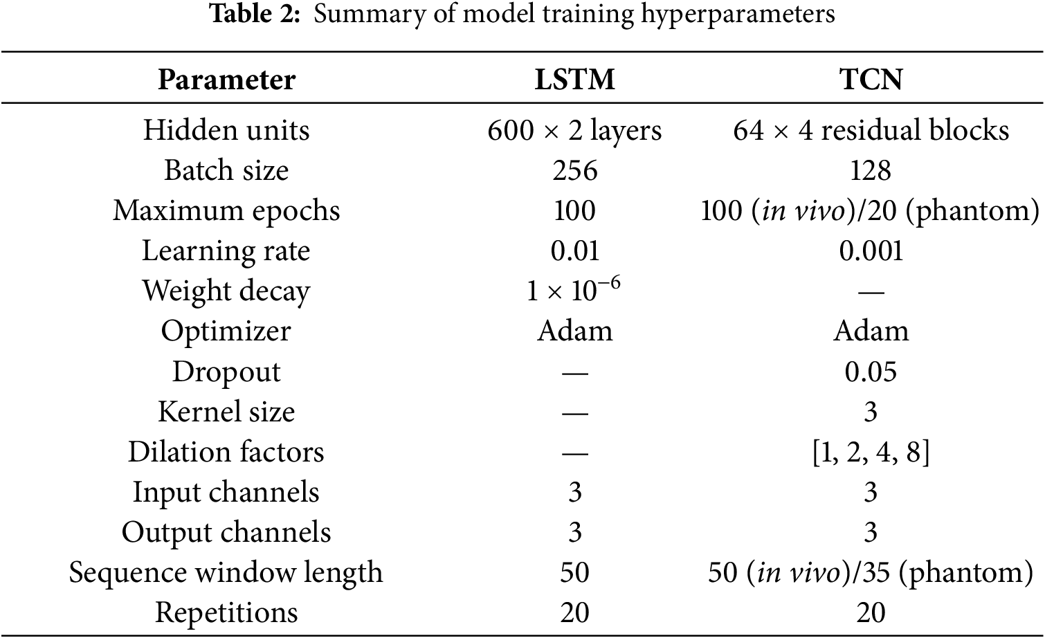
The LSTM network was composed of two stacked LSTM layers, each containing 600 hidden units. The batch size was set to 256, and the maximum number of training epochs was 100. The learning rate was 0.01, with a weight decay of 1 × 10−6. The network was trained using the Adam optimizer and the Mean Square Error (MSE) loss function. Training was terminated early if the validation loss did not improve for 10 consecutive epochs. The model was trained in both single-step and multi-step prediction modes, with one-step output and a prediction horizon of 50 frames. All predictions were subsequently transformed back to real coordinates (mm) using the inverse of the normalization parameters.

The TCN comprised four residual blocks with causal dilated convolutions (kernel size = 3; dilation factors = [1, 2, 4, 8]). Each block contained 64 hidden channels, and a dropout rate of 0.05 was applied for regularization. The input and output channel dimensions were both 3, corresponding to the 3D spatial motion components. Sequence window lengths were set to 50 for the in vivo dataset and 35 for the phantom dataset. The model was trained using the Adam optimizer (learning rate = 1 × 10−3) and the MSE loss function, retaining the model with the lowest validation loss.

Each model was trained 20 times under identical conditions to account for stochastic variations from random initialization. The mean ± standard deviation (SD) of the evaluation metrics was calculated to assess stability. A two-tailed Student’s t-test with a significance level of α = 0.05 was performed on the RMSE values to evaluate statistical significance. Differences were considered statistically significant when p < 0.05 and highly significant when p < 0.01. All reported results in Section 4 represent the mean ± SD across the 20 independent runs. These standardized training and analysis procedures ensure reproducibility and statistical rigor. Table 2 shows the detailed parameter settings for the above model.

4  Experimental Results and Analysis

4.1 Autoregressive Model Prediction Results

Fig. 6 demonstrates the performance of single-step predictions on a real dataset.

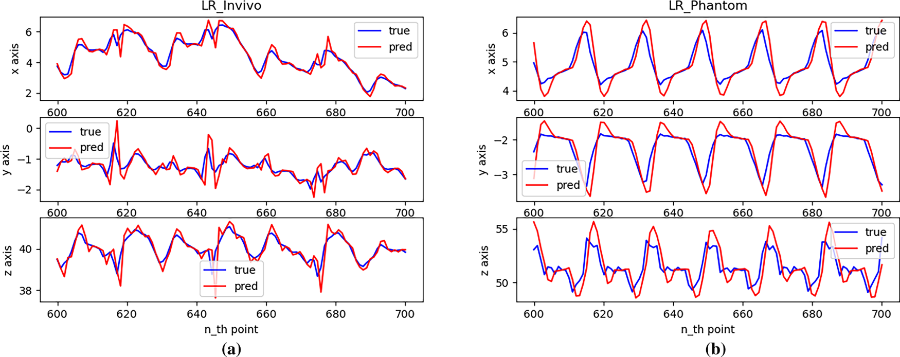
Figure 6: Single-step prediction effect with AR: (a) In vivo; (b) Phantom datasets

As can be seen from Fig. 6, due to the very small sliding window value of the autoregressive model, the model effectively predicts the next position when the trajectory changes smoothly across the entire test set. However, due to the principle of local linear fitting, the prediction results will have large errors at the inflection points of the trajectory.

Fig. 7 shows the single-step prediction error, MSE. As can be seen from Fig. 7, across the entire test set, the prediction error for the in vivo dataset ranges from 0 to 6.8 mm2, and for the Phantom dataset, from 0 to 8 mm2.

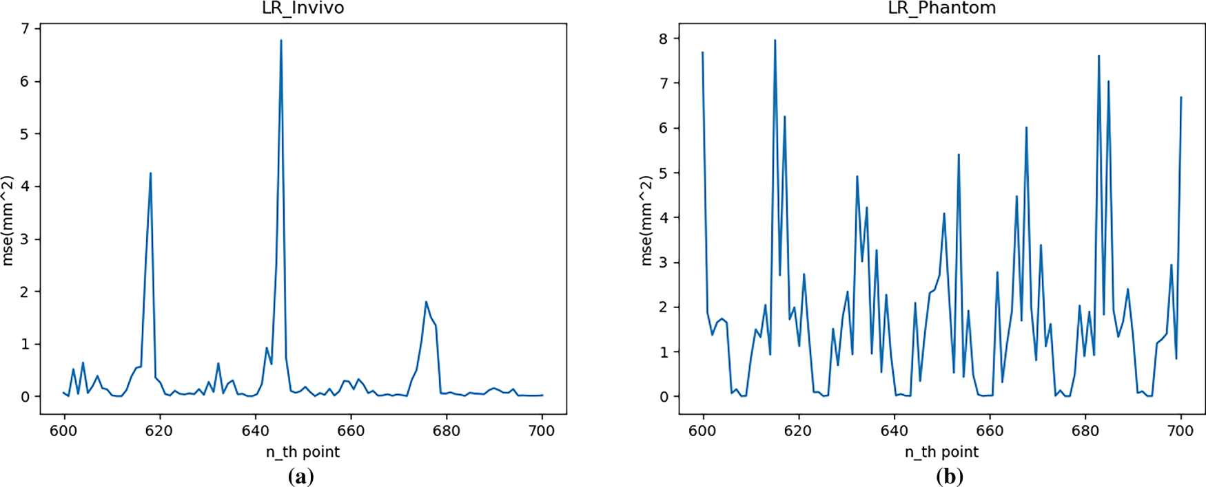
Figure 7: Single-step prediction error (MSE) with AR: (a) In vivo; (b) Phantom datasets

A simple autoregressive model performing only single-step predictions already performs poorly and is not suitable for practical use in fine motion prediction. However, it can serve as a baseline for comparison with other models to determine whether the model has effectively learned the sequence patterns in the dataset.

Statistically, the RMSE of the single-step predictions for the autoregressive model over a 100-step prediction range for the in vivo and Phantom datasets (to three decimal places) is 0.676 and 1.325 mm, respectively.

4.2 LSTM Model Prediction Results

The single-step prediction effect of the LSTM network is shown in Fig. 8, and the single-step prediction error is shown in Fig. 9.

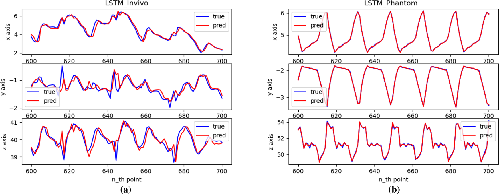
Figure 8: Single-step prediction effect with LSTM: (a) In vivo; (b) Phantom datasets

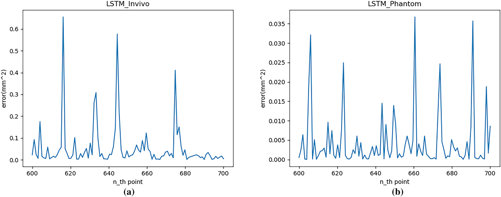
Figure 9: Single-step prediction error (MSE) with LSTM: (a) In vivo; (b) Phantom datasets

Fig. 8 shows that the LSTM network performs well for single-step predictions of time series data with objective patterns. Meanwhile, at inflection points in the trajectory, the prediction performance is relatively poor, with the prediction error being greater than when the trajectory is smoothed.

Fig. 9 shows that the LSTM network performs well for single-step predictions of regular time series data, confirming that datasets with stronger regularity exhibit better prediction performance. The MSE range for the in vivo dataset is 0 to 0.68 mm2, and for the Phantom dataset is 0 to 0.038 mm2. Furthermore, the moments of high error in this figure correspond precisely to inflection points in the trajectory. However, when the original trajectory smooths out, the model’s prediction error quickly returns to a lower level.

Furthermore, statistics show that for the in vivo and Phantom datasets, the LSTM model achieved a single-step RMSE of 0.222 and 0.111 mm, respectively, over a 100-step prediction range. It significantly reduces the prediction error compared to the autoregressive model. For the Phantom dataset, where the data is more regular, the RMSE is less than 9% of that of the autoregressive model.

The multi-step prediction errors of the LSTM network with different step sizes under two data sets are shown in Fig. 10.

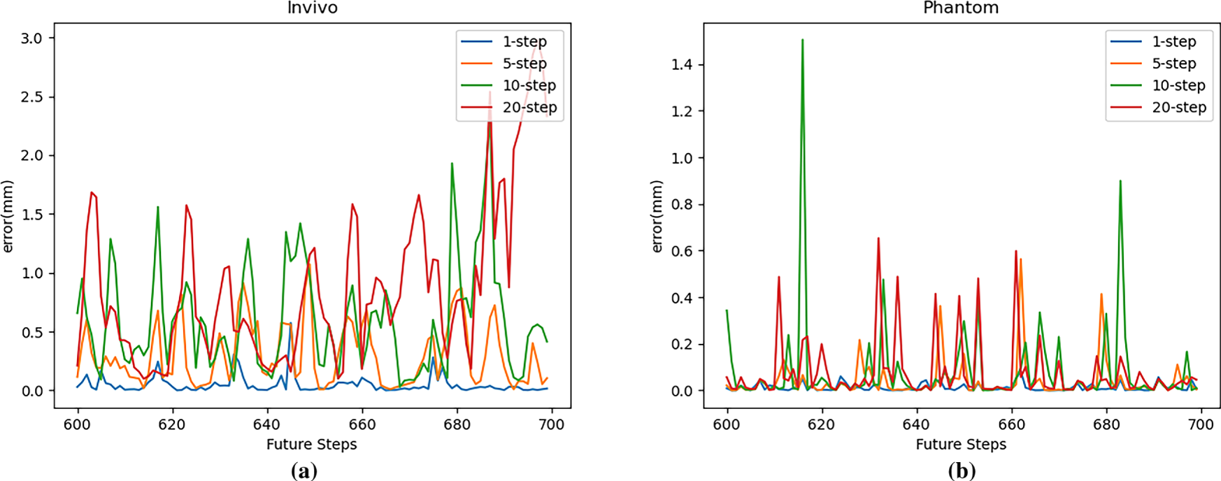
Figure 10: Multi-step prediction error (RMSE) with LSTM: (a) In vivo; (b) Phantom datasets

As can be seen from the figure, the model’s prediction error is smaller on the more regular Phantom dataset than on the in vivo dataset under the same experimental settings. For both the in vivo and Phantom datasets, the LSTM network’s multi-step prediction performance generally deteriorates with increasing prediction steps. The model achieves better prediction results with fewer prediction steps, which is also related to the model’s error accumulation during multi-step predictions.

4.3 TCN Model Prediction Results

Regarding the prediction performance of the model, we first conducted a single-step prediction test. The model prediction trajectory results are shown in Fig. 10; the average prediction error of each step is shown in Fig. 11.

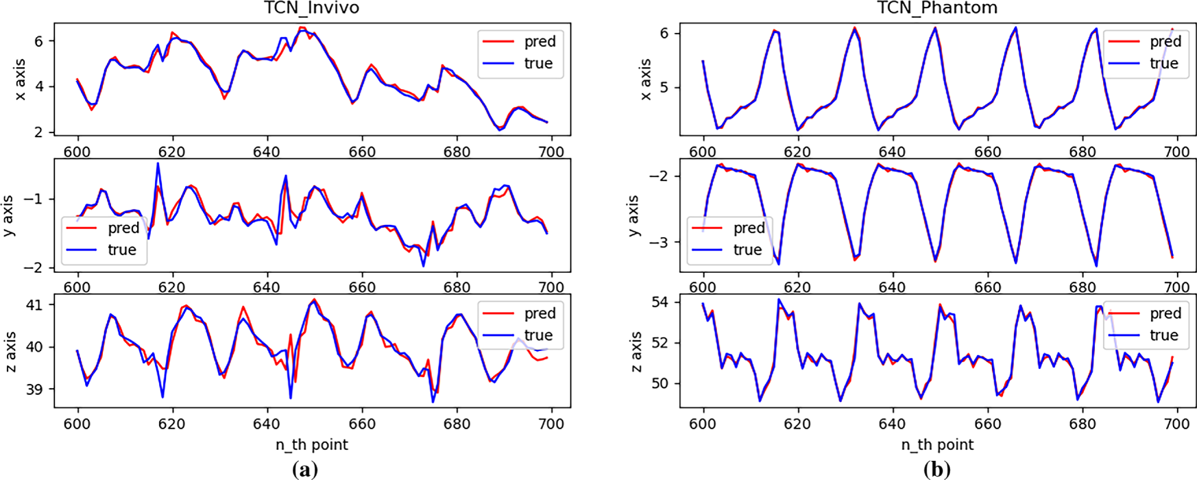
Figure 11: Single-step prediction effect with TCN: (a) In vivo; (b) Phantom datasets

Fig. 11 shows that, across different datasets, the TCN performs well in single-step predictions, effectively learning the magnitude and patterns of motion in all directions. However, at some inflection points in the trajectory, the prediction performance is relatively poor, with errors greater than those observed for smooth motion.

As shown in Fig. 12, the MSE range for the Phantom dataset is 0 to 0.068 mm2, while the MSE range for the in vivo dataset is 0 to 0.77 mm2. The prediction error peak for the Phantom dataset is smaller, indicating that the network’s prediction accuracy is higher on more regular motion trajectories. Furthermore, within the respective error ranges for different datasets, the points with larger prediction errors correspond to the trajectory inflection points shown in Fig. 11. The more dramatic the trajectory changes, the larger the model’s prediction error. At other points where the trajectory changes more smoothly, the model’s prediction error is relatively stable and approaches 0.

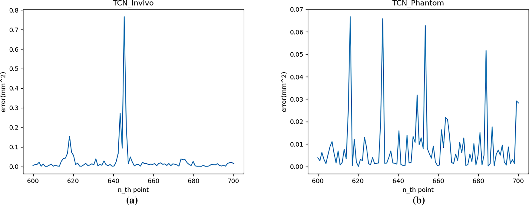
Figure 12: Single-step prediction error (MSE) with TCN: (a) In vivo; (b) Phantom datasets

Furthermore, statistical calculations show that the average single-step RMSE of the TCN model over a 100-step prediction range is 0.343 and 0.239 mm for the in vivo and Phantom datasets, respectively. This value is significantly lower than the statistical data for the autoregressive model, but higher than that of the LSTM network.

Fig. 13 shows the multi-step prediction errors of the TCN network for different step sizes on two datasets. This figure shows that for both the in vivo and Phantom datasets, the prediction error of the TCN network’s multi-step cyclic prediction is significantly greater than that of single-step prediction, and the RMSE increases significantly with increasing prediction steps (number of cycles). This is particularly evident in the in vivo dataset. In the more regular Phantom dataset, this change is less pronounced when the number of cycles increases from 5 to 20.

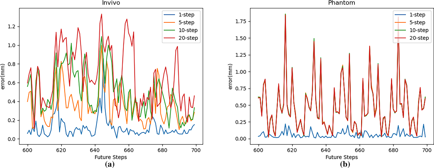
Figure 13: Multi-step prediction error (RMSE) with TCN: (a) In vivo; (b) Phantom datasets

Combined with the model’s single-step prediction results, because cyclic prediction uses predicted values rather than true values as model input, the prediction results obtained after each cycle will have cumulative error. On datasets with more regularity, the model’s single-step prediction error is smaller, and error accumulation is slower.

4.4 Prediction Phase Prediction Time Measurement

4.4.1 Prediction Time Statistics

The statistical process is consistent with the method used to inversely solve the kinematics of target points during tracking. By increasing the number of samples, the total time required to input all samples into each model and obtain a prediction result is calculated. The average value is used as the time required for the model’s single-step prediction to increase the reliability of the results.

The prediction time of each model is shown in Table 3. The data are all measured under the data scale of 650 ∗ 4, which means 650 4-step predictions are performed.

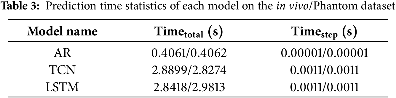
As shown in Table 3, the single-step inference time of the TCN and LSTM models was approximately 1.1 ± 0.1 ms, indicating negligible computational overhead relative to the system’s 25 Hz sampling period (40 ms).

To construct a complete latency profile of the teleoperation system, additional timing measurements were performed for the inverse-kinematics (IK) computation and mechanical actuation response stages. Table 4 shows the IK solving time represents the average computation required for forward and inverse joint transformations of the robot manipulator during each control cycle, whereas the response time (Table 5) quantifies the delay between command issuance and end-effector motion tracking.

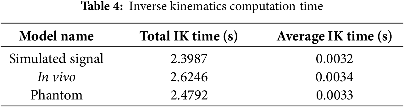
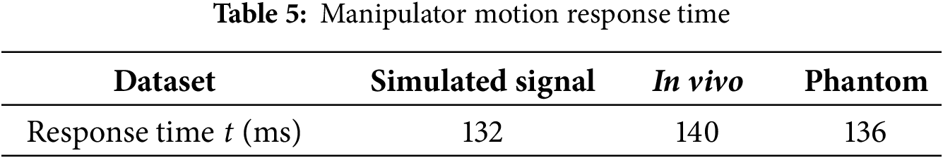
The results show that the average IK computation time was approximately 3.3 ms, while the mechanical actuation response ranged between 132–140 ms depending on the dataset. Together with the vision-based sensing delay (~18–20 ms) and model inference time (~1.1 ms), these measurements yield a total end-to-end latency of roughly 160 ± 5 ms, corresponding to about four sampling intervals at 25 Hz. Accordingly, the prediction horizon for all experiments was set to four discrete steps, ensuring complete compensation for the sensing-to-actuation delay of the teleoperation loop.

4.4.2 Compensation Time Calculation

After modeling the dynamic soft environment, the learned model can be used to predict the future target position during the robotic arm tracking process to compensate for tracking errors caused by time delays introduced by various links in the system. A schematic diagram of trajectory tracking is shown in Fig. 14, where the dotted line I represents the displacement after simulated camera positioning, the dashed line II represents the actual displacement of the point of interest, and the solid line III represents the displacement of the robotic arm end tracking the point of interest.

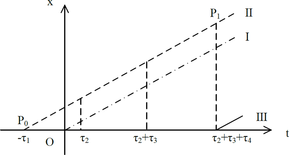
Figure 14: Schematic diagram of motion compensation teleoperation system delay

Using sensors to locate a point of interest (POI) takes a certain amount of time, τ1. The target pose is obtained by inverse kinematics to determine the joint target state, and motion commands are issued to move the robotic arm to the target point. These two processes take time τ3 and τ4, respectively. Therefore, as the robotic arm follows the POI, the position signal transmitted directly by the camera is actually the historical position of the POI. To achieve good tracking results, it is necessary to compensate for the system’s latency, which requires predicting the received signal. Assume that the network model takes time τ2 to predict the target point’s position.

When compensating for the lag in the movement of the robotic arm through model prediction, the calculation can be performed based on the single prediction time of the model. The calculation process is shown in Eq. (7).

{τall=τ1+τ2+τ3+τ4=τcycle⋅τstepτ2=step ⋅τcycle(7)

where τall is the sum of the lags introduced by each step in the control process. τstep is the time advance corresponding to the position predicted at each step in the prediction phase. τcycle is the time it takes the model to make one prediction. step is the number of prediction steps required in the prediction phase.

According to the above formula, the number of prediction steps for the in vivo and Phantom datasets is 4.71 and 4.61, respectively. If the required prediction step size is not an integer, you can use loop prediction to obtain integer-step prediction results (steps 4 and 5) around the ideal prediction step size. Then, interpolation processing is performed based on the actual situation to obtain prediction results for non-integer steps.

4.5 Model Motion Compensation Simulation Experiment

4.5.1 Experimental Procedure

Because the delays introduced by data processing/transmission, the robot’s motion to the target pose, and other stages vary with the specific setup, we adopt an online workflow that alternates data acquisition, model training, and model-based predictive control. The procedure is as follows:

Step 1: Read the ROI/target position data x0 at the dataset’s sampling frequency f=25 Hz to reproduce the original trajectory sampling rate.

Step 2: Add a reasonable artificial delay τc to emulate the time cost of binocular-camera observation and image processing of the ROI motion in the workspace; in our experiments, τc=40 ms.

Step 3: On the manipulator side, while receiving the ROI motion information, record the current end-effector position xe.

Step 4: Branching: if the collected data are fewer than N=600 samples, skip to Step (7). If enough data have been collected, execute Step (5). If the model has already been trained, execute Step (6).

Step 5: Train the model; once training is completed, return to Step (1).

Step 6: With the trained model, feed the received motion data into the predictor to obtain the model output xe′.

Step 7: Perform data processing on the manipulator side; compute the inverse kinematics for the point position to obtain the joint rotation angles and send the motion command to the robot.

Step 8: If the experiment has not finished, return to Step (1).

The overall tracking accuracy was evaluated using the cumulative root-mean-square tracking error (RMSE), defined as the square root of the mean squared Euclidean distance between the predicted and actual positions of the point of interest over N sampling steps, as shown in Eq. (8):

error=1N∑i=1n(pointi,pre−pointi,act)2(8)

where pointi,pre represents the i-th target position of the end of the robot arm; pointi,act represents the i-th actual position of the end of the robot arm

4.5.2 Analysis of the Results of Motion Compensation Using LSTM Model

Fig. 15 shows the robotic arm tracking performance using an LSTM model for motion compensation prediction. The blue line in the figure represents the change of target displacement over time, and the red line represents the change of displacement of the robotic arm end effector after motion compensation. As can be seen from the figure, achieving better motion compensation results with the LSTM model relies more on the regularity of the dataset itself. While the prediction performance on the Phantom dataset is acceptable, it performs poorly on the in vivo dataset. While some trends can be learned, there are still significant prediction errors.

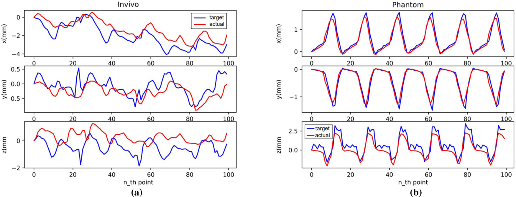
Figure 15: Motion compensation effect with LSTM: (a) In vivo; (b) Phantom datasets

Fig. 16 shows the cumulative average error curve for robotic arm tracking using the LSTM model for motion compensation prediction. As can be seen from the figure, during the motion compensation experiment, the error range for the in vivo dataset was 0 to 2.5 mm. The error range for the Phantom dataset was 0 to 1.9 mm, with the vast majority of data points falling between 0 and 1 mm. The motion compensation errors for most points were significant across different datasets.

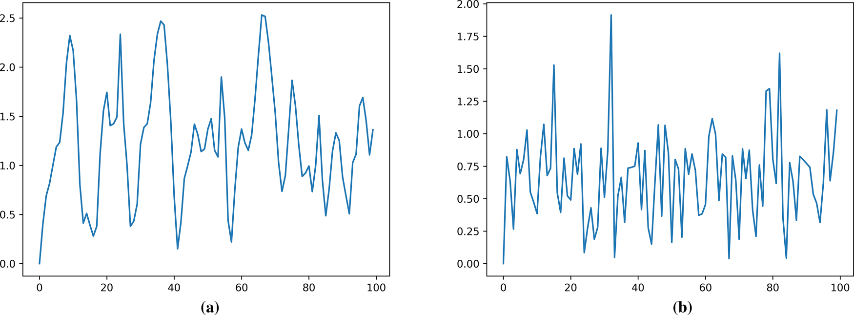
Figure 16: Motion compensation error (RMSE) with LSTM: (a) In vivo; (b) Phantom datasets

4.5.3 Analysis of the Results of Motion Compensation Using TCN Model

Fig. 17 shows the robotic arm tracking performance using the TCN model for motion-compensated prediction. The blue line in the figure represents the change of target displacement over time, and the red line represents the change of displacement of the robotic arm end effector after motion compensation. The figure shows that the TCN model has a strong learning ability for time series data with a certain regularity. It maintains relatively good prediction results in multi-step predictions with a short number of steps, with prediction performance far exceeding that of the autoregressive model.

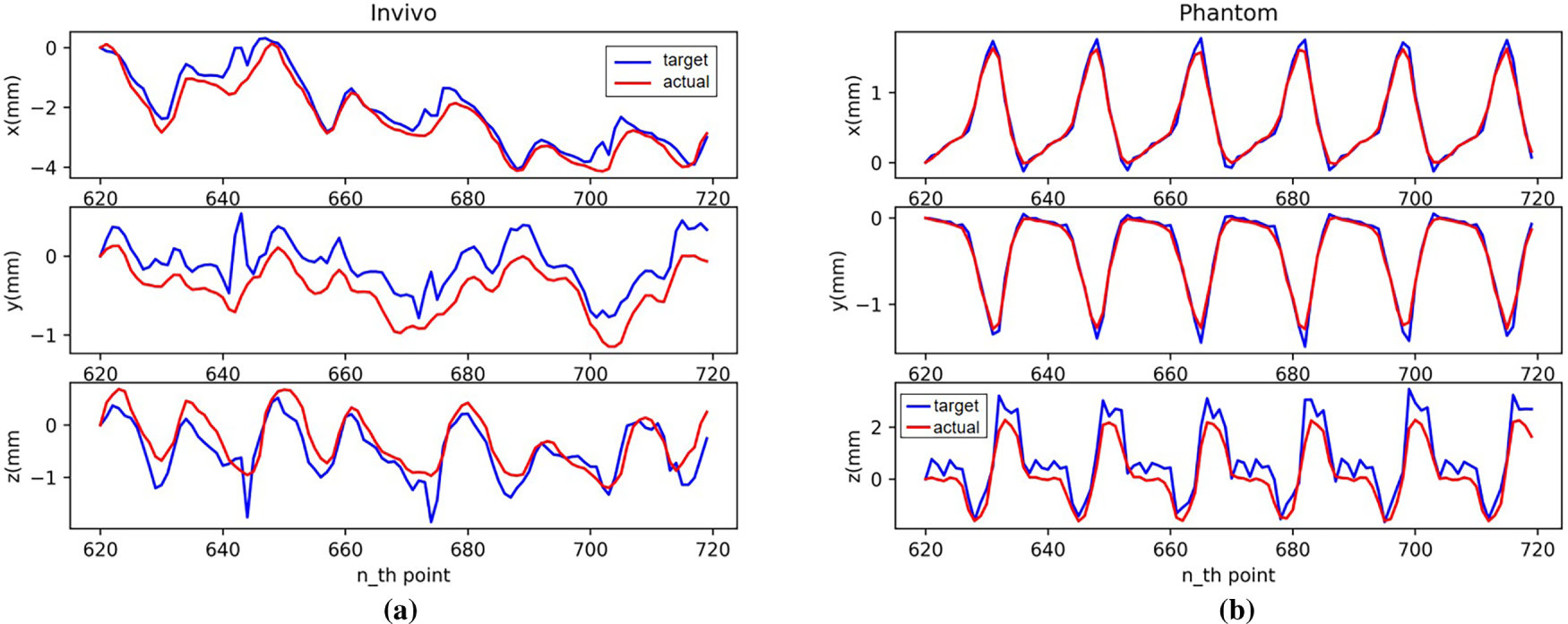
Figure 17: Motion compensation effect with TCN: (a) In vivo; (b) Phantom datasets

Fig. 18 shows the cumulative average error curve for robotic arm tracking using the TCN model for motion-compensated prediction. The figure shows that the prediction performance is good at most times across different data sets, as evidenced by low error values and when the error is decreasing. The curve indicates that the cumulative average error mostly falls within a small range of 0 to 1 mm.

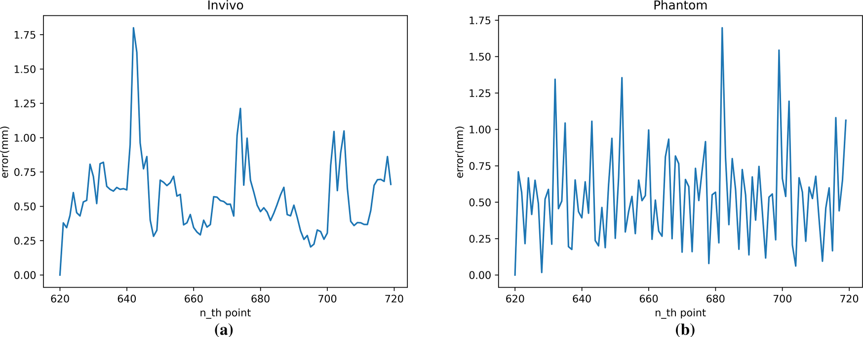
Figure 18: Motion compensation error (RMSE) with TCN: (a) In vivo; (b) Phantom datasets

Combining Figs. 17 and 18, we can see that the largest errors occur when the trajectory in the dataset changes dramatically, requiring the robotic arm to accelerate and decelerate at high speeds. After these moments, the robotic arm’s motion compensation performance recovers, and the prediction error returns to a lower level.

5  Discussion

Soft-tissue motion prediction plays a crucial role in robotic teleoperation, particularly in medical scenarios such as ultrasound-guided interventions and beating-heart surgeries. Latency induced by perception, inference, and actuation pipelines introduces phase delays and position errors that significantly affect the safety and accuracy of closed-loop control systems. To address this, learning-based motion prediction methods, particularly sequence models like LSTM networks and TCN, have been widely explored in recent literature. LSTM networks are capable of capturing long-term temporal dependencies and have demonstrated effectiveness in modeling quasi-periodic physiological motion such as heartbeat and respiration. However, their inherent sequential structure limits inference speed, posing challenges for real-time teleoperation systems where rapid response is required. In contrast, TCNs leverage dilated and causal convolutions to achieve large receptive fields with faster, parallelizable computation. This makes TCNs attractive candidates for motion compensation in systems that demand both low-latency and high-throughput performance.

Our experimental findings align with this trend. Among the three models tested the autoregressive baseline demonstrated limited applicability due to its linear assumptions and poor adaptability to nonlinear or high-frequency motion. LSTM performed significantly better than auto regressive model, particularly on the phantom dataset with its more regular and periodic trajectories. However, in the more complex in vivo dataset, where heartbeat and respiration overlapped and introduced abrupt motion changes, the LSTM exhibited error accumulation and reduced stability. TCN consistently achieved better performance in both single-step and short-horizon multi-step predictions, effectively capturing local trajectory patterns and delivering faster inference. These attributes are particularly beneficial when the prediction must compensate for a fixed system delay across sensing, inverse kinematics, and execution.

Despite its advantages, the proposed TCN-based approach presents several limitations. First, the model’s predictive performance depends heavily on the temporal regularity of the input data. While this is suitable for controlled phantom environments, it may not generalize well to scenarios involving arrhythmias, sudden occlusions, or irregular surgical manipulations, which frequently occur in real clinical practice. This was reflected in the increased prediction errors observed at trajectory inflection points in the in vivo dataset. Second, although TCNs are designed to capture local variations, they still struggle to maintain accuracy at kinks or high-acceleration segments, where motion dynamics change rapidly. These regions consistently showed higher error peaks across all models.

Another limitation lies in the exclusive use of positional trajectory data. The model does not use multimodal inputs such as visual textures, force feedback, or depth information, which are increasingly recognized as important cues in understanding soft-tissue deformation. Studies have shown that combining RGB imagery and depth data improves model robustness under complex lighting conditions, occlusions, and specular reflections. Additionally, the latency compensation mechanism in this study assumes a fixed prediction horizon, statically derived from offline measurements of system delay. In real deployments, however, delays can fluctuate due to varying computational loads or network latency. The absence of adaptive latency tracking may lead to horizon mismatch and degraded control performance in practice. Since multimodal data requires additional noise handling and synchronization, it would involve entirely different experiments and other research issues, causing this paper to deviate from its core focus. Therefore, the research on multimodal inputs will serve as a crucial direction for future work.

Finally, while the experiments employed real surgical datasets from the Da Vinci system, they were conducted entirely in an open-loop manner. The predictive models were evaluated offline, where recorded trajectories served as input and no real-time feedback from the robotic manipulator was involved. Consequently, the current validation primarily reflects the algorithm’s prediction accuracy rather than its dynamic control behavior. In contrast, a closed-loop or hardware-in-the-loop (HIL) framework would allow the predictive model to directly interact with the robotic system, enabling assessment of stability and robustness under real-time latency and jitter conditions. Although such validation has not yet been implemented, the present open-loop design reproduces the full sensing–inference–actuation delay chain (approximately 160 ms) and provides a functionally equivalent analysis of compensation accuracy.

Future work will extend this framework to real-time closed-loop testing with injected delay jitter to further evaluate the model’s robustness under dynamic teleoperation conditions. In addition, an adaptive delay monitoring module based on Kalman filtering, integration of multimodal sensory feedback, and evaluation under human-in-the-loop teleoperation will be pursued. Moreover, exploring hybrid architectures that combine TCNs with attention mechanisms or transformer-based encoders may enhance the capacity to handle temporal discontinuities and improve generalization across variable motion patterns.

6  Conclusions

In this work, we addressed the critical problem of latency-induced tracking errors in soft-tissue motion during robotic teleoperation by proposing a learning-based prediction framework. We decomposed the end-to-end system delay into distinct components—sensing, inference, inverse kinematics, and actuation—and derived an optimal prediction horizon to align the predicted target position with the actual control execution time. To achieve robust motion prediction, we evaluated three models on both synthetic and real-world datasets that capture heartbeat and respiratory dynamics.

Comprehensive experiments demonstrated that while the AR model is computationally efficient, it lacks the flexibility to model nonlinear or irregular motion. LSTM networks showed improved accuracy, particularly on regular trajectories, but suffered from error accumulation in multi-step forecasting. TCN models outperformed both baselines in terms of prediction accuracy, inference speed, and robustness to local trajectory changes, making them well-suited for real-time latency compensation in dynamic surgical environments.

Furthermore, we validated the proposed framework within a simulated teleoperation platform and demonstrated its capacity to reduce steady-state and peak tracking errors, especially in the presence of physiological motion. The integration of prediction and control under a latency-aware architecture offers a practical and effective solution for real-time soft-tissue tracking.

Acknowledgement: We would like to express our gratitude to Yakun Sun, Jiawei Tian for their support and assistance in aspects such as data organization, data preprocessing, experiments, and inspections.

Funding Statement: Support by Sichuan Science and Technology Program [2023YFSY0026, 2023YFH0004] and Guangzhou Huashang University [2024HSZD01, HS2023JYSZH01].

Author Contributions: Conceptualization: Bo Yang and Wenfeng Zheng; methodology: Siyu Lu and Guangyu Xu; software: Bo Yang and Siyu Lu; validation: Guangyu Xu and Yuxin Liu; formal analysis: Siyu Lu and Junmin Lyu; investigation: Guangyu Xu and Junmin Lyu; resources: Wenfeng Zheng and Bo Yang; data curation: Chao Liu and Yuxin Liu; writing—original draft preparation: Guangyu Xu, Wenfeng Zheng and Siyu Lu; writing—review and editing: Guangyu Xu, Wenfeng Zheng and Siyu Lu; visualization: Chao Liu, Guangyu Xu and Junmin Lyu; supervision: Bo Yang; project administration: Wenfeng Zheng; funding acquisition: Wenfeng Zheng. All authors reviewed the results and approved the final version of themanuscript.

Availability of Data and Materials: The datasetsare explained and referenced in Sections 3.1.1 and 3.1.2.

Ethics Approval: Not applicable.

Conflicts of Interest: The authors declare no conflicts of interest to report regarding the present study.

References

1. Mehrdad S, Liu F, Pham MT, Lelevé A, Atashzar SF. Review of advanced medical telerobots. Appl Sci. 2021;11(1):209. doi:10.3390/app11010209. [Google Scholar] [CrossRef]

2. Patel RV, Atashzar SF, Tavakoli M. Haptic feedback and force-based teleoperation in surgical robotics. Proc IEEE. 2022;110(7):1012–27. doi:10.1109/jproc.2022.3180052. [Google Scholar] [CrossRef]

3. Rahman MM, Balakuntala MV, Gonzalez G, Agarwal M, Kaur U, Venkatesh VLN, et al. SARTRES: a semi-autonomous robot teleoperation environment for surgery. Comput Meth Biomech Biomed Eng Imag Vis. 2021;9(4):376–83. doi:10.1080/21681163.2020.1834878. [Google Scholar] [CrossRef]

4. Dupont PE, Degirmenci A. The grand challenges of learning medical robot autonomy. Sci Robot. 2025;10(104):eadz8279. doi:10.1126/scirobotics.adz8279. [Google Scholar] [PubMed] [CrossRef]

5. Fu J, Maimone G, Iovene E, Zhao J, Redaelli A, Ferrigno G, et al. Human-inspired active compliant and passive shared control framework for robotic contact-rich tasks in medical applications. IEEE Trans Robot. 2025;41:2549–68. doi:10.1109/tro.2025.3548493. [Google Scholar] [CrossRef]

6. Noguera Cundar A, Fotouhi R, Ochitwa Z, Obaid H. Quantifying the effects of network latency for a teleoperated robot. Sensors. 2023;23(20):8438. doi:10.3390/s23208438. [Google Scholar] [PubMed] [CrossRef]

7. Farajiparvar P, Ying H, Pandya A. A brief survey of telerobotic time delay mitigation. Front Robot AI. 2020;7:578805. doi:10.3389/frobt.2020.578805. [Google Scholar] [PubMed] [CrossRef]

8. Yang B, Zhou Y, Tian J, Zhang X, Guo F, Liu S. A computational modeling approach for joint calibration of low-deviation surgical instruments. Comput Model Eng Sci. 2025;145(2):2253–76. doi:10.32604/cmes.2025.072031. [Google Scholar] [CrossRef]

9. Luo J, Huang D, Li Y, Yang C. Trajectory online adaption based on human motion prediction for teleoperation. IEEE Trans Autom Sci Eng. 2022;19(4):3184–91. doi:10.1109/TASE.2021.3111678. [Google Scholar] [CrossRef]

10. Cheng L, Tavakoli M. Neural network-based physiological organ motion prediction and robot impedance control for teleoperated beating-heart surgery. Biomed Signal Process Control. 2021;66(2):102423. doi:10.1016/j.bspc.2021.102423. [Google Scholar] [CrossRef]

11. Moniruzzaman MD, Rassau A, Chai D, Islam SMS. Long future frame prediction using optical flow-informed deep neural networks for enhancement of robotic teleoperation in high latency environments. J Field Robot. 2023;40(2):393–425. doi:10.1002/rob.22135. [Google Scholar] [CrossRef]

12. Tuna EE, Franke TJ, Bebek O, Shiose A, Fukamachi K, Cavuşoğlu MC. Heart motion prediction based on adaptive estimation algorithms for robotic assisted beating heart surgery. IEEE Trans Robot. 2013;29(1):261–76. doi:10.1109/TRO.2012.2217676. [Google Scholar] [PubMed] [CrossRef]

13. Yang B, Wong WK, Liu C, Poignet P. 3D soft-tissue tracking using spatial-color joint probability distribution and thin-plate spline model. Pattern Recognit. 2014;47(9):2962–73. doi:10.1016/j.patcog.2014.03.020. [Google Scholar] [CrossRef]

14. Yang B, Liu C, Poignet P, Zheng W, Liu S. Motion prediction using dual Kalman filter for robust beating heart tracking. In: Proceedings of the 2015 37th Annual International Conference of the IEEE Engineering in Medicine and Biology Society (EMBC); 2015 Aug 25–29; Milan, Italy. p. 4875–8. doi:10.1109/embc.2015.7319485. [Google Scholar] [PubMed] [CrossRef]

15. Yang B, Liu C, Zheng W, Liu S. Motion prediction via online instantaneous frequency estimation for vision-based beating heart tracking. Inf Fusion. 2017;35(10):58–67. doi:10.1016/j.inffus.2016.09.004. [Google Scholar] [CrossRef]

16. Zhang W, Yao G, Yang B, Zheng W, Liu C. Motion prediction of beating heart using spatio-temporal LSTM. IEEE Signal Process Lett. 2022;29:787–91. doi:10.1109/lsp.2022.3154317. [Google Scholar] [CrossRef]

17. Noroozi F, Daneshmand M, Fiorini P. Conventional, heuristic and learning-based robot motion planning: reviewing frameworks of current practical significance. Machines. 2023;11(7):722. doi:10.3390/machines11070722. [Google Scholar] [CrossRef]

18. Han L, Cheng L, Li H, Zou Y, Qin S, Zhou M. Hierarchical optimization for personalized hand and wrist musculoskeletal modeling and motion estimation. IEEE Trans Biomed Eng. 2025;72(1):454–65. doi:10.1109/TBME.2024.3456235. [Google Scholar] [PubMed] [CrossRef]

19. Liu Z, Wu S, Jin S, Ji S, Liu Q, Lu S, et al. Investigating pose representations and motion contexts modeling for 3D motion prediction. IEEE Trans Pattern Anal Mach Intell. 2023;45(1):681–97. doi:10.1109/TPAMI.2021.3139918. [Google Scholar] [PubMed] [CrossRef]

20. Hutchinson K, Reyes I, Li Z, Alemzadeh H. Evaluating the task generalization of temporal convolutional networks for surgical gesture and motion recognition using kinematic data. IEEE Robot Autom Lett. 2023;8(8):5132–9. doi:10.1109/lra.2023.3292581. [Google Scholar] [CrossRef]

21. Andrade-Ambriz YA, Ledesma S, Ibarra-Manzano MA, Oros-Flores MI, Almanza-Ojeda DL. Human activity recognition using temporal convolutional neural network architecture. Expert Syst Appl. 2022;191(6):116287. doi:10.1016/j.eswa.2021.116287. [Google Scholar] [CrossRef]

22. Lin CL, Lin FY, Huang CY, Ho YH, Chiu WC, Sung PS. Classification of gaits with a high risk of falling using a head-mounted device with a temporal convolutional network. IEEE Sens Lett. 2024;8(5):1–4. doi:10.1109/lsens.2024.3389675. [Google Scholar] [CrossRef]

23. Jiang Y, Peng B, Tian K, Wang L, Yuan Z. Visual autoregressive modeling: scalable image generation via next-scale prediction. In: Proceedings of the Advances in Neural Information Processing Systems 37; 2024 Dec 10–15; Vancouver, BC, Canada. San Diego, CA, USA: Inc. (NeurIPS); 2024. p. 84839–65. doi:10.52202/079017-2694. [Google Scholar] [CrossRef]

24. Staffini A, Svensson T, Chung UI, Svensson AK. Heart rate modeling and prediction using autoregressive models and deep learning. Sensors. 2021;22(1):34. doi:10.3390/s22010034. [Google Scholar] [PubMed] [CrossRef]

25. Al-Selwi SM, Hassan MF, Abdulkadir SJ, Muneer A, Sumiea EH, Alqushaibi A, et al. RNN-LSTM: from applications to modeling techniques and beyond—systematic review. J King Saud Univ Comput Inf Sci. 2024;36(5):102068. doi:10.1016/j.jksuci.2024.102068. [Google Scholar] [CrossRef]

26. Zhao Y, Ren J, Zhang B, Wu J, Lyu Y. An explainable attention-based TCN heartbeats classification model for arrhythmia detection. Biomed Signal Process Control. 2023;80(7):104337. doi:10.1016/j.bspc.2022.104337. [Google Scholar] [CrossRef]

27. Ginhoux R, Gangloff J, De Mathelin M, Soler L, Sanchez MMA, Marescaux J. Active filtering of physiological motion in robotized surgery using predictive control. IEEE Trans Robot. 2005;21(1):67–79. doi:10.1109/tro.2004.833812. [Google Scholar] [CrossRef]

28. Liang B, Gong G, Tong Y, Wang L, Su Y, Wang H, et al. Quantitative analysis of the impact of respiratory state on the heartbeat-induced movements of the heart and its substructures. Radiat Oncol. 2024;19(1):18. doi:10.1186/s13014-023-02396-0. [Google Scholar] [PubMed] [CrossRef]

29. Stoyanov D, Scarzanella MV, Pratt P, Yang GZ. Real-time stereo reconstruction in robotically assisted minimally invasive surgery. In: Medical Image Computing and Computer-Assisted Intervention—MICCAI 2010. Berlin/Heidelberg, Germany: Springer; 2010. p. 275–82. doi:10.1007/978-3-642-15705-9_34. [Google Scholar] [PubMed] [CrossRef]

30. Stoyanov D, Mylonas GP, Deligianni F, Darzi A, Yang GZ. Soft-tissue motion tracking and structure estimation for robotic assisted MIS procedures. In: Medical Image Computing and Computer-Assisted Intervention—MICCAI 2005. Berlin/Heidelberg, Germany: Springer; 2005. p. 139–46. doi:10.1007/11566489_18. [Google Scholar] [PubMed] [CrossRef]