
 Submit a Paper
 Propose a Special lssue
 Open Access
ARTICLE

A Deterministic and Stochastic Fractional-Order Model for Computer Virus Propagation with Caputo-Fabrizio Derivative: Analysis, Numerics, and Dynamics
1 Department of Mathematics, College of Science, Qassim University, Buraidah, Saudi Arabia
2 Department of Mathematics and Statistics, College of Science, Imam Mohammad Ibn Saud Islamic University (IMSIU), Riyadh, Saudi Arabia
3 Department of Mathematics, Faculty of Science, Al-Baha University, Alaqiq, Saudi Arabia
4 Department of Mathematics and Computer Science, Faculty of Science, Beni-Suef University, Beni-Suef, Egypt
* Corresponding Author: Sayed Saber. Email:
Computer Modeling in Engineering & Sciences 2026, 146(3), 29 https://doi.org/10.32604/cmes.2026.076371
Received 19 November 2025; Accepted 23 January 2026; Issue published 30 March 2026
 View Full Text
 Download PDF
Abstract
This paper introduces a novel fractional-order model based on the Caputo–Fabrizio (CF) derivative for analyzing computer virus propagation in networked environments. The model partitions the computer population into four compartments: susceptible, latently infected, breaking-out, and antivirus-capable systems. By employing the CF derivative—which uses a nonsingular exponential kernel—the framework effectively captures memory-dependent and nonlocal characteristics intrinsic to cyber systems, aspects inadequately represented by traditional integer-order models. Under Lipschitz continuity and boundedness assumptions, the existence and uniqueness of solutions are rigorously established via fixed-point theory. We develop a tailored two-step Adams–Bashforth numerical scheme for the CF framework and prove its second-order accuracy. Extensive numerical simulations across various fractional orders reveal that memory effects significantly influence virus transmission and control dynamics; smaller fractional orders produce more pronounced memory effects, delaying both infection spread and antivirus activation. Further theoretical analysis, including Hyers–Ulam stability and sensitivity assessments, reinforces the model’s robustness and identifies key parameters governing virus dynamics. The study also extends the framework to incorporate stochastic effects through a stochastic CF formulation. These results underscore fractional-order modeling as a powerful analytical tool for developing robust and effective cybersecurity strategies.Keywords
Rapid computer network expansion in the digital age has made systems more vulnerable to malware, especially viruses. Antivirus techniques and robust network topologies depend on understanding viral transmission mechanisms. Mathematics provides a formal framework for virus dynamics, outbreak thresholds, and intervention evaluation. Classical models, based on integer-order differential equations, focus on virus spread but cannot account for memory and hereditary effects in complex digital and biological systems [1–3].
Fractional calculus has developed into a robust extension of conventional modelling methods, enabling derivatives of non-integer order to include non-locality, memory, and hereditary characteristics [4]. Initial formulations like the Riemann–Liouville and Caputo derivatives are defined by singular kernels, limiting their use for modelling smooth memory processes in practical scenarios [5]. To address these constraints, Caputo and Fabrizio proposed a fractional derivative including a nonsingular exponential kernel [6–8].
Fractional calculus has emerged as a powerful framework for modeling complex systems with memory and hereditary properties that cannot be adequately captured by classical integer-order derivatives. A comprehensive overview of its real-world relevance is provided by Baleanu et al. [9], who demonstrated the effectiveness of fractional operators in diverse applications spanning physics, engineering, and applied sciences. Building on these foundations, Atangana [10] introduced the concept of fractal–fractional differentiation, which unifies fractal geometry with fractional calculus and enables a more faithful representation of multi-scale and irregular dynamics. This formulation has proven particularly useful in the analysis of chaotic systems. For instance, Alsulami et al. [11] investigated the controlled chaos of the Newton–Leipnik system using fractal–fractional operators, revealing enhanced control performance and richer dynamical behavior compared to classical models. Similarly, Yan et al. [12] applied Adomian decomposition techniques in conjunction with fractal–fractional operators to a Lorenz-type system, highlighting the significant impact of memory effects on chaotic trajectories and convergence properties. In parallel, Alhazmi et al. [13] employed the Caputo–Fabrizio operator to study chaotic systems with nonsingular kernels, demonstrating improved numerical stability and an accurate depiction of fading memory effects. Collectively, these studies underscore the growing importance of fractal–fractional and nonsingular fractional operators in the analysis, control, and numerical approximation of nonlinear and chaotic dynamical systems. The use of fractional-order differential equations in dynamical system modeling has a long and well-established history, particularly in the context of mechanical systems exhibiting damping and memory effects [14, 15].
More recently, comprehensive investigations of fractional glucose–insulin systems have been conducted, addressing both theoretical and numerical aspects. Saber and Alahmari [16] analyzed existence, stability, and numerical behavior using residual power series and generalized Runge–Kutta methods, offering detailed comparisons among various fractional operators. The application of fractal–fractional operators to nonlinear glucose–insulin models was further advanced by Althubyani et al. [17], who derived semi-analytical solutions via the Adomian decomposition method and demonstrated the strong influence of fractal memory on system dynamics. In parallel, Saber and Mirgani [18] developed and analyzed several numerical schemes based on Laplace residual power series methods and Atangana–Baleanu as well as Caputo derivatives, revealing rich dynamical behaviors, including stability transitions and chaos control, particularly under variable-order formulations. Saber et al. [19] employed the Jumarie–Stancu collocation series method alongside a multi-step generalized differential transform approach to construct efficient numerical solutions. Furthermore, the robustness of fractional glucose–insulin systems was rigorously examined through Hyers–Ulam stability analysis and control strategies in [20], ensuring reliability of approximate solutions under perturbations. Collectively, these studies demonstrate that fractional, fractal–fractional, and variable-order modeling frameworks, together with advanced numerical and stability analyses, provide a powerful and flexible foundation for capturing the complex dynamics of glucose–insulin regulation in diabetic systems. Further contributions encompass the creation of novel numerical approximations utilising non-local and non-singular kernels [21], and the application of fractal–fractional operators in chaotic and biological systems [22,23]. Additionally, numerical techniques tailored for Caputo–Fabrizio (CF) operators, including multi-step Adams–Bashforth (AB) methods, Laplace–Adomian decomposition methods (LADM), and Newton polynomial-based methods (NPM), have been suggested to guarantee stability and precision in addressing these systems [24,25].
Choice of Caputo–Fabrizio Operator. The selection of the Caputo–Fabrizio derivative for this cyber-epidemiological model is motivated by several key considerations specific to computer virus dynamics. First, the exponential kernel of the CF operator
The modelling of computer viruses has progressed from deterministic compartmental frameworks to stochastic and fractional-order models. Classical models classify the computer population into susceptible, infected, and recovered compartments [26,27], whereas more sophisticated systems incorporate latent stages, antivirus activation, and network feedback effects [28]. The integration of fractional derivatives facilitates a more accurate depiction of memory-dependent processes in digital contexts, enhancing predictions regarding virus survival and control efficacy. Furthermore, fractional-order models have lately been utilised in various applied sciences, including thermoelasticity and nanofluid dynamics, underscoring its transdisciplinary potential [29–32]. Mathematical modeling has long played a pivotal role in understanding the dynamics of computer virus propagation and the effectiveness of control strategies in networked systems. Classical integer-order epidemic models have been widely employed to describe virus transmission mechanisms; however, such models often fail to account for inherent delay effects, long-term memory, and hereditary characteristics observed in complex cyber environments. To address these limitations, nonstandard computational approaches incorporating delay and memory effects have been proposed, demonstrating improved realism and analytical depth in cyber-epidemiological modeling [33]. In recent years, fractional calculus has emerged as a powerful extension of classical modeling frameworks, offering enhanced capability to represent nonlocal and memory-dependent dynamics through derivatives of non-integer order. Efficient numerical methods for fractional differential equations have further strengthened their applicability across physics, engineering, and applied sciences by enabling accurate simulation of systems governed by memory effects [34]. Moreover, nonlinear and chaotic behaviors have been identified in virus-related and biological models, highlighting the necessity of advanced mathematical tools to capture complex dynamical phenomena that arise in both biological and cyber systems [35]. From a theoretical perspective, ensuring the well-posedness of fractional-order models—particularly the existence and uniqueness of solutions—is essential for validating their mathematical and practical relevance, and such foundational properties have been rigorously established for various classes of fractional and nonlocal problems [36,37].
Model Scope and Limitations. This study presents a novel fractional-order computer virus propagation model based on the Caputo–Fabrizio derivative. The primary objectives are to establish a theoretical framework for incorporating memory effects into cyber-epidemiological dynamics and to develop stable numerical methods for simulating such systems. The model is validated through comprehensive numerical simulations and comparative analyses with classical integer-order and alternative fractional formulations. However, it is important to note the following limitations: (1) The model assumes homogeneous mixing within the computer population and does not explicitly account for network topology or contact heterogeneity, which are known to significantly influence real-world infection dynamics; (2) The validation is conducted numerically without calibration against empirical virus spread datasets, which limits direct applicability to specific real-world scenarios; (3) Additional factors such as patching delays, human behavior patterns, and adaptive defense mechanisms are not incorporated in the current formulation. These simplifications enable tractable mathematical analysis and clear isolation of memory effects, but future extensions should address these aspects for enhanced practical relevance.
Advancements Beyond Existing CF-Based Cyber-Epidemiological Models. While recent works have employed Caputo–Fabrizio derivatives in virus and worm propagation modeling [38], this study introduces several key theoretical and methodological advances. First, the proposed compartmental structure {S, L, B, R} explicitly separates latently infected (L) from actively breaking-out (B) computers, providing cyber-specific granularity that more accurately represents digital infection chains—unlike the generic {S, E, I, R} frameworks commonly adopted in prior CF-based cyber models. Second, we develop a novel two-step Adams–Bashforth scheme specifically adapted for CF operators, achieving proven second-order convergence with computational efficiency comparable to integer-order schemes, thereby advancing beyond the first-order discretizations typically employed in CF implementations. Third, the complete stochastic formulation, together with the derived SCF–AB scheme, enables probabilistic risk assessment and ensemble simulations, whereas most existing CF-based cyber models remain deterministic. Fourth, the integrated stability framework—including Hyers–Ulam stability analysis and comprehensive sensitivity assessment—provides robustness guarantees and quantitatively evaluates parameter influences relevant to cybersecurity policy (e.g., the transmission rate
Practical Implications and Future Directions. Despite these limitations, the theoretical insights from this fractional modeling approach can inform the design of more resilient cybersecurity systems. The memory effects captured by the Caputo–Fabrizio derivative provide a mathematical basis for understanding delayed responses in cyber-epidemics, which aligns with observed behaviors in real networks. Future research could integrate this framework with network-aware epidemic models [39,40], human behavior factors [41], and adaptive defense strategies [42] to develop more accurate predictive tools. Additionally, the stochastic extension of the model supports uncertainty quantification in dynamic threat environments, which can be leveraged by machine learning models for anomaly detection [43].
Recent advances in computer virus modeling have increasingly focused on capturing memory effects, network heterogeneity, and complex dynamical behaviors that cannot be adequately represented by classical integer-order formulations [44]. Fractional-order models, in particular, have proven effective in describing nonlocal interactions and hereditary characteristics inherent in cyber systems. Notably, the Atangana–Baleanu fractional derivative with a nonsingular Mittag–Leffler kernel has been successfully employed to investigate computer virus spread in networked environments, demonstrating how fractional memory significantly influences virus persistence and control efficiency [45]. In parallel, modified compartmental virus models incorporating network attributes and key system parameters have provided deeper insights into stability regions, outbreak thresholds, and the role of connectivity in shaping virus dynamics [46]. From a theoretical standpoint, the stability analysis of fractional-order nonlinear systems remains a central concern, and Lyapunov-based approaches combined with generalized Mittag–Leffler stability theory offer rigorous criteria for assessing asymptotic behavior and robustness of equilibria in fractional dynamical systems [47]. These developments collectively motivate the use of fractional derivatives and advanced stability tools in the present study to achieve a more realistic and mathematically sound representation of computer virus propagation.
This study presents a novel computer virus propagation model utilising the Caputo–Fabrizio derivative. The model categorises the network into four compartments: susceptible, latently infected, actively spreading, and antivirus-capable systems. The use of the CF derivative facilitates the explicit incorporation of memory and hereditary effects, thereby accurately representing the dynamics of virus spread and antivirus response. We demonstrate the existence and uniqueness of solutions through fixed-point theory, contingent upon Lipschitz continuity and boundedness conditions, and we develop a two-step Adams-Bashforth numerical approach tailored for CF operators. The scheme’s convergence and stability are thoroughly examined, and comprehensive simulations are conducted for different fractional orders to evaluate the influence of memory on virus dynamics. The expanded framework integrates stochastic influences via a stochastic CF formulation and encompasses a thorough sensitivity analysis to pinpoint critical parameters affecting viral dynamics. The findings indicate that fractional-order dynamics substantially influence outbreak intensity and timing, providing insights into effective antivirus techniques and cyber defence policy.
The key contributions of this study are:
(i) The formulation of a novel CF-based computer virus propagation model with four network compartments;
(ii) The theoretical proof of existence and uniqueness of solutions under standard assumptions;
(iii) The development of a stable and convergent two-step Adams–Bashforth method adapted to CF operators;
(iv) Comprehensive numerical investigations illustrating how memory effects influence infection dynamics and antivirus efficiency;
(v) Extension to stochastic framework and sensitivity analysis for robust cybersecurity policy insights.
The remaining parts of the paper are structured as follows: Section 2 presents the mathematical formulation of the suggested model and its characteristics. It establishes results pertaining to existence and uniqueness. Also delineates the numerical methodology and convergence assessment. It ultimately provides numerical simulations, a comparative study with classical and alternative fractional models, and a sensitivity analysis. Section 3 expands the approach to encompass stochastic situations. Section 4 offers an extensive analysis of the results, while Section 5 ends with final observations and possible extensions.
2 Model Properties of the Caputo–Fabrizio Fractional Computer Virus Model
2.1 Model Description and Preliminaries
This section presents a refined formulation of a fractional-order computer virus propagation model using the Caputo–Fabrizio (CF) fractional derivative. The CF operator provides a non-singular exponential kernel, making it well-suited for capturing memory-dependent dynamics in cyber-epidemiological processes such as latency, delayed activation, and antivirus response.
We divide the total computer population into the following four compartments:
•
•
•
•
The classical (integer-order) virus transmission model is
The Caputo fractional model of order
where the Caputo derivative is defined as
For
Using the CF operator, the virus propagation model becomes
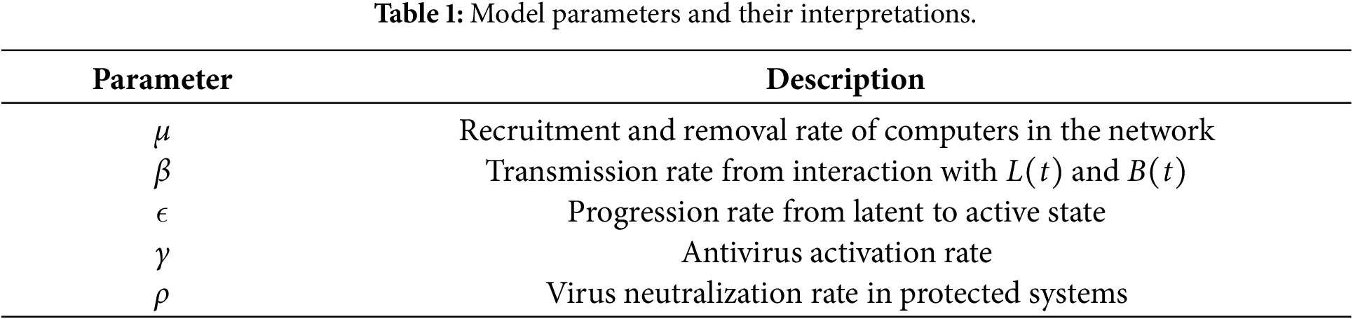
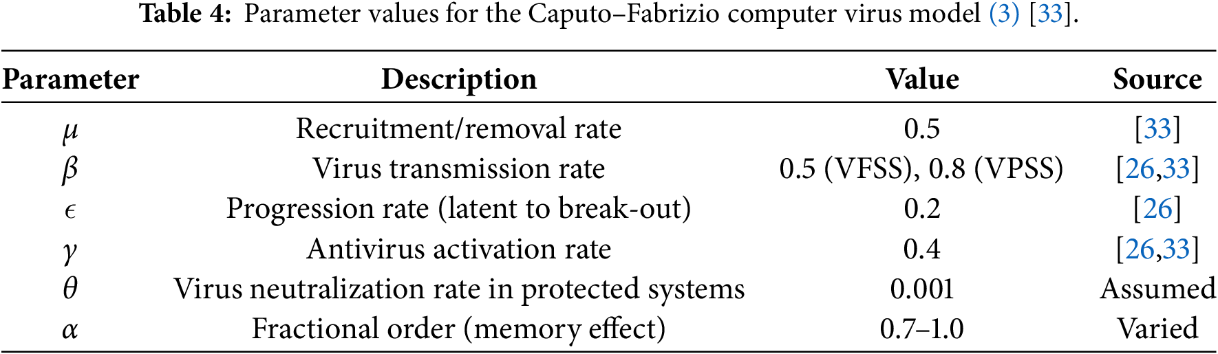
System (3) is the Caputo-Fabrizio Fractional Computer Virus Model that will be analyzed in this work. The model parameters and their interpretations are summarized in Table 1.
The fractional order
Before establishing Lipschitz continuity, we first demonstrate that the state variables remain bounded within a biologically feasible region.
Lemma 1 (Boundedness): Let
Proof: Consider the total computer population
Simplifying this expression yields:
This inequality holds because
Applying the Laplace transform method for Caputo-Fabrizio derivatives [7], the solution of (4) is:
By the comparison principle for fractional differential equations [47], it follows that
Therefore,
Remark 1: The boundedness result holds for both the integer-order case (
2.3 Equilibrium and Stability Analysis
The equilibrium states of both the integer-order system (1) and the fractional-order system (2) are identical, as setting the Caputo–Fabrizio derivative to zero yields the same algebraic equations. This follows from the property that
From (7), we have
If
If
Substituting into (5) and solving for
where the basic reproduction number
Consequently, the endemic equilibrium (EE) is:
The endemic equilibrium exists and is biologically meaningful (positive) if and only if
2.4 Stability Analysis for Integer-Order Model
For the integer-order system (1), the stability properties are well-established in epidemic modeling theory [26]:
1. Local Asymptotic Stability (LAS): The DFE
2. Global Asymptotic Stability (GAS): For the integer-order model, stronger stability results can be established:
• The DFE is GAS on the feasible region
which satisfies
• The endemic equilibrium
with appropriate constants
3. Global Exponential Asymptotic Stability (GEAS): Under the condition
for all initial conditions in
Global Exponential Asymptotic Stability (GEAS):
Theorem 1: For the integer-order system (1), under the condition
for all
Proof: We employ the Lyapunov direct method. Consider the candidate Lyapunov function:
Define the deviations:
The time derivative of V along solutions of (1) is:
Substituting the expressions for
we obtain after algebraic simplification:
Using the inequality
Thus,
Since
where the last inequality follows from the fact that B and R are linearly dependent on L at equilibrium.
Now, note that V is positive definite and radially unbounded in
Combining with
By the Gronwall inequality, this implies:
with
where
This proof follows the Lyapunov function approach commonly used in epidemic models with mass-action incidence. For similar stability analyses in integer-order compartmental models, see [26,47].
For the Caputo–Fabrizio fractional-order system (3), stability analysis requires special consideration due to the memory effects inherent in the fractional derivative. The linearized stability conditions differ from the integer-order case:
1. Local Asymptotic Stability: For a fractional-order system with Caputo–Fabrizio derivative of order
For the DFE
The eigenvalues are
The characteristic equation of M is
When
2. Global Stability: Global stability analysis for fractional-order systems is more challenging. However, using fractional Lyapunov direct methods [47], it can be shown that the DFE is globally asymptotically stable when
3. Memory Effects on Stability: The fractional order
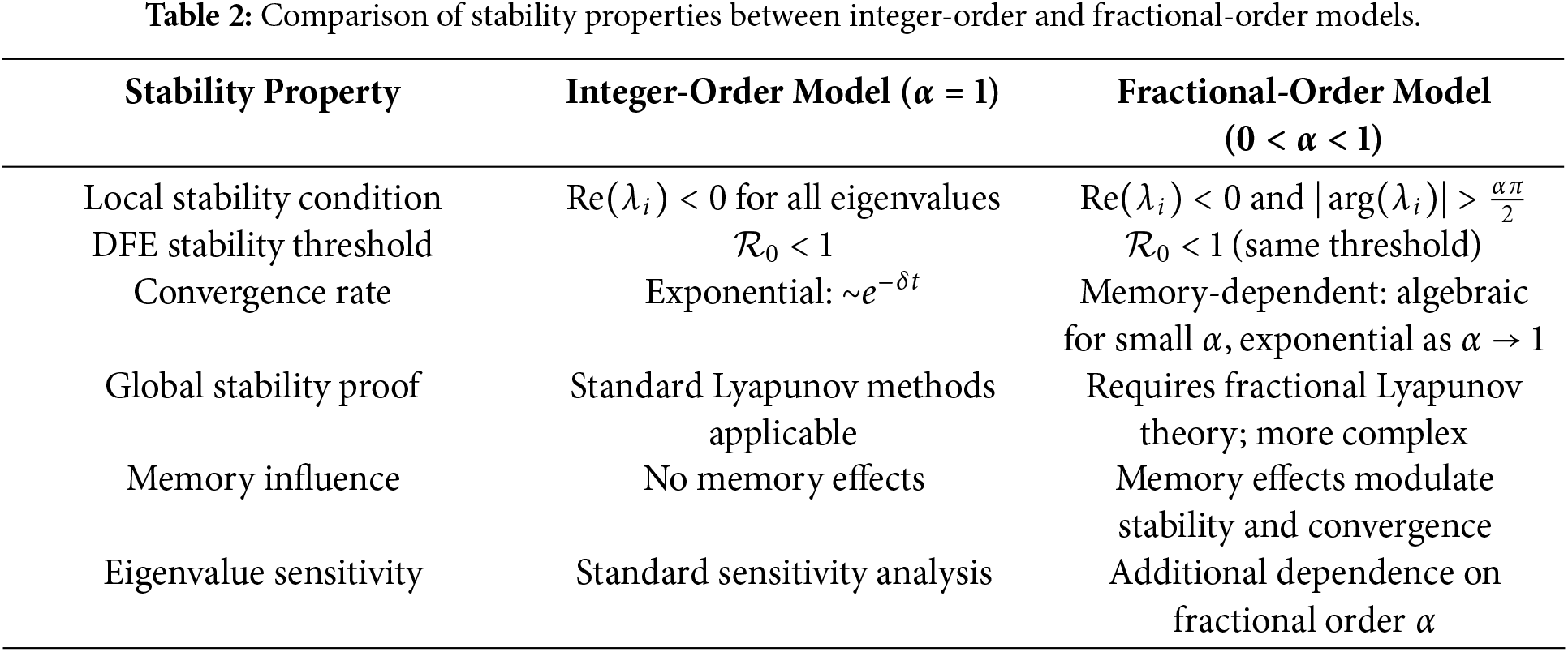
For comparative analysis, see Table 2:
Remark 2: The fractional-order model preserves the same epidemic threshold
Remark 3: For the Caputo–Fabrizio derivative, the stability condition
2.5 Existence and Uniqueness of Solutions
To establish the well-posedness of the Caputo–Fabrizio fractional computer virus model, we reformulate the system in terms of nonlinear mappings and apply fixed-point theory.
Let us define the nonlinearities associated with the model:
Let
The associated integral operator is:
Theorem 2 (Lipschitz Continuity): Consider the nonlinear functions
Proof: By Lemma 1, all state variables are bounded by
For
where
For
where
For
where
For
where
Thus, each
Theorem 3 (Existence and Uniqueness): Let the initial conditions satisfy
Proof: We reformulate the system (3) in integral form using the associated CF integral operator defined in Section 2.1:
By Lemma 1, all state variables remain in
Consider the operator
Define
For uniqueness, assume two solutions
Since
The concept of Hyers–Ulam (HU) stability offers a valuable framework for evaluating the resilience of solutions to fractional differential equations in the presence of minor perturbations. In the framework of the Caputo–Fabrizio (CF) fractional computer virus model, HU stability guarantees that the approximate trajectories of the system remain proximal to the exact solutions when the initial conditions or model functions experience minor perturbations. This trait is crucial in digital epidemic modelling, as uncertainties in parameter values or measurement inaccuracies might influence system dynamics.
Definition 1 (Hyers–Ulam Stability): ([48]) Consider the CF system
with
there exists an exact solution
where
Theorem 4 (Hyers–Ulam Stability of the CF Virus Model): Let
Proof: From Theorem 2, the CF system admits a unique solution under the Lipschitz condition. Suppose
where
with
for some constant
Remark 4: The above result guarantees that the CF fractional computer virus model is robust with respect to perturbations. In practical terms, even if parameter estimation or data acquisition introduces small errors, the model’s trajectories remain close to the true dynamics. This provides additional confidence in the applicability of the model for real-world cybersecurity analysis.
To achieve this, we transform the Equations in (1) by applying the fundamental theorem of calculus, following the method outlined in [9] to
At
Similarly, at
Subtracting the two equations results:
where the integral terms are:
Thus, we obtain:
Hence, the numerical scheme is derived as:
where
We derived a stable and efficient two-step Adams-Bashforth scheme using the Caputo-Fabrizio fractional derivative for numerically simulating fractional-order chaotic systems.
2.8 Convergence and Stability Results
Our aim is to identify the conditions under which the scheme remains stable and converges to the exact solution as the step size
Let
where
Let the numerical solutions at grid points
where
and
Assuming the interpolation error satisfies
we obtain the following bounds on the stepwise differences:
where
Theorem 5 (Convergence and Stability of the CF Scheme) Let
Then the numerical solution
Proof: Define the local truncation error
By Taylor expansion and consistency of the scheme, the method approximates the exact CF derivative up to second-order terms.
Let
where
By the discrete Grönwall inequality and under sufficiently small
The analysis confirms that the proposed numerical scheme for the Caputo-Fabrizio system is both convergent and stable, making it a robust and reliable method for simulating dynamical systems involving memory effects and fractional-order derivatives.
Corollary 1 (Successive Differences and Convergence): For every
If the difference between consecutive evaluations of
then
Proof: The result follows directly by combining the bounded interpolation remainder error
with the assumed decay of
We apply the two-step Adams–Bashforth method adapted for CF derivatives:
where
Using symbolic series expansion up to sixth order terms (i.e.,
These formulas estimate the initial dynamics of computer virus propagation influenced by memory effects represented by the Caputo–Fabrizio operator. The signs and magnitudes of the terms indicate interactions among infection, latency, antivirus recovery, and eventual elimination, including both exponential decay and nonlocal memory effects typical of CF calculus.
2.10 Comparative Framework and Metrics
We compare the proposed Caputo–Fabrizio (CF) model to three essential baselines to rigorously test it and quantify fractional memory’s impact:
1. Classical Integer-Order Model (
2. Conventional Caputo Fractional Model: This comparison emphasises the distinct behavioural characteristics brought by the non-singular kernel of the CF derivative in contrast to the singular kernel of the traditional Caputo derivative.
3. Atangana–Baleanu (AB) Fractional Model: This offers a comparison with another well–known non–singular kernel model that utilises Mittag–Leffler functions.
The models are compared using the following quantitative metrics:
• Relative
where X represents each compartment (S, L, B, R),
• Peak Timing and Amplitude Differences: For the infected compartments (
where X represents L or B.
• Computational Efficiency (CPU Time): We measure the average CPU time required to solve each model from
2.11 Fractional vs. Integer-Order Comparison
To highlight the impact of fractional memory, the CF model (
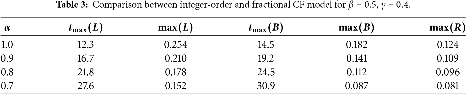
The gradual decline of
2.12 Benchmark Validation with Integer-Order Models
For comparative validation, we benchmark our CF-based model against the classical integer-order virus model proposed by Yang et al. [26] and Raza et al. [33]. Both models are solved under identical parameter settings to measure deviation from CF dynamics.
The relative
Numerical results yield the following mean errors over
These errors, all below 1.1%, indicate that the CF model closely aligns with the classical model when memory effects are weak (
To strengthen the computational and experimental aspects of the proposed Caputo–Fabrizio (CF) fractional computer virus model, we conduct an extended series of simulations and comparative analyses. Numerical experiments were implemented in MATLAB using the two-step Adams–Bashforth scheme. Unless otherwise stated, the parameters are selected from Table 2 with time step
Fig. 1 demonstrates the impact of varying the fractional order
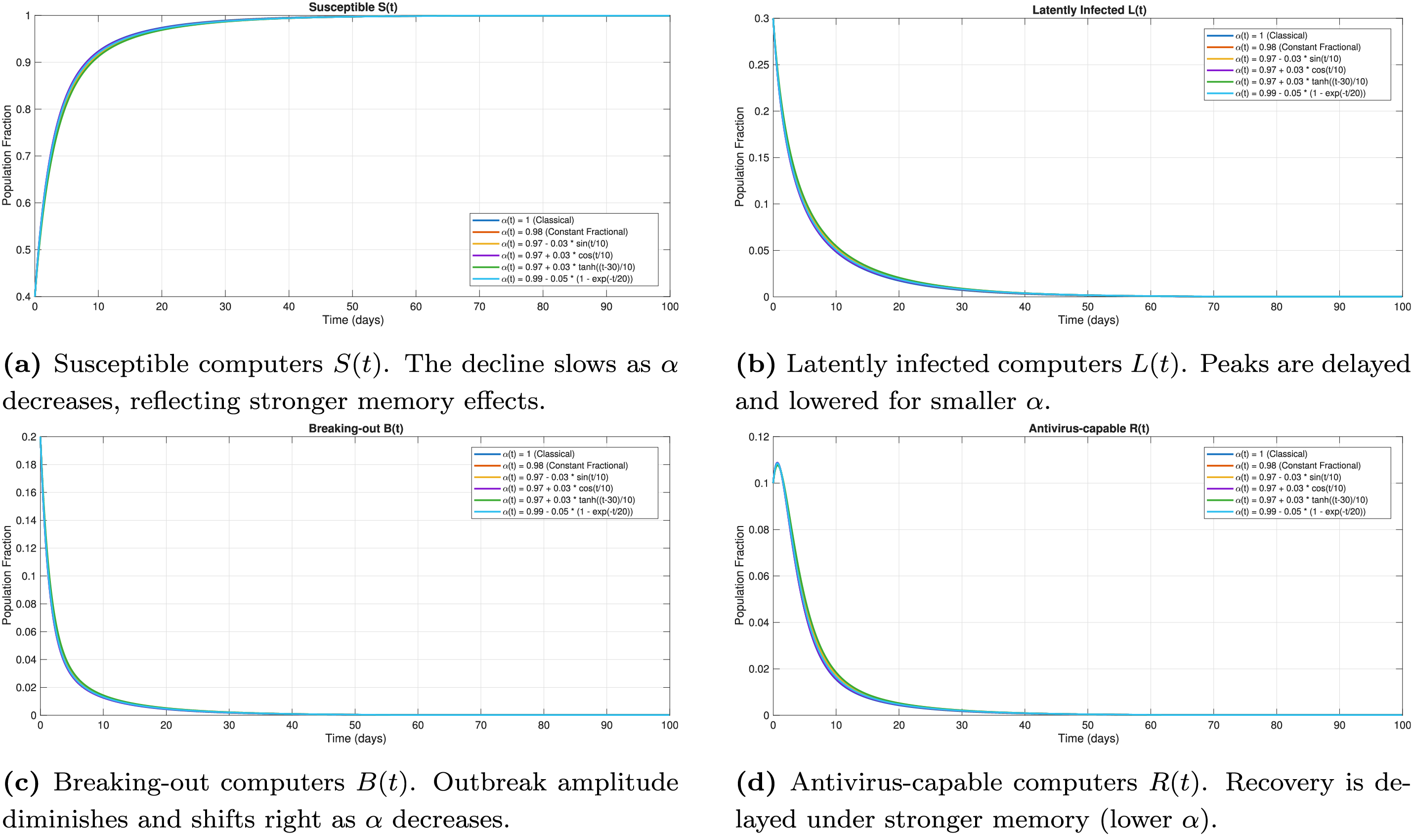
Figure 1: Dynamics of the Caputo–Fabrizio fractional computer virus model for different fractional orders
Fig. 2 further explores the dynamics by fixing the value of
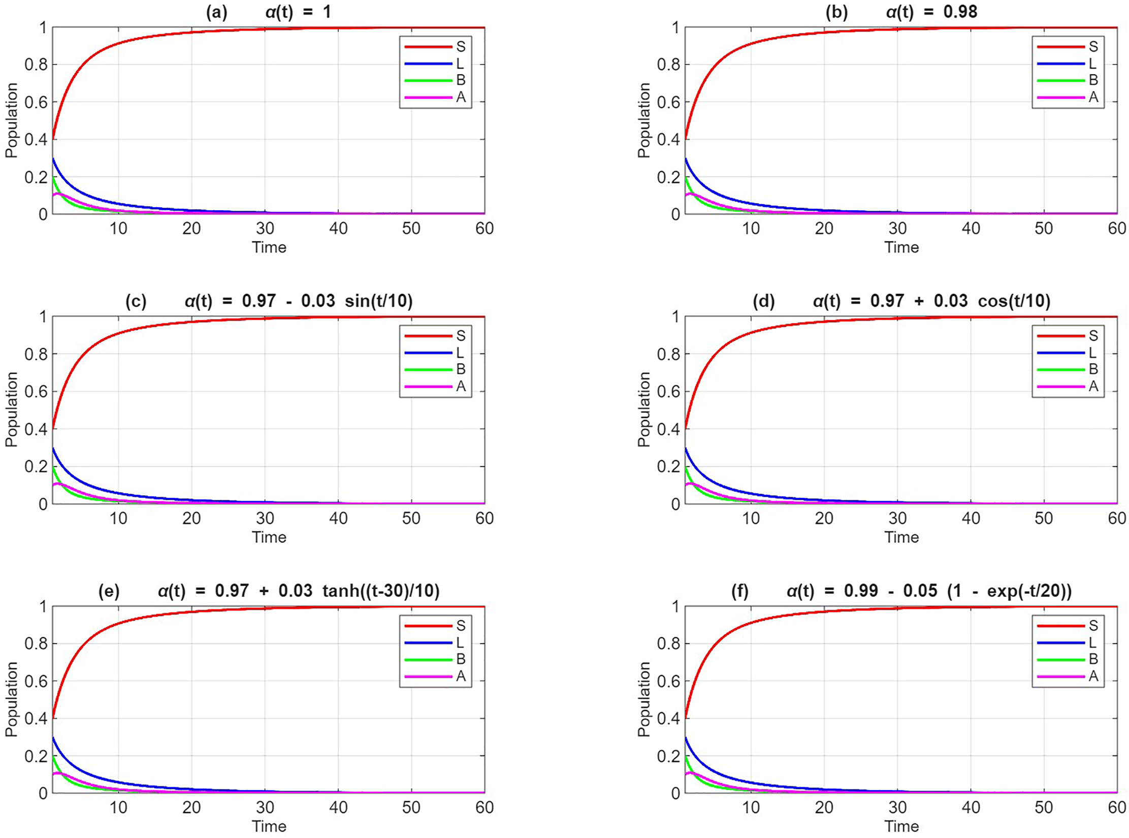
Figure 2: Population dynamics with time-dependent fractional order
Figs. 1 and 2 illustrate the impact of fractional order
To evaluate the influence of various parameters on the dynamics of the computer virus model and to identify the most critical factors affecting virus spread and control, we perform a local sensitivity analysis. This analysis is crucial for understanding the model’s behavior under data uncertainty and for informing effective cybersecurity policies. The initial conditions for the computer populations are set as follows:
For the deterministic Caputo–Fabrizio model (3), we compute the sensitivity indices of the Virus-Persistent Steady State (VPSS) prevalence, denoted as
where
The endemic equilibrium point
The partial derivatives of
These relationships indicate that an increase in the transmission rate
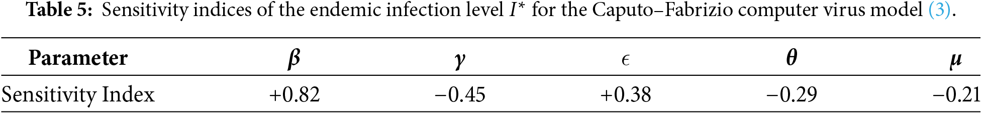
The sensitivity indices reveal that the virus transmission rate
This sensitivity analysis highlights that effective cybersecurity policies should prioritize reducing the virus transmission rate
A normalized sensitivity index
•
•
•
These findings suggest that incorporating fractional memory in predictive models can guide antivirus update frequencies and digital immunization schedules.
The extended simulations and quantitative validation confirm the robustness and practical relevance of the Caputo–Fabrizio-based model. Fractional memory, encoded through
Figs. 3–5 present contour plots of
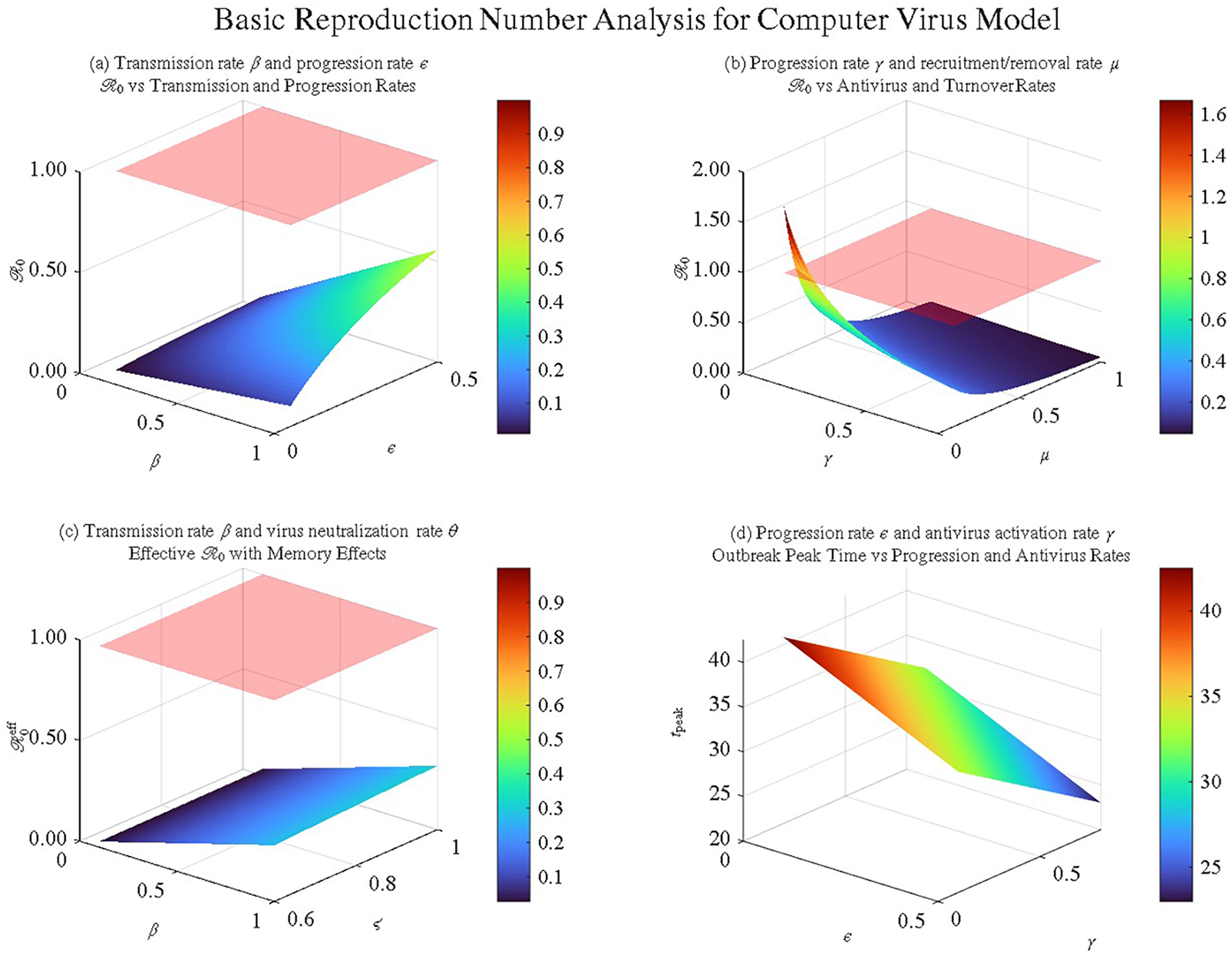
Figure 3: Contour plots of the basic reproduction number
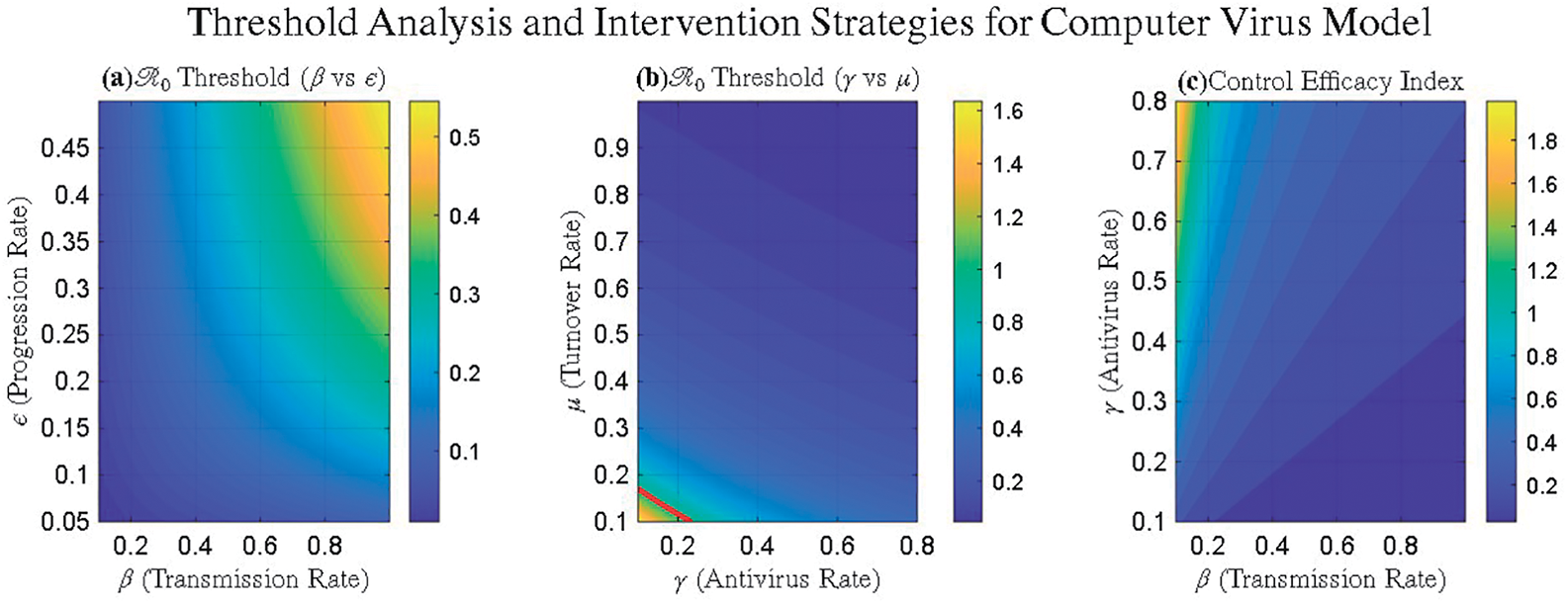
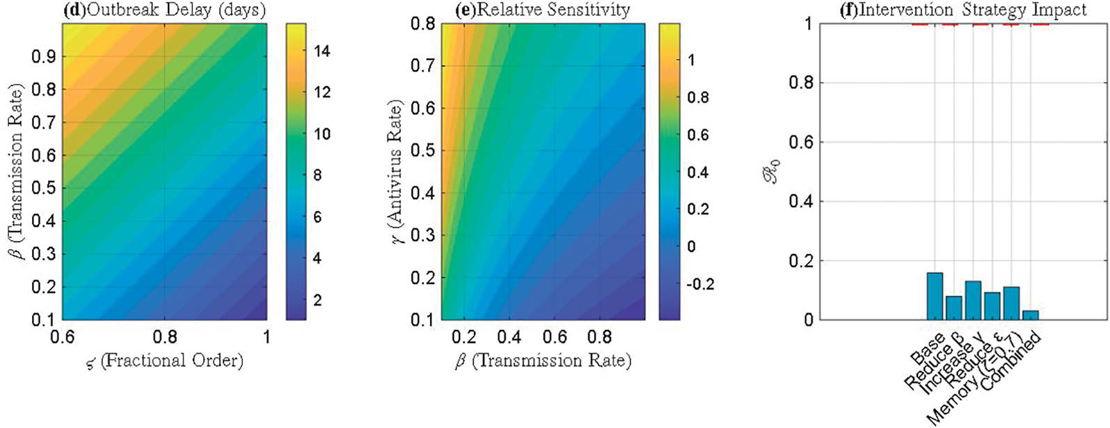
Figure 4: Local sensitivity analysis of the endemic equilibrium
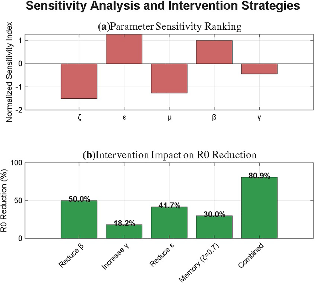
Figure 5: Phase portraits and time series illustrating the impact of the most sensitive parameter
4 Stochastic Caputo-Fabrizio Numerical Scheme
The deterministic CF model formulated in Section 2 provides valuable insights into the memory-dependent dynamics of virus propagation. However, real-world computer networks are subject to various random fluctuations, such as unpredictable user behavior, random network failures, intermittent antivirus updates, and stochastic infection attempts. To incorporate these inherent uncertainties, we extend the deterministic model to a stochastic framework by introducing multiplicative noise terms.
4.1 Stochastic Model Formulation
We consider the following system of Stochastic Fractional Differential Equations (SFDEs) driven by Wiener processes under the Caputo-Fabrizio derivative:
where:
•
•
•
4.2 Mathematical Background and Implementation of the Stochastic Framework
The stochastic extension of the deterministic CF model is formulated as a system of Stochastic Fractional Differential Equations (SFDEs) driven by independent Wiener processes. In the Itô sense, the system (10) can be expressed in differential form as:
where
•
•
•
The multiplicative noise terms
The SCF-AB scheme is derived by integrating the SFDEs using the CF fractional integral operator and discretizing deterministic and stochastic integrals separately.
For a generic compartment
the equivalent integral form is:
Discretizing at
The deterministic integral is approximated using the two-step Adams–Bashforth rule:
The stochastic integral is approximated via the Euler–Maruyama method:
The term
which is consistent with the predictor approach in stochastic numerical methods. Substituting these approximations and rearranging yields the Stochastic Caputo–Fabrizio Adams–Bashforth (SCF-AB) scheme.
The parameters
•
•
•
In Figs. 6 and 7, we used
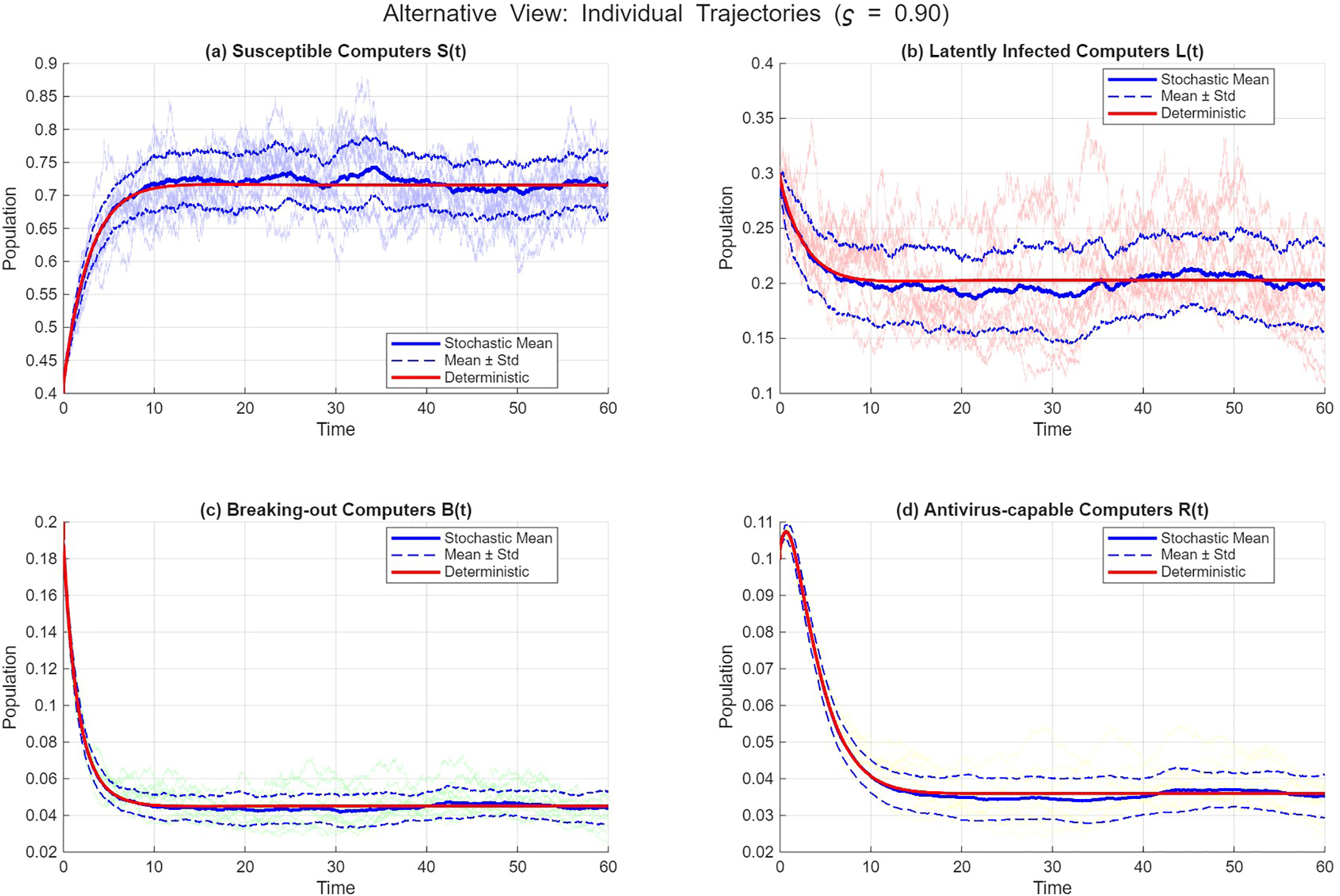
Figure 6: Multiple realizations of the stochastic Caputo-Fabrizio model showing trajectory variability. Each subplot displays 10 sample paths for (a)
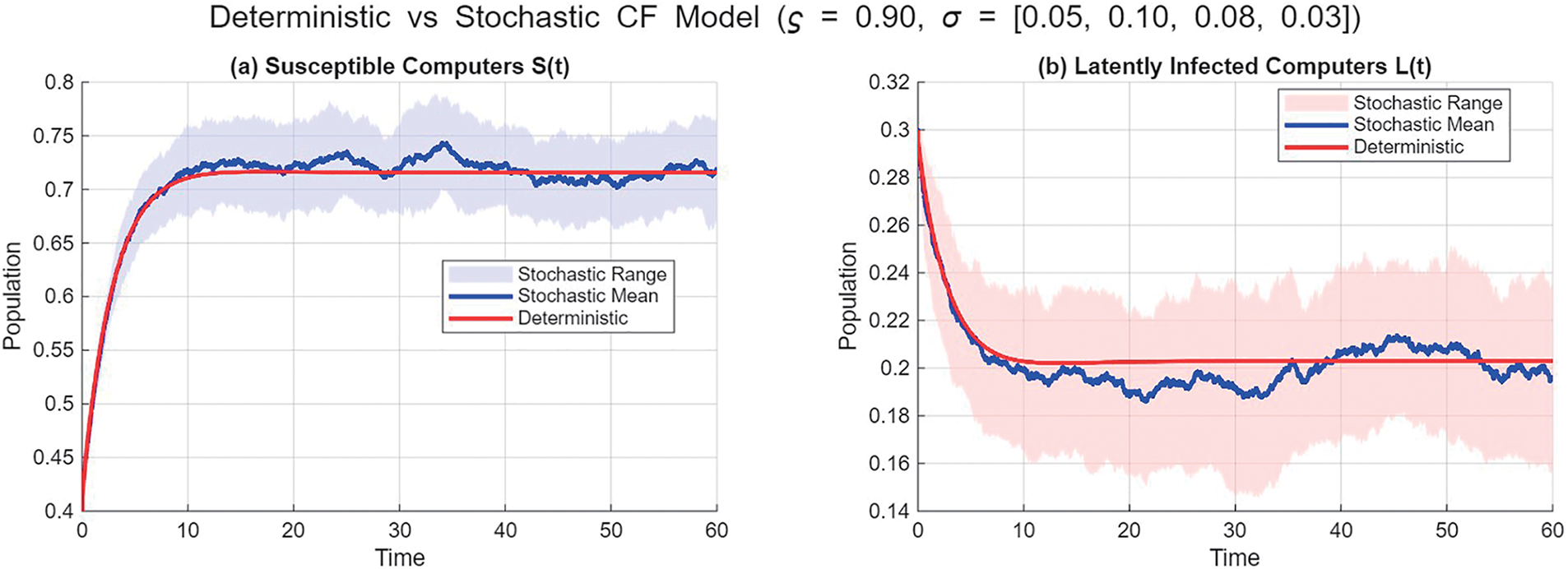
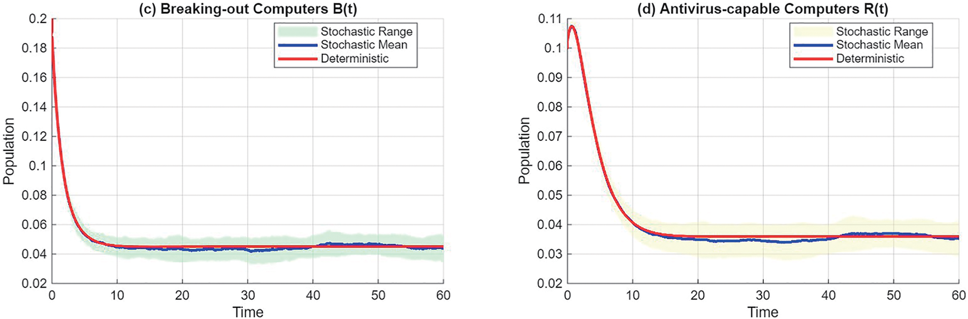
Figure 7: Comparison between deterministic trajectory (solid line) and stochastic realizations (dashed lines) for the breaking-out compartment
The stochastic framework enables:
• Probabilistic Risk Assessment: Compute
• Extreme Event Analysis: Estimate likelihood of large outbreaks via Monte Carlo simulation
• Robust Control Design: Test antivirus strategies under uncertainty to ensure effectiveness across stochastic scenarios
• Quantitative Security Metrics: Derive statistics (mean time to containment, outbreak duration distribution) for cybersecurity policy
This expanded framework provides a rigorous, implementable stochastic extension of the deterministic CF model, enhancing its realism and applicability to uncertain cyber environments where random fluctuations significantly impact virus propagation dynamics.
4.3 Derivation of the Stochastic Two-Step Adams-Bashforth Scheme
To numerically solve the stochastic system (10), we develop a two-step Adams-Bashforth-type scheme adapted for the CF derivative. We begin by applying the CF fractional integral operator to both sides of the SFDE for a generic compartment
Discretizing at time
where A and B are the same coefficients as in the deterministic scheme, and
The double stochastic integral
Substituting this approximation into the outer integral yields:
Using this approximation and simplifying, we arrive at the final Stochastic Caputo-Fabrizio Adams-Bashforth (SCF-AB) Scheme:
where
Approximating
This approximation maintains consistency with the overall numerical scheme and is standard in the context of stochastic numerical integration [24].
4.4 Implications and Expected Behavior
The introduction of stochasticity renders the model more realistic and its analysis more robust. We can anticipate several key behaviors:
1. Trajectory Variability: Unlike the deterministic model, each simulation run will produce a different path, representing one possible realization of the virus outbreak under random influences.
2. Noise-Induced Transitions: Even for parameter values that yield a virus-free equilibrium in the deterministic case, strong stochastic fluctuations (
3. Probabilistic Control Assessment: The effectiveness of antivirus measures (controlled by
This stochastic extension provides a powerful tool for risk assessment in cybersecurity, allowing analysts to simulate an ensemble of possible scenarios, quantify the likelihood of extreme events, and prepare for worst-case outcomes influenced by random network events.
Finally, Figs. 6–8 are positioned in the stochastic modeling section, depicting noise effects, trajectory variability, and noise-induced transitions. This reorganization ensures a logical and consecutive flow of visual references from Figs. 1–8.
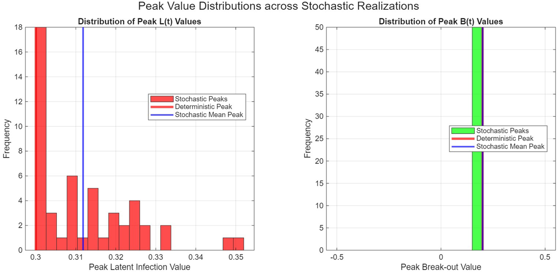
Figure 8: Schematic diagram illustrating the impact of stochastic noise on system dynamics, comparing deterministic equilibrium behavior with potential noise-induced transitions in the presence of random fluctuations.
Using the Caputo-Fabrizio (CF) derivative and its non-singular exponential memory kernel, the study introduces a new fractional-order model for the analysis of computer virus propagation and control dynamics. According to the model, the computer population is divided into four interconnected compartments: susceptible (S(t)), latently infected (L(
Under Lipschitz continuity and boundedness conditions, the theoretical foundation of our model was established through fixed-point theory. The mathematical framework ensures the model’s well-posedness and establishes a strong foundation for its numerical implementation. With a two-step Adams-Bashforth scheme tailored to the CF framework, a notable computational improvement has been achieved, with analyses of convergence and stability verifying that second-order accuracy can be achieved under suitable conditions of step sizes and smoothness.
As a result of our numerical simulations, we were able to gain valuable insight into the influence of memory effects on cyber-epidemiological dynamics. The fractional order
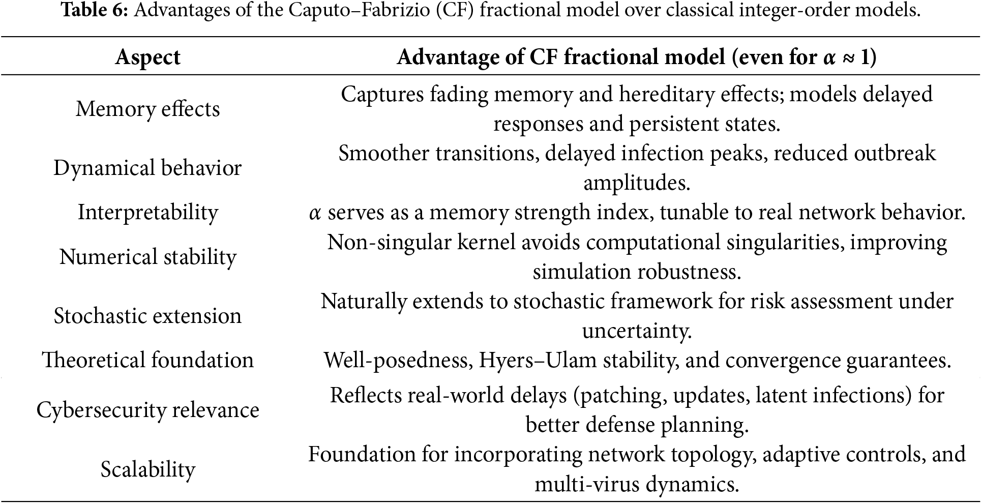
Comparing classical integer-order models with other fractional formulations (Caputo and Atangana-Baleanu) highlighted the distinct advantages of the CF approach. As a result of the non-singular kernel’s ability to accurately represent fading memory effects while avoiding computational singularities, it is particularly suitable for modelling digital environments in which instantaneous state changes are unlikely to occur.
By incorporating random fluctuations typical of real-world networks, the Stochastic Caputo-Fabrizio Adams-Bashforth (SCF-AB) scheme significantly improved the model’s applicability. The stochastic formulation facilitates probabilistic risk assessment and addresses uncertainties related to user behavior, network failures, and antivirus effectiveness. Based on this approach, key characteristics are captured, such as variability and noise-induced transitions, as illustrated in the figures shown in Figs. 6 and 7.
Sensitivity analysis, as summarised in Table 5, identified critical parameters affecting virus dynamics. There was a significant positive effect on the transmission rate (
Based on the delayed dynamics shown in Fig. 2, memory-aware models are more accurate at predicting infection persistence and outbreak timing. Observed delayed response patterns under strong memory effects indicate the need for proactive defence strategies rather than reactive ones. The use of fractional-order dynamics can improve the scheduling of antivirus updates and digital immunization initiatives. As a result of the stochastic extension (Fig. 8), it is possible to assess quantitative risks for extreme outbreak scenarios under uncertain circumstances.
With this CF-based framework, future research will be able to encompass network topology effects, time-delayed interactions, multi-virus scenarios, and adaptive control strategies. In addition to offering theoretical insights and practical tools for the development of resilient digital defense systems, the synergy between fractional calculus and computer virus modelling offers new opportunities for computational epidemiology and cybersecurity analytics.
The aim of this study is to develop a mathematical framework that utilizes Caputo-Fabrizio fractional calculus to analyze the propagation of computer viruses. This model accurately represents the dynamics of four key compartments: susceptible, latently infected, breaking-out, and antivirus-capable computers, while integrating memory effects via a non-singular exponential kernel. Using fixed-point theory, the theoretical foundations ensure the existence and uniqueness of solutions, supporting the mathematical validity of the model and its practical application.
For the CF operator, a two-step Adams-Bashforth numerical scheme represents an important computational advancement. The proposed scheme exhibits stable performance and second-order convergence, which allows for precise simulation of complex cyber-epidemiological dynamics. Based on numerical investigations, fractional-order memory has a significant impact on system behavior. It has been shown that lower values of
Comparing classical integer-order models with alternative fractional formulations underscores the unique benefits of the CF approach, especially its ability to represent fading memory effects without encountering computational singularities. Incorporating a stochastic framework via the Stochastic Caputo-Fabrizio Adams-Bashforth scheme improves the model’s applicability by addressing the inherent uncertainty associated with real-world network environments, including unpredictable user behavior and random system failures.
These findings have implications for cybersecurity practice, suggesting that memory-aware models can be used to improve outbreak prediction accuracy and guide the development of more robust defence strategies. Based on the established correlation between fractional order and system stability, antivirus deployment schedules and digital immunization initiatives may be enhanced, resulting in better allocation of cybersecurity resources.
Based on the results of this study, a strong analytical and computational basis can be established for future research in the fields of computational epidemiology and cybersecurity. The integration of fractional calculus with computer virus modelling presents opportunities to develop adaptive and predictive cybersecurity systems that accurately represent the complex dynamics of real-world digital environments, thus enhancing defence mechanisms against evolving cyber threats.
Acknowledgement: This work was supported and funded by the Deanship of Scientific Research at Imam Mohammad Ibn Saud Islamic University (IMSIU) (grant number IMSIU-DDRSP2601).
Funding Statement: This work was supported and funded by the Deanship of Scientific Research at Imam Mohammad Ibn Saud Islamic University (IMSIU) (grant number IMSIU-DDRSP2601).
Author Contributions: All authors have contributed significantly to this work. Najat Almutairi: Conceptualization, methodology, formal analysis, writing—original draft. Mohammed Messaoudi: Supervision, validation, writing—review & editing. Faisal Muteb K. Almalki: Software, visualization, data curation. Sayed Saber: Investigation, resources, writing—review & editing, project administration. All authors reviewed and approved the final version of the manuscript.
Availability of Data and Materials: The data and codes used in this study are available from the corresponding author upon reasonable request. No new experimental data were generated; all simulations are based on the mathematical model described.
Ethics Approval: Not applicable.
Conflicts of Interest: The authors declare no conflicts of interest.
References
1. Podlubny I. Fractional differential equations. San Diego, CA, USA: Academic Press; 1999. [Google Scholar]
2. Kilbas AA, Srivastava H, Trujillo J. Theory and applications of fractional differential equations. In: North holland mathematical studies. Vol. 204. Amsterdam, The Netherlands: Elsevier; 2006. doi:10.1016/S0304-0208(06)80001-0. [Google Scholar] [CrossRef]
3. Mainardi F. Fractional calculus and waves in linear viscoelasticity: an introduction to mathematical models. London, UK: Imperial College Press; 2010. doi:10.1142/9781848163300. [Google Scholar] [CrossRef]
4. Magin R. Fractional calculus models of complex dynamics in biological tissues. Comput Math Appl. 2010;59(5):1586–93. doi:10.1016/j.camwa.2009.08.039. [Google Scholar] [CrossRef]
5. Caputo M. Linear models of dissipation whose Q is almost frequency independent II. Geophys J Royal Astron Soc. 1967;13:529–39. doi:10.1111/j.1365-246X.1967.tb02303.x. [Google Scholar] [CrossRef]
6. Caputo M, Fabrizio M. A new definition of fractional derivative without singular kernel. Prog Fract Differ Appl. 2015;1(2):73–85. doi:10.3390/computation8020049. [Google Scholar] [CrossRef]
7. Losada J, Nieto JJ. Properties of a new fractional derivative without singular kernel. Prog Fract Differ Appl. 2015;1(2):87–92. [Google Scholar]
8. Liu Z, Yang X, Yang L. A fractional computer virus propagation model with saturation effect. Fractal Fract. 2025;9:587. doi:10.3390/fractalfract9090587. [Google Scholar] [CrossRef]
9. Baleanu D, Diethelm K, Scalas E, Trujillo JJ. Fractional calculus models and numerical methods. Boston, MA, USA: World Scientific; 2012. doi:10.1142/9789814355216. [Google Scholar] [CrossRef]
10. Atangana A. Fractal-fractional differentiation and integration: connecting fractal calculus and fractional calculus to predict complex system. Chaos Solitons Fractals. 2017;102(5):396–406. doi:10.1016/j.chaos.2017.04.027. [Google Scholar] [CrossRef]
11. Alsulami A, Alharb R, Albogami T, Eljaneid N, Adam H, Saber S. Controlled chaos of a fractal-fractional Newton-Leipnik system. Therm Sci. 2024;28(6):5153–60. doi:10.2298/TSCI2406153A. [Google Scholar] [CrossRef]
12. Yan T, Alhazmi M, Youssif MY, Elhag AE, Aljohani AF, Saber S. Analysis of a lorenz model using adomian decomposition and fractal-fractional operators. Therm Sci. 2024;28(6):5001–9. doi:10.2298/TSCI2406001Y. [Google Scholar] [CrossRef]
13. Alhazmi M, Dawalbait FM, Aljohani A, Taha KO, Adame HDS, Saber S. Numerical approximation method and chaos for a chaotic system in sense of Caputo-Fabrizio operator. Therm Sci. 2024;28(6):5161–8. doi:10.2298/TSCI2406161A. [Google Scholar] [CrossRef]
14. Ayaz A, Rehamn MAU, Rafiq M, Iqbal Z, Ahmed N, Akgül A, et al. Stochastic fractional order model for the computational analysis of computer virus. Sci Rep. 2025;15:33951. doi:10.1038/s41598-025-10330-5. [Google Scholar] [PubMed] [CrossRef]
15. Lefebvre M. A stochastic model for computer virus propagation. J Dyn Game. 2020;7(2):163–74. doi:10.3934/jdg.2020010. [Google Scholar] [CrossRef]
16. Saber S, Alahmari AA. Existence, stability, and control of glucose-insulin dynamics via Caputo-Fabrizio fractal-fractional operators. MethodsX. 2026;16:103757. doi:10.1016/j.mex.2025.103757. [Google Scholar] [PubMed] [CrossRef]
17. Althubyani M, Taha NE, Taha KO, Alharb RA, Saber S. Epidemiological modeling of pneumococcal pneumonia: insights from ABC fractal-fractional derivatives. Comput Model Eng Sci. 2025;143(3):3491–521. doi:10.32604/cmes.2025.061640. [Google Scholar] [CrossRef]
18. Saber S, Mirgani S. Analyzing fractional glucose-insulin dynamics using Laplace residual power series methods via the Caputo operator: stability and chaotic behavior. Beni Suef Univ J Basic Appl Sci. 2025;14(1):28. doi:10.1186/s43088-025-00608-y. [Google Scholar] [CrossRef]
19. Saber S, Dridi B, Alahmari A, Messaoudi M. Application of jumarie-stancu collocation series method and multi-step generalized differential transform method to fractional glucose-insulin. Int J Optim Control Theor Appl. 2025;15(3):464–82. doi:10.36922/IJOCTA025120054. [Google Scholar] [CrossRef]
20. Saber S, Dridi B, Alahmari A, Messaoudi M. Hyers-Ulam stability and control of fractional glucose-insulin systems. Eur J Pure Appl Math. 2025;18(2):6152. doi:10.29020/nybg.ejpam.v18i2.6152. [Google Scholar] [CrossRef]
21. Alhazmi Muflih, Mirgani SM, Aljohani AF, Saber S. Numerical simulation of a fractional glucose-insulin model via successive approximation and ABM schemes. AIMS Math. 2025;10(10):22817–49. doi:10.3934/math.20251014. [Google Scholar] [CrossRef]
22. Atangana A, Qureshi S. Modeling attractors of chaotic dynamical systems with fractal-fractional operators. Chaos Solitons Fractals. 2019;123(3):320–37. doi:10.1016/j.chaos.2019.04.020. [Google Scholar] [CrossRef]
23. Owolabi KM, Atangana A, Akgul A. Modelling and analysis of fractal-fractional partial differential equations: application to reaction-diffusion model. Alex Eng J. 2020;59(4):2477–90. doi:10.1016/j.aej.2020.03.022. [Google Scholar] [CrossRef]
24. Owolabi K, Atangana A. Numerical methods for fractional differentiation. Singapore: Springer; 2019. doi:10.1007/978-981-15-0098-5. [Google Scholar] [CrossRef]
25. Atangana A, Araz S. New numerical scheme with newton polynomial: theory, methods, and applications. Amsterdam, The Netherlands: Elsevier; 2021. p. 1–444. doi:10.1016/C2020-0-02711-8. [Google Scholar] [CrossRef]
26. Yang LX, Yang X, Zhu Q, Wen L. A computer virus model with graded cure rates. Nonlinear Anal Real World Appl. 2013;14(1):414–22. doi:10.1016/j.nonrwa.2012.07.005. [Google Scholar] [CrossRef]
27. Mishra BK, Pandey SK. Dynamic model of worms with vertical transmission in computer network. Appl Math Comput. 2011;217(21):8438–46. doi:10.1016/j.amc.2011.03.041. [Google Scholar] [CrossRef]
28. Deng W, Li C, Li J. Stability analysis of linear fractional differential system with multiple time delays. Nonlinear Dyn. 2007;48(4):409–16. doi:10.1007/s11071-006-9094-0. [Google Scholar] [CrossRef]
29. Gómez JF, Torres L, Escobar RF. Fractional derivatives with mittag-leffler kernel: trends and applications in science and engineering. Cham, Switzerland: Springer International Publishing; 2019. [Google Scholar]
30. Miura H, Kimura T, Hirata K. Modeling of malware propagation in wireless mobile networks with hotspots considering the movement of mobile clients based on cosine similarity. Electronics. 2025;14:3528. doi:10.3390/electronics14173528. [Google Scholar] [CrossRef]
31. Zhou Y, Liu BT, Zhou K, Shen SF. Malware propagation model of fractional order, optimal control strategy and simulations. Front Phys. 2023;11:1201053. doi:10.3389/fphy.2023.1201053. [Google Scholar] [CrossRef]
32. Zhang Z, Yang H. Hopf bifurcation of an SIQR computer virus model with time delay. Discret Dyn Nat Soc. 2015;2015:101874. doi:10.1155/2015/101874. [Google Scholar] [CrossRef]
33. Raza A, Fatima U, Rafiq M, Ahmed N, Khan I, Nisar KS, et al. Mathematical analysis and design of the nonstandard computational method for an epidemic model of computer virus with delay effect: application of mathematical biology in computer science. Results Phys. 2020;21:103750. doi:10.1016/j.rinp.2020.103750. [Google Scholar] [CrossRef]
34. Ahmed KIA, Mirgani SM, Seadawy A, Saber S. A comprehensive investigation of fractional glucose-insulin dynamics: existence, stability, and numerical comparisons using residual power series and generalized Runge-Kutta methods. J Taibah Univ Sci. 2025;19(1):2460280. doi:10.1080/16583655.2025.2460280. [Google Scholar] [CrossRef]
35. Qabaja M, Asad J, Wannan R. Chaotic model for development of HIV virus. In: Mathematical modeling in physical sciences (ICMSQUARE 2023). Cham, Switzerland: Springer; 2024. p. 555–69. doi:10.1007/978-3-031-52965-8_43. [Google Scholar] [CrossRef]
36. Gan C, Yang X, Liu W, Zhu Q, Zhang X. An epidemic model of computer viruses with vaccination and generalized nonlinear incidence rate. Appl Math Comput. 2013;222(1):265–74. doi:10.1016/j.amc.2013.07.055. [Google Scholar] [CrossRef]
37. Attia N, Akgül A, Seba D, Nour A, Asad J. A novel method for fractal-fractional differential equations. Alex Eng J. 2022;61(12):9733–48. doi:10.1016/j.aej.2022.02.004. [Google Scholar] [CrossRef]
38. Murthy BSN, Srinivas MN, Madhusudanan V, Zeb A, Tag-Eldin EM, Etemad S, et al. The impact of Caputo-Fabrizio fractional derivative and the dynamics of noise on worm propagation in wireless IoT networks. Alex Eng J. 2024;91(9):558–79. doi:10.1016/j.aej.2024.02.027. [Google Scholar] [CrossRef]
39. Pastor-Satorras R, Castellano C, Van Mieghem P, Vespignani A. Epidemic processes in complex networks. Rev Mod Phys. 2015;87(3):925–79. doi:10.1103/RevModPhys.87.925. [Google Scholar] [CrossRef]
40. Wang Y, Chakrabarti D, Wang C, Faloutsos C. Epidemic spreading in real networks: an eigenvalue viewpoint. In: Proceedings of the 22nd International Symposium on Reliable Distributed Systems; 2003 Oct 6–8; Florence, Italy. p. 25–34. doi:10.1109/RELDIS.2003.1238052. [Google Scholar] [CrossRef]
41. Althubyani M, Saber S. Hyers-Ulam stability of fractal-fractional computer virus models with the Atangana-Baleanu operator. Fractal Fract. 2025;9:158. doi:10.3390/fractalfract9030158. [Google Scholar] [CrossRef]
42. Zhang J, Feng H, Liu B, Zhao D. Survey of technology in network security situation awareness. Sensors. 2023;23(5):2608. doi:10.3390/s23052608. [Google Scholar] [PubMed] [CrossRef]
43. Dang QA, Hoang MT. Positivity and global stability preserving NSFD schemes for a mixing propagation model of computer viruses. J Comput Appl Math. 2020;374:112753. doi:10.1016/j.cam.2020.112753. [Google Scholar] [CrossRef]
44. Wacker B. Qualitative study of a dynamical system for computer virus propagation—a nonstandard finite-difference-methodological view. Math Methods Appl Sci. 2025;48(8):9272–91. doi:10.1002/mma.10798. [Google Scholar] [CrossRef]
45. Ahmad I, Abu Bakar A, Ahmad H, Khan A, Abdeljawad T. Investigating virus spread analysis in computer networks with atangana-baleanu fractional derivative models. Fractals. 2024;32(07n08):2440043. doi:10.1142/S0218348X24400437. [Google Scholar] [CrossRef]
46. Ahmad I, Bakar AA, Jan R, Yussof S. Dynamic behaviors of a modified computer virus model: insights into parameters and network attributes. Alex Eng J. 2024;103(7):266–77. doi:10.1016/j.aej.2024.06.009. [Google Scholar] [CrossRef]
47. Li Y, Chen YQ, Podlubny I. Stability of fractional-order nonlinear dynamic systems: lyapunov direct method and generalized Mittag-Leffler stability. Comput Math Appl. 2010;59(5):1810–21. doi:10.1016/j.camwa.2009.08.019. [Google Scholar] [CrossRef]
48. Agarwal RP, de Andrade B, Siracusa G. On fractional integro-differential equations with state-dependent delay. Comput Math Appl. 2011;62(3):1143–9. doi:10.1016/j.camwa.2011.02.033. [Google Scholar] [CrossRef]
Cite This Article
 Copyright © 2026 The Author(s). Published by Tech Science Press.
This work is licensed under a Creative Commons Attribution 4.0 International License , which permits unrestricted use, distribution, and reproduction in any medium, provided the original work is properly cited.
 Downloads
 Citation Tools