An Interpretable AI Framework for Predicting Groundwater Contamination under Atmospheric and Industrial Pollution Using Metaheuristic-Optimized Deep Learning

1  Introduction

Groundwater is a critical freshwater resource for drinking, agriculture, and industrial use, particularly in densely populated and rapidly developing regions. However, increasing industrial activities, urban expansion, agricultural intensification, and atmospheric deposition have significantly degraded groundwater quality worldwide, posing serious risks to ecosystems and public health [1,2]. The systems of groundwater are particularly susceptible in South Asian areas such as Bangladesh where groundwater aquifers are shallow, monsoons have a high recharge rate, and regulatory measures are absent [3,4].

The use of data based methods to model and predict groundwater quality has been used in recent studies because of the capability to deal with non linear relationships between a number of hydrochemical parameters. Groundwater quality assessment has been extensively reported to rely on traditional statistical models and machine learning techniques, including multiple linear regression [5], the support vector machines [6], the random forests [7], and the artificial neural networks [8]. Although these models have reasonable predictive performance, their models are often limited by shallow feature representations and low-capacity to model complex spatial-temporal dependencies [9].

DL models have received growing interest in groundwater and environmental applications in order to overcome such challenges. CNNs and LSTM networks have been utilized in predicting ground water level and quality with better accuracy using their temporal pattern and local feature extraction [10–12]. Recently, it has become possible to suggest hybrid and optimization-aided deep learning models to improve the convergence speed, feature selection, and robustness [13,14]. However, most of the available literature is based on black-box structures and little interpretable and also fails to address the interplay between atmospheric deposition and industrial pollution on groundwater systems.

Although there has been significant advancement, the current literature has some gaps. To begin with, the majority of the groundwater quality forecasting research addresses the individual pollution sources, failing to explicitly include the atmospheric and industrial impacts in a single modeling system [15,16]. Second, traditional deep learning models may not be interpretable enough to be used practically in making environmental decisions [17]. Third, most of the studies use fixed sets of features without optimization of the adaptability of the feature set, which can potentially decrease the generalization ability when used in heterogeneous hydrogeological systems [18]. But the models based on ANN suffer from some serious drawbacks like overfitting and generalization capability, which demands a large amount of data. However, they still have the disadvantage of being black boxes since they do not explain how each input variable affects the output prediction [19,20].

Therefore, the present study is focused on the development of an interpretable and explainable AI model for the prediction of groundwater quality. Such an interpretative model will not only contribute to an increase in accuracy but also lead to ensuring interpretability and adaptability in rendering feasible solutions to real-world applications. The proposed framework includes a combination of Spatial–Temporal-Assisted Deep Belief Network (StaDBN) along with the Whale Optimization Algorithm and Tiki-Taka Algorithm (WOA–TTA), representing an advanced AI strategy for the prediction of the quality of groundwater. The StaDBN module captures complex nonlinear interactions and spatiotemporal dependencies that describe the variability of groundwater quality coming from multiple sources of pollution. Besides, its hyperparameters are optimized by the WOA-TTA component. Moreover, the interpretable model leverages an optimized feature selector based on the Addax Optimization Algorithm, AOA, which selects the most informative and influential features within the historical dataset for making the model output more interpretable.

The key findings of this research are summarized below:

•   Developed an interpretable AI model for accurate prediction of groundwater quality influenced by multiple pollution sources using metaheuristic optimization and deep learning.

•   Proposed an optimized feature selection method leveraging the efficiency of the Addax Optimization Algorithm to identify and select the most relevant attributes influencing GQI.

•   Designed a hybrid predictive model by integrating StaDBN with WOA and TTA to learn complex hierarchical feature representations and predict GQI effectively.

•   Implemented the model in Python and evaluated its performance using standard statistical metrics including root mean square error (RMSE), Nash–Sutcliffe efficiency (NSE), mean absolute error (MAE), and correlation coefficient (R).

The organization of the enduring sections of the article are described as follows: Section 2 presents detailed review of recent research works related to the presented work, Section 3 illustrates the study location, Section 4 details the working of the designed methodology, Section 5 analyzes the results and discussion, and Section 6 describes the research conclusion.

2  Related Works

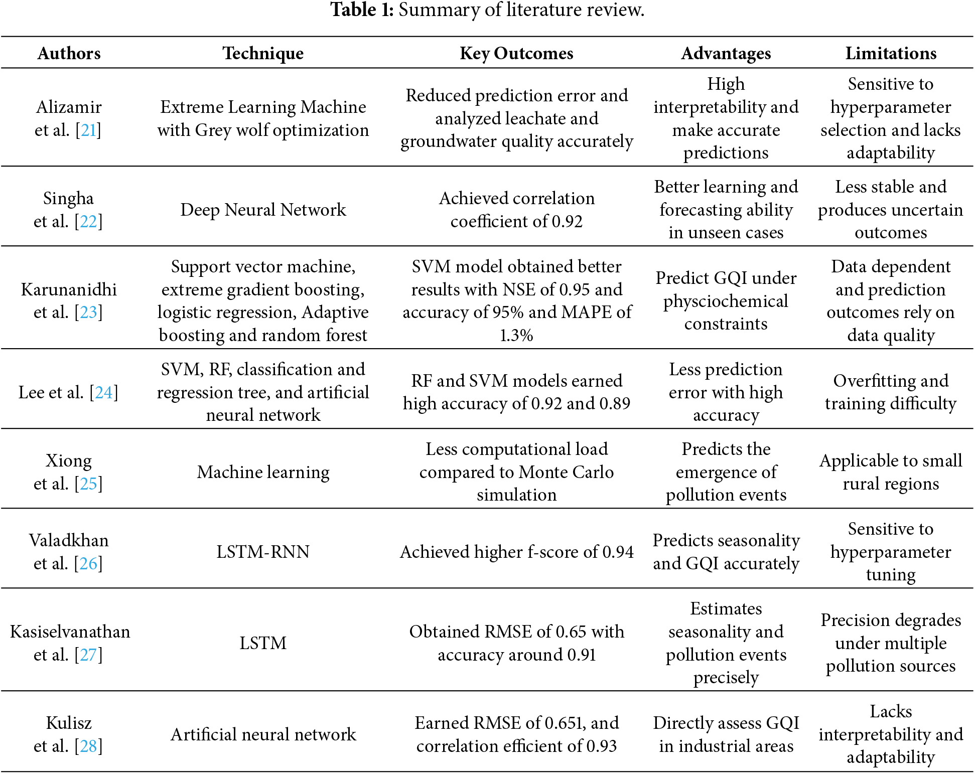
Several recent investigations have explored the use of data-driven and AI-based models for groundwater quality prediction, as summarized below. These studies have employed a range of hybrid optimization and deep learning techniques to enhance prediction accuracy and interpretability. For instance, Alizamir et al. [21] proposed a hybrid AI-based approach for forecasting landfill leachate and groundwater quality. The model was an integration of a method with a Grey Wolf Optimizer and an Extreme Learning Machine to improve the predictive performance. The sample of groundwater and leachate were taken in Iran and the effectiveness of the model was evaluated against four already existing algorithms. The comparative test proved that the method had lower error rates than traditional models and thus it is a strong framework in the analysis of leachate and ground water quality. Nevertheless, tuning of hyperparameters and lack of flexibility to solve the different input conditions are sensitive to this approach.

Singha et al. [22] created a deep learning system to predict the groundwater quality. The experiment assessed the results of Deep Neural Network (DNN) model and contrasted it with the already existing algorithms, such as ANN, Extreme Gradient Boosting (XGBoost), and RF. The training and validation were based on the data of the Raipur district, Chhattisgarh (India). DNN model showed the highest correlation coefficient of 0.96 which is better than ANN, XGBoost and RF (0.90, 0.89, and 0.88, respectively). Nevertheless, the DNN was unstable when it comes to making predictions, which made it less applicable in the real-world scenario.

Karunanidhi et al. [23] suggested a machine learning-based prediction model to measure groundwater quality. It was an attempt to use parameters of sodium, fluoride and calcium to predict and track the Index of Groundwater Quality (GQI). The five ML methods, which included Support Vector Machine (SVM), Extreme Gradient Boosting, Logistic Regression, Adaptive Boosting, and Random Forest were applied to Arjunanadi, Tamil Nadu data. Amongst them, SVM gave the best results, with a Mean Absolute Percentage Error (MAPE) of 1.3, NSE of 0.95 and accuracy of 95. However, these models are data-dependent and their functioning is affected by the quality of data.

Lee et al. [24] developed a smart model to forecast nitrate inflow in groundwater based on machine learning algorithms. The experiment used 183 groundwater samples and was taken out of different wells in South Korea and tested four models: SVM, RF, Classification and Regression Tree (CART), and ANN. The findings showed that RF and SVM had greater predictions with low errors of ground water parameters. Nevertheless, such models are likely to be overfitted and cannot be used to predict long-term trends.

Xiong et al. [25] developed a groundwater pollution monitoring system to identify the occurrences of pollution and facilitate prompt control action. The study sought to fill the shortcomings of the Monte Carlo Simulation method of prediction of GQI by utilizing machine learning method. The collection was done at a domestic landfill in the city of Baicheng, China. As it was demonstrated, the proposed ML-based strategy could perform better in comparison with the simulation method that had less computational cost, but was limited to small rural areas.

Valadkhan et al. [26] created a smart algorithm of determining the ground water quality to avoid polluting water. In Damavand, Iran, five locations of groundwater samples were sampled and the sample was taken across 2009–2021. The model was based on a Long Short-Term Memory (LSTM) architecture to make predictions and attained an F-score of 0.94. The training process was however very complicated and a very sensitive area in regard to hyperparameter settings.

Kasiselvanathan et al. [27] used an LSTM-based neural network to assess GQI and solve water quality problems in western Tamil Nadu. Based on the data obtained in the southern areas of the Tamil Nadu, the model was effective in capturing the variation in the season and trends that are related to the pollution of groundwater. However, it could not predict GQI accurately under multiple pollution sources, which is essential for real-world implementation.

Kulisz et al. [28] proposed an ANN-based prediction framework to forecast and monitor groundwater quality by analyzing physicochemical parameters. Groundwater data were collected from 19 wells located near shale gas extraction sites in Lublin, eastern Poland. The model achieved an RMSE of 0.651 and a correlation coefficient of 0.93, demonstrating its applicability for groundwater quality assessment in industrial regions. However, this approach lacked interpretability and adaptability. A comparative summary of the reviewed studies, including their techniques, advantages, and limitations, is presented in Table 1.

Although several ML and DL approaches have been explored for groundwater quality prediction, most existing studies rely on conventional models such as support vector machines, random forests, decision trees, and ANN. While these models provide reasonable performance, recent advances in deep learning particularly attention-based architectures, transformer models, and generative adversarial network (GAN)-based data augmentation techniques—have demonstrated strong predictive capability in related domains such as anomaly and fault detection, time-series forecasting, and complex environmental monitoring applications. These advanced models are effective in capturing long-range dependencies, contextual relationships, and data scarcity challenges, which may further enhance groundwater quality prediction performance.

The present study focuses on developing an interpretable and computationally efficient framework by integrating a StaDBN with metaheuristic optimization. However, the drawback in the presented work is that the study does not incorporate a comparative analysis regarding the recent attention-driven models or transformer models of deep learning. Moreover, the use of GAN models, which can be a solution for the problem of the unavailability of sufficient samples, is not taken into consideration. These applications have been determined to be the future research path to test the robustness and efficiency of the models. Motivated by the above gaps, this study makes the following key contributions:

•   A Spatial–Temporal-Assisted Deep Belief Network (StaDBN) model is introduced to effectively capture the spatial relationships among monitoring wells as well as the temporal changes of groundwater quality.

•   In the proposed methodology, the Addax Optimization Algorithm is used for adaptive feature selection. This aims at enhancing the robustness of the model as well as eliminating redundancy.

•   A Whale Optimization Algorithm with Test-Time Augmentation (WOA-TTA) is implemented for efficient hyperparameter optimization.

•   It should be noted that the framework is tested for the joint effects of atmospheric and industrial pollution, giving a more realistic evaluation of the quality of the groundwater.

•   The proposed algorithm is made more interpretable and reproducible, which makes its practical application feasible.

•   Conducted comprehensive comparative evaluation against conventional machine learning models (e.g., ANN, SVM, Random Forest) and baseline deep learning methods (e.g., LSTM), demonstrating higher correlation, improved NSE, and lower MAE and RMSE, thus validating the superior performance of the proposed framework.

Through these contributions, the proposed approach advances the state of the art in groundwater quality prediction by addressing key methodological and application-level limitations identified in previous studies.

Problem Statement

Paper Although the application of ML and deep learning (DL) models has revolutionized the assessment of groundwater quality, there are some challenges that are still unaddressed. Most of the existing models show high performance in terms of accuracy on the given datasets, but they are sensitive to hyperparameters, prone to overfitting, and not flexible enough to handle various and changing groundwater conditions caused by multiple pollution sources. Furthermore, these conventional models function as black-box models, making them less explainable and interpretable. The situation presents a difficulty in the course of monitoring the environment and making policies based on it. Furthermore, the present models could not recognize spatiotemporal dependencies which are significant for the evaluation of the impact of different pollution sources as well as hydrogeological and human-made conditions on the quality of groundwater prediction. Such difficulties bring forth the necessity for a smart system that is capable of handling the intricate and high-dimensional groundwater data that constantly changes and is also strong, clear, and widely applicable [21–28].

3  Study Location

The study domain that covers the Rooppur Nuclear Power Plant (RNPP) area is located in Ishwardi, the westernmost Upazila of Pabna District under Bangladesh’s Rajshahi Division. It is positioned between latitudes of 24°03′ N and 24°15′ N, and longitudes of 89°00′ E and 89°11′ E and occupies an area of about 246.90 km2. The region is characterized by a humid subtropical climate, with pronounced wet and dry seasons that significantly influence groundwater recharge, contaminant transport, and pollutant dispersion processes. The surface deposits found in this area are considered to be part of the Ganges River Floodplain, which was formed mainly by the rivers Ganges and Jamuna through fluvial processes. Besides, the area mainly consists of alluvial sand and estuarine deposits to its geological identity [29]. The terrain here is mostly flat with very few sites having slight raise and small areas of depression. Therefore, lowlands in the region act as rainwater catchments, which in turn supply water to the Padma River and other nearby streams, beels, canals, and ponds. Only after overland runoff or vertical infiltration into the subsurface has occurred do this water bodies drain away and dry up.

The study area has been selected due to the coexistence of industrial activities and atmospheric deposition sources that can potentially affect groundwater quality. The RNPP represents a major industrial infrastructure in the region, accompanied by construction activities, increased vehicular movement, material storage, and auxiliary industrial operations, all of which may contribute trace metals and chemical residues to the surrounding environment. In addition, nearby residential settlements and agricultural practices further introduce anthropogenic stressors such as domestic effluents and fertilizer-derived contaminants.

The weather conditions in the region including atmospheric pollution are significant because of the seasonal rainfall patterns in the area that increase wet deposition of airborne particulates and ease leaching of contaminants into the underground. Monsoon atmospheric deposition, along with surface runoff, makes potentially toxic elements more mobile and allows their movement into shallow alluvial aquifers typical of the Ganges River floodplain. It is these industrial and atmospheric effects that necessitate the justification of the interest of this study to groundwater quality prediction in the presence of atmospheric and industrial pollution conditions as is depicted in the title of the work.

Geologically, the region is a series of sand, silt, and clay layers of Quaternary alluvial sediments which contain superficial to moderately deep aquifers that are extremely vulnerable to surface runoff contamination. The hydrogeological environment supports the recharge of groundwater by the monsoonal rains, and allows the movement of dissolved contaminants to underground water bodies.

The climate of the area is humid subtropical with clear wet (monsoon) and dry seasons. Dense rainfall in the monsoon season has a great impact on groundwater recharge, pollution leaching, and atmospheric deposition, and dry season period is linked to low levels of dilution and high concentration of dissolved minerals.

Regarding land-use, the study area is affected by industrial activities, residential activities, and agricultural activities. The existence of the RNPP and the related infrastructure is a significant industrial source, and the anthropogenic pressures are supplemented by settlements and transportation as well as agricultural activities. All these facts precondition the fact that the region is environmentally sensitive and can serve to explore the quality of groundwater during atmospheric and industrial pollution conditions.

According to the weather data, the region with the highest air temperatures in the range 24°C–35.8°C, as well as the lowest air temperatures in the range 10°C–26°C, is the region of study. Rainfall data collected by the Bangladesh Meteorological Department in the region is 1656.2 mm in a year, with the highest in July amounting to 335.6 mm, while January is the lowest with 8.1 mm. According to the aquifer investigation, the water table depth in the research area ranges from 1.99 to 9.95 m. Because of the significant rains in May and July, the groundwater table often increases by 3 to 6 m. From August to October, however, it steadily drops because the aquifer can no longer hold more water. Groundwater resources account for approximately 94% of the water supply demand for domestic, agricultural, and industrial activities. Groundwater sampling for PTE contamination assessment involved nine water wells. Four wells (RN-W1, RN-W2, RN-W3, and RN-W4) existed within the confines of the Rooppur Nuclear Power Plant (RNPP), while the remaining wells (RA-W1, RA-W2, RA-W3, RA-W4, and RA-W5) were in the adjacent residential area of RNPP.

4  Proposed GWQP-StaDBN-WOA-TTA for Groundwater Quality Prediction

Hence a novel solution was developed in the presented study for predicting groundwater quality accurately under diverse pollution sources. The proposed framework constitutes five stages namely: (1) data collection, (2) Data preprocessing, (3) Feature selection, (4) StaDBN training and prediction and (5) Model optimization. In data collection stage, historical data containing information regarding groundwater quality of the region for the past decades. The collected data is preprocessed by following steps like missing value handling, outlier removal, and normalization in the second stage. In the third stage, an optimized feature selector was designed leveraging AOA approach to identify the most relevant and informative attributes influencing groundwater quality. These features are used for training the designed StaDBN model to predict groundwater quality under multiple pollution sources in the fourth stage. Finally, hyperparameter optimization was performed using WOA-TTA, which fine-tunes the hyperparameters to its optimal value. This combination of meta-heuristic optimization and deep learning enables us to predict groundwater quality accurately with high accuracy and less computational time. Fig. 1 presents the architecture of the developed framework.

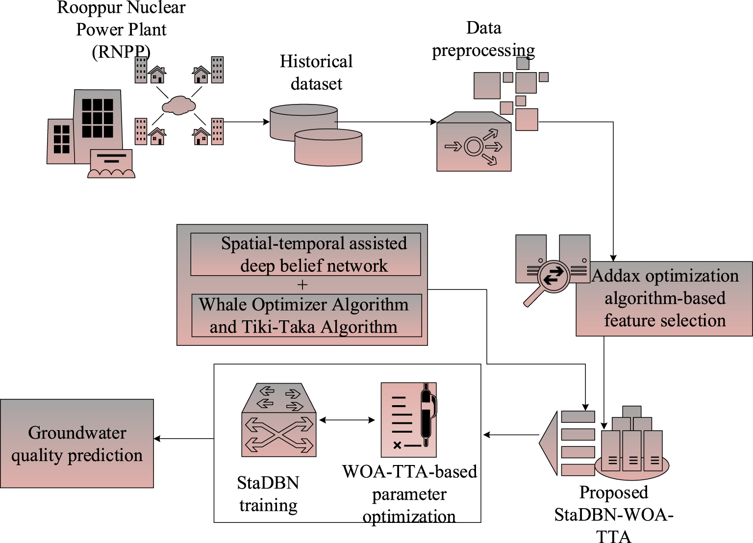
Figure 1: Proposed GWQP-StaDBN-WOA-TTA architecture.

4.1 Data Acquisition

In this section, the methodology for data acquisition concerning groundwater quality within the RNPP vicinity and its adjacent residential zone is delineated. The samples of groundwater were collected from nine monitoring wells spread over the RNPP premises and also the adjacent residential areas to capture the spatial variability in water quality. To account for temporal variations under repeated seasons of the climate regime, samples were collected during multiple seasons. For proper laboratory analysis, sampling was conducted according to standard protocols to ensure sample integrity. The geographical region considered for the study was Ishwardi Upazila, Pabna District, Bangladesh. The hydrogeology conditions under which the region stands, being a humid floodplain of the Ganges River where alluvial deposits are present in a humid subtropical climatic condition, were considered. The influence of surface water bodies on groundwater recharge as well as contaminant migration was also highlighted. Meteorological factors, including changes in temperature and annual rainfall variations, were considered as important climatic data [29]. The aquifer parameters, including water level variations, were also significant parameters.

A deliberate groundwater sampling program was conducted at nine intentionally selected well locations, including four within the operating area of the RNPP (RN W1-RN W4) and five in the nearby residential area (RA W1-RA W5). The main aim of the distribution was to identify any existing distinctions in groundwater quality influenced by both industrial and residential activities. The ground water samples were obtained in the nine monitoring wells that were analyzed in accordance with the standard procedures of assessing the water quality. Calibrated portable multiparameter probes were used to measure physicochemical parameters such as pH, temperature, electrical conductivity (EC) at the sampling sites to reduce changes of the samples due to sample transport and storage. EC was used to estimate total dissolved solids (TDS) by comparing results to standard conversion factors and total hardness (TH) was determined in the laboratory through ethylenediaminetetraacetic acid (EDTA) titrimetric processes in compliance with recommended water analysis standards.

To determine potentially toxic elements (PTEs), such as Fe, Cu, Pb, Mn, Cr, Cd, and As in the groundwater, the samples were taken in pre-cleaned polyethylene bottles and acidified with nitric acid to maintain the levels of metals. In analytical procedures that are suggested to be used in evaluation of trace metals in groundwater, the levels of these elements were measured in the laboratory with atomic absorption spectrometry (AAS) or inductively coupled plasma-based methods. The quality assurance and quality control (QA/QC) procedures such as calibration of instruments, reagent blanks, and replicate analysis were used to guarantee the accuracy and reliability of the analysis.

The dataset that was generated, including physicochemical indicators and PTE concentrations, offered a stable and good-quality input to train and test the proposed GWQP-StaDBN-WOA-TTA model, which would allow making a solid prediction of the groundwater quality with any industrial and atmospheric pollution cases.

4.2 Data Preprocessing

Preprocessing is an essential step in groundwater quality prediction. The main goal of data preprocessing is to convert raw datasets into a suitable format that can be easily processed by the ML algorithms. Generally, the raw data gathered from the public sources contains missing/null values, errors and outliers. These constraints make the data analysis process complex, resulting in increased training time and prediction errors. Here, the groundwater historical data was preprocessed by following three steps: missing value handling, outlier removal and normalization. In the missing value handling step, K-Nearest Neighbor (KNN) imputation approach was used for estimating null values present in the dataset. This algorithm estimates k nearest neighbors for a missing instance from all complete instances in the input dataset. Consequently, fill the missing data point with the most frequent one occurring in the neighbors. This approach determines Euclidean distance, a common metric in hydrological data imputation [22], for identifying the nearest neighbors and it is calculated using Eq. (1).

Ed(di,dj)=∑k=1m(dik−djk)2(1)

where Ed defines Euclidean distance, di, dj are the two data points, and m denotes the total amount of data points present in the dataset. Further, the algorithm selects the k closest complete instances and replaces the missing value. After missing value handling, the next step is outlier handling. Outliers are datapoints that significantly vary from other data points (extremely high or extremely low). Here, the interquartile (IQR) method was used for outlier detection. This is a statistical approach that detects variability in the dataset by dividing the dataset into quartiles. Initially, the dataset is sorted in ascending order and then it was divided into four equal quartiles (Q1, Q2, Q3 and Q4). Consequently, IQR was determined by subtracting Q1 from Q3 and the outliers [30] are identified by following the condition stated in Eq. (2).

Outliers={di<Q1−1.5×IQRdi>Q3+1.5×IQR(2)

Once the outliers are detected, the next step is to replace the outliers with an appropriate score with the median of the corresponding values to ensure data integrity. Finally, data normalization was performed using the z-score algorithm, following standard practices in groundwater salinity and contamination studies [15], to standardize databases and to transform all features to a common scale. Z-score is determined using Eq. (3).

z−score=di−mdstd(3)

where md denotes mean and std indicates the standard deviation. These steps not only simplify data analysis but also improve data consistency and quality.

4.3 AOA for Feature Selection

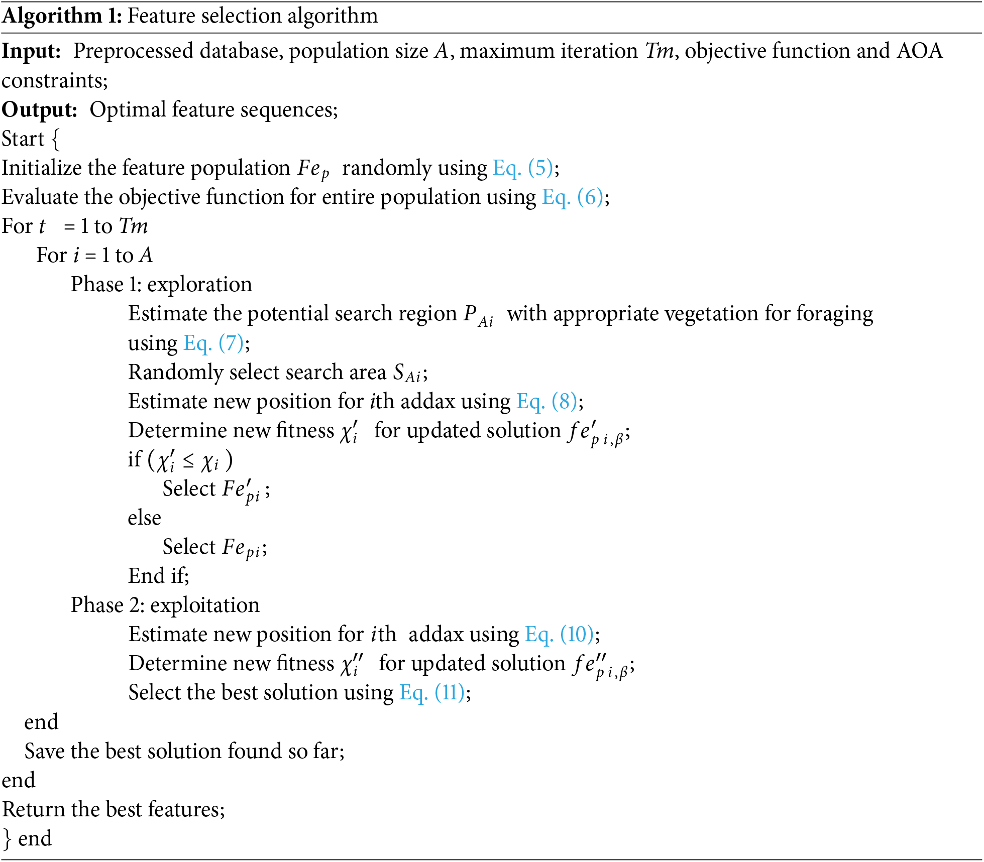
Feature selection defines the process of identifying and selecting the most relevant and significant attributes from the preprocessed database, while discarding the irrelevant ones. The main objective of this step is to reduce data dimensionality and to address interpretability issues, which are inherent in deep learning models. In the presented study, an optimized feature selector was modeled leveraging the optimization capacity of AOA technique [31]. AOA is a nature-inspired optimization model that mimics the natural characteristics of addax in nature. This algorithm follows foraging methodology and digging skills of addax to solve the optimization problem. The theoretical formulation of this approach is modeled as two phases: exploration (simulated considering the addax’s foraging behavior) and exploitation (simulated based on addax’s digging skills). The main advantage of this approach over conventional optimization techniques such as genetic algorithm (GA), particle swarm optimization (PSO), etc., is its effectiveness to provide solutions for real-world optimization problems with its greater capacity in exploration and exploitation and establishing a balance between them in its searching phase. Here, this approach was deployed for selecting the attribute with high relevance for training the prediction algorithm to forecast groundwater quality index for future cases. Since AOA is a population-based optimization algorithm, the feature selection process begins with the random initialization of addax population. Here, the Addax population indicates feature population (available features in the preprocessed database), and the best position of addax represents the feature with high relevance to GQI. The initialization process is mathematically formulated in Eqs. (4) and (5).

Fep=[Fep1⋮Fepi⋮FepA]=[fep1×1⋯fep1×β⋯fep1×B⋮⋱⋮⋱⋮fepi×1⋯fepi×β⋯fepi×B⋮⋱⋮⋱⋮fepA×1⋯fepA×β⋯fepA×B]A×B(4)

fepi×β=Lb+κ.(Ub−Lb)(5)

where Fep denotes feature population, Fepi represents the ith addax (feature subsets), fepi×β indicates βth dimension in the search space, A defines number of addax in the population, B refers to total decision variables, Lb denotes lower bound of search space, Ub represents upper bound, and κ indicates random number. After initialization, the fitness function was evaluated for each addax (feature subset) in the population based on the objective function (high relevance). The fitness of the population is defined in Eq. (6).

χ=[χ1⋮χi⋮χA]=[χ(Fep1)⋮χ(Fepi)⋮χ(FepA)]A×B(6)

where χ denotes the fitness function of the addax population. The feature subset with high relevance typically has lower fitness and vice versa. The mathematical modeling of AOA-based feature selection involves two phases: (i) exploration and (ii) exploitation.

1. Phase 1 (exploration)

In the first phase, the positions of the addax population were adjusted in the problem-solving space (search space) following its foraging behavior. Generally, the addax population feeds on shrub leaves, herbs, grasses, existing bushes and leguminous plants. They have the tendency to track rainfall and find regions with greater vegetation. Based on this characteristic, they exhibit extensive searches to identify food sources. In this searching, the positions of the addaxes are changed extensively, creating a significant shift in the position of population members. Here, each member in the population assumes the positions of other members with high objective function as appropriate foraging regions, as described in Eq. (7).

PAi={Fepk:χk<χiandk≠iwherei=1,2,3,.......,Aandk∈{1,2,3,..........,A}(7)

where PAi represents the potential search region with appropriate vegetation for foraging for the ith addax, Fepk indicates the member of the population having a higher objective function value compared to the ith addax, and χk denotes the objective function value [31]. In the foraging process, each addax selects one of the designed regions and shifts towards suitable vegetation, resulting in new position of the AOA population. This process is formulated in Eqs. (8) and (9).

fepi,β′=fepi,β+Ri,β.(SAi−Ii,β.fepi,β)(8)

Fepi={Fepi′;χi′≤χiFepi;else(9)

where fepi,β′ denotes the updated position, fepi,β represents current position, SAi indicates the selected region for foraging, Ri,β defines the random number [0, 1], and Ii,β refers to randomly selected integers [1 or 2]. After position update, the fitness was again estimated for updated position. If the estimated new fitness χi′ is less than or equal to previous fitness means, the updated solution is selected and vice versa.

2. Phase 2 (exploitation)

In this phase, the position of the Addax population is updated by following their digging skills in the problem-solving space. Typically, the addaxes dig in shady places in the daytime and rest in the produced depressions. In this phase, there will be small changes (updates) in the addax positions, creating slight variations in position of AOA population (local search). The position update in this phase is formulated in Eqs. (10) and (11).

fepi,β′′=fepi,β+(1−2Ri,β).Ubj−Lbjt(10)

Fepi={Fepi′′;χi′′≤χiFepi;else(11)

where fepi,β′′ defines the position updated in the digging stage (exploitation), χi′′ represents the fitness of the updated addax in digging process, and t denotes iteration counter. This process of position update continuous until reaching the maximum iteration count. In each iteration, the AOA algorithm returns the best positions of addax (optimal feature sequences) that is fed into the proposed DL model for groundwater quality prediction. This optimized feature selection process helps in boosting the designed StaDBN model’s training speed by allowing it to focus on important attributes influencing groundwater quality. Also, this increases the system’s interpretability by illustrating the features having greater significance in estimating groundwater quality. Algorithm 1 illustrates the designed feature selection algorithm.

4.4 Groundwater Quality Prediction Using StaDBN-WOA-TTA

To predict the groundwater quality, a novel approach was proposed in this study leveraging the efficiency of StaDBN and WOA-TTA approach. By integrating hybrid meta-heuristic optimization into a deep learning approach, this method prevents issues like limited adaptability, hyperparameter sensitivity, and false predictions.

4.4.1 Spatial-Temporal Assisted Deep Belief Network

Deep Belief Networks are a deep learning approach developed by stacking various Restricted Boltzmann Machines (RBMs) to analyze data through unsupervised learning. In the proposed StaDBN, the conventional DBN system architecture was improved to extract spatial features and temporal dependencies from historical groundwater data under multiple pollution cases across various time steps. This improvement enables the system to learn both geographical relations and evolutionary trends associated with groundwater quality in the region. The proposed StaDBN model includes five layers: input layer, hidden layer (RBMs), spatial extraction layer, temporal layer and output layer. The input layer accepts the selected feature subsets from AOA module and transforms it into an appropriate format suitable for processing in subsequent layers. The hidden layer defines stacked RBMs. RBM is a two-layer bipartisan graphic model with a sequence of invisible units Iu, a set of visible units Vu, and symmetrical interconnections defined by a weight matrix Wm between these two layers. The join probabilities of the RBM of the visible units Vu and the hidden units Hu are defined in Eq. (12).

Pj(Vu,Hu;Wm,q,o)=1PF(eξ(Vu,Hu;Wm,q,o))(12)

where ξ represents the energy function, q, o defines the model constraints and PF denotes the partition function. The partition function and the energy function are formulated in Eqs. (13) and (14).

PF=∑Vu′,Hu′eξ(Vu′,Hu′;Wm,q,o)(13)

ξ(Vu,Hu;Wm,q,o)=−H→uWmV→u−o→Hu−c→Vu(14)

RBM module is typically pre-trained through contrastive divergence training approach with training samples Dts. The conditional probability of the hidden state and visible state are defined in Eqs. (15) and (16).

Pc(Hu=1/Vu)=γ(Wm′Vu+o)(15)

Pc(Vu=1/Hu)=γ(WmHu+c)(16)

The RBM module extracts the abstract attributes and intricate relations within the data. The resultant of this layer is defined mathematically in Eq. (17).

εin=F(Wmi′ξPc(ϑi)[ϑi]+oi)(17)

where εin defines the extracted feature pattern by the RBM module and ϑ represents the random number [32]. Consequently, spatial layer was placed, which applies spatial transformation to map the spatial features within the data, which is expressed in Eq. (18).

Spin=σ(Dts.Ws)+Bvs(18)

where σ indicates the activation function of the layer, Ws represents the weight matrix of the spatial layer and Bvs denotes its bias vector. This spatial layer learns location-based similarities and dependencies regarding the pollutants and other constraints degrading groundwater quality. Subsequently, a temporal layer was placed which captures the temporal dependencies within the data across different time steps. The temporal dependencies learned by the model are expressed in Eq. (19).

Tpin=σ(Dts.Wt.Lt−1)+Bts(19)

where Lt−1 refers to the information learned by the system at previous time step. The feature patterns obtained by each layer (RBM, spatial, and temporal) are fused together and fed into the output layer for groundwater prediction. The output layer accepts the fused feature patterns containing information influencing GQI and produces final GQI result, which is defined in Eq. (20).

Ogqi=λ(Wo.(εin⊕Spin⊕Tpin))+Bo(20)

where λ represents the linear activation function, Bo defines the bias vector of output layer and Wo indicates the weight matrix of the output layer. Although the designed StaDBN model offers accurate prediction of groundwater quality, its performance is directly influenced by its hyperparameters. Therefore, selecting the most suitable value for StaDBN hyperparameters is significant for improving the systems performance.

4.4.2 WOA-TTA for Hyperparameter Optimization

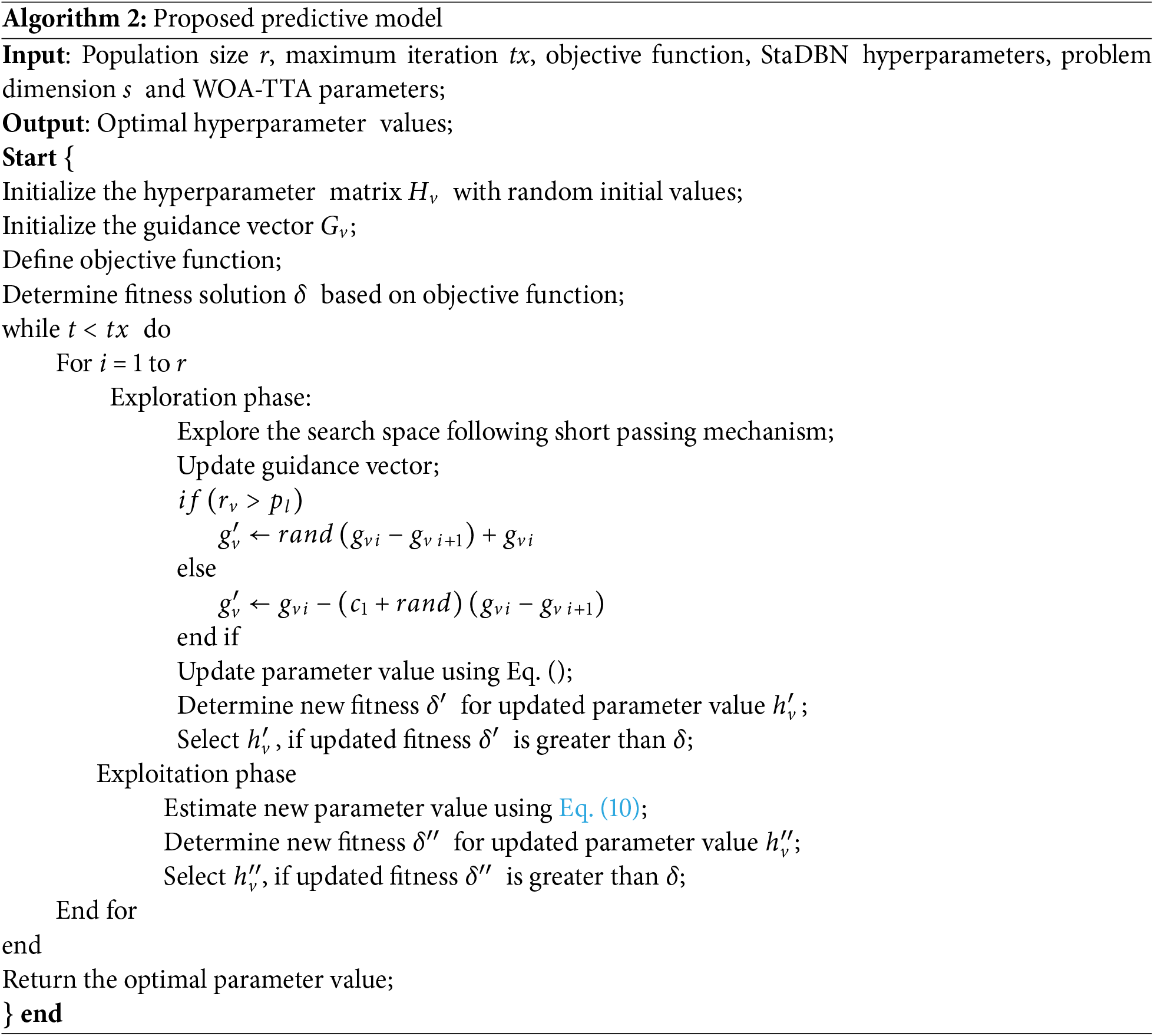
Hyperparameter optimization defines the process of finding the best value for StaDBN constraints such as batch size, learning rate, number of layers, training epochs, etc., to make training more efficient and less time consuming. In the study presented, a hybrid meta-heuristic optimizer named WOA-TTA was applied for refining StaDBN hyperparameters. This hybrid approach integrates the exploitation capacity of WOA and exploration efficiency of TTA into a single approach, resulting in better solutions for world optimization problems [33]. The whale optimization algorithm (WOA) is developed based on the hunting characteristics of humpback whales. These whales exhibit a unique exploitation strategy named “bubble-net behavior”, which mimics the circular and spiral-shaped motion of whales as they encircle prey. On the other hand, TTA is a meta-heuristic optimization algorithm inspired by football playing style. This method utilizes passing mechanisms that are short to provide a better exploration strategy. The integrated method is more efficient and stable compared to the traditional optimization models such as genetic algorithm, particle swarm optimization, Adam optimizer, etc., in the parameter optimization process, thus giving rise to superior prediction results. The hyperparameter optimization based on WOA-TTA consists of the following steps: (1) initialization of parameter population, (2) evaluation of fitness, (3) exploration phase, (4) exploitation phase, and (5) termination.

1. Initialization

This stage is the one that comes after the football team initialisation procedure in the TTA technique. In TTA the player’s position in the football team indicates the possible solution to the optimization problem created with s dimensions within the bound limit hence the ball position was also initialized as a vector that is responsible for guiding the player movement in the exploration stage. In the case of hyperparameter optimization, the football team represents the hyperparameter population, each player stands for the hyperparameter variable, the player’s position indicates the parameter value, and the ball position specifies the guidance vector, which directs the overall optimization process. The football team position and the ball position are initialized as matrix represented in Eqs. (21) and (22).

Hv=[hv1×1hv1×2⋯hv1×shv2×1hv2×2⋯hv2×s⋮⋮⋱⋮hvr×1hvr×2⋯hvr×s](21)

Gv=[gv1×1gv1×2⋯gv1×sgv2×1gv2×2⋯gv2×s⋮⋮⋱⋮gvr×1gvr×2⋯gvr×s](22)

where Hv denotes hyperparameter population, Gv represents the guidance vector, hv defines the position of the player in the population (parameter value), and r refers to the total number of players (population size).

2. Fitness/objective function evaluation

After initialization, the fitness function was determined for each player in the problem-solving space. The objective of the WOA-TTA is to reduce the prediction error (deviation between actual and predicted GQI) by continuously refining the parameter values in its training stage, which is formulated in Eq. (23).

Objectivefunction=min(Agqi−Ogqi)(23)

where Ogqi indicates the observed result and Agqi represents the actual outcome. Based on this function, the fitness solution was determined for the entire population Hv. The fitness solution obtained is expressed in Eq. (24).

δ=δ[hv1×1hv1×2⋯hv1×shv2×1hv2×2⋯hv2×s⋮⋮⋱⋮hvr×1hvr×2⋯hvr×s](24)

where δ indicates the fitness solution. Here, the parameter sequence of StaDBN with less error has high fitness and the solution with high error has lower fitness value. Subsequently, the best solution was determined by sorting the parameter solution based on their fitness value.

3. Exploration phase

The exploration stage follows the short passing mechanism of TTA technique. In this mechanism, the player will pass the ball to another nearby player to achieve the goal. Although the ball passing success rate is high, the chance of losing the ball to the opposite team also exists. In this process, both the position of the ball and the player gets updated forming new position. This update introduces changes in guidance vector as well as in the parameter value and it is mathematically defined in Eqs. (25) and (26).

gv′={rand(gvi−gvi+1)+gvi;rv>plgvi−(c1+rand)(gvi−gvi+1);rv≤pl(25)

hv′=hvi+rand∗c2∗(gvi′−hvi)+rand∗c3∗(h→−hvi)(26)

where rv represents the random number (0, 1), pl defines the probability of losing the ball to opposite team (0.1 to 0.3), gvi+1 denotes updated ith parameter’s guidance vector, gvi refers to the current ith parameter’s guidance vector, hvi indicates the current parameter value, hv′ defines updated parameter value, h→ refers to the best parameter value found based on initial fitness. Consequently, the fitness was determined for updated parameter solution and if the new fitness is greater than previous fitness, the updated parameter value is considered as best value, and it is used for StaDBN training.

4. Exploitation phase

In WOA-TTA, exploitation phase follows the bubble-net characteristics of humpback whales. In this phase, the parameter value is updated using two methods namely: shrinking encircling mechanism and spiral model. The parameter update process is formulated in Eq. (27).

hv′′={hvi−P→.D→;x<0.5D→.ebl.cos⁡(2πl)+hvi;x≥0.5(27)

where hv′′ denotes the updated parameter value in the exploitation phase, x indicates the random number (0, 1), P→ represents the coefficient vector, and D→ refers to the deviation between the best solution and the current solution. The formula for P→ is expressed in Eq. (28).

P→=2y→.z→−y→(28)

where y→ represents the control vector that decreases from 2 to 0, and z→ indicates the random vector [0, 1]. Further, the fitness solution was estimated for updated parameter solution and if the new fitness is greater than previous fitness, the updated parameter value is considered as optimal value.

5. Termination

This process of parameter update continues until reaching the maximum iteration count or maximum convergence rate. Thus, the WOA-TTA model returns the optimal values for each hyperparamater of StaDBN, which not only increases the prediction accuracy but also boosts the training speed. Algorithm 2 presents the working of the proposed predictive model in pseudocode format.

4.5 Evaluation Metrics

The performance of the devloped method is evaluated with the help of these metrics as stated in this subsection. The metrics, namely RMSE, NS, MAE, and R2, are defined and their formulas are given below.

1. Root Mean Square Error

RMSE evaluates the average magnitude of the error between predicted and observed values, and it is formulated in Eq. (29).

RMSE=1m∑i=1m(Ogqi−Agqi)2(29)

where Ogqi indicates the observed result and Agqi represents the actual outcome.

2. Mean Absolute Error

The average absolute difference between expected and actual values is measured by MAE. It is calculated using Eq. (30).

MAE=1m∑i=1m|Ogqi−Agqi|(30)

3. Nash-Sutcliffe efficiency

NS efficiency determines the predictive power of hydrological models. It compares the variance of prediction errors to the variance of the actual data, and it is defined in Eq. (31).

NS=1−∑i=1m(Ogqi−Agqi)2∑i=1m(Ogqi−Ogqi′)2(31)

where Ogqi′ indicates the Mean of observed values.

4. Correlation Coefficient

According to Eq. (32), the correlation coefficient quantifies the degree of linear correlation between observed and predicted values.

R=1−∑i=1m(Ogqi−Ogqi′)(Agqi−Agqi′)∑i=1m(Ogqi−Ogqi′)2∑i=1m(Agqi−Agqi′)2(32)

where Agqi′ represents the mean of actual values.

5. Root Mean Square–based Water Quality Index (RMS-WQI)

By combining several physicochemical and potentially poisonous element (PTE) factors into a single index value, the RMS-WQI was calculated to give an integrated quantitative assessment of overall groundwater quality. As shown below, the RMS-WQI formulation uses a multi-step process to guarantee reproducibility and transparency. To produce dimensionless quality ratios, each water quality parameter was first normalized in relation to its associated guideline or standard allowed limits (e.g., WHO drinking water standards). A quality score Qi was calculated for each parameter i as follows in Eq. (33).

Qi=CiSi(33)

where Ci is the parameter’s observed concentration and Si is its typical allowable limit. In order to highlight greater departures from allowable bounds, the normalized quality scores were then combined using a root mean square formulation is given in Eq. (34).

RMS−WQI=1n∑i=1nQi2(34)

where n is the total amount of water quality parameters considered. The RMS-based aggregation function tends to favor smaller deviations more significantly compared to the arithmetic averaging function and is therefore appropriate for simulating groundwater pollution due to industrial and air pollution. The computed RMS-WQIs can now be utilized for model training and prediction based on the target variable in order to facilitate direct comparison between the observed and predicted states of the groundwater. All the basic models and the new GWQP-StaDBN-WOA-TTA approach use an identical RMS-WQI calculation method for a fair comparison. The complex RMS-WQI calculation incorporated in the modeling approach has now been delineated within the methodology section for easy replication in any upcoming research pertaining to groundwater quality assessment.

The assessment of these metrics allows us to determine how precisely the presented approach predicts groundwater quality under multiple pollution sources.

5  Results and Discussion

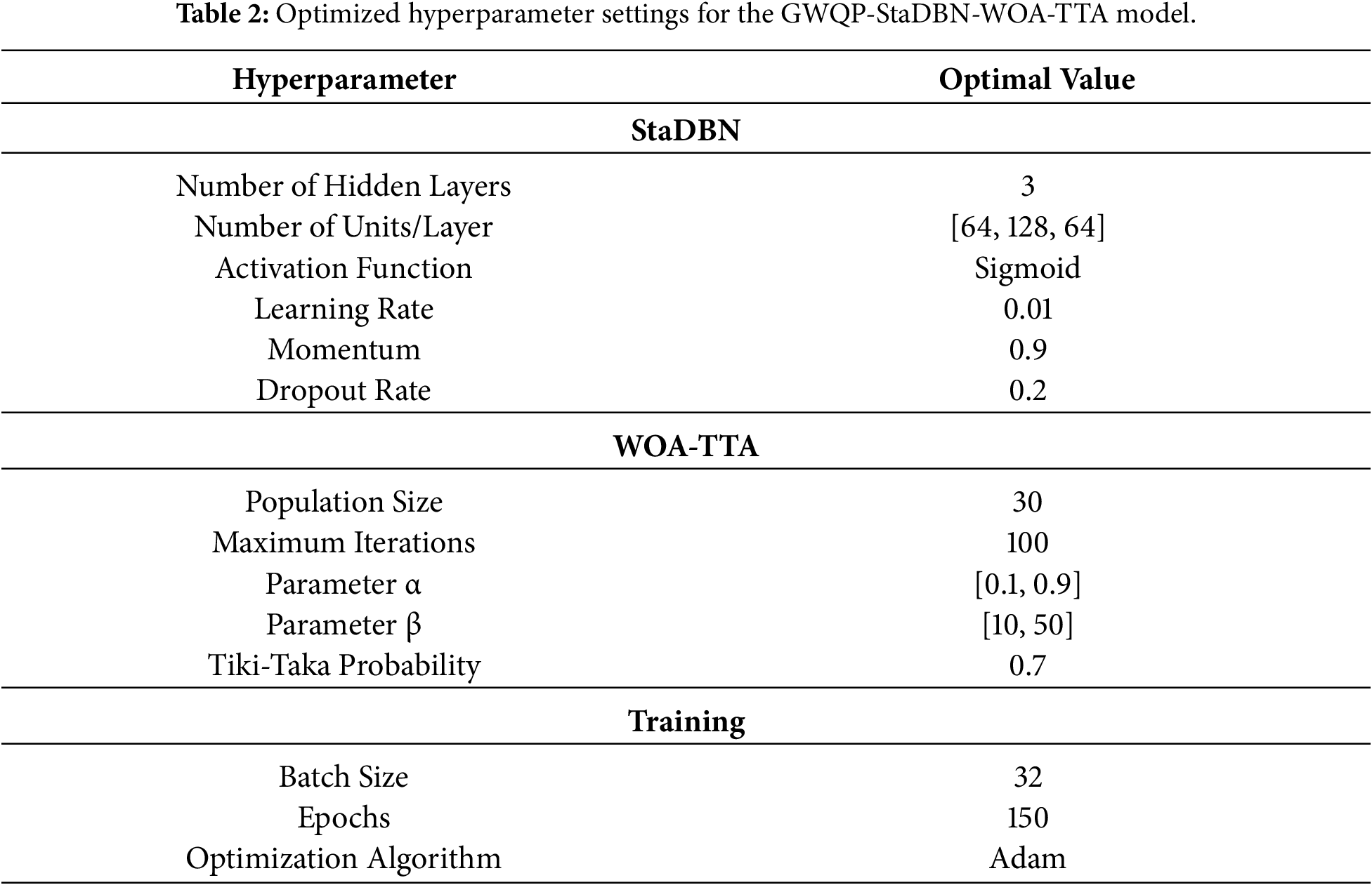
This study proposed an interpretable and explainable AI model for accurately predicting groundwater quality under multiple pollution sources. The novelty of the designed strategy lies in the seamless integration of WOA-TTA and StaDBN into a unified framework for predicting groundwater quality automatically with high accuracy and less computational time (GWQP-StaDBN-WOA-TTA). The presented methodology was implemented in Python and the results are obtained in terms of RMSE, NS, MAE and R. Finally, comparative validation against existing methods like Logistic Regression (LR), Support Vector Machine (SVM), Random Forest (RF), Adaptive Boosting (AdaBoost), and Extreme Gradient Boosting (XGBoost) (GWQP-LR-SVM-RF-AdaBoost-XGBoost) as documented in [23], artificial neural network (ANN), classification and regression tree (CART), random forest (RF), and support vector machine (SVM) (GWQP-ANN-CART-RF-SVM) [24] and GWQP-LSTM [27] underscored the superior performance achieved by the designed methodology. Table 2 illustrates the Optimized Hyperparameter Settings for the GWQP-StaDBN-WOA-TTA Model.

5.1 Experimental Setup

The PC used for the experiment has a 64-bit Windows 10 operating system, an Intel Core i7 processor, and 16 GB of RAM. The Python programming language was used for the application of the method. The data came from one single source—nine wells in Ishwardi Upazila, Pabna District, Bangladesh, which were monitored for groundwater quality levels. Besides, the dataset extended to covering the nine well spots for such water quality factors as Temperature, Electrical Conductivity, Total Dissolved Solids, pH, Total Hardness, and so on including heavy metals like Iron (Fe), Manganese (Mn), Chromium (Cr), Copper (Cu), Lead (Pb), Cadmium (Cd), and Arsenic (As). Data was divided into training and testing sets in 80:20 ratio. The performance of the proposed model GWQP-StaDBN-WOA-TTA was compared with the existing models such as GWQP-LR-SVM-RF-AdaBoost-XGBoost [23], GWQP-ANN-CART-RF-SVM [24] and GWQP-LSTM [27]. The comparison was made using the same evaluation metrics, namely RMSE, NS, MAE, and R, which were previously established.

5.2 Dataset Description

The dataset used in this study consists of groundwater quality records collected from nine monitoring wells located within the Rooppur Nuclear Power Plant (RNPP) operational area and its adjacent residential zones in Ishwardi Upazila, Pabna District, Bangladesh. Specifically, four wells (RN-W1 to RN-W4) are situated within the RNPP boundary, while five wells (RA-W1 to RA-W5) represent surrounding residential areas, enabling the assessment of both industrial and anthropogenic influences on groundwater quality.

Groundwater samples were obtained at an interval of sampling, such as monthly/seasonal (dry and wet seasons), suitable for the simulation of spatial and temporal models. Ground/surfacewater seasonal separation was used to reflect the hydraulic and pollutant transport cycle influenced by the recharge process of the rain and the concentration during the dry season.

Every groundwater sample contains physico-chemical variables like temperature, total dissolved solid (TDS), pH value, electrical conductivity (EC), total hardness (TH), and values of potentially toxic elements (PTEs), like iron (Fe), manganese (Mn), copper (Cu), lead (Pb), chromium (Cr), cadmium (Cd), and arsenic (As). This set of variables enables accurate modeling of the variations of groundwater quality influenced by different polluting factors.

The final dataset has been arranged in the form of multivariate time series data, in which every entry is related to a particular location and time point for data collection. This format allows for appropriate utilization of the proposed Spatial–Temporal-Assisted Deep Belief Network model for capturing spatial relations among various sites and understanding better the related patterns in time intervals.

Dataset Split Strategy and Randomness

The dataset of groundwater quality was split into training and testing groups with the ratio of 80:20 that is considered a common practice in environmental modeling and machine learning research in order to maintain a balance between the capacity of the model to learn and the objective evaluation of the model performance. The randomly selected split was done with a predetermined random seed to ensure that the study findings could be reproducible. By repairing the seed, it is possible to regenerate the same data partitions consistently, which can be fairly compared with future studies, and makes the evaluation of a model transparent.

To ensure no leakage of data, all the preprocessing was done only to the training data which consists of, filling in the missing values, outlier treatment, normalization and feature selection using the Addax Optimization Algorithm. The obtained preprocessing parameters were consequently applied to the testing data and were not re-estimated. This stringent segregation is used so that the testing set did not affect the model training or feature selection process.

In order to test the stability and ability of the model to generalize, one carried out a 10-fold cross-validation of its training data as well as the train test split. Ten mutually exclusive folds were randomly picked out of the dataset and they were applied on the validation and rest of the folds on training. This prevents variation in the performance estimates and also removes bias as a result of the one random split which is specifically crucial considering the small number of groundwater monitoring sites.

The splitting strategy adopted is suitable in the given study since it maintains statistical representative of the groundwater quality conditions in various seasons and places, reduces over-fitting, and offers a trustworthy estimation of predictive performance in the real-life pollution situations.

5.3 Performance Analysis of the Presented Approach

The baseline models used in the comparison i.e., ANN, RF, SVM, LSTM, and hybrid ensemble methods were selected due to the fact that they are commonly used in the research on groundwater quality prediction, and they represent both the traditional and deep learning paradigm. ANN, RF, and SVM are used to have standard comparisons with non-temporal modeling and LSTM accommodates the temporal dependence that is usually characteristic of hydrological data. Hybrid strategies were added so as to capture prior reported state of art performance on comparable datasets.

More complex architectures, such as attention-based networks, transformer networks, and GAN-enhanced networks, were not included in the direct comparison since such architectures are relatively less available in the public domain in terms of working implementations for groundwater prediction, in addition to some of these models being computationally intensive. Nevertheless, the drawbacks of these sophisticated models are also admitted, and the comparison with them is suggested as the extension in the future. The chosen strategy makes the comparison between it and methods used in the field to be fair, interpretable, and reproducible and to present the additional value of the proposed GWQP-StaDBN-WOA-TTA framework,

The box plots in this Fig. 2 below demonstrate the seasonal changes in Z-score scaled data for different GWQCs and potential trace elements (PTEs). From here onwards, every box plot in each figure may represent different variables such as: (a) Temperature, (b) pH, (c) Electrical Conductivity (EC), (d) Total Dissolved Solids (TDS), (e) Total Hardness (TH), (f) Iron (Fe), (g) Manganese (Mn), (h) Copper (Cu), (i) Lead (Pb), (j) Chromium (Cr), (k) Cadmium (Cd), and (l) Arsenic (As). Within each subplot, two box plots are presented by depicting the distribution of the Z-score scaled data during the dry and wet seasons. Median Z-scores and data spread generally differ between seasons by indicating temporal influences on concentrations with outliers present for some parameters. Total Dissolved Solids (TDS) shows consistent distributions across seasons, unlike other indicators exhibiting more pronounced seasonal shifts. Notably, PTE concentrations tend to be higher during the wet season possibly due to leaching from rainfall as suggested by upward shifts in the wet season box plots. Overall, Fig. 2 visually summarizes seasonal dynamics in Z-score scaled groundwater quality within the study area by complementing sble-3tistical table analyses.

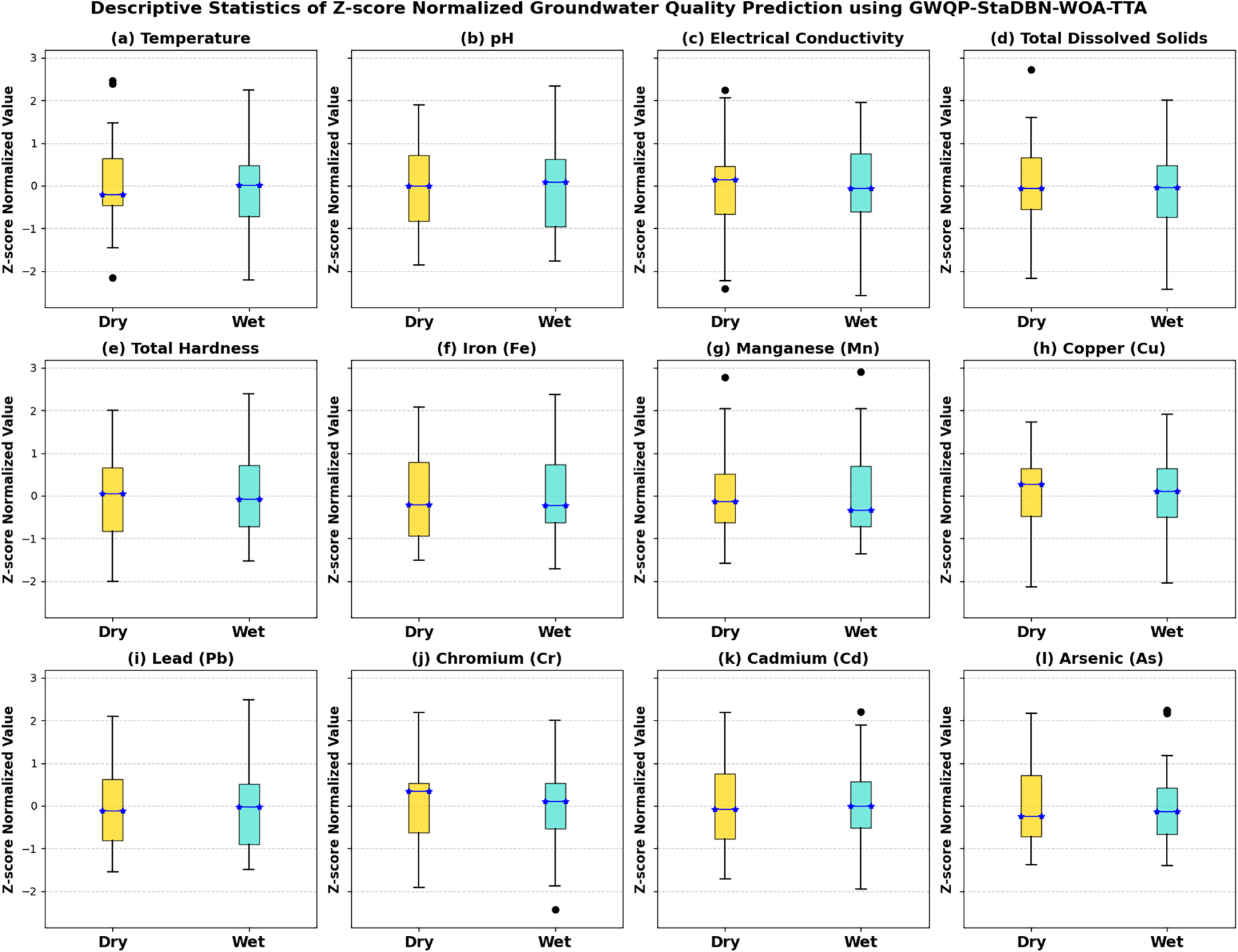
Figure 2: Z-score scaled concentrations of groundwater quality indicators and potential trace elements across dry and wet seasons.

The box plots in Fig. 3 present a statistical summary of the predicted RMS-WQI scores for the dry (a) and wet (b) seasons as determined by the proposed GWQP-StaDBN-WOA-TTA model. Each subplot displays the distribution of the predicted scores with the y-axis representing the RMS-WQI score ranging from 20 to 100. Horizontal dashed lines delineate water quality categories such as Limited (<30), Moderate (30–50), Satisfactory (50–80), and Excellent (80–100). For the dry season, the predicted RMS-WQI scores exhibit a central tendency around the ‘Satisfactory’ category, with some variability indicated by the interquartile range and whiskers. Similarly, the wet season predicted scores also fall primarily within the ‘Satisfactory’ range by showing a slightly higher median and a broader spread in comparison to the dry season predictions with an outlier present below the ‘Moderate’ threshold. Fig. 3 suggests that the model predicts a generally satisfactory groundwater quality based on PTE contamination assessment with a subtle indication of potentially lower quality or greater variability during the wet season in comparison to the dry season as inferred from the box plot characteristics relative to the defined water quality thresholds.

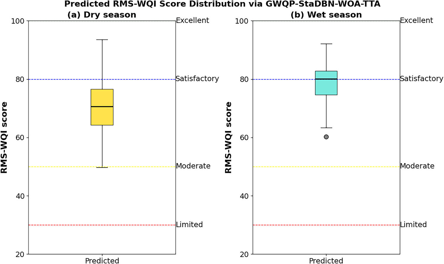
Figure 3: Statistical summary of predicted RMS-WQI scores across the study period for dry and wet seasons using GWQP-StaDBN-WOA-TTA.

Fig. 4 presents a location-specific comparison of predicted RMS-WQI scores at nine distinct groundwater locations (RN-W1 to RN-W4 within the RNPP operational area and RA-W1 to RA-W5 in the adjacent residential zone) for both dry and wet seasons as determined by the proposed GWQP-StaDBN-WOA-TTA model. The paired bars for each location allow for a direct assessment of seasonal variations in predicted water quality at individual points. Although most predicted scores reside within the ‘Satisfactory’ range across both seasons and locations, the plot highlights location-specific variations in the extent and direction of RMS-WQI changes between seasons. This visualization helps in identifying locations with more significant seasonal variability or consistently higher or lower predicted water quality relative to others within the study area. The spatial arrangement of these locations (within RNPP vs. residential area) allows for analysis concerning these predicted site-specific water quality patterns.

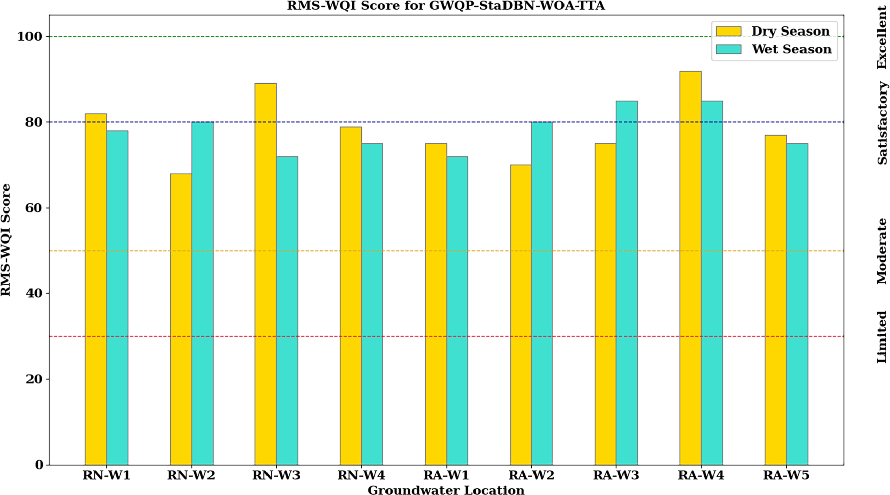
Figure 4: Predicted RMS-WQI scores across different groundwater locations during dry and wet seasons using GWQP-StaDBN-WOA-TTA.

Fig. 5 illustrates the 10-fold cross-validation effectiveness of the GWQP-StaDBN-WOA-TTA model across four key metrics such as RMSE, NSE, MAE, and Correlation Coefficient (R). Here, RMSE and MAE values indicators of prediction error are relatively low for both training and testing sets. The NSE and R values, which assess the model’s goodness of fit and correlation, are relatively high for both training and testing sets, indicating good predictive performance and reliable model generalization, without implying convergence toward the theoretical maximum value of 1. This suggests that the proposed GWQP-StaDBN-WOA-TTA model exhibits good predictive capability for groundwater quality parameters with consistent performance observed between the training and testing phases by indicating robust generalization ability and minimal overfitting.

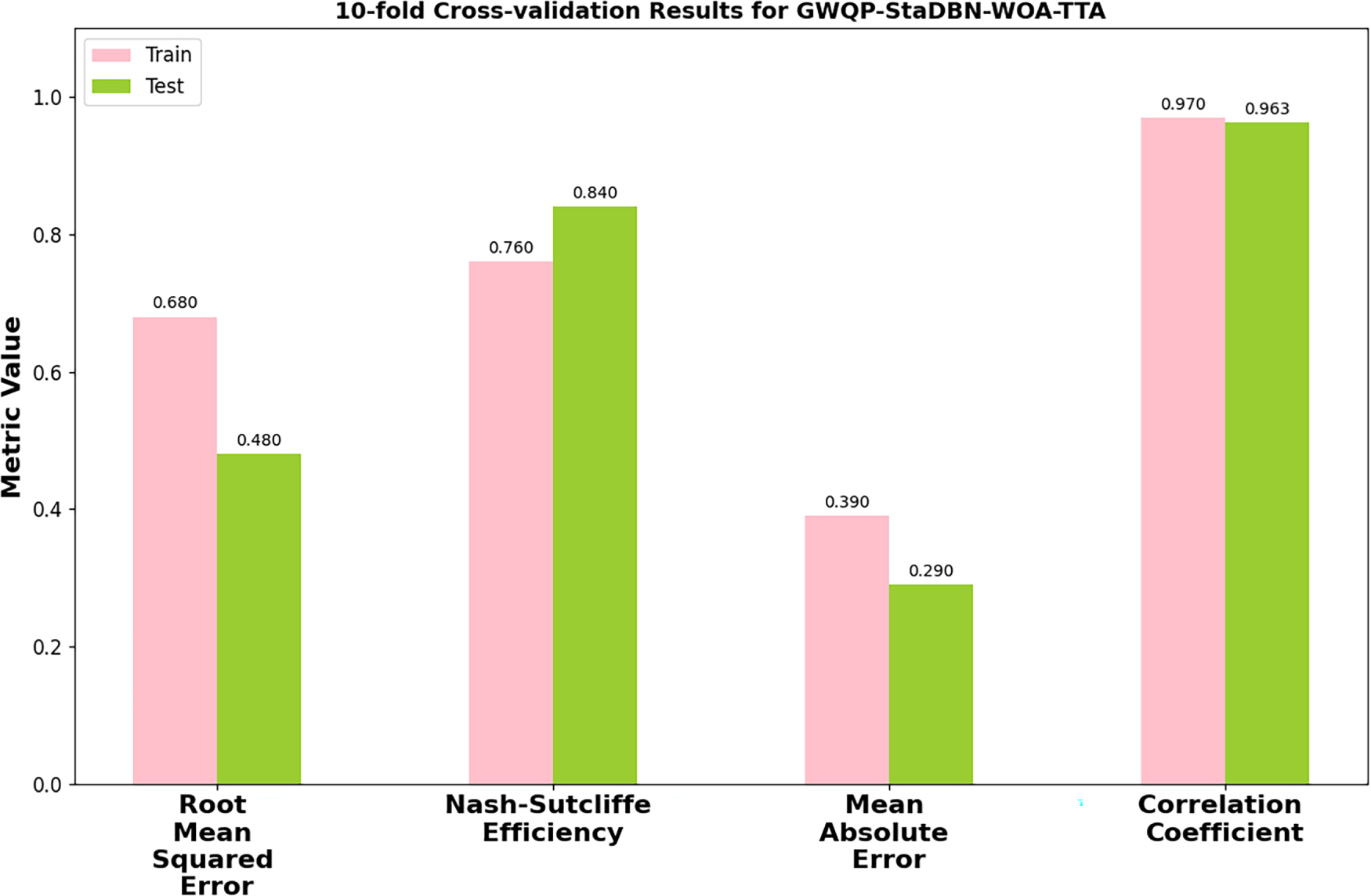
Figure 5: Ten-fold cross-validation performance of GWQP-StaDBN-WOA-TTA for predicting groundwater quality.

Fig. 6 presents Scatter plots comparing actual and predicted RMS-WQI values obtained through the proposed GWQP-StaDBN-WOA-TTA model during training and testing. Subplot (a) illustrates the model’s performance on the training dataset by indicating a strong positive correlation (R = 0.9702) between observed and modeled scores with data points closely distributed around the linear fit line. Subplot (b) displays the model’s predictive capability on the unseen testing dataset by revealing a similarly strong positive correlation (R = 0.9628) by suggesting effective generalization. The proximity of the linear fit lines to the perfect prediction line in both the training (a) and testing (b) subplots visually confirms the model’s accuracy in estimating RMS-WQI.

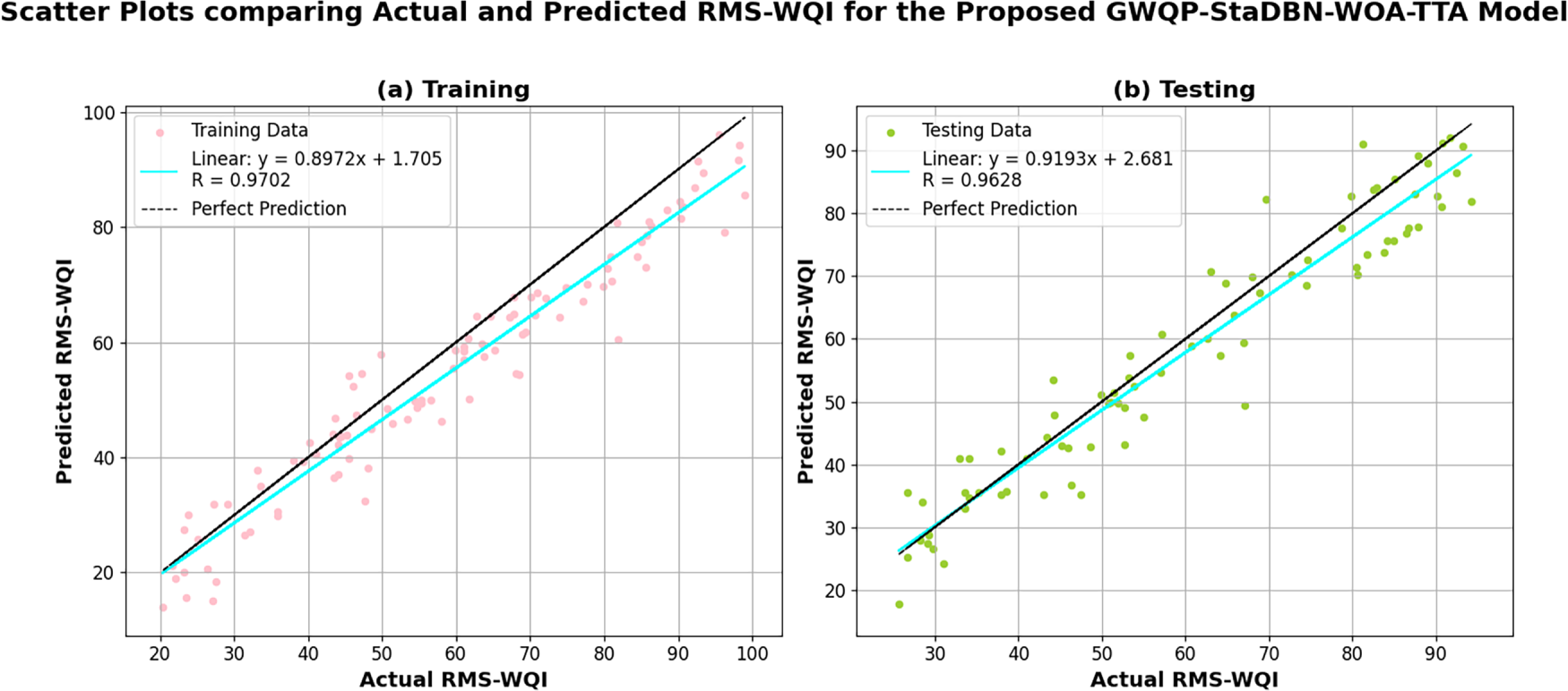
Figure 6: Scatter plots comparing actual and predicted RMS-WQI values obtained through the proposed GWQP-StaDBN-WOA-TTA model during training and testing.

Fig. 7 displays the relationship between Actual and predicted Water Quality Index (WQI) obtained through the proposed GWQP-StaDBN-WOA-TTA model during (a) the dry season and (b) the wet season. High R2 values such as 0.978 for the dry season and 0.990 for the wet season that indicate a strong correlation between actual and predicted WQI in both periods. The scatter plots show data points clustered closely around the solid line representing ideal prediction, where actual WQI equals predicted WQI. This close alignment suggests the model’s effectiveness in predicting WQI across different seasonal conditions.

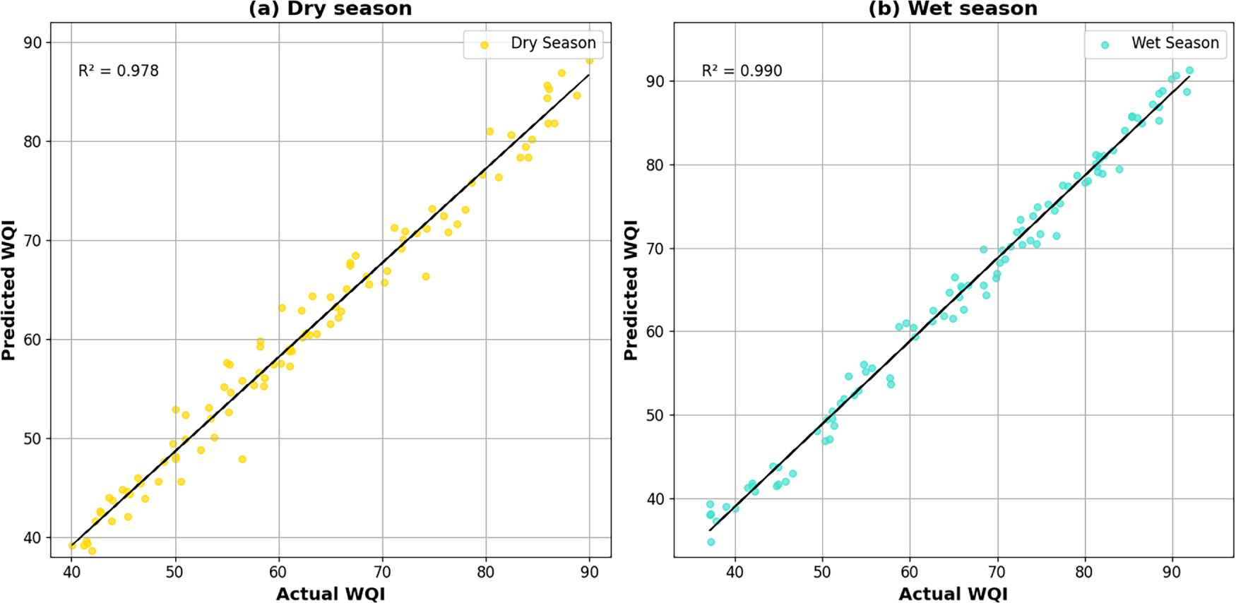
Figure 7: Scatter plots comparing the actual and predicted Water Quality Index (WQI) values for the proposed GWQP-StaDBN-WOA-TTA model during (a) the dry season and (b) the wet season.

The Spearman correlation matrix illustrated in Fig. 8 shows the statistical links that exist between z-scaled water quality parameters and the concentrations of potentially toxic elements (PTEs) in groundwater. This is all in accordance with the proposed GWQP-StaDBN-WOA-TTA framework. Here, distinct intra-element correlation appears between copper and cadmium. Excluding iron, lead, and arsenic, all examined PTEs show statistically significant associations with the analyzed water quality indicators. Notably, Manganese shows a strong positive correlation with electrical conductivity. Copper maintains a substantial positive association with temperature, total dissolved solids, and total hardness. Among the carcinogenic PTEs, chromium and cadmium reveal moderate positive correlations with total dissolved solids. These correlations indicate that the distribution patterns of PTEs in the groundwater are strongly governed by existing water quality conditions.

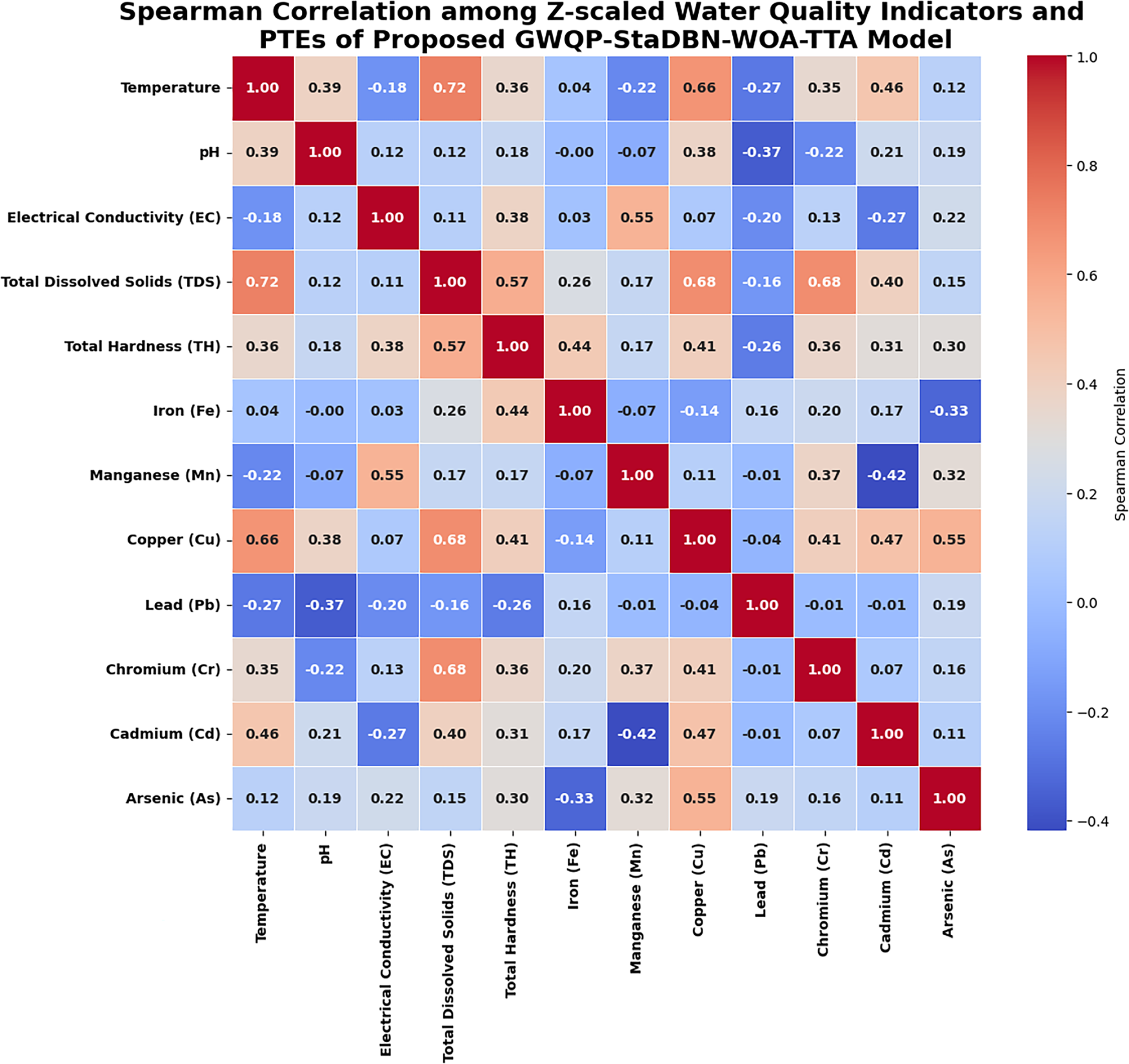
Figure 8: Spearman correlation matrix illustrates the relationships among z-scaled water quality indicators in the groundwater.

5.4 Comparative Validation

Figs. 9–12 present a comparative analysis of the proposed GWQP-StaDBN-WOA-TTA model against existing methodologies like GWQP-LR-SVM-RF-AdaBoost-XGBoost [23], GWQP-ANN-CART-RF-SVM [24] and GWQP-LSTM [27], respectively.

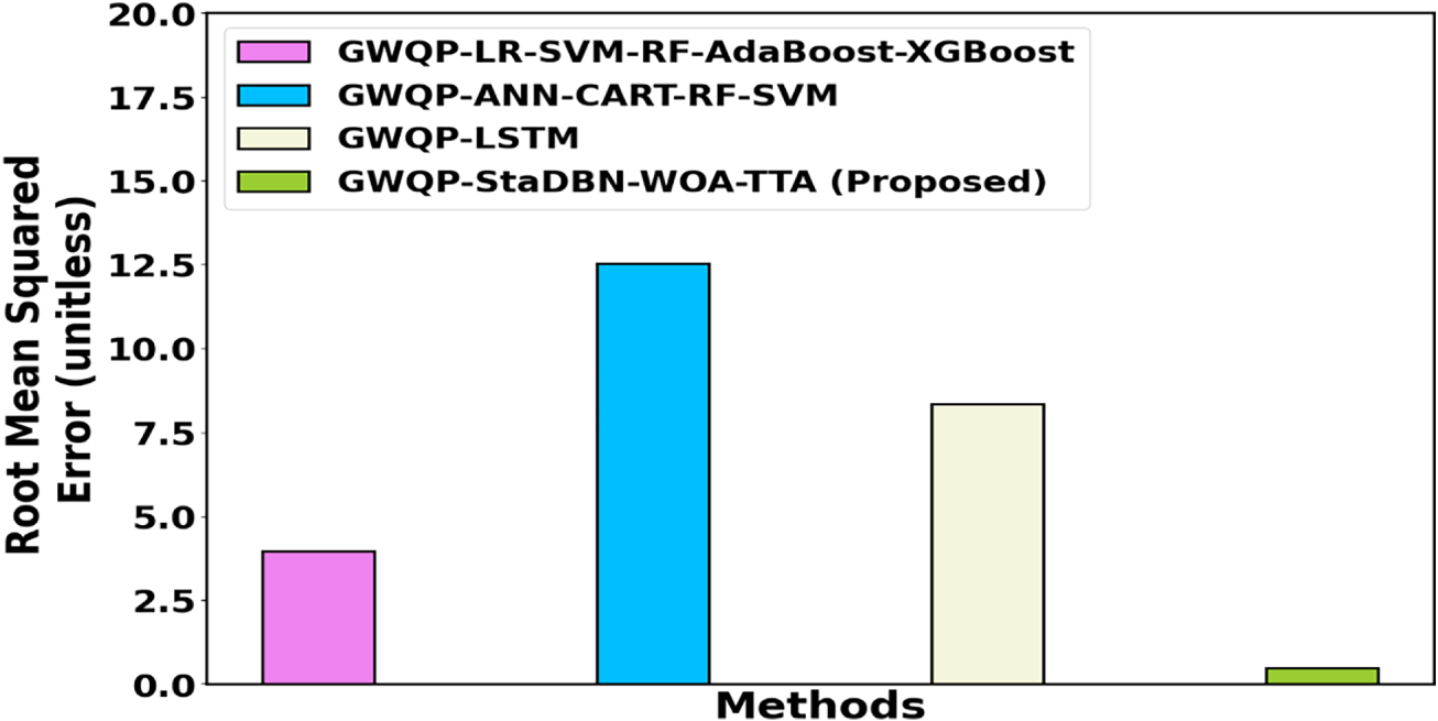
Figure 9: Comparison of Root Mean Squared Error (RMSE) for groundwater quality prediction models.

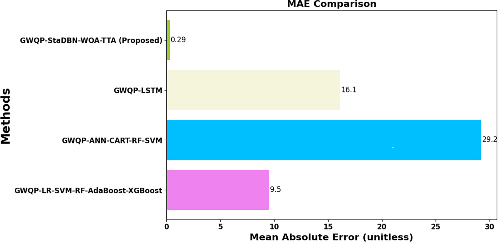
Figure 10: Comparison of Mean Absolute Error analysis for groundwater quality prediction models.

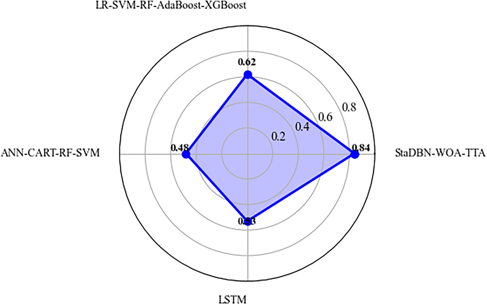
Figure 11: Comparison of Nash-Sutcliffe efficiency for groundwater quality prediction models.

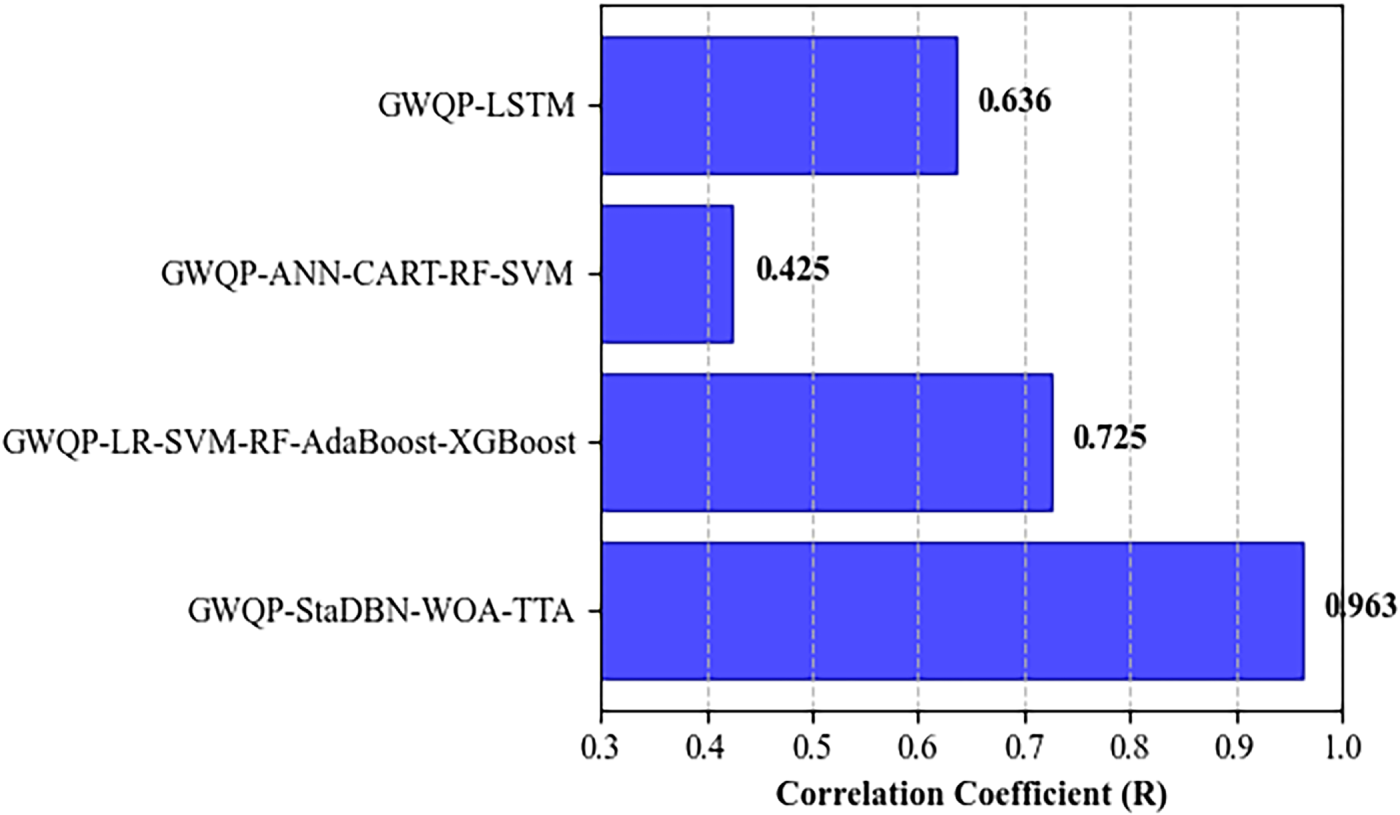
Figure 12: Comparison of correlation coefficient for groundwater quality prediction models.

Fig. 9 displays the root mean squared error (RMSE) for various groundwater quality prediction (GWQP) methodologies. Evaluated methods include GWQP-LR-SVM-RF-AdaBoost-XGBoost, GWQP-ANN-CART-RF-SVM, GWQP-LSTM, and the proposed GWQP-StaDBN-WOA-TTA. Notably, the proposed GWQP-StaDBN-WOA-TTA method achieves significantly lower RMSE values. Specifically, it attains 87.89%, 96.16%, and 94.25% lower RMSE in comparison with existing methodologies such as GWQP-LR-SVM-RF-AdaBoost-XGBoost, GWQP-ANN-CART-RF-SVM, and GWQP-LSTM, respectively.

Fig. 10 displays the Mean Absolute Error value for various groundwater quality prediction (GWQP) methodologies. Evaluated methods include GWQP-LR-SVM-RF-AdaBoost-XGBoost, GWQP-ANN-CART-RF-SVM, GWQP-LSTM, and the proposed GWQP-StaDBN-WOA-TTA. One of the significant results here is the much lower MAE values obtained through the proposed GWQP-StaDBN-WOA-TTA method. To be precise, the method highlights large MAE cuts by showing 96.94% less error when compared with GWQP-LR-SVM-RF-AdaBoost-XGBoost, 99.006% less error against GWQP-ANN-CART-RF-SVM, and 98.19% less error with respect to GWQP-LSTM. The work done proves the GWQP-StaDBN-WOA-TTA technique to be effective in the enhancement of prediction accuracy in groundwater quality area.

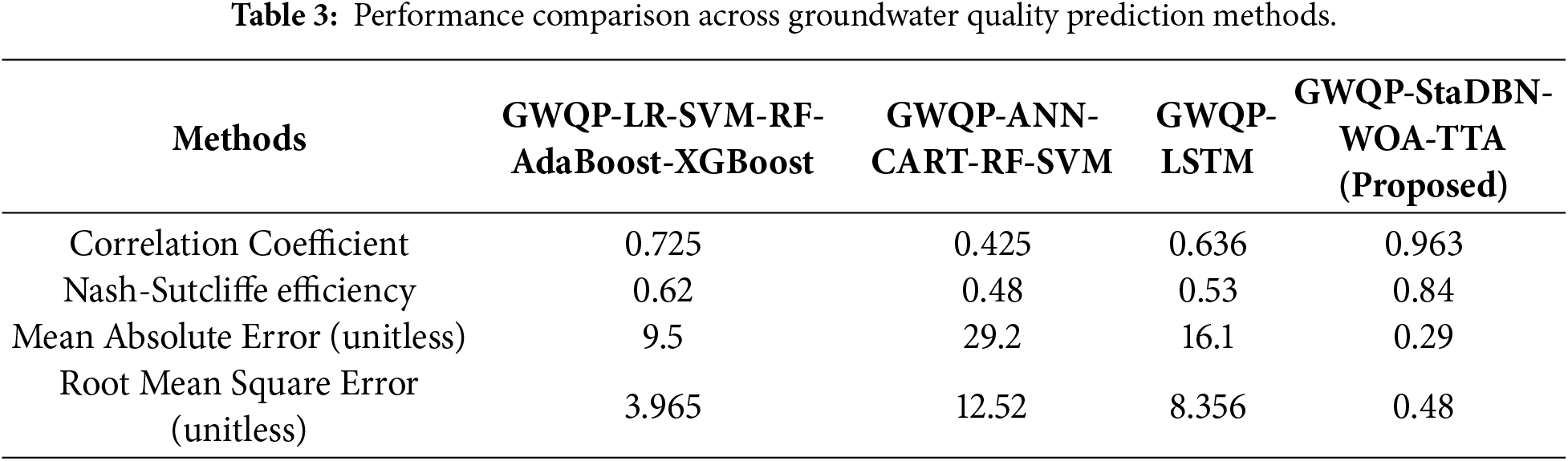
A comparative analysis of the Nash-Sutcliffe Efficiency (NSE) Fig. 11 presents a comparative analysis of Nash–Sutcliffe efficiency (NSE) across groundwater quality prediction models. The proposed GWQP-StaDBN-WOA-TTA framework achieves the highest NSE value (0.84), indicating superior predictive reliability and goodness of fit when compared with GWQP-LR-SVM-RF-AdaBoost-XGBoost (0.62), GWQP-ANN-CART-RF-SVM (0.48), and GWQP-LSTM (0.53). Such a result indicates the upswing in the prediction strength that comes along with the merging of StaDBN-WOA-TTA as a tool to assess groundwater quality.

Fig. 12 illustrates the comparative correlation coefficient (R) analysis for groundwater quality prediction models. The proposed GWQP-StaDBN-WOA-TTA model demonstrates the strongest linear agreement between predicted and observed values (R = 0.963), outperforming GWQP-LR-SVM-RF-AdaBoost-XGBoost (R = 0.725), GWQP-ANN-CART-RF-SVM (R = 0.425), and GWQP-LSTM (R = 0.636). These findings validate the increased predictive strengths in the strength of the suggested framework. The enhanced correlation through the high percentage gains reflects the enhanced reliability and accuracy of the GWQP-StaDBN-WOA-TTA method of detecting the underlying combinations of data.

The findings portray that, there is a moderate-to-strong positive relationship between the predicted and observed values of groundwater quality. In this study, the strength of correlation is interpreted using a quantitative classification scheme consistent with recent environmental modeling literature: very weak (|R| < 0.20), weak (0.20 ≤ |R| < 0.40), moderate (0.40 ≤ |R| < 0.60), strong (0.60 ≤ |R| < 0.80), and very strong (|R| ≥ 0.80). According to this taxonomy, the observed correlation coefficients values are within the moderate-to-strong positive range, and therefore it can be concluded that there is a significant linear relationship between the model predictions and the measured indicators of groundwater quality.

Quantitatively, such a degree of correlation suggests that the fluctuation in the quality of groundwater can be reasonably attributed to the parameter of physicochemical and potentially toxic elements chosen, but still permits inherent hydrogeological variability and uncertainty in measurement. Relative to the traditional models used as a baseline, where most of them have weak to moderate correlations, the proposed framework has a better explanatory capacity and predictive performance even in atmospheric and industrial pollution conditions.

5.5 Discussion

The research work proposes the A1 model GWQP-StaDBN-WOA-TTA and claims that it can provide interpetable and explainable approaches for the precise estimation of groundwater quality giving multiple pollution sources. The proposed GWQP-StaDBN-WOA-TTA approach is illustrated in a clear and repeatable manner to ensure easy replication in future work. Starting with data collection from groundwater observation wells, a series of data preparation tasks handling missing values, data normalization, and outlier processing are undertaken on the training dataset alone to avoid data leakage. Feature selection is conducted using the Addax Optimization Algorithm with clearly defined parameter settings and stopping criteria.

The Spatial–Temporal-Assisted Deep Belief Network (StaDBN) architecture is explicitly specified, including the amount of layers, neurons per layer, activation functions, learning rate, and training epochs. The WOA combined with Test-Time Augmentation (WOA–TTA) is employed for hyperparameter tuning, with initialization bounds, population size, and iteration limits clearly stated. Model training and validation follow a fixed random seed and an 80:20 train–test split strategy, supplemented by k-fold cross-validation to ensure robustness. The innovation of this methodology can be highlighted by acknowledging the synergy between WOA-TTA and StaDBN, the resulting automated groundwater quality prediction with high accuracy and shorter computing time. The proposed GWQP-StaDBN-WOA-TTA methodology is assessed by the followed figures and statistical tests which show its effectiveness. In Fig. 2, the temporal factors are shown and the wet season is commented concerning its likely leaching effects by depicting the seasonal changes in Z-score scaled groundwater quality indicators and PTE concentrations. A statistical summary of projected RMS-WQI scores is given in Fig. 3 by pointing out the generally good quality of groundwater with the possibility of lower quality or higher variability during the wet season. The specific location comparisons of predicted RMS-WQI scores shown in Fig. 4 show differences between various groundwater locations and seasonal changes in the study area. The performance of ten-fold cross-validation represented in Fig. 5 indicates the strong predictive power of the GWQP-StaDBN-WOA-TTA model with equal performance in training and testing phases by indicating strong generalization and small overfitting. Scatter plots shown in Fig. 6, which compare the real and predicted values of RMS-WQI, confirm the precision of the model in both the training and testing phases. The Fig. 7 seasonal scatter plots of the actual and predicted WQI scores also highlight the performance of the model through different seasons. The Spearman correlation matrix of Fig. 8 clarifies the interrelations between the water quality indicators and PTE concentrations in the groundwater, as it points towards a significant role of the existing water quality conditions in determining the PTE distribution patterns.

As shown in Figs. 9–12 and Table 3, the comparative validation against the existing methodologies accentuates the designed methodology’s superior performance. Fig. 9 reveals the RMSE values for the GWQP-StaDBN-WOA-TTA method to be 87.89%, 96.16% and 94.25% lower than those of GWQP-LR-SVM-RF-AdaBoost-XGBoost, GWQP-ANN-CART-RF-SVM, and GWQP-LSTM, respectively. Similarly, Fig. 10 discloses the MAE reductions achieved by the proposed method as 96.94%, 99.006%, and 98.19%, thus establishing its effectiveness in improving prediction accuracy. The major improvement in the GWQP-StaDBN-WOA-TTA model is shown in Fig. 11, where the NSE shows 35.48%, 75%, and 58.49%, meaning that the prediction capacity has improved. Finally, the proposed model in Fig. 12 reveals a much higher Correlation Coefficient value of 86.71%, 77.35%, and 84.84%, meaning that there is a higher linear correlation between the actual andpredicted values.

Performance assessment is carried out on established measures Correlation Coefficient (R), NSE, MAE, and RMSE with definitions provided in the methodological part. This level of procedure description also helps to ensure that a similar framework can be successfully developed again in an independent manner by other researchers in a similar scenario of groundwater quality evaluation.

Table 3 provides the comparative performance of the proposed GWQP-StaDBN-WOA-TTA and benchmark models and the results are now clearly presented in this section to enhance the transparency and clarity. In the process of revising the manuscript, it was revealed that certain of the values of the Correlation Coefficient reported in the previous version were out of range of −1 to 1 that is mathematically impossible. This problem was a tabulation reporting mismatch and not within the calculations. The correlation coefficients have also been re-checked and adjusted to meet the requirements of the statistical definitions and all the updated values are in the valid range.

In terms of the scale of the improvements that are reported, it is necessary to view the effectiveness gains of the proposed approach as the difference in methodologies, not as the dominance in percentages. The observed improvements arise from the combined effects of (i) spatial–temporal feature learning through the StaDBN architecture, (ii) optimized feature selection using the Addax Optimization Algorithm, and (iii) systematic hyperparameter tuning via WOA–TTA. Baseline models such as ANN, RF, and SVM rely on fixed or shallow representations and do not explicitly capture spatial and temporal dependencies, which explain their comparatively lower performance.

To avoid overstatement, the discussion has been revised to emphasize relative performance trends rather than excessive percentage gains. The corrected Table 3, together with Figs. 11–12, consistently shows that the proposed method achieves higher correlation and lower prediction errors while maintaining statistically valid and interpretable performance improvements over conventional models.

In this study, classification-style accuracy was not reported, as groundwater quality prediction is formulated as a regression problem rather than a classification task. Therefore, model performance was evaluated using regression accuracy metrics, namely the Correlation Coefficient (R), NSE, MAE, and RMSE, which are more appropriate for continuous-valued groundwater quality parameters.

For the testing dataset, the proposed GWQP-StaDBN-WOA-TTA model achieved a correlation coefficient of R = 0.963 and an NSE of 0.84, indicating strong agreement between observed and predicted values. The corresponding error metrics were MAE = 0.29 and RMSE = 0.48, reflecting low prediction error. These values represent the effective “prediction accuracy” of the model in a regression context and are consistently used for comparison with baseline models throughout the manuscript.

In conclusion, the seamless integration of WOA-TTA for hyperparameter optimization and StaDBN for spatial-temporal pattern learning within the GWQP-StaDBN-WOA-TTA framework yields significant improvements in groundwater quality prediction accuracy and reliability in comparison with conventional predictive models. The AI model that is interpretable and explainable can be considered a great instrument for the management of water resources in areas that are likely to be polluted by industries. Future research will investigate federated learning techniques. In particular, the privacy-preserving collaboration for modeling the groundwater contamination around the Rooppur Nuclear Power Plant (RNPP) using hydrochemical and possibly toxic element datasets from various monitoring sites and periods that have been vertically partitioned will be a very interesting area to explore. The advantage of this approach is that it allows the models to be trained together without sharing any data directly, thus solving the issues of privacy that come with sensitive environmental data.

6  Conclusion

This study developed an interpretable groundwater quality prediction framework, GWQP-StaDBN-WOA-TTA, to assess groundwater contamination influenced by atmospheric deposition and industrial activities in the RNPP region. The proposed model demonstrated superior predictive performance compared to conventional machine learning and deep learning baselines, achieving a correlation coefficient (R) of 0.963, Nash–Sutcliffe efficiency (NSE) of 0.84, and reduced prediction errors (MAE = 0.29, RMSE = 0.48) on the testing dataset. These results verify the capability of the proposed methodology in effectively identifying spatial-temporal correlations in the data and modeling the interactions of various substances in the groundwater system.

There are several limitations within this investigation, despite its robust performance. Firstly, more contemporary attention-based or transformer models were not considered for the comparative analysis, which only considered traditional and relatively complex deep learning architectures. Secondly, the data considered was limited to a particular geographical area and time frame, which may not be directly generalizable to other hydrogeological environments without retraining or calibration. Furthermore, this analysis was largely conducted for predictive aptitudes, as opposed to uncertainty or scenario-based probabilistic forecasting.

Additionally, despite the focus on the contamination of groundwater and the health implications put forth by the current research and the bulk of the literature that exists, the positive roles of the naturally occurring minerals (fluoride, chloride, zinc, and trace elements) have not been addressed. Notably, some of the recent studies emphasize the value of the risk-benefit approach and the fact that the levels of some of the minerals can positively affect human health. Incorporating both the beneficial and adverse effects of groundwater constituents represents an important future research direction.

Future studies should therefore focus on (i) benchmarking the proposed framework against advanced attention-driven and transformer-based models, (ii) integrating uncertainty and sensitivity analysis, (iii) extending the methodology to multi-regional and long-term datasets, and (iv) developing holistic groundwater quality assessment frameworks that simultaneously evaluate contamination risks and mineral-related health benefits, in line with emerging water sustainability research.

Acknowledgement: Not applicable.

Funding Statement: The authors extend their appreciation to University Higher Education Fund for funding this research work under Research Support Program for Central labs at King Khalid University through the project number CL/CO/B/6.

Author Contributions: Md. Mottahir Alam, Mohammed K. Al Mesfer, Haroonhaider Sidhwa, Mohd Danish: conceptualization, visualization, investigation, methodology, writing—original draft. Asif Irshad Khan, Tauheed Khan Mohd: resources, supervision, data curation, software, validation, writing—review & editing. Mohammed K. Al Mesfer: Funding. All authors reviewed and approved the final version of the manuscript.

Availability of Data and Materials: The datasets used and/or analyzed during the current study are available from the corresponding author upon reasonable request.

Ethics Approval: Not applicable.

Conflicts of Interest: The authors declare no conflicts of interest.

Code Availability: The computational workflow and algorithmic details are fully described in the manuscript. Source code may be provided upon reasonable request, subject to institutional policies.

Nomenclature

References

1. Lapworth DJ, Boving TB, Kreamer DK, Kebede S, Smedley PL. Groundwater quality: global threats, opportunities and realising the potential of groundwater. Sci Total Environ. 2022;811(2):152471. doi:10.1016/j.scitotenv.2021.152471. [Google Scholar] [PubMed] [CrossRef]

2. Sarker B, Keya KN, Mahir FI, Nahiun KM, Shahida S, Khan RA. Surface and ground water pollution: causes and effects of urbanization and industrialization in south Asia. Sci Rev. 2021;2021(73):32–41. doi:10.32861/sr.73.32.41. [Google Scholar] [CrossRef]

3. Kayastha V, Patel J, Kathrani N, Varjani S, Bilal M, Show PL, et al. New Insights in factors affecting ground water quality with focus on health risk assessment and remediation techniques. Environ Res. 2022;212(Pt A):113171. doi:10.1016/j.envres.2022.113171. [Google Scholar] [PubMed] [CrossRef]

4. Karunanidhi D, Subramani T, Roy PD, Li H. Impact of groundwater contamination on human health. Environ Geochem Health. 2021;43(2):643–7. doi:10.1007/s10653-021-00824-2. [Google Scholar] [PubMed] [CrossRef]

5. Naz I, Ahmad I, Aslam RW, Quddoos A, Yaseen A. Integrated assessment and geostatistical evaluation of groundwater quality through water quality indices. Water. 2024;16(1):63. doi:10.3390/w16010063. [Google Scholar] [CrossRef]

6. Najafzadeh M, Homaei F, Mohamadi S. Reliability evaluation of groundwater quality index using data-driven models. Environ Sci Pollut Res Int. 2022;29(6):8174–90. doi:10.1007/s11356-021-16158-6. [Google Scholar] [PubMed] [CrossRef]

7. Arifullah, Huang C, Akram W, Rashid A, Ullah Z, Shah M, et al. Quality assessment of groundwater based on geochemical modelling and water quality index (WQI). Water. 2022;14(23):3888. doi:10.3390/w14233888. [Google Scholar] [CrossRef]

8. Rajeev A, Shah R, Shah P, Shah M, Nanavaty R. The potential of big data and machine learning for ground water quality assessment and prediction. Arch Comput Meth Eng. 2025;32(2):927–41. doi:10.1007/s11831-024-10156-w. [Google Scholar] [CrossRef]

9. Zhu M, Wang J, Yang X, Zhang Y, Zhang L, Ren H, et al. A review of the application of machine learning in water quality evaluation. Eco Environ Health. 2022;1(2):107–16. doi:10.1016/j.eehl.2022.06.001. [Google Scholar] [PubMed] [CrossRef]

10. Karim MR, Shajalal M, Graß A, Döhmen T, Chala SA, Boden A, et al. Interpreting black-box machine learning models for high dimensional datasets. In: Proceedings of the 2023 IEEE 10th International Conference on Data Science and Advanced Analytics (DSAA); 2023 Oct 9–13; Thessaloniki, Greece. doi:10.1109/DSAA60987.2023.10302562. [Google Scholar] [CrossRef]

11. ŞAHiN E, Arslan NN, Özdemir D. Unlocking the black box: an in-depth review on interpretability, explainability, and reliability in deep learning. Neural Comput Appl. 2025;37(2):859–965. doi:10.1007/s00521-024-10437-2. [Google Scholar] [CrossRef]

12. Hassija V, Chamola V, Mahapatra A, Singal A, Goel D, Huang K, et al. Interpreting black-box models: a review on explainable artificial intelligence. Cogn Comput. 2024;16(1):45–74. doi:10.1007/s12559-023-10179-8. [Google Scholar] [CrossRef]

13. Sarker IH. Machine learning: algorithms, real-world applications and research directions. SN Comput Sci. 2021;2(3):160. doi:10.1007/s42979-021-00592-x. [Google Scholar] [PubMed] [CrossRef]

14. Madani A, Hagage M, Elbeih SF. Random Forest and Logistic Regression algorithms for prediction of groundwater contamination using ammonia concentration. Arab J Geosci. 2022;15(20):1619. doi:10.1007/s12517-022-10872-2. [Google Scholar] [CrossRef]

15. Subba Rao N, Das R, Gugulothu S. Understanding the factors contributing to groundwater salinity in the coastal region of Andhra Pradesh, India. J Contam Hydrol. 2022;250:104053. doi:10.1016/j.jconhyd.2022.104053. [Google Scholar] [PubMed] [CrossRef]

16. Torres-Martínez JA, Mahlknecht J, Kumar M, Loge FJ, Kaown D. Advancing groundwater quality predictions: machine learning challenges and solutions. Sci Total Environ. 2024;949:174973. doi:10.1016/j.scitotenv.2024.174973. [Google Scholar] [PubMed] [CrossRef]

17. Tao H, Hameed MM, Marhoon HA, Zounemat-Kermani M, Heddam S, Kim S, et al. Groundwater level prediction using machine learning models: a comprehensive review. Neurocomputing. 2022;489(1):271–308. doi:10.1016/j.neucom.2022.03.014. [Google Scholar] [CrossRef]

18. Moayedi H, Salari M, Dehrashid AA, Le BN. Groundwater quality evaluation using hybrid model of the multi-layer perceptron combined with neural-evolutionary regression techniques: case study of Shiraz plain. Stoch Environ Res Risk Assess. 2023;37(8):2961–76. doi:10.1007/s00477-023-02429-w. [Google Scholar] [CrossRef]

19. Hanoon MS, Ahmed AN, Fai CM, Birima AH, Razzaq A, Sherif M, et al. Application of artificial intelligence models for modeling water quality in groundwater: comprehensive review, evaluation and future trends. Water Air Soil Pollut. 2021;232(10):411. doi:10.1007/s11270-021-05311-z. [Google Scholar] [CrossRef]

20. Pandya H, Jaiswal K, Shah M. A comprehensive review of machine learning algorithms and its application in groundwater quality prediction. Arch Comput Meth Eng. 2024;31(8):4633–54. doi:10.1007/s11831-024-10126-2. [Google Scholar] [CrossRef]

21. Alizamir M, Kazemi Z, Kazemi Z, Kermani M, Kim S, Heddam S, et al. Investigating landfill leachate and groundwater quality prediction using a robust integrated artificial intelligence model: grey wolf metaheuristic optimization algorithm and extreme learning machine. Water. 2023;15(13):2453. doi:10.3390/w15132453. [Google Scholar] [CrossRef]

22. Singha S, Pasupuleti S, Singha SS, Singh R, Kumar S. Prediction of groundwater quality using efficient machine learning technique. Chemosphere. 2021;276:130265. doi:10.1016/j.chemosphere.2021.130265. [Google Scholar] [PubMed] [CrossRef]

23. Karunanidhi D, Raj MRH, Roy PD, Subramani T. Integrated machine learning based groundwater quality prediction through groundwater quality index for drinking purposes in a semi-arid river basin of south India. Environ Geochem Health. 2025;47(4):119. doi:10.1007/s10653-025-02425-9. [Google Scholar] [PubMed] [CrossRef]

24. Lee JM, Ko KS, Yoo K. A machine learning-based approach to predict groundwater nitrate susceptibility using field measurements and hydrogeological variables in the Nonsan Stream Watershed, South Korea. Appl Water Sci. 2023;13(12):242. doi:10.1007/s13201-023-02043-9. [Google Scholar] [CrossRef]

25. Xiong Y, Luo J, Liu X, Liu Y, Xin X, Wang S. Machine learning-based optimal design of groundwater pollution monitoring network. Environ Res. 2022;211:113022. doi:10.1016/j.envres.2022.113022. [Google Scholar] [PubMed] [CrossRef]

26. Valadkhan D, Moghaddasi R, Mohammadinejad A. Groundwater quality prediction based on LSTM RNN: an Iranian experience. Int J Environ Sci Technol. 2022;19(11):11397–408. doi:10.1007/s13762-022-04356-9. [Google Scholar] [PubMed] [CrossRef]

27. Kasiselvanathan M, Venkata Siva Rama Prasad C, Vijay Arputharaj J, Suresh A, Sinduja M, Prajna KB, et al. Prediction of ground water quality in western regions of Tamilnadu using LSTM network. Groundw Sustain Dev. 2024;25(1):101156. doi:10.1016/j.gsd.2024.101156. [Google Scholar] [CrossRef]

28. Kulisz M, Kujawska J, Przysucha B, Cel W. Forecasting water quality index in groundwater using artificial neural network. Energies. 2021;14(18):5875. doi:10.3390/en14185875. [Google Scholar] [CrossRef]

29. Uddin MG, Imran MH, Sajib AM, Abu Hasan M, Diganta MTM, Dabrowski T, et al. Assessment of human health risk from potentially toxic elements and predicting groundwater contamination using machine learning approaches. J Contam Hydrol. 2024;261(2):104307. doi:10.1016/j.jconhyd.2024.104307. [Google Scholar] [PubMed] [CrossRef]

30. Rodríguez-Murillo JC, Filella M. Significance and causality in continuous wavelet and wavelet coherence spectra applied to hydrological time series. Hydrology. 2020;7(4):82. doi:10.3390/hydrology7040082. [Google Scholar] [CrossRef]

31. Hamadneh T, Kaabneh K, Alssayed O, Eguchi K, Gochhait S, Leonova I, et al. Addax optimization algorithm: a novel nature-inspired optimizer for solving engineering applications. Int J Intell Eng Syst. 2024;17(3):732–43. doi:10.22266/ijies2024.0630.57. [Google Scholar] [CrossRef]

32. Zhao H, Liu J, Chen H, Chen J, Li Y, Xu J, et al. Intelligent diagnosis using continuous wavelet transform and Gauss convolutional deep belief network. IEEE Trans Reliab. 2023;72(2):692–702. doi:10.1109/TR.2022.3180273. [Google Scholar] [CrossRef]

33. Najm HY, Khaleel ES, Hamed ET, Ahmed HI. HWOA-TTA: a new hybrid metaheuristic algorithm for global optimization and engineering design applications. Int J Math Math Sci. 2024;2024(1):9140405. doi:10.1155/2024/9140405. [Google Scholar] [CrossRef]