
 Login
Login Register
 Submit a Paper
 Propose a Special lssue
 Open Access
ARTICLE

A Lagrangian Generalized Finite Difference Method for the Bubble Flow with Large Density Difference Considering the Continuous Surface Force Model
School of Naval Architecture, Ocean and Energy Power Engineering, Wuhan University of Technology, Wuhan, China
* Corresponding Author: Yongou Zhang. Email:
(This article belongs to the Special Issue: Recent Developments in Nonlocal Meshfree Particle Methods for Solids and Fluids )
Computer Modeling in Engineering & Sciences 2026, 148(1), 10 https://doi.org/10.32604/cmes.2026.082363
Received 14 March 2026; Accepted 11 June 2026; Issue published 27 July 2026
 View Full Text
 Download PDF
Abstract
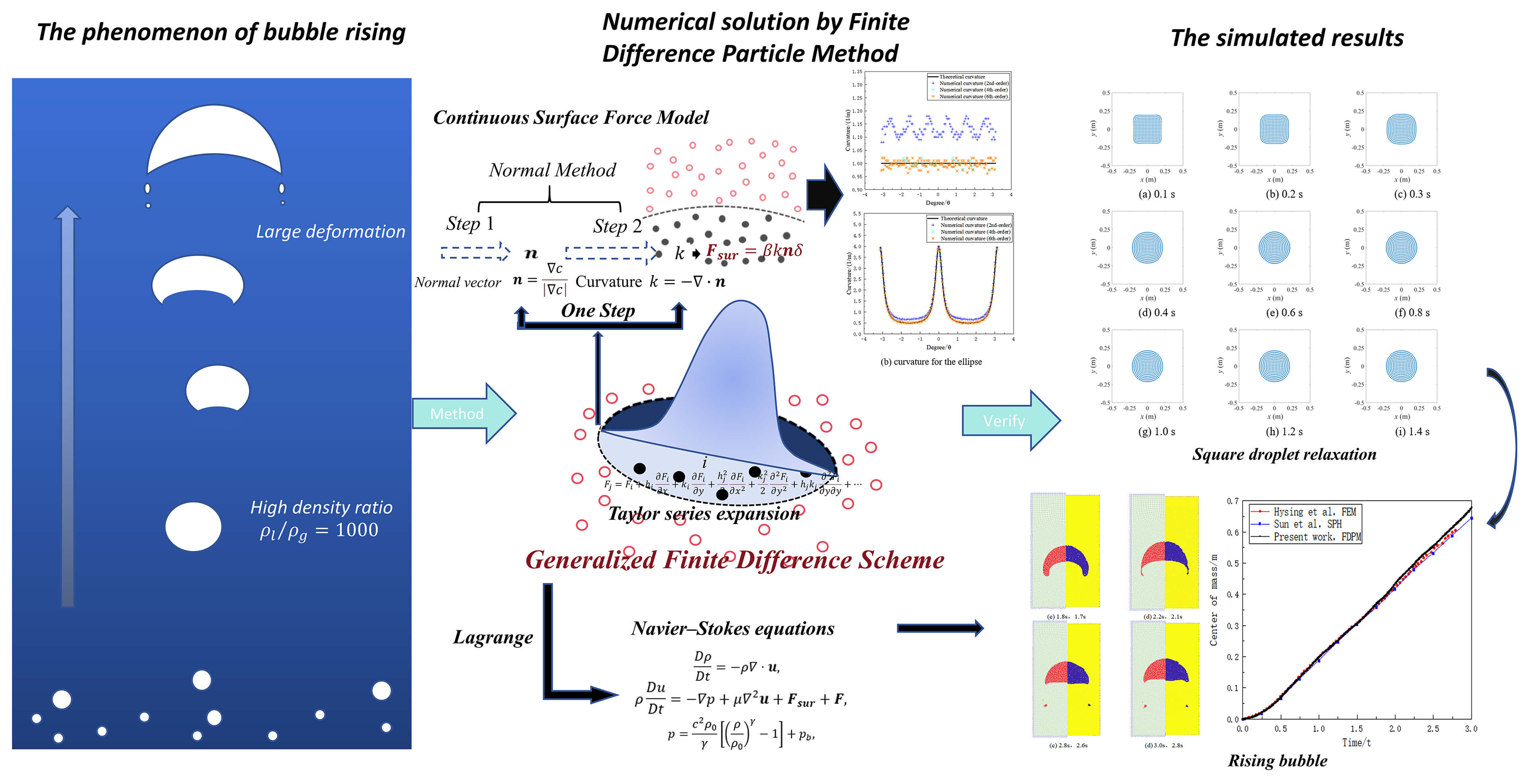
Due to the complex and dynamic nature of multi-phase interfaces, accurately capturing interface evolution remains one of the key challenges in multi-phase flow simulations, particularly in modeling bubble rising. In this study, a fully Lagrangian method is developed by using the Generalized Finite Difference (GFD) scheme, which we refer to as Finite Difference Particle Method (FDPM), and the Continuum Surface Force (CSF) model to simulate bubble dynamics. In this framework, the fluid is represented by particles, and all partial differential terms in the Navier–Stokes equations are discretized into symmetric linear systems using the GFD scheme. Notably, the interface curvature required by the CSF model is computed directly via the Laplacian of the color function, rather than through the divergence of the unit normal vector. The bubble relaxation cases with various density ratios (up to 1000) are tested, revealing that the pressure distributions inside and outside the bubbles generally agree with theoretical predictions. Finally, simulations of rising bubbles with a high density ratio (1:1000) and Reynolds number of 25 demonstrate that the time evolution of the bubble’s center of mass by FDPM is consistent with results obtained by the Smoothed Particle Hydrodynamics (SPH) and the Finite Element Method (FEM) approaches.Graphic Abstract
Keywords
Bubble dynamics in two-phase flows are governed by a variety of interacting factors, including gravity, surface tension, pressure, and viscous forces, resulting in a nonlinear process characterized by complex internal flows and dynamic interface deformations. Under these influences, bubbles may undergo phenomena such as breakup, coalescence, and other intricate interface evolutions. This phenomenon is not only ubiquitous in nature, but also actively utilized or deliberately suppressed in engineering fields such as marine engineering, chemical processing, and the food industry [1–3]. Therefore, the complexity and broad relevance of bubble dynamics make it a scientifically important and challenging subject of research.
The numerical study of bubble dynamics primarily relies on accurately simulating bubble motion and capturing interface evolution. In the field of computational fluid dynamics (CFD), Eulerian methods are widely adopted owing to their conservative properties and the ease of achieving high-order accuracy. However, these methods often face difficulties in accurately capturing or tracking bubble interfaces in the early time. To address this issue, various interface-capturing techniques have been developed, such as the Volume of Fluid (VOF) method [4,5], VOF coupled with the Level-Set method [6,7], and VOF coupled with Front-Tracking methods [8,9], all of which have demonstrated promising results. On the other hand, Lagrangian meshfree methods, owing to their special physical foundations, are getting more attention on bubble problems in recent years, such as the Smoothed Particle Hydrodynamics (SPH) [10], the Moving Particle Semi-implicit (MPS) [11] and Dissipative Particle Dynamics (DPD) methods [12]. These methods are inherently suitable for handling large deformations, as well as interface merging and tearing [13–17], making them particularly advantageous in the numerical study of bubble dynamics [18–21].
Lagrangian meshfree methods simulate fluid flow by employing a set of discrete particles that carry physical properties. The simulation of natural flow fields is achieved by updating both the particle positions and their associated physical quantities. In the numerical study of bubble two-phase flows using Lagrangian meshfree approaches, the modeling of surface tension and the treatment of viscous terms at the fluid interface are two critical challenges [22].
Currently, two mainstream approaches are employed to handle surface tension. The first category is based on inter-particle force models [23], which are simple and effective but heavily reliant on empirical coefficients, limiting their applicability in large-scale or generalized simulations. The second category adopts the Continuum Surface Force (CSF) model [24], wherein surface tension is modeled as being proportional to the local interface curvature. The accuracy of this method thus depends on the precise evaluation of curvature. Within meshfree frameworks, the CSF model commonly utilizes a color function to facilitate the divergence calculation of the unit normal vector to the interface [25]. This enables more reliable curvature computation from the interface normals. In early SPH formulations, direct curvature calculation often amplified numerical errors, necessitating smoothing of the unit normal vectors to enhance computational stability and accuracy [15]. Additionally, it has been observed that high density ratios adversely affect curvature accuracy. As a result, density-corrected color functions have been introduced to better capture asymmetric distributions of surface tension [22].
To address the viscous approximation near two-phase interfaces, Grenier et al. [25] introduced a shelter correction function into the SPH method, aimed at improving simulations involving both interfaces and free-surface flows. Grenier et al. [26] later extended this multiphase formulation by examining both harmonic and arithmetic means for viscous term approximations, demonstrating that the harmonic mean yields higher accuracy. Building upon these advancements, numerous modified models have been developed for bubble dynamics within Lagrangian meshfree frameworks, further expanding their applicability [16,17,27,28].
Based on the above review, the resolution of surface tension at the bubble interface relies heavily on the calculation of the gradient of the color function, whose accuracy and robustness are closely related to the computation of partial differential operators. In early SPH methods, Morris [14] found that directly calculating curvature from sharp color functions would amplify numerical errors. Using normal vector smoothing can improve the accuracy of curvature calculation. So many multiphase flow numerical methods rely on first-order differential operators, which are computationally more expensive to capture interface information. However, studies have shown that the Generalized Finite Difference (GFD) scheme can solve partial differential equations with high accuracy and computational efficiency [29–32]. GFD is a mesh-free local collocation method, which constructs the discrete form of PDEs based on Taylor series expansion of the field variables, and uses the Moving Least Squares (MLS) technique to minimize truncation errors. For instance, Prieto et al. [33] applied the GFD method to solve the advection-diffusion equation using an explicit scheme, and investigated the convergence and truncation error on irregular grids. Later, Li and Fan [34] proposed a new meshfree numerical method based on the GFD framework to accurately solve two-dimensional shallow water equations. In the Lagrangian framework, Seibold [35] investigated the properties of the M-matrix in finite difference schemes and conducted a comparative study on different least-squares formulations. Tiwari and Kuhnert [36] proposed a meshfree particle method, based on the Finite Pointset Method (FPM), which incorporates surface tension effects and was validated through the Laplace law and Rayleigh–Taylor instability tests. Huang et al. [37] proposed a new FPM scheme. This method is a kernel gradient-free (KGF) SPH method. It is based on Taylor series expansion and solves hydrodynamic problems without computing kernel gradients. Lu et al. [38] demonstrated that the FPM based on the least-squares approach can simulate complex free-surface flows efficiently and accurately. Zhang and Xiong [39] developed a pure Lagrangian meshfree particle method based on the GFD scheme named Finite Difference Particle Method for simulating weakly compressible viscous single-phase flows, in which fluid motion is described by Lagrangian particles and the differential operators in the Navier–Stokes equations are discretized into a symmetric linear system using the GFD formulation. In addition, Joubert et al. [40] developed a multiphase flow solver based on the GFD framework to simulate incompressible multiphase flows.
In this study, a Generalized Finite Difference (GFD) scheme is introduced under the Lagrangian framework to directly compute the Laplacian of the color function field, enabling accurate evaluation of the local interface curvature by leveraging the high-order accuracy of GFD. This method is a kernel gradient-free calculation method. It also belongs to a generalized kernel correction SPH method. It is similar to the kernel gradient-free method proposed by Huang et al. [37]. Based on this approach, it is extended to two-phase flow. It achieves high-order computation under the unified GFD framework. This paper is organized as follows. Sections 2.1 and 2.2 describe the GFD numerical formulation and the discretization of fluid state equations, respectively. Section 2.3 presents the multiphase bubble flow solver, including the numerical formulation of the CSF model. The reliability of the proposed solver is validated by comparing numerical results with analytical velocity profiles in a two-phase planar Poiseuille flow. Section 3.1 investigates bubble relaxation problems with various density ratios and compares the numerical and theoretical results. Section 3.2 simulates rising bubbles with different density ratios, and the results are compared with those from other numerical methods. Finally, conclusions are summarized in Section 4.
In this paper, the Navier–Stokes equations are introduced, in which the fluid mass conservation equation under the Lagrangian framework is:
where
where
Based on the above equations, the variations in fluid mass and momentum can be evaluated; however, the governing equations remain underdetermined. To close the system considering two-phase flows, a nonlinear relationship between pressure and density is introduced [41], which has been evaluated and widely used in particle methods. The equation of state is:
where c denotes the artificial speed of sound, and
2.2 Generalized Finite Difference Approximations
The Finite Difference Particle Method, the theoretical foundation of this method lies in the Taylor series expansion of field functions combined with the moving least squares approximation for the discretization of partial differential equations [42]. As with other particle methods, any continuous field function is represented by a set of particles carrying physical quantities.
As shown in Fig. 1, particle i is located at the center of a support domain composed of its neighboring particles j. In a two-dimensional Cartesian coordinate system (xoy), particles are randomly distributed. F (x, y) denotes an arbitrary scalar field defined in this domain. Around the central particle i, the field function F in the support domain can be locally approximated by a Taylor series expansion:
here, x and y denote the spatial coordinates of the particles.

Figure 1: Central particle i and its support domain.
According to Ref. [39], a system of linear algebraic equations is constructed based on the GFD scheme. The resulting linear system can be written in the following form:
where K is a symmetric matrix constructed from the weighted coordinate differences:
where R is a vector determined by the differences in function values between the central particle and its neighbors:
where L contains the partial derivatives of the field function at particle i, such as the pressure, velocity, and viscosity:
The W is the kernel function and can take various forms, such as the cubic spline function, the quintic spline function, or the Gaussian function [43]. In this study, the quintic spline function is adopted for computation:
where h denotes the smoothing length, and
It can be observed that the GFD scheme adopted in this study belongs to the class of kernel gradient-free methods [37], as it does not require the computation of kernel function derivatives. This distinguishes it from most conventional particle methods, which typically rely on kernel gradients for spatial derivative approximations.
2.3.1 Discretization of the Governing Equations
Section 2.2 introduces the governing equations of fluid motion from the Lagrangian perspective. In this section, based on the GFD discretization approach, the Lagrangian-form fluid governing equations from Section 2.2 are discretized. According to Equation
where
Similarly, the momentum equation (Eq. (2)) can be rewritten as:
where
Accordingly, the governing equations are discretized in the Lagrangian GFD framework:
Particularly, the discretized form of the continuity equation in two-phase flow is given as Ref. [41]:
where a and b are used to denote different fluid phases. The parameter c is the artificial speed of sound, which must satisfy the condition
For two-phase flows, the momentum and continuity equations require modification. The viscosity term in the momentum equation is revised in particular. Referring to the work of Hu and Adams [15], the dynamic viscosity between particles i and j is computed using harmonic averaging
2.3.3 Continuous Surface Force Model
The continuous surface tension model is:
where
In this paper, the surface tension coefficient β is generally assumed to be constant, implying that the surface gradient vanishes. Thus, the surface tension force is in the same direction as the local interface normal, and the model can be simplified as:
It is easily found that accurate evaluation of surface tension depends on the precise calculation of the unit normal vector and the curvature at the interface. These quantities are typically computed using the gradient of a color function.
In two-phase flow, the color function c (x, y) is defined as:
The unit normal vector at the interface can be obtained by computing the gradient of the color function:
In general, the Dirac delta function
As can be seen from the above equation, accurate curvature evaluation requires sufficient data of unit normal vectors within the support domain of the interface particle. This implies that a well-resolved interface should consist of an enough number of particles from both phases. In this paper, the second-order spatial derivatives of the color function can be directly computed based on the GFD scheme. This enables accurate curvature evaluation at the interface of particles with even a thin interface.
By expanding the expression of the unit normal vector and substituting the spatial derivatives computed using the GFD formulation, the unit normal vector can be written as:
where
Similarly, the curvature at the interface can be computed as:
where A, B are the first-order derivatives, and C, D, E are the second-order spatial derivatives of the color function at particle k. This equation exactly matches the accuracy required by the momentum equation. Tests show that higher-order accuracy matrices are not needed. It can satisfy general curvature accuracy requirements. It is found that the final expression for curvature is mathematically equivalent to the composite function-based formulation proposed by Duan et al. [17], although the derivation and intermediate procedures differ. This study develops a weakly compressible Lagrangian numerical model for bubble rising based on the GFD method to solve partial differential equations. It focuses particularly on handling flows with large density ratios. Compared to Reference [40], which uses a unified GFD framework to directly calculate surface curvature using high-order partial derivatives.
2.3.4 Artificial Particle Displacement and Time Stepping
In this paper, two types of wall boundary conditions are primarily employed: no-slip walls and free-slip walls. A virtual particle technique is utilized to construct the numerical boundary model. As for time integration, the leapfrog scheme is adopted to iteratively update the physical quantities in the computational domain.
Because the entire flow domain is represented by discrete particles, unphysical phenomena such as particle clustering and local voids may occur, which can significantly degrade the stability and accuracy of the simulation. To address these issues, the artificial particle displacement technique is introduced, following the paper [49]. This method helps maintain a uniform particle distribution during the computation.
The artificial displacement of particles is given as:
where
where O denotes any physical variable subject to correction (e.g., velocity, density),
An appropriate time step size is critical to ensure the stability of the numerical simulation. The time step must satisfy constraints imposed by surface tension, viscosity, and artificial speed of sound in this paper. According to Ref. [50], the time step must satisfy the following conditions:
where
3 Numerical Tests for the Bubble
The square droplet relaxation is a classical benchmark case for validating two-dimensional multiphase flow models. It is primarily used to verify the reliability of surface tension modeling during the dynamic evolution of fluid interfaces. In the simulation involving multiphase fluids, accurately capturing both surface tension and viscosity is essential for achieving correct droplet behavior. Only when both aspects are properly resolved can the initially square droplet gradually relax into a stable circular shape, as expected from physical theory.
In Fig. 2, the square droplet relaxation model consists of two immiscible liquid phases. Fluid phase a occupies the central region of the computational domain as a square droplet with dimensions 0.4 m

Figure 2: Particle distribution of square bubble in initial time.
According to the Young–Laplace law, a stable pressure difference will form between the interior and exterior of the droplet once it evolves from a square into a circular shape. The pressure difference is given by the following expression:
where r is the radius of the circular droplet after relaxation, which can be determined by the area. Therefore, the theoretical pressure difference
3.1.1 Curvature Accuracy Assessment
Before performing the numerical simulation of the square droplet relaxation, the curvature must be validated. Eq. (22) is used to calculate the boundary curvature of a circular droplet of a given radius at different resolutions. The boundary particles are selected based on the smoothed color function, while the calculation is performed directly using the sharp color function. The validation cases adopt two resolutions, dp = 0.01 and dp = 0.02, with a ratio of circle diameter to particle spacing
In Fig. 3, the calculated curvature agrees well with the theoretical curvature at different radii. It is also observed that as the radius increases, the absolute value of the error decreases. A quantitative analysis of the calculated and theoretical curvatures was performed for all boundary particles, and the relative mean error and maximum error were quantified for the boundary particles at each radius. The resulting error analysis for different ratios of diameter to particle spacing is shown in the table below.

Figure 3: Comparison the calculated curvature (red) with the theoretical curvature (1/R) (blue) at the particle spacing of 0.01.
From Table 1, it can be observed that under all conditions, the results obtained at the two resolutions are almost identical, indicating that the curvature calculation depends only on the number of particles within the support domain and their relative algebraic distances. When the ratio of diameter to particle spacing exceeds 100, the maximum curvature error already exceeds 5%, while under other conditions, both the maximum error and the relative error are below 5%. Considering that curvature is one of the core concerns in multiphase flow, this method is recommended for ratios between 10 and 40, where the mean relative error is below 0.983%, and the maximum error is below 2.525%. For ratios of 5 and ratios greater than or equal to 80, the maximum error is considered to already exceed 3%, which may introduce a relatively large error into the calculation results, even though the corresponding mean relative error remains below 3%.

3.1.2 The Density Ratio Is 1.0 for Square Droplet Relaxation
In this case, both fluids have identical densities, satisfying
In Fig. 4, the initially square droplet gradually deforms into a circular shape under the influence of surface tension and viscous forces from 0 to 1 s, which is similar to Ref. [19]. To investigate the droplet relaxation process in more detail, the velocity field is analyzed. Fig. 5 presents the velocity vector distribution.


Figure 4: Temporal evolution of the shape of phase-a fluid.

Figure 5: Velocity vector distribution in the flow field at different times.
In Fig. 5, nonzero curvature exists only at the corners of the square droplet at the initial moment, leading to strong localized surface tension forces according to the Continuous Surface Force (CSF) model. As a result, the corner particles show large velocities directed inward. As the corners begin to deform, their curvature decreases, while the neighboring regions have a big curvature, leading to a reduction in corner velocities. Over time, vortices form near the four corners due to the combination of surface tension and viscous effects, while the central regions of the droplet edges expand outward. With the dissipation of energy through viscosity, the overall shape gradually evolves into a circle.
The Fig. 6 is the pressure field of the computational domain at different times. As the droplet transitions, the pressure inside the droplet gradually increases. A pressure difference forms across the interface, with higher pressures inside the bubble and lower pressures outside. Elevated pressure is also observed near the corners, consistent with the findings reported by Sun et al. [41].

Figure 6: Pressure contour plots within the flow field at different time instants.
To quantitatively validate the pressure distribution, pressure values along a sampling line defined in Fig. 2 are extracted. The measured pressure is then compared against the theoretical pressure difference predicted by the Young–Laplace equation (with the background pressure set to zero in this case).
Fig. 7 shows the pressure profile along the X-axis, where the horizontal axis represents the particle position in the X direction, and the vertical axis shows the pressure. It is evident that the pressure inside the relaxed droplet reaches approximately 4.55 Pa, while the pressure outside remains close to zero. The theoretical pressure difference is 4.43 Pa, resulting in a relative error of about 2.7%, indicating a successful validation of the surface tension implementation in this simulation. Pressure oscillation appears in this case. According to the definition of the discretized momentum equation, it is attributed to discontinuous surface tension loading at particles on the two-phase interface.

Figure 7: Distribution of pressure difference along the X-axis.
3.1.3 Large Density-Ratio Square Droplet Relaxation
High-density-ratio bubble simulation is a challenging problem in multiphase flow research. In this section, the Finite Difference Particle Method is used to study square bubble relaxation with high density ratios. Three cases are considered with density ratios

Figs. 8–10 illustrate the time evolution of the bubble shape under various density ratios.


Figure 8: Time evolution of the bubble shape at a density ratio of 10.

Figure 9: Time evolution of the bubble shape at a density ratio of 100.


Figure 10: Time evolution of the bubble shape at a density ratio of 1000.
As shown in these figures, the square droplet gradually transforms into a circle. The curvature of the droplet interface begins to smooth out under the effect of surface tension, and this process is gradually dissipated by viscous effects, resulting in a circular shape. At higher density ratios, such as density ratio = 1000, a longer relaxation time is required for the droplet to achieve a circular configuration.
Another key change in the relaxation process is the pressure difference across the droplet interface. Based on the pressure sampling line defined in the previous section, pressure data are obtained. Figs. 11–13 compare the numerically calculated pressure differences with theoretical values for different density ratios.

Figure 11: Comparison of numerical and theoretical pressure difference at a density ratio of 10.

Figure 12: Comparison of numerical and theoretical pressure difference at a density ratio of 100.

Figure 13: Comparison of numerical and theoretical pressure difference at a density ratio of 1000.
In Figs. 11 and 12, the pressure in the outer fluid (phase b) remains close to zero, unlike in the previous density-equal case.
The pressure inside the droplet is approximately 4.76 and 4.79 Pa for density ratios = 10 and 100, respectively, which closely match the theoretical pressure difference of 4.43 Pa. This indicates that the square-to-circle relaxation model remains reliable for moderate density ratios, consistent with the works of Johannes et al. [40] and Xiong [39]. However, in Figs. 6–12, for a density ratio = 1000, pressure fluctuations are observed near the phase b region, likely due to imperfect contact between the two fluid phases. The internal pressure reaches 4.59 Pa, which still agrees well with the theoretical prediction. These results suggest that at low and high density ratios, viscous effects play a critical role in the numerical stability of the simulation.
Furthermore, to investigate the spurious currents at the interface under a large density ratio, the internal and external velocities during the relaxation of rectangular droplets of different geometric sizes were monitored, based on the case with a density ratio of 1:1000. Cases of 0.4 m

Figure 14: Comparison of the maximum velocities inside and outside the droplet and at the interface particles under four geometric sizes at a density ratio of 1000.
It can be observed that as the droplet becomes more circular, the maximum velocities inside, outside, and at the interface of the droplet all decay. After the calculation converges, the global maximum velocities (usually regarded as the spurious current velocity) are 0.0139 m/s (0.4 m
In summary, across all density ratios, the square droplet successfully deforms into a circular shape. Minor pressure fluctuations observed in the external fluid are likely attributed to incomplete phase interface contact. It is generally believed that errors in density accumulate over time. These errors come from directly solving the continuity equation. They are then amplified by the equation of state. This causes pressure oscillation. A treatment similar to δ+-SPH can effectively dissipate this oscillation [51]. The computed pressure differences generally agree with the theoretical Laplace pressure, thereby confirming the robustness of the FDPM for high-density-ratio droplet relaxation simulations.
In this section, the two-dimensional rising bubble cases are investigated. As shown in Fig. 15, the 2D bubble is initially circular with a radius of 0.5 m, centered at the origin. The computational domain measures 1.0 m

Figure 15: Schematic diagram of the two-dimensional rising bubble numerical model.
The bubble (fluid phase a) is surrounded by a second immiscible fluid (phase b), forming a two-phase system. Two different cases with varying density ratios, Reynolds numbers, and Bond numbers are defined. The resulting bubble shapes will exhibit different characteristics depending on the parameter combinations. The main parameters of the two cases are summarized in Table 3.

In both cases, the density of fluid b is 1000 kg/m3, the particle spacing is 0.02 m, and the quintic spline kernel function is adopted. Artificial particle displacement is considered in these cases. The total simulation time is 3 s.
To quantitatively investigate the rising bubble behavior, the centroid velocity and displacement of the bubble are monitored over time. According to Ref. [41], the average centroid displacement and velocity are computed by averaging the positions and velocities of all bubble particles:
where
For Test Case 1, simulations were first carried out at three different resolutions, dp = 0.01, 0.02, and 0.04. The resulting average bubble velocity and bubble rise displacement (sampled every 0.025 s) are shown in the Fig. 16 below:

Figure 16: Comparison of the average bubble rise velocity and rise displacement under three resolutions.
From Fig. 16, the velocity fluctuation is noticeably larger when dp = 0.04, while the velocity fluctuations for dp = 0.02 and dp = 0.01 are relatively small and in good agreement. The displacement curves of all three resolutions agree well. Combining this with the curvature calculation results in the previous section, it is found that although the curvature can achieve good accuracy within a certain range, a finer resolution can still better capture the bubble motion. However, a finer resolution requires a smaller time step and greater computational resources. Therefore, taking all factors into account, this paper will continue to use dp = 0.02 for subsequent calculations.
Then the simulation results in case 1 are compared with those reported by Sun et al. [41]. Fig. 17 presents the comparison of bubble shapes at various times: the left is the SPH results from [41] (using 20,000 particles), and the right is the present results (with 5000 particles). As can be observed from the snapshots, during the rising process, particles beneath the bubble exhibit high upward velocities, impacting the bottom interface and gradually deforming the bubble into a jellyfish-like shape. Vortices form at the lateral wings of the bubble and may break off, generating smaller bubbles during the rising process.

Figure 17: Comparison of bubble shapes at different time instants with SPH results [41]: left—SPH results; right—results from this study.
The bubble shapes from both methods show good agreement in morphology. However, there is a time shift of approximately 0.1 to 0.2 s between the SPH simulation and the present method, which may be attributed to differences in initial conditions and the numerical schemes. In this study, the initial pressure condition is defined by imposing a standard pressure difference between the two fluid phases, rather than assuming an identical pressure.
The average vertical displacement and velocity of the bubble centroid (sampled every 0.00005 s) are analyzed. Fig. 18 presents the comparison of the centroid displacement in the Y direction with results from Refs. [41,50].

Figure 18: Comparison of average displacement of bubble centroid in the Y-direction in case 1.
The results demonstrate good agreement, especially within the first 0–2.0 s, where the average vertical displacement closely follows that of the SPH and FEM-Level-Set coupled simulations. However, at later times, the present method predicts slightly larger displacements; this may be caused by a conflict between two factors. The particle volume should increase due to the bubble rising. However, the method assumes that particle volume remains constant.
Similarly, the average vertical velocity of the bubble centroid is compared, as shown in Fig. 19. The general trend agrees well with the SPH and FEM-Level-Set results. However, within the first 0–0.25 s, a noticeable oscillation is observed in the present simulation. This is because the sharp color function [13,46] causes particles at the interface to experience very large external forces at the initial time. This leads to severe velocity oscillations. On the other hand, this may be attributed to the large density difference between the two fluid phases [44]. Under gravity and buoyancy forces, the bubble experiences strong initial acceleration. Since it is not in equilibrium initially, significant oscillations occur before gradually stabilizing. Compared with the SPH method, the present simulation exhibits greater overall velocity fluctuation.

Figure 19: Comparison of average velocity of bubble centroid in the Y-direction in case 1.
For Case 2, the simulation is also compared with reference results from SPH and FEM-Level-Set methods.
In Fig. 20, the centroid displacement again shows close agreement in trend, but over time, the predicted displacements are consistently larger than those in the references, with a maximum relative error of 3.16%.

Figure 20: Comparison of vertical centroid displacement of the rising bubble in case 2.
The average vertical velocity in Case 2 is shown in Fig. 21. The results align well with reference data, and the bubble velocity increases rapidly before flattening out. Nevertheless, the velocity fluctuations remain more pronounced than those in SPH simulations.

Figure 21: Comparison of the average velocity of bubble centroid in the Y-direction in case 2.
Based on the above comparisons of centroid displacement and velocity, it can be concluded that the FDPM can effectively simulate the bubble rising process. However, the method exhibits relatively high numerical oscillations, particularly for the average bubble velocity. Significant velocity oscillations can be clearly observed at the initial time. This is mainly attributed to the use of the sharp color function. The subsequent bubble centroid deviation and velocity oscillations are mainly attributed to error accumulation. This error accumulation comes from the constant volume assumption and directly solving the continuity equation. indicating that further improvements—such as enhanced smoothing techniques or adaptive time-stepping—are necessary to increase stability and accuracy.
To further explore the applicability of this method with respect to the size of the rising bubble, simulations were performed based on Case 1 by changing only the bubble size. By combining the maximum velocity (spurious current velocity) obtained from the rectangular bubble relaxation in Section 3 with the rise velocities of bubbles at multiple scales, conclusions are drawn regarding the current practical applicability of this method for rising bubbles. The rise velocities of bubbles of different sizes are shown in the figure below.
Fig. 22 shows the quasi-steady average rise velocity as a function of bubble radius. The velocity increases with R, as expected from the balance between buoyancy and viscous drag. Deformation increases with bubble size due to the higher Weber number, and breakup is only observed at R = 0.25, indicating the onset of a topological transition. Only at (R = 0.05), where the average bubble velocity is below 0.2 m/s, significant fluctuations are observed. Referring to the previous section, where the maximum velocity (spurious current velocity) in the 0.4 m

Figure 22: Comparison of the average rise velocities of bubbles of different sizes.
This study develops a weakly compressible Lagrangian numerical model for bubble rising based on the GFD method to solve partial differential equations. It focuses particularly on handling flows with large density ratios. Compared to Reference [40], which uses an incompressible numerical model with global pressure Poisson solving and only first-order accuracy globally, this study adopts a different approach. A viscosity correction term is incorporated to ensure the accuracy of viscous flow simulations. Furthermore, under the unified GFD framework, a second-order differential operator in the Continuum Surface Force model is directly computed using the local color function. This enables accurate evaluation of interface curvature and surface tension forces.
The two-phase model is validated through simulations of 2D bubble dynamics, including square droplet relaxation and bubble rising. The square droplet relaxation problem is tested across a wide range of density ratios (1.0–1000.0). The rising bubble tests also show that the proposed method can simulate high-density-ratio and large-deformation bubble dynamics. In particular, in Section 3.2, case 1, a small bubble detachment phenomenon is observed at the tail of the main bubble, and is also shown in Ref. [27], which was successfully captured and simulated, verifying the reliability of the FDPM in modeling bubble motion.
However, the method still has certain limitations. First, non-physical oscillations appeared in the external pressure field at the highest and lowest density ratios in the cases of square droplet relaxation. Second, numerical oscillations were observed when evaluating the average bubble velocity. Third, the method achieves good accuracy when 2R/dp is greater than 10 and around 40, while exhibiting relatively large spurious current velocities at large scales. The main reasons are as follows. The constant volume assumption is used. The conservation property of the numerical method is not strictly maintained. Directly solving the continuity equation causes density error accumulation. This leads to pressure oscillations. The use of the sharp color function causes significant velocity oscillations at the initial stage of computation. Therefore, future research will focus on these reasons to optimize and further develop this method to address the aforementioned issues.
Acknowledgement: Not applicable.
Funding Statement: This research was funded by National Natural Science Foundation of China (Nos. 12474441 and 51809208).
Author Contributions: The authors confirm contribution to the paper as follows: Conceptualization, Zhongjian Ling, Yongou Zhang and Xianzhong Wang; methodology, Zhongjian Ling and Yongou Zhang; software, Zhongjian Ling and Yifan Li; validation, Zhongjian Ling; formal analysis, Zhongjian Ling and Yifan Li; investigation, Zhongjian Ling; writing—original draft preparation, Zhongjian Ling; writing—review and editing, Zhongjian Ling, Yongou Zhang and Xianzhong Wang; visualization, Zhongjian Ling and Yifan Li; supervision, Yongou Zhang. All authors reviewed and approved the final version of the manuscript.
Availability of Data and Materials: Data available on request from the authors.
Ethics Approval: Not applicable.
Conflicts of Interest: The authors declare no conflicts of interest.
References
1. Wang H, Zhu X, Cheng YS, Liu J. Experimental and numerical investigation of ship structure subjected to close-in underwater shock wave and following gas bubble pulse. Mar Struct. 2014;39:90–117. doi:10.1016/j.marstruc.2014.07.003. [Google Scholar] [CrossRef]
2. Suslick KS, Eddingsaas NC, Flannigan DJ, Hopkins SD, Xu H. The chemical history of a bubble. Acc Chem Res. 2018;51(9):2169–78. doi:10.1021/acs.accounts.8b00088. [Google Scholar] [PubMed] [CrossRef]
3. Zhang Z, Wang S, Cheng L, Ma H, Gao X, Brennan CS, et al. Micro-nano-bubble technology and its applications in food industry: a critical review. Food Rev Int. 2023;39(7):4213–35. doi:10.1080/87559129.2021.2023172. [Google Scholar] [CrossRef]
4. Tomiyama A, Sou A, Minagawa H, Sakaguchi T. Numerical analysis of a single bubble by VOF method. JSME Int J Ser B. 1993;36(1):51–6. doi:10.1299/jsmeb.36.51. [Google Scholar] [CrossRef]
5. Rabha SS, Buwa VV. Volume-of-fluid (VOF) simulations of rise of single/multiple bubbles in sheared liquids. Chem Eng Sci. 2010;65(1):527–37. doi:10.1016/j.ces.2009.06.061. [Google Scholar] [CrossRef]
6. Nichita BA, Zun I, Thome JR. A level set method coupled with a volume of fluid method for modeling of gas-liquid interface in bubbly flow. J Fluids Eng. 2010;132(8):081302. doi:10.1115/1.4002166. [Google Scholar] [CrossRef]
7. Keshavarzi G, Yeoh GH, Barber T. Comparison of the VOF and CLSVOF methods in interface capturing of a rising bubble. J Comput Multiph Flows. 2013;5(1):43–55. doi:10.1260/1757-482X.5.1.43. [Google Scholar] [CrossRef]
8. Hua J, Stene JF, Lin P. Numerical simulation of 3D bubbles rising in viscous liquids using a front tracking method. J Comput Phys. 2008;227(6):3358–82. doi:10.1016/j.jcp.2007.12.002. [Google Scholar] [CrossRef]
9. Annaland MS, Dijkhuizen W, Deen NG, Kuipers JAM. Numerical simulation of behavior of gas bubbles using a 3-D front-tracking method. AlChE J. 2006;52(1):99–110. doi:10.1002/aic.10607. [Google Scholar] [CrossRef]
10. Liu MB, Liu GR, Lam KY, Zong Z. Smoothed particle hydrodynamics for numerical simulation of underwater explosion. Comput Mech. 2003;30(2):106–18. doi:10.1007/s00466-002-0371-6. [Google Scholar] [CrossRef]
11. Chen R, Dong C, Guo K, Tian W, Qiu S, Su GH. Current achievements on bubble dynamics analysis using MPS method. Prog Nucl Energy. 2020;118(11):103057. doi:10.1016/j.pnucene.2019.103057. [Google Scholar] [CrossRef]
12. Tran-Duc T, Phan-Thien N, Cheong Khoo B. Rheology of bubble suspensions using dissipative particle dynamics. Part I: a hard-core DPD particle model for gas bubbles. J Rheol. 2013;57(6):1715–37. doi:10.1122/1.4824387. [Google Scholar] [CrossRef]
13. Liu Y, Hao W, Han J, He W, Zhao C, Bo H. Improved Eulerian-Lagrangian modeling of bubble coalescence and breakup in bubble columns. Phys Fluids. 2025;37(9):093367. doi:10.1063/5.0280455. [Google Scholar] [CrossRef]
14. Morris JP. Simulating surface tension with smoothed particle hydrodynamics. Int J Numer Meth Fluids. 2000;33(3):333–53. doi:10.1002/1097-0363(20000615)33:3<333::AID-FLD11>3.0.CO;2-7. [Google Scholar] [CrossRef]
15. Hu XY, Adams NA. An incompressible multi-phase SPH method. J Comput Phys. 2007;227(1):264–78. doi:10.1016/j.jcp.2007.07.013. [Google Scholar] [CrossRef]
16. Zhang A, Sun P, Ming F. An SPH modeling of bubble rising and coalescing in three dimensions. Comput Meth Appl Mech Eng. 2015;294(21):189–209. doi:10.1016/j.cma.2015.05.014. [Google Scholar] [CrossRef]
17. Duan G, Koshizuka S, Chen B. A contoured continuum surface force model for particle methods. J Comput Phys. 2015;298:280–304. doi:10.1016/j.jcp.2015.06.004. [Google Scholar] [CrossRef]
18. Khayyer A, Gotoh H. Enhancement of performance and stability of MPS mesh-free particle method for multiphase flows characterized by high density ratios. J Comput Phys. 2013;242(2):211–33. doi:10.1016/j.jcp.2013.02.002. [Google Scholar] [CrossRef]
19. Wen X, Zhao W, Wan D. A multiphase MPS method for bubbly flows with complex interfaces. Ocean Eng. 2021;238(4):109743. doi:10.1016/j.oceaneng.2021.109743. [Google Scholar] [CrossRef]
20. Patiño-Nariño EA, Galvis AF, Pavanello R, Ellero M, Gongora-Rubio MR. Three-dimensional two-phase smoothed particle hydrodynamics simulation of bubble/droplet rise and coalescence at moderate Reynolds numbers. Phys Fluids. 2025;37(10):102104. doi:10.1063/5.0288351. [Google Scholar] [CrossRef]
21. Jiang T, Liu YW, Sun PN, Peng YX, Liu YH, Wang XC. A new succinct alternative multi-resolution weighted essentially non-oscillatory scheme with a local-adaptive particle capturing technique for simulating compressible multi-fluid flows. Phys Fluids. 2025;37(8):082132. doi:10.1063/5.0276198. [Google Scholar] [CrossRef]
22. Hu XY, Adams NA. A constant-density approach for incompressible multi-phase SPH. J Comput Phys. 2009;228(6):2082–91. doi:10.1016/j.jcp.2008.11.027. [Google Scholar] [CrossRef]
23. Shirakawa N, Horie H, Yamamoto Y, Tsunoyama S. Analysis of the void distribution in a circular tube with the two-fluid particle interacthion method. J Nucl Sci Technol. 2001;38(6):392–402. doi:10.1080/18811248.2001.9715045. [Google Scholar] [CrossRef]
24. Brackbill JU, Kothe DB, Zemach C. A continuum method for modeling surface tension. J Comput Phys. 1992;100(2):335–54. doi:10.1016/0021-9991(92)90240-Y. [Google Scholar] [CrossRef]
25. Grenier N, Antuono M, Colagrossi A, Touzé DL, Alessandrini B. An Hamiltonian interface SPH formulation for multi-fluid and free surface flows. J Comput Phys. 2009;228(22):8380–93. doi:10.1016/j.jcp.2009.08.009. [Google Scholar] [CrossRef]
26. Grenier N, Touzé DL, Colagrossi A, Antuono M, Colicchio G. Viscous bubbly flows simulation with an interface SPH model. Ocean Eng. 2013;69(8):88–102. doi:10.1016/j.oceaneng.2013.05.010. [Google Scholar] [CrossRef]
27. Zheng BX, Sun L, Yu P. A novel interface method for two-dimensional multiphase SPH: interface detection and surface tension formulation. J Comput Phys. 2021;431:110119. doi:10.1016/j.jcp.2021.110119. [Google Scholar] [CrossRef]
28. Duan R, Sun C, Jiang S. A new surface tension formulation for particle methods. Int J Multiph Flow. 2020;124(13):103187. doi:10.1016/j.ijmultiphaseflow.2019.103187. [Google Scholar] [CrossRef]
29. Benito JJ, Ureña F, Gavete L. Solving parabolic and hyperbolic equations by the generalized finite difference method. J Comput Appl Math. 2007;209(2):208–33. doi:10.1016/j.cam.2006.10.090. [Google Scholar] [CrossRef]
30. Gavete L, Benito JJ, Ureña F. Generalized finite differences for solving 3D elliptic and parabolic equations. Appl Math Model. 2016;40(2):955–65. doi:10.1016/j.apm.2015.07.003. [Google Scholar] [CrossRef]
31. Fan CM, Li PW, Yeih W. Generalized finite difference method for solving two-dimensional inverse Cauchy problems. Inverse Probl Sci Eng. 2015;23(5):737–59. doi:10.1080/17415977.2014.933831. [Google Scholar] [CrossRef]
32. Li PW, Fu ZJ, Gu Y, Song L. The generalized finite difference method for the inverse Cauchy problem in two-dimensional isotropic linear elasticity. Int J Solids Struct. 2019;174–175:69–84. doi:10.1016/j.ijsolstr.2019.06.001. [Google Scholar] [CrossRef]
33. Prieto FU, Benito JJ, Gavete L. Application of the generalized finite difference method to solve the advection-diffusion equation. J Comput Appl Math. 2011;235(7):1849–55. doi:10.1016/j.cam.2010.05.026. [Google Scholar] [CrossRef]
34. Li PW, Fan CM. Generalized finite difference method for two-dimensional shallow water equations. Eng Anal Bound Elem. 2017;80(8):58–71. doi:10.1016/j.enganabound.2017.03.012. [Google Scholar] [CrossRef]
35. Seibold B. M-matrices in meshless finite difference methods. 2006 [cited 2026 Jan 1]. Available from: https://faculty.cst.temple.edu/~seibold/publications/seibold_dissertation.pdf. [Google Scholar]
36. Tiwari S, Kuhnert J. Modeling of two-phase flows with surface tension by finite pointset method (FPM). J Comput Appl Math. 2007;203(2):376–86. doi:10.1016/j.cam.2006.04.048. [Google Scholar] [CrossRef]
37. Huang C, Lei J, Liu M, Peng X. A kernel gradient free (KGF) SPH method. Int J Numer Methods Fluids. 2015;78(11):691–707. doi:10.1002/fld.4037. [Google Scholar] [CrossRef]
38. Lu Y, Hu AK, Liu YC, Han CS. A meshless method based on moving least squares for the simulation of free surface flows. J Zhejiang Univ Sci A. 2016;17(2):130–43. doi:10.1631/jzus.A1500053. [Google Scholar] [CrossRef]
39. Zhang Y, Xiong A. A particle method based on a generalized finite difference scheme to solve weakly compressible viscous flow problems. Symmetry. 2019;11(9):1086. doi:10.3390/sym11091086. [Google Scholar] [CrossRef]
40. Joubert JC, Wilke DN, Pizette P. A generalized finite difference scheme for multiphase flow. Math Comput Appl. 2023;28(2):51. doi:10.3390/mca28020051. [Google Scholar] [CrossRef]
41. Sun PN, Li YB, Ming FR. Numerical simulation on the motion characteristics of freely rising bubbles using smoothed particle hydrodynamics method. Acta Phys Sin. 2015;64(17):174701. doi:10.7498/aps.64.174701. [Google Scholar] [CrossRef]
42. Zheng Z, Li X. Theoretical analysis of the generalized finite difference method. Comput Math Appl. 2022;120:1–14. doi:10.1016/j.camwa.2022.06.017. [Google Scholar] [CrossRef]
43. Liu MB, Liu GR. Smoothed particle hydrodynamics. Arch Comput Methods Eng. 2010;17(8):25–76. doi:10.1088/0034-4885/68/8/R01. [Google Scholar] [CrossRef]
44. Rezavand M, Zhang C, Hu XY. A weakly compressible SPH method for violent multi-phase flows with high density ratio. J Comput Phys. 2020;402(1):109092. doi:10.1016/j.jcp.2019.109092. [Google Scholar] [CrossRef]
45. Khayyer A, Shimizu Y, Gotoh T, Gotoh H. Enhanced resolution of the continuity equation in explicit weakly compressible SPH simulations of incompressible free-surface fluid flows. Appl Math Model. 2023;116(3):84–121. doi:10.1016/j.apm.2022.10.037. [Google Scholar] [CrossRef]
46. Wang Z, Matsumoto T, Sibamoto Y, Duan G. Sharp surface tension model with pressure discontinuity and refined curvature for multiphase particle methods. J Comput Phys. 2025;537(1):114072. doi:10.1016/j.jcp.2025.114072. [Google Scholar] [CrossRef]
47. Wu J, Zhang G, Sun Z, Yan H, Zhou B. An improved MPS method for simulating multiphase flows characterized by high-density ratios and violent deformation of interface. Comput Meth Appl Mech Eng. 2023;412(10):116103. doi:10.1016/j.cma.2023.116103. [Google Scholar] [CrossRef]
48. Shobeyri G. Improved MPS models for simulating free surface flows. Math Comput Simul. 2024;218(2):79–97. doi:10.1016/j.matcom.2023.11.015. [Google Scholar] [CrossRef]
49. Nestor RM, Basa M, Lastiwka M, Quinlan NJ. Extension of the finite volume particle method to viscous flow. J Comput Phys. 2009;228(5):1733–49. doi:10.1016/j.jcp.2008.11.003. [Google Scholar] [CrossRef]
50. Hysing S, Turek S, Kuzmin D, Parolini N, Burman E, Ganesan S, et al. Quantitative benchmark computations of two-dimensional bubble dynamics. Int J Numer Methods Fluids. 2008;60(11):1259–88. doi:10.1002/fld.1934. [Google Scholar] [CrossRef]
51. Huang XT, Sun PN, Lyu HG, Colagrossi A, Zhang AM. Extension of the consistent δ+-SPH model for multiphase flows considering the compressibility of different phases. J Comput Phys. 2025;535(23):114031. doi:10.1016/j.jcp.2025.114031. [Google Scholar] [CrossRef]
Cite This Article
 Copyright © 2026 The Author(s). Published by Tech Science Press.
This work is licensed under a Creative Commons Attribution 4.0 International License , which permits unrestricted use, distribution, and reproduction in any medium, provided the original work is properly cited.
 Downloads
 Citation Tools
