
 Login
Login Register
 Submit a Paper
 Propose a Special lssue
 Open Access
ARTICLE
Real-Time Fault Diagnosis in UHV Power Systems Using Bayesian-Optimized 1D CNN on Raw Time-Series Signals
1 Zero Emission Technologies Innovation Center, University of Tabuk, Tabuk, Saudi Arabia
2 Electrical Engineering Department, Faculty of Engineering, University of Tabuk, Tabuk, Saudi Arabia
3 Department of Electrical Engineering, Mirpur University of Science and Technology, Mirpur, Azad Jammu and Kashmir, Pakistan
* Corresponding Author: Abdul Wadood. Email:
(This article belongs to the Special Issue: Advanced Artificial Intelligence and Machine Learning Methods Applied to Energy Systems, 2nd Edition)
Computer Modeling in Engineering & Sciences 2026, 148(3), 22 https://doi.org/10.32604/cmes.2026.084732
Received 28 April 2026; Accepted 24 August 2026; Issue published 28 September 2026
 View Full Text
 Download PDF
Abstract
Ensuring the reliability of Ultra-High Voltage (UHV) power systems remains a critical challenge, as series compensation improves stability while introducing complex fault dynamics. Although machine learning and deep learning methods have advanced fault diagnosis, existing approaches often depend on computationally intensive preprocessing and struggle with data scarcity, limiting real-time applicability. This study proposes a streamlined One-Dimensional Convolutional Neural Network (1D CNN) optimized via Bayesian learning for efficient and robust fault classification in a 735 kV, 32-bus UHV system. The model operates directly on raw time-series signals, eliminating the need for domain-specific transformations while preserving the natural characteristics of the data. Quantitatively, the proposed framework achieves 99.91% test accuracy using combined voltage-current signals, with a narrow standard deviation of across multiple evaluations, and correctly classifies 12,998 out of 13,010 test instances with only twelve misclassifications across eleven fault categories. For resource-constrained applications, voltage-only signals deliver 99.72% accuracy while reducing training time by 38.6% (680 s) and memory usage by 61.8% (1272 MB), whereas current-only signals achieve 99.90% accuracy with the fastest inference speed of 2995 samples per second. The model demonstrates strong dependability under noisy conditions, maintaining 97.03% test accuracy even at 10 dB SNR, and exhibits robustness against downsampling with a Sampling Index of 0.0235. The Bayesian optimization process identifies optimal hyperparameters including a learning rate of 0.002611, dropout rate of 0.182, and batch size of 19. From an economic perspective, the elimination of expensive preprocessing, noise cancellation, and high-frequency sampling (typically 0.2–10 MHz) reduces computational resource requirements and operational costs, enabling practical deployment in real-time monitoring systems. These findings demonstrate the practical potential of the proposed approach for cost-effective, scalable fault diagnosis in large-scale power grids.Keywords
High- Voltage UHV power systems require series compensation to ensure system stability and reliability. However, the operating conditions become more complex and difficult to manage due to the interactions caused by the series compensation [1,2]. Among the abnormal conditions in power system operation, the impact of short-circuit faults (SCF) is the most severe. If the impact of SCF on the power system is not properly mitigated, it could lead to catastrophic failures, incurring considerable economic costs for repair and replacement [3]. Machine learning and deep learning methods have been proposed to address the limitations in the development of robust fault diagnosis methods [4–7].
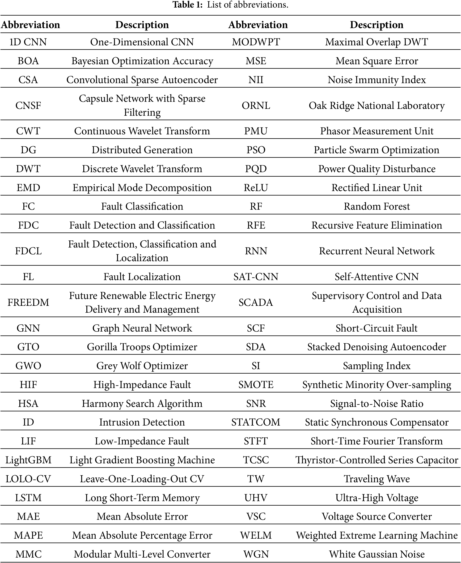
Table 1 lists the abbreviations and acronyms used throughout this paper for quick reference.
One of the main challenges in using the concept of data-driven artificial intelligence (AI) in fault diagnosis lies in the scarcity of the data itself, owing to the constraints on the availability of fault data in the real world due to privacy and security concerns. Hence, standardized simulation models, which have been well-accepted in the power system field, offer a controlled environment to generate a wide range of fault conditions, thereby providing comprehensive fault data considering the diversity in fault types and system complexities for the purpose of validation [8].
The proposed study is developed and validated using a MATLAB/Simulink-based high-fidelity 735 kV, 32-bus UHV transmission grid system [9]. In power system research, real-time measurements are often scarce and not publicly available owing to security and privacy concerns related to critical infrastructure. Access to hardware-in-the-loop platforms and dedicated real-time simulators is limited in several research environments. Therefore, simulation-based frameworks are widely accepted and provide a controlled and reproducible environment for systematic fault diagnosis analysis. Although this study does not employ hardware-in-the-loop or physical real-time simulators, the MATLAB/Simulink-based UHV system captures practical power system dynamics and supports development and evaluation of advanced deep learning frameworks with potential real-time applicability. Here, “real-time” refers to the proposed 1D-CNN model’s ability to perform fast inference on raw time-series data in simulation without computationally expensive signal processing. The framework remains consistent with established practices and supports reproducibility and future real-time deployment. Although various methodologies [10–12] have been shown to have high accuracy and fast learning capabilities, end-to-end processing is essential. This approach relies on the One-Dimensional Convolutional Neural Network (1D CNN) and evaluates the accuracy, computation time, and memory consumption, which are very critical factors in the development of current technologies.
Most of the previously used techniques [13,14] prove to be accurate enough in fault diagnosis, but they highly rely on the preprocessing stages that involve image transformation techniques, making them impossible to use in real-time monitoring because of the complexity of calculations. On the other hand, the suggested technique provides an extensive analysis of computation time at each step of the processing procedure [15–17], which is usually omitted in previous works [18].
Classical and advanced optimization classifiers [12,19–22] rely on handcrafted feature engineering for effective learning, which requires domain expertise and may discard discriminative temporal and spectral information embedded in raw fault signals. As power system complexity increases, designing features that generalize across diverse fault scenarios can become increasingly challenging, limiting model scalability and robustness. Moreover, hybrid fault ride-through strategies can improve the overall resilience and operational feasibility of next-generation power systems such as HVDC transmission systems [23].
Although the methodologies [24–26] show efficient model learning using numerical or transformed data from Simulink standard models, further optimization in the feature extraction phase is necessary to ensure the efficiency of the end-to-end processing. Moreover, although the proposed methodologies [1,15,27] show high noise immunity, they use noise cancellation techniques, which increase the computational cost. However, the existing methodologies face difficulties in processing high noise levels of 10–20 dB [28–30]. Improving noise immunity may require sophisticated noise-cancellation or denoising techniques, which can increase computational complexity and hinder real-time deployment. The proposed work uses the nominal sampling frequency and investigates the impact of the sampling frequency on fault signal processing. Moreover, the proposed work eliminates the need for high sampling frequencies [8,31], which usually range from 0.2 to 10 MHz. Prior research [19,27,32,33] indicates combined voltage-current (VI) signals outperform individual voltage or current signals, though VI signals remain susceptible to downsampling effects, underscoring the need for optimal sampling frequency selection.
For optimizing the model learning, Bayesian optimization (BO) is employed, which is more efficient than traditional grid and random search methods [34]. Although the efficiency of some techniques has been shown to improve the performance of fault diagnosis, such as the use of harmony search and particle swarm optimization algorithms for parameter tuning and classifier co-training, it has been argued that these approaches are computationally costly and there exists a trade-off [26,35,36]. In the proposed research study, the scalability and adaptability of the fault diagnosis system will be assessed by taking into consideration a large-scale UHV power system with compensation systems. This is because scalability and adaptability are important considerations that enable the fault diagnosis system to handle increasing data patterns and fault complexities.
The proposed methodology overcomes the challenges in fault diagnosis in large-scale series-compensated UHV power systems by utilizing the proposed 1D CNN model with Bayesian optimization. This facilitates efficient processing without the need for intensive pre-processing. The computational resources required for the proposed approach are analyzed to provide a balance between efficiency and accuracy. The simulation models employed in the suggested method enable thorough validation of the approach. This method enhances adaptive fault diagnosis systems for UHV power systems.
The study makes the following key contributions for large-scale UHV power systems:
• End-to-end learning with a 1D CNN enables the autonomous extraction of optimal features from raw fault signals in time-series form, eliminating the need for manual feature engineering.
• The convolutional model minimizes memory requirements and achieves consistent execution speed irrespective of system complexity, thus improving the efficiency of computation.
• Inclusion of Bayesian optimization enables efficient model learning compared to conventional parameter tuning techniques, thus improving the efficiency of the model.
• In-depth analysis of the efficiency of computation time, memory usage, noise immunity, and sampling rate effects enables a scalable approach for real-time fault diagnosis in large series-compensated UHV systems.
In [1], a Self-Attentive Weight-Sharing Capsule Network (WSCN) has been proposed to ensure accurate fault diagnosis in series-compensated transmission lines using robust classification with limited data and highlighting the features using weight sharing. In [2], a lightweight CNN fine-tuned with energy valley optimizer was designed using Continuous Wavelet Transform (CWT) scalograms, achieving superior fault diagnosis performance compared to benchmark architectures on balanced, unbalanced, and noisy datasets. This research in [3] introduced an RF-LSTM-tuned KNN ensemble that achieved 99.96% accuracy for fault detection and classification by analyzing voltage and current patterns across transmission line phases.
In [4], empirical mode decomposition extracts features from voltage and current waveforms to train an Extreme Gradient Boost classifier, achieving 97.59% accuracy for incipient fault identification in underground cables. In [5], an Autogluon-based machine learning method for fault diagnosis in transmission lines showed how important feature engineering and the Minority Over-sampling Technique (SMOTE) data balance were to improving diagnostic accuracy. In [6], a graph autoencoder-based detector with bi-level optimization was developed for false data injection attacks on voltage regulation, achieving a 98.11% detection rate on the 486-bus Iberian power system.
In [7], three deep recurrent neural network (RNN) models using Long Short-Term Memory (LSTM) and Phasor Measurement Unit (PMU) data were introduced for fault region identification, type classification, and location prediction, achieving superior accuracy in a two-area four-machine system. In [8], a traveling wave (TW)-based fault location method was proposed combining time- and frequency-domain features, achieving low estimation error across the IEEE 34-node system feeder length.
In [10], a Wide Neural Network (WNN) was presented using PMU voltage, current magnitude, and phase angles for fault location on the Western Systems Coordinating Council (WSCC) 9-bus system, achieving low prediction errors.
This article [11] proposed a fault classification algorithm using Maximal Overlap Discrete Wavelet Packet Transform (MODWPT) and a bagged tree ensemble for Thyristor-Controlled Series Capacitor (TCSC)-compensated transmission lines, achieving 100% accuracy on the WSCC 9-bus system. In [12], a Particle Swarm Optimization (PSO)-weighted ensemble method was presented for real-time fault detection using raw data, validated on IEEE 14-bus and 39-bus systems without pre-computational techniques. The study [13] proposed a CNN with Gorilla Troops Optimizer (GTO) adaptive protection scheme for the Future Renewable Electric Energy Delivery and Management microgrid, achieving 99.37% fault detection, 99% classification, and 98.2% location accuracy.
In [14], a data reduction method using Short-Time Fourier Transform (STFT) and Fast-DTW was proposed to reduce redundant data by 40.2% before CNN training. The approach achieved 99.37% fault classification accuracy in simulations. In [15], SAT-CNN (self-attention CNN) along with time-series images was introduced to classify faults in transmission lines. This model gave high accuracy in the presence of both voltage and current data at different sample rates.
A machine learning approach for transmission line fault detection and location has been proposed in [16]. XGB obtained a classification accuracy of 99.82%, whereas the MAPE of CNN-LSTM is less than 1% and the mean absolute error (MAE) is less than 0.16 km. In [17], a deep learning method using a CNN was proposed for power quality disturbance (PQD) diagnosis. It classified fault types and locations with over 99% accuracy using 50 Hz simulated data.
In [18], three deep learning models (CNN, LSTM, and CNN-LSTM) were proposed for smart grid fault diagnosis on IEEE 6-bus and 9-bus systems. They outperformed existing methods in detection, classification, and localization accuracy. In [19], four ensemble classifiers were evaluated for fault diagnosis on series-compensated power transmission lines (SC-PTL). RF achieved 99.94% accuracy, while XGB showed the fastest computation at 0.2790 s. In [20], an ML-based intrusion detection framework was proposed for Supervisory Control and Data Acquisition (SCADA) power systems using the Oak Ridge National Laboratory (ORNL) dataset. RF achieved a 94.09% F1 score on unseen data after augmentation and balancing.
In [21], eight classifiers were evaluated for fault classification using a standardized Simulink dataset. Logistic Regression (LR), RF, and Support Vector Machines (SVM) outperformed others with high accuracy and reduced computational time. In [22], A hybrid framework combining 21 domain-knowledge features with machine learning was proposed for transmission line fault diagnosis. XGB achieved 94.25% accuracy across 11 fault categories. In [24], an SA-MobileNetV3 model with CWT-based 2D image conversion was proposed for transmission line fault classification. It achieved 99.90% accuracy across 11 fault types.
In [25], Power System Machine Learning (PSML), an open-access multi-scale time-series dataset for joint transmission and distribution grids, was presented to enable ML-based reliable grid operation and decarbonization research. In [27], A SAT-CNN with DWT denoising and time-series imaging was proposed for transmission line fault classification. It achieved high accuracy and noise immunity. In [28], a transfer learning method using a Stacked Denoising Autoencoder (SDA) was proposed for Voltage Source Converter High-Voltage Direct Current (VSC-HVDC) fault location. It performed effectively with small datasets under various fault conditions.
In [29], fuzzy thresholding, machine learning with wild horse optimization, and adaptive neural fuzzy inference were proposed for smart grid fault diagnosis. RF achieved 100% accuracy with
In [32], a capsule network with sparse filtering (CNSF) was proposed for unsupervised fault detection and classification in transmission lines. It performed effectively under topology changes, noise, and high-impedance faults (HIF). In [33], a Convolutional Sparse Autoencoder (CSA) was proposed for transmission line fault detection and classification. The system automatically learned its features and showed good robustness and generalizability. According to [34], an LSTM model along with DWT-based feature extraction was used to find HVDC faults. This method was capable of achieving an accuracy of 99.04% with a fault resistance of 480 ohms and using a three-level relay system
The hybrid method using ANN along with RF with the help of the Optuna optimization technique was proposed in [36] for fault diagnosis in electrical power networks. Using Synthetic Minority Over-sampling Technique (SMOTE)-balanced data, the model was able to obtain an accuracy of 99.8%, outperforming other traditional and advanced classifiers. However, challenges exist regarding computational efficiency and practical validation. In [37], a unified multi-task learning framework with an attention mechanism and Optuna optimization achieved high-accuracy fault identification, classification, and localization on the IEEE 39-bus system, outperforming traditional models. In [38], an intelligent relaying scheme was proposed using Variational Mode Decomposition (VMD)-extracted current signal features and a CNN classifier for fault diagnosis in Doubly-Fed Induction Generator Unified Power Flow Controller (DFIG-UPFC) transmission lines, achieving fast fault detection (
A robust CNN-BFO architecture was proposed in [39] for PV fault identification based on the integration of five CNNs (GoogleNet, SqueezeNet, ResNet-50, VGGNet-16, and AlexNet) and Bitterling Fish Optimization (BFO) for selection. VGGNet-16+BFO achieved 98.75% accuracy, 98.72% sensitivity, 98.78% specificity, 98.76% precision, and 98.74% F1 score, outperforming other meta-heuristic optimizers. The study in [40], performed fault analysis of UHV power systems via simulation-based fault diagnosis. The methods of feature engineering and ensemble learning were used to get accurate results for fault detection and localization.
The issue of fault detection in series-compensated ultra-high voltage transmission lines continues to be difficult in spite of notable progress made through the use of artificial intelligence. Earlier studies have demonstrated classification accuracies higher than 99% on a wide range of power systems of different levels of complexity. However, there are some constraints associated with these methods, which restrict their implementation in real-time applications to large-scale series-compensated power systems. These methods utilize many complex pre-processing algorithms such as HSA, DWT, CWT, EMD, MODWPT, and image-based signal processing methods. For instance, the hybrid machine and deep learning frameworks reported in [3,16,40] required processing times of 10,920, 2712.80, and 840 s, respectively, to achieve optimal performance. These substantial computational requirements, together with significant memory demands, may limit their suitability for real-time protection applications.
Moreover, the test and validation of existing methodologies in small or medium-sized systems like IEEE 4-bus, 6-bus, 9-bus, and 14-bus systems, without using series compensation and operating at UHV levels, does not show the scalability of these methodologies under real-world system scenarios. The reliance on engineered features and transformation from signal to images can lead to a loss of valuable time data present within the transient fault signals, as well as increased computational overhead, rendering it impractical for implementation. Signal ablation studies have not been sufficiently carried out, resulting in an inability to determine the efficiency of diagnosis if partial data from sensors is unavailable. Scalability in terms of sensitivity to various sampling rates from 1 to 100 MHz and signal-to-noise ratio of 20 dB shows performance deterioration to around 97% precision. Many current methodologies do not adequately report inference times, training times, memory requirements, and their ability to generalize fault classifications for multiple fault resistances and series-compensated networks.
Therefore, these challenges highlight the critical necessity of an efficient and effective end-to-end fault diagnostic model able to process unprocessed multivariate discrete-time data directly without any computationally expensive feature extraction step. This model has to achieve accurate diagnostics while significantly lowering the preprocessing costs, making sure to attain efficient and effective training and inference with the possibility of implementing real-time operation, and at the same time exhibiting good performance even under signal masking and noise injection, as well as varying sample rates, in large series-compensated UHV transmission systems. In order to tackle the aforementioned problems, this study introduces a Bayesian-optimized One-Dimensional Convolutional Neural Network fault diagnostic framework, which learns discriminative features directly from the raw signal measurements with emphasis on accurate fault diagnostics, efficient computation, robustness, and potential real-time deployment.
This paper is organized as follows: The next Section 2 discusses the proposed framework for the Bayesian-optimized one-dimensional convolutional neural network. This includes dataset pre-processing or signal de-interleaving, a one-dimensional convolutional neural network for feature extraction, classification and optimization, performance metrics, and lastly the dataset used for the experiment. The experimental findings and their corresponding discussion are presented in Section 3. This includes accuracy and efficiency analysis, Bayesian optimization and learning, performance generalization and overfitting characteristics, noise analysis, sampling analysis, the perfect recipe or the optimized hyperparameters identified by the Bayesian optimization algorithm, comparison with existing work, and lastly the future scope. The last Section 4 discusses the conclusion.
2 Proposed Bayesian-Optimized 1D CNN Framework
The proposed methodology for multi-class fault classification involves three main stages: (1) Dataset structuring via signal de-interleaving, (2) Model development using a Bayesian-optimized 1D Convolutional Neural Network (CNN), and (3) Performance evaluation.
Fig. 1 shows a fault classification pipeline using a 1D CNN with leakage prevention. Raw signals are preprocessed to a fixed length before train/test splitting. Training involves normalization on the training dataset; Bayesian optimizations are done only using the training dataset, with the hyperparameters optimized using standard 10-fold cross-validation and hyperparameter evaluation. Convolution, pooling, depthwise blocks, global attention, and softmax functions are used in the model for classification purposes. Test datasets are kept separate with normalized values and one-off evaluations. Results include accuracy, confusion matrix, and classification report, maintaining strict train-test separation while optimizing performance.
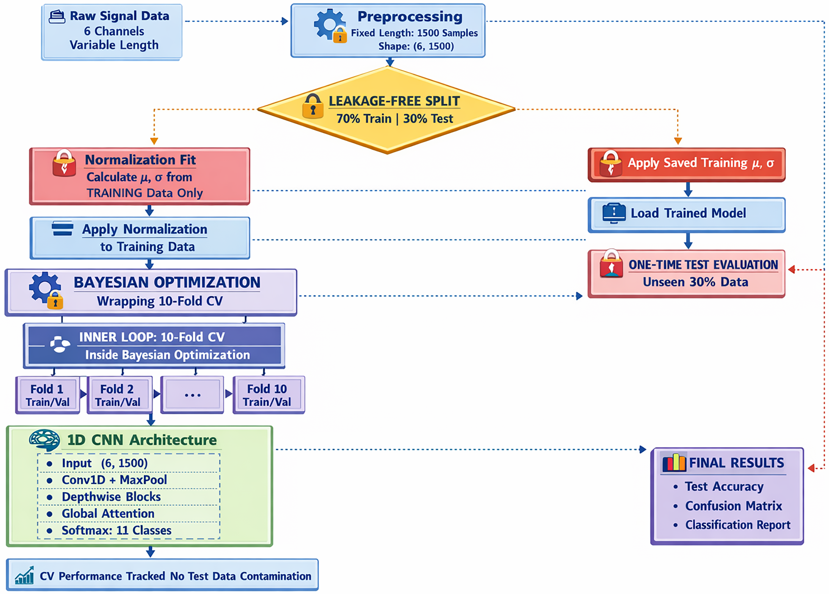
Figure 1: Leakage-aware 1D CNN fault classification pipeline with Bayesian optimization and 10-fold cross-validation in a series-compensated power transmission grid system.
2.1 Dataset Preprocessing: Signal De-Interleaving
The raw dataset is a composite matrix,
Let the raw data matrix be
For a system with
De-interleaving is the process of reshaping each row of signals into a structured 2D format suitable for a 1D CNN. Specifically, a raw signal vector
2.2 1D Convolutional Neural Network for Feature Extraction
A 1D CNN is employed to automatically learn salient features from the de-interleaved fault signals. The core operation is the 1D convolution. Given an input signal
where
To reduce dimensionality and extract dominant features, a max-pooling layer is applied. For a pooling size
After several convolutional and pooling layers, the extracted high-level features are flattened into a 1D vector
2.3 Classification and Optimization
The final layer of the network is a dense layer with 11 neurons, employing the softmax activation function to produce a probability distribution over the 11 classes. For an input feature vector
The model is trained by minimizing the categorical cross-entropy loss. For a single training sample with true class label
2.4 Hyperparameter Optimization Using Bayesian Optimization
To automate and optimize the network’s architecture and training hyperparameters (e.g., number of filters, kernel size, learning rate, number of layers), Bayesian Optimization is employed. The aim is to identify the hyperparameter configuration
Bayesian optimization uses a probabilistic model of the objective function, typically a Tree-Structured Parzen Estimator or a Gaussian Process. It uses an acquisition function for optimization, which efficiently searches for the optimal set of hyperparameters by intelligently selecting the next set of hyperparameters to evaluate, thus being more efficient than grid or random search.
The optimized model’s performance is assessed through various metrics:
• Cross-Validation Accuracy: The average accuracy obtained using the 10-fold cross-validation technique over the training data, which is used as the objective function
• Test Accuracy: The accuracy of the trained model over the test data.
• Training Time: The time taken to train the model with the optimized hyperparameters.
• Bayesian Optimization Time: The time taken to finish the hyperparameter optimization process.
• Memory Usage: The memory used during the training process.
• Classification Report and Confusion Matrix: Calculated over the test data to obtain the precision, recall, and F1-score for each of the 11 classes (10 fault types + 1 normal condition), along with the visualization of the confusion matrix.
Analysis of the sampling frequency is important in fault classification since the fidelity of the signal is dependent on the sampling rate; failure to sample sufficiently can cause high-frequency fault information to be lost. The test setup produces multivariate fault signals having a sampling frequency of 20 kHz. In order to study the influence of the sampling frequency on fault detection, the signal is down-sampled from 1 to 15 kHz. This down-sampling is done under different operating conditions and fault transitions in order to systematically analyze the influence of sampling frequency on fault detection.
Noise tolerance is important in simulated fault detection since noise can affect the signals of power systems in the process of measuring, communicating, and through sensors. Simulating the model under various noise conditions tests how well the model performs. White Gaussian noise is used to simulate signals with SNRs varying between 10 and 50 dB.
The discrete-time fault signal
In this context,
The process ensures that the noise introduced corresponds to the given SNR, thus enabling a systematic analysis of fault detection under noisy conditions.
The experimental setup, as depicted in Fig. 2, is implemented in Simulink, which simulates a modern power transmission grid at 735 kV, along with a Modular Multi-Level Converter (MMC)-based STATCOM. This consists of 22 sub-modules per arm, which are delta-connected via an 18/735 kV transformer. By adjusting the voltage level of the converter relative to the grid, one can achieve different modes: the inductive mode occurs when the voltage is lower, whereas the capacitive mode happens when the voltage is higher.
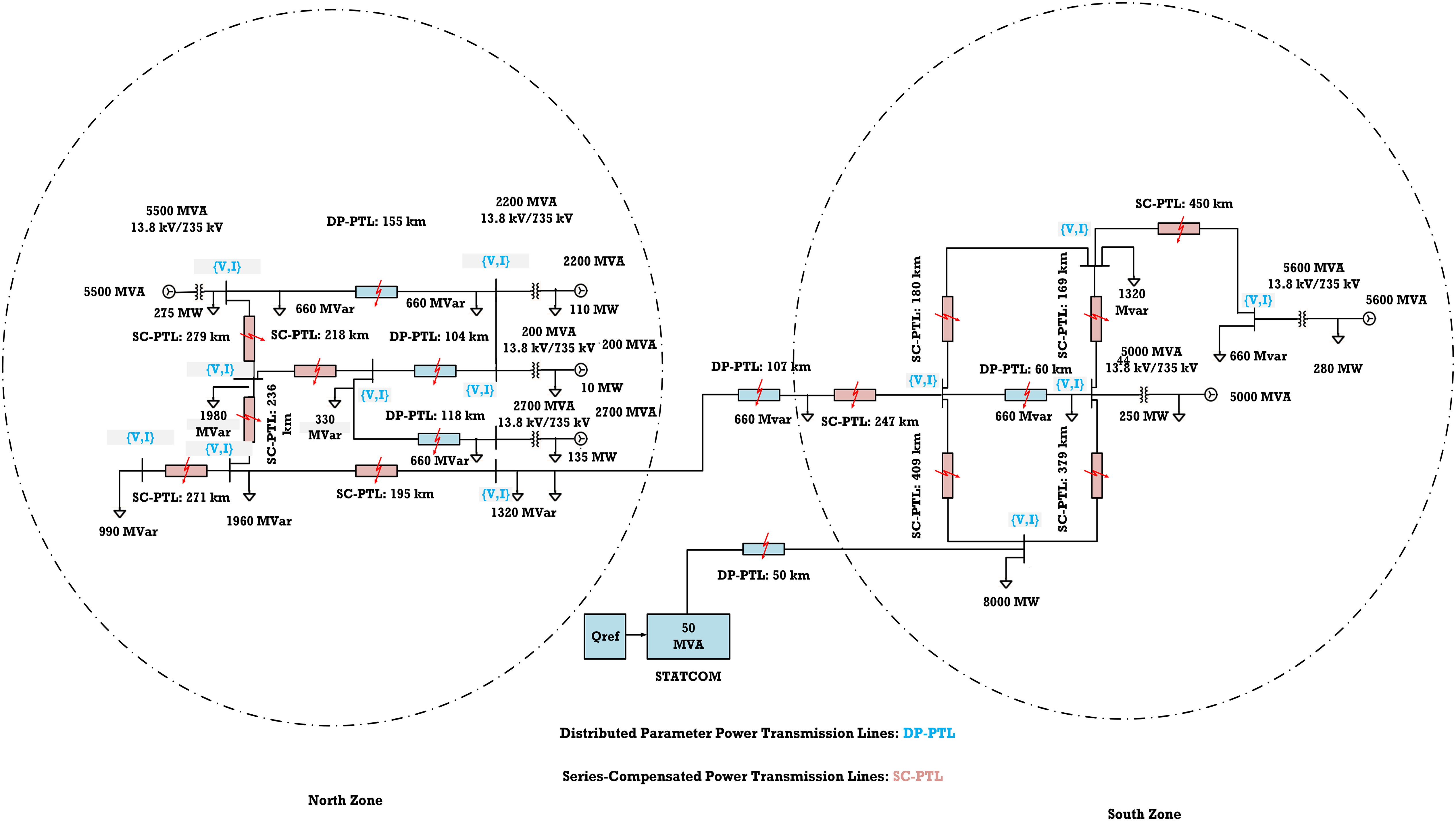
Figure 2: Single-line diagram of the 735 kV power transmission grid system, illustrating the North and South zones with generation capacities, line lengths, load distributions, and the MMC-STATCOM location.
The simulated system represents a 60 Hz, 32-bus network with six generating stations, multiple transformers, shunt elements, and 17 distributed parameter transmission lines, of which 11 are series-compensated (15%–42%) to enhance the power transfer capability. A 50 MVA STATCOM is included for voltage regulation and stability support. For a complete understanding of the implementation, one can refer to [9], which thoroughly describes the high-fidelity operation of a physical UHV power system.
For data generation, simulations are conducted for 0.5 s at a 20 kHz sampling frequency (corresponding to
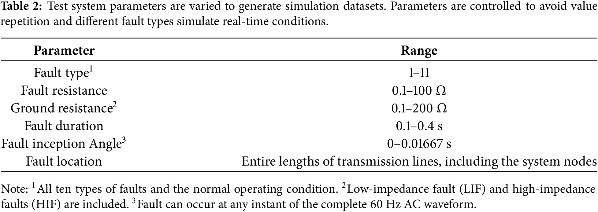
Furthermore, faults are applied on the entire network, including transmission lines and buses, enabling system-wide analysis. This strategy improves the overall dataset diversity and can be effective in assessing the scalability of the proposed methodology based on the complexity of faults in large-scale UHV power systems. The fault signals are collected from all the main system buses to obtain fault data. This data recording scheme is essential for efficient fault diagnosis within power systems since the placement of PMUs in a power system is significant for efficient analysis, as discussed in [10]. Table 2 shows the parameters used for simulation purposes. The parameters are varied based on randomized non-repeating numbers for efficient simulation results. This strategy ensures unique fault simulation (no duplications) based on dynamic operating conditions within power systems.
Algorithm 1 outlines the process of creating a labeled dataset of short-circuit fault signals with the help of a Simulink UHV power grid model by varying the fault parameters randomly over
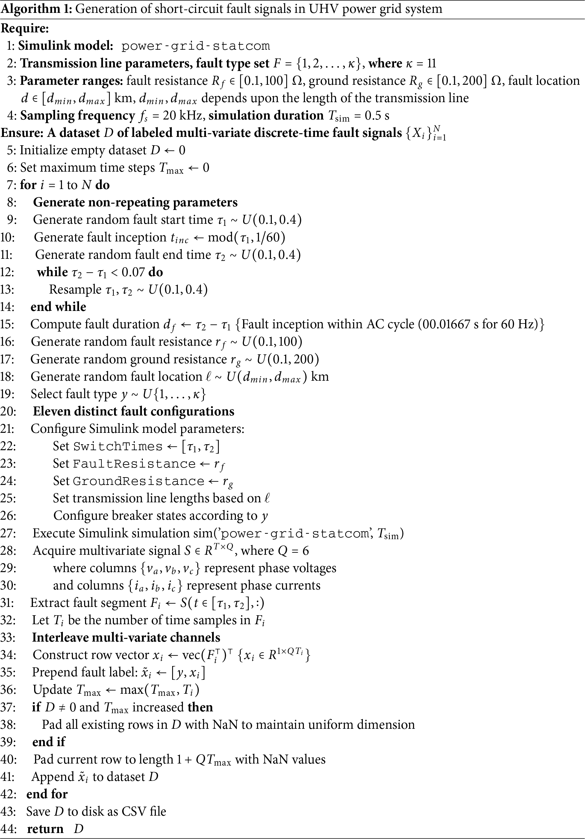
For the sake of consistent length, all the samples are padded with NaN and stacked vertically into the dataset
Fig. 3 shows the waveforms used for the generation of the datasets in time-series format, illustrating various dynamic operating conditions such as system oscillations, equipment saturation, and nonlinear dynamics in the power grid system. These datasets simulate complex behaviors such as system oscillations and non-linearities, which affect the fault signatures under realistic operating scenarios. These datasets help to validate the diagnostic tool by subjecting it to various fault conditions, thus improving the potential and ability of the tool to diagnose faults comprehensively.
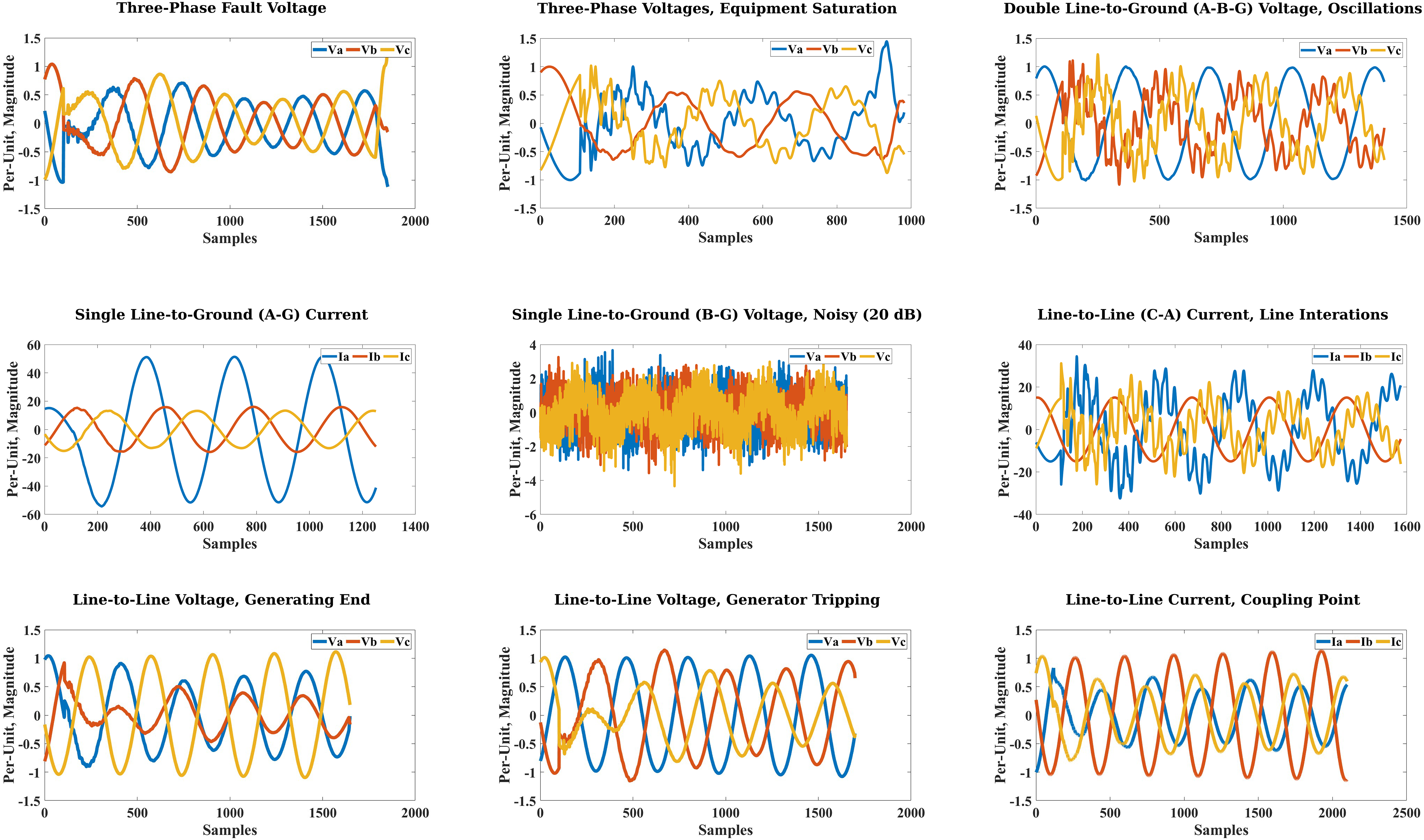
Figure 3: Representative three-phase voltage and current waveforms illustrating diverse fault conditions, including oscillations, saturation, noise effects, and line interactions in power system dynamics.
3.1 Accuracy and Efficiency Analysis
The performance analysis in Fig. 4a indicates that all three signal configurations have fault classification accuracy above 99%. Among the three, the voltage-current scheme has the highest performance with 99.91% test accuracy and the least standard deviation of
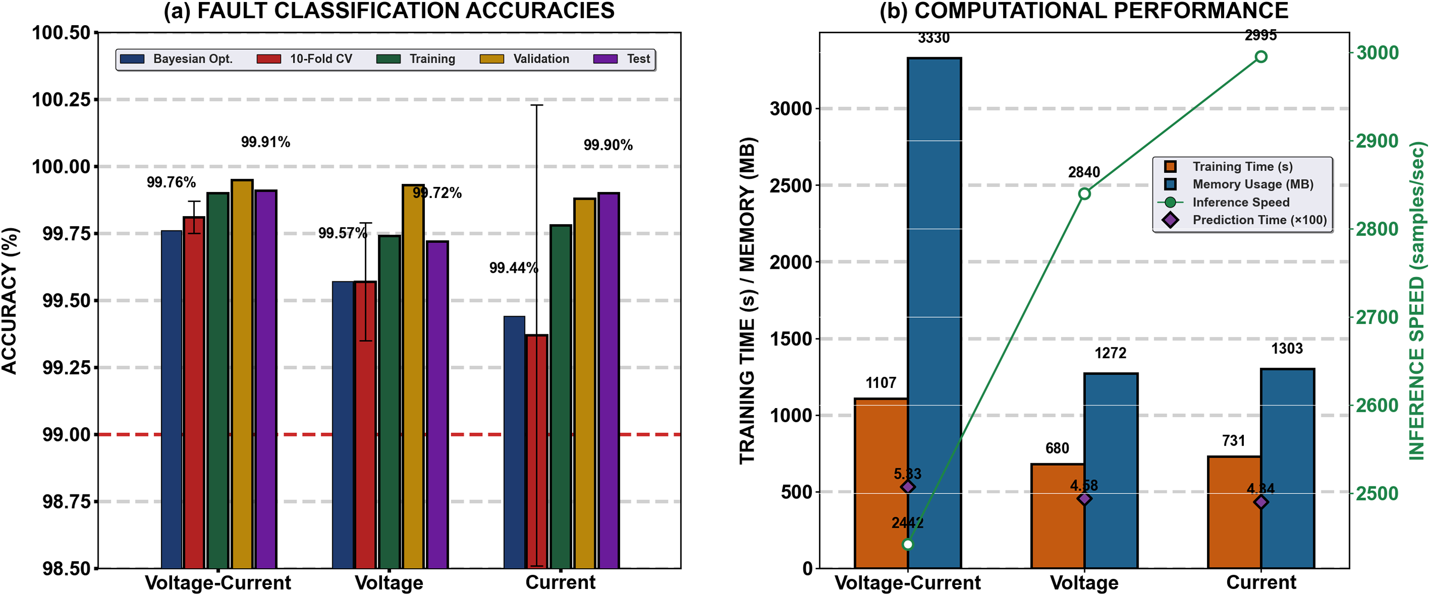
Figure 4: Performance comparison of signal types for UHV fault classification. (a) Accuracy metrics showing all models
As can be seen in Fig. 4b, these methods have clear trade-offs between accuracy and computational efficiency. The voltage-current model is recommended for critical fault diagnosis systems where maximum accuracy is required; the voltage-only model is the best choice for edge computing scenarios where resources are limited; while the current-only model is the best option for high-frequency monitoring where real-time response is required. As can be seen, the viability of the three modalities of the signal is verified in the above analysis.
3.2 Bayesian Optimization and Model Learning
The Bayesian optimization process achieved a best cross-validation accuracy of 99.76% at the twelfth iteration for the VI signals, as shown in Fig. 5a. The corresponding configuration used a learning rate of 0.002611, dropout rate of 0.182, batch size of 19, and weight decay of
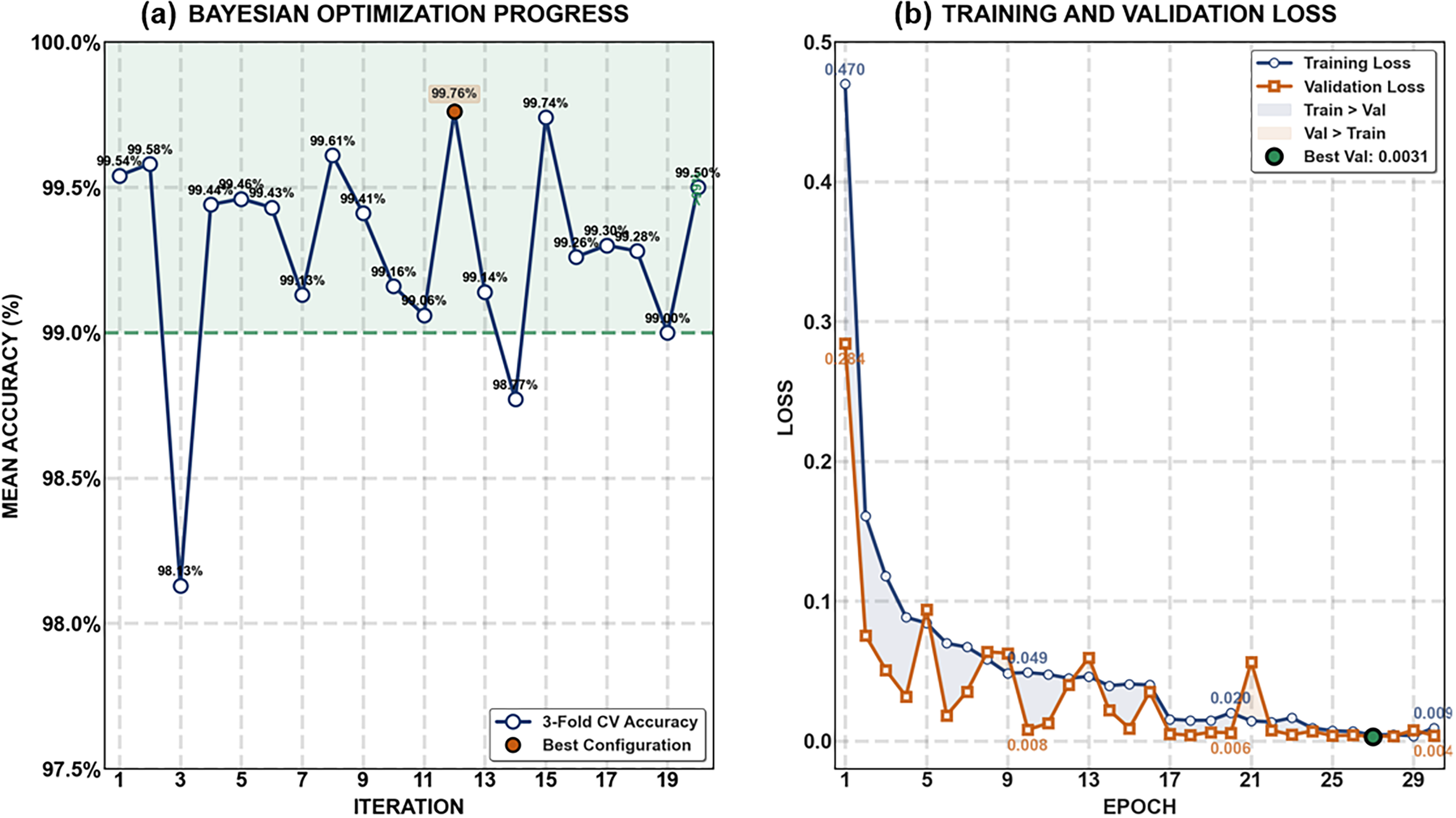
Figure 5: Optimization and training performance. (a) Bayesian optimization over twenty iterations achieves 99.76% peak accuracy at iteration twelve (orange), with most configurations exceeding 99% (green region). (b) Training and validation loss curves over thirty epochs show the best validation loss of 0.0031 at epoch twenty-seven (green point).
The proposed architecture contains 913,314 trainable parameters, providing sufficient capacity to learn complex patterns associated with the UHV power system configuration. As shown in Fig. 5b, the validation performance improved up to epoch 27, where the validation loss reached 0.0031 and validation accuracy reached 99.95%. The training loss decreased from 0.4698 to 0.0093, corresponding to a 98% reduction, while the model achieved a training accuracy of 99.72% at the final epoch. After epoch 27, the validation loss increased slightly to 0.0038, and validation accuracy decreased marginally to 99.92% at epoch 30. This small degradation indicates a minor decline in validation performance during the final training epochs and suggests the onset of overfitting, although the final validation accuracy remained high. The training–validation accuracy difference at the final epoch was
3.3 Feature Representation and Discriminative Capability Analysis
The outcomes of feature analysis also show the representation learning process of the proposed neural architecture. As illustrated in Fig. 6, the ratio of sparsity increased gradually from the shallow to deep layers of the network, reaching over 0.84 in conv3, global_ctx1, global_ctx3 and fc1. It can be seen from the observation that the deeper layers were able to learn more selective feature representations as a result of removing redundancy from the features while keeping the discriminative fault information intact. At the same time, the positive weight ratios stayed relatively well-balanced at about 0.5 for most layers, implying stable feature learning without any notable bias towards positive or negative kernel responses.
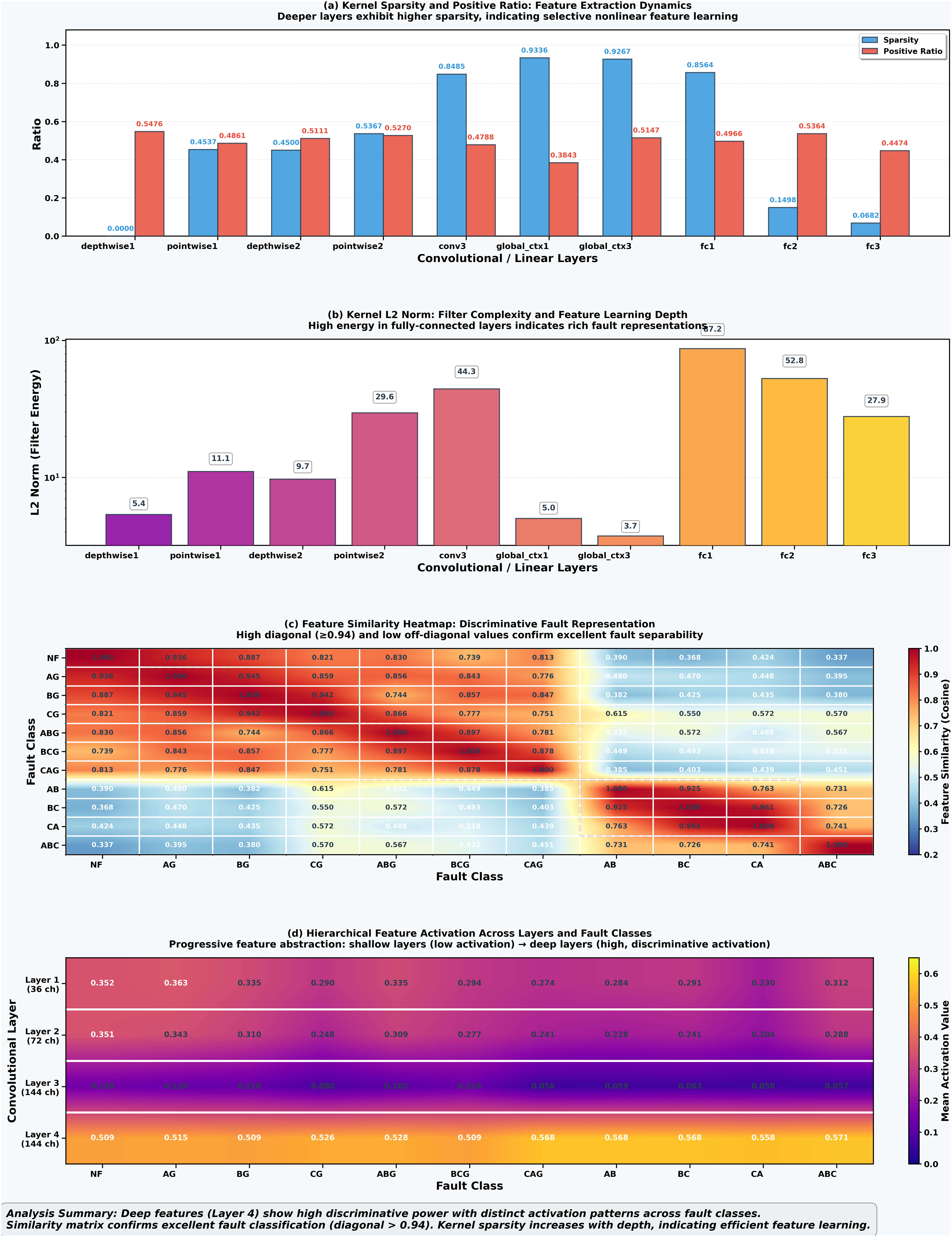
Figure 6: Analysis of learned representations in the proposed 1D CNN model: (a) kernel sparsity and positive-weight ratios, (b) kernel L2 norms, (c) inter-class feature similarity heatmap, and (d) layer-wise feature activations, demonstrating progressive feature abstraction and effective fault-class discrimination.
The kernel energy analysis showed that the L2 norms increased noticeably in the deeper layers, especially in the fully connected part of the network, where fc1, fc2, and fc3 reached 87.24, 52.78, and 27.89, respectively. This suggests that these higher-level layers captured more meaningful fault-related patterns and played a stronger role in making the final decision. On the other hand, the global context layers had much smaller L2 norms, which indicates that they mainly acted as lightweight attention modules for refining features rather than directly extracting the main representations.
The matrix of similarity of features indicates that the classifier is able to acquire very coherent features within each fault class while at the same time maintaining a high level of class separability. All diagonal elements of this matrix are greater than 0.86; in some classes, they exceed 0.98, which means that the features within each type of fault form clusters which are very coherent. Simultaneously, the low level of similarity off the diagonal, particularly between uncorrelated fault groups, indicates that the classifier is able to discriminate between classes. This is also evident from the results of class separability, including the Fisher separability index of 2.33 and the high level of between-class scatter relative to within-class scatter.
The hierarchical activation analysis shows how the model gradually learns more meaningful fault features as the data moves deeper through the network. In the first two convolutional layers, the activations are moderate, mainly capturing basic local patterns in the signals. The third layer becomes more selective, with lower overall activation but higher sparsity, meaning it focuses only on the most important features. By the final feature layer, the activations become stronger and more consistent—around 0.51 to 0.57 across different fault classes—showing that the network has successfully converted raw signal information into compact and clearly distinguishable fault representations. The clear differences in activation patterns between fault types further confirm that the model is effectively learning class-specific characteristics needed for accurate diagnosis.
3.4 Perfromance Generalization and Overfitting Characteristics
Fig. 7a showed evaluation on held-out testing data (30% of total samples) demonstrates exceptional performance with 99.9078% accuracy, correctly classifying 12,998 out of 13,010 instances with only twelve misclassifications across eleven fault categories. This further confirms the fact that the model learns discriminative features and is able to effectively transfer them to new examples. As depicted in Fig. 7b, the F1-score for Classes 1, 10, and 11 is perfect with a score of 1.0000. For Classes 2, 4, 7, and 9, the F1-score is above 0.9990, and the errors are spread out over a few categories. This further confirms the fact that the chosen hyperparameters result in a model with a proper bias-variance trade-off, which is essential in real-world applications.
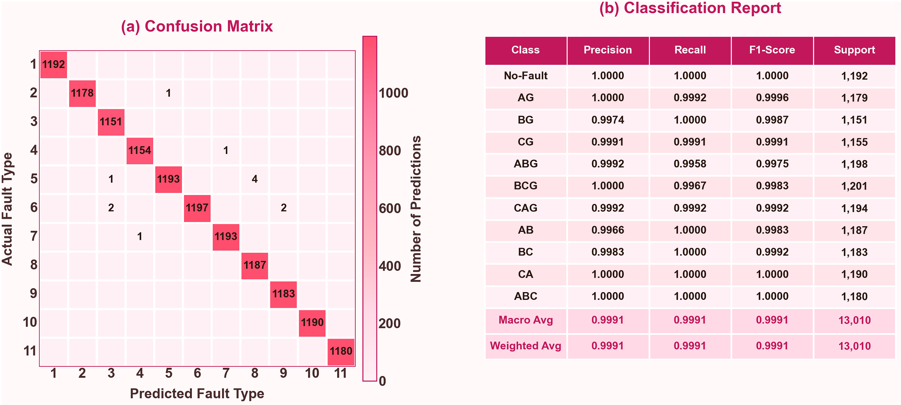
Figure 7: Comprehensive evaluation of the best-performing fault classification model on held-out test data (30% of total samples).
To assess the efficacy of the 1D CNN, noise analysis within a range of 10–50 dB is conducted with VI signals, which confirms the methodology’s noise immunity under noisy conditions. The corruption of fault signals with WGN is an estimate of the methodology’s robustness, as power system sensors are found to show Gaussian-type noise distortion in real-time operating conditions. As shown in Fig. 8a, it is clear that there is strong resilience to all types of noise. The performance of the classifier is found to show significant patterns under high noise conditions. At 10 dB, it is found to show 95.97% cross-validation and 97.03% test accuracy, while at 20 dB, it is found to show 98.27% cross-validation and 98.28% test accuracy. Although there is a small decline in performance at 30 dB, with 97.56% test accuracy, it is clear from the results obtained at 40 and 50 dB, with 99.57% and 99.25% test accuracy, respectively, that there is effective handling of all types of signal-to-noise ratios.
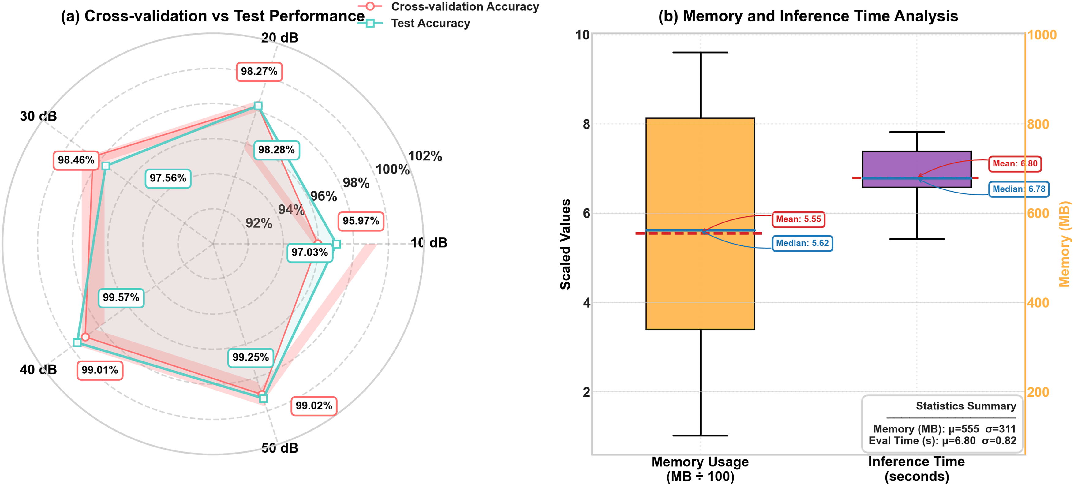
Figure 8: (a) Radar plot showing cross-validation and test accuracy across 10–50 dB noise levels, with error bands indicating standard deviation. (b) Box plot showing memory usage and inference time distribution with mean (red dashed) and median (blue solid) alignment indicating stable performance.
In Fig. 8b, memory usage varies between 102.11 MB for 50 dB and 959.97 MB for 40 dB. The average memory usage is 555 MB, while the median is 562 MB. This shows symmetry in memory usage for all the noise levels. The average inference time is 6.80 s, while the median is 6.78 s. The standard deviation for inference time is 0.82 s. This shows consistent performance in real-time processing. The classifier shows high immunity to all levels of noise. This eliminates the need for computationally expensive methods for noise cancellation or heavy preprocessing as reported in [1,24]. The accuracy for all levels of noise is above 97.03%, even for the highest noise level of 10 dB.
However, the similarity of mean and median for memory usage and inference time does not prove a normal distribution of the data but shows similar central tendencies among the analyzed conditions. Variations of memory usage and inference time show how the computational needs change in various noise levels. However, the classifier has demonstrated very good accuracy under different noise levels, that show consistency of the fault diagnosis process. Thus, these findings serve as proof of the robust fault pattern recognition by the classifier under the analyzed conditions. Comprehensive assessment across a broader range of operating conditions, noise levels, system configurations, and real-world scenarios would be required to further validate generalization, scalability, and deployment performance in critical-infrastructure environments.
The Noise Immunity Index (NII), defined in (8), provides a standardized quantitative measure of model robustness against noise by considering the classification performance across the entire investigated SNR range rather than only the extreme operating conditions. A lower NII indicates greater immunity to noise and more stable performance under varying operating environments.
where
The NII is calculated as
This methodology is tested with voltage-only (V), current-only (I), and combined VI signals at various frequencies (1–20 kHz). The performance of the signals has been presented in Fig. 9, where the performance of the VI signals has been the most consistent. The performance of the signals has reached 99.81 ± 0.06% cross-validation accuracy and 99.91% test accuracy at 20 kHz. The performance of the voltage-only signals has reached 99.92% test accuracy at 5 kHz with 99.69 ± 0.15% cross-validation accuracy. The performance of the current-only signals has reached 99.90% test accuracy at 20 kHz with 99.37 ± 0.86% cross-validation accuracy.
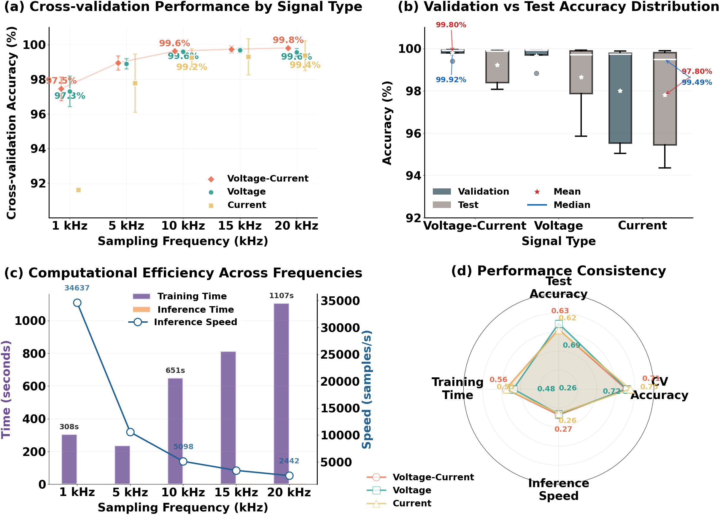
Figure 9: Performance metrics vs. sampling frequency: (a) Cross-validation accuracy, (b) Accuracy distribution, (c) Computational efficiency, (d) Normalized performance radar. V-I signals demonstrate optimal balance across all metrics.
As shown in Fig. 9c, for current-only signals, the training time is the least at 400.3 s compared to VI signals at 623.6 s and voltage-only signals at 545.6 s. Current-only signals have a reduction of 60% compared to VI signals. For inference speed, voltage-only signals have the highest at 14,213 samples per second, followed by current-only signals at 14,124 samples per second, and then VI signals at 11,228 samples per second. Current-only signals have the least memory footprint, while voltage-only and VI signals are moderate. The optimal accuracy-efficiency balance is between 5 and 15 kHz. As shown in Fig. 9d, for VI signals, there is consistent performance in terms of accuracy and efficiency for fault classification.
The proposed methodology is flexible in terms of sampling rates used in fault signals. It can reduce the computational load of data processing devices. The proposed methodology overcomes the limitations of the existing methodologies in terms of the range of sampling frequency used in the signals of the complex power system. The accuracy of the learning algorithms is generally decreased with the downsampling process. However, in the proposed methodology, it is observed that the effects of the downsampling process between the frequency range of 5–20 kHz on the VI signals are less significant. The proposed methodology is satisfactory even at the frequency of 1 kHz. The reason is that the recording of the fault signals is obtained at different locations in the power system in the proposed methodology, which provides more fault information. Despite the loss of information in the significant downsampling process, the proposed methodology is more computationally efficient in the fault diagnosis of the power system compared with the existing methodologies that require the sampling frequency of 10–100 MHz.
The Sampling Index (SI), defined in (9), evaluates the sensitivity of the proposed approach to variations in sampling frequency by considering the entire investigated sampling range.
where
3.7 The Perfect Recipe: Optimized Hyperparameters from Bayesian Optimization
As presented in Table 3, the optimized hyperparameters obtained via the application of the Bayesian optimization approach show the flexibility of the approach in adapting to the conditions of the analysis scenario. For the analysis scenario of the preliminary condition, the optimized parameters are determined to be batch size = 19, learning rate = 0.002611, dropout rate = 0.182, weight decay =
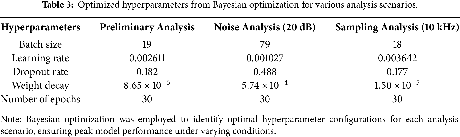
For sampling analysis with a sampling rate of 10 kHz, the hyperparameters are similar to those obtained by preliminary analysis, i.e., batch size is set to 18, the learning rate is set to 0.003642, the dropout rate is set to 0.177, weight decay is set to
3.8 Comparison to Existing Work and Future Scope
Table 4 highlights that the proposed 1D CNN framework achieves superior accuracy even when applied to a highly complex UHV power grid configuration, which involves a 735 kV, 32-bus system with extensive compensation and multiple transmission lines. Although most of the currently available solutions may demonstrate high performance in some operational cases, those solutions require complex preprocessing, including the transformation of faults into image representations, thus increasing computational costs and distancing from the initial signal form. In contrast to that, the proposed solution allows classifying faults using the signal level without any additional processing and expert knowledge required.
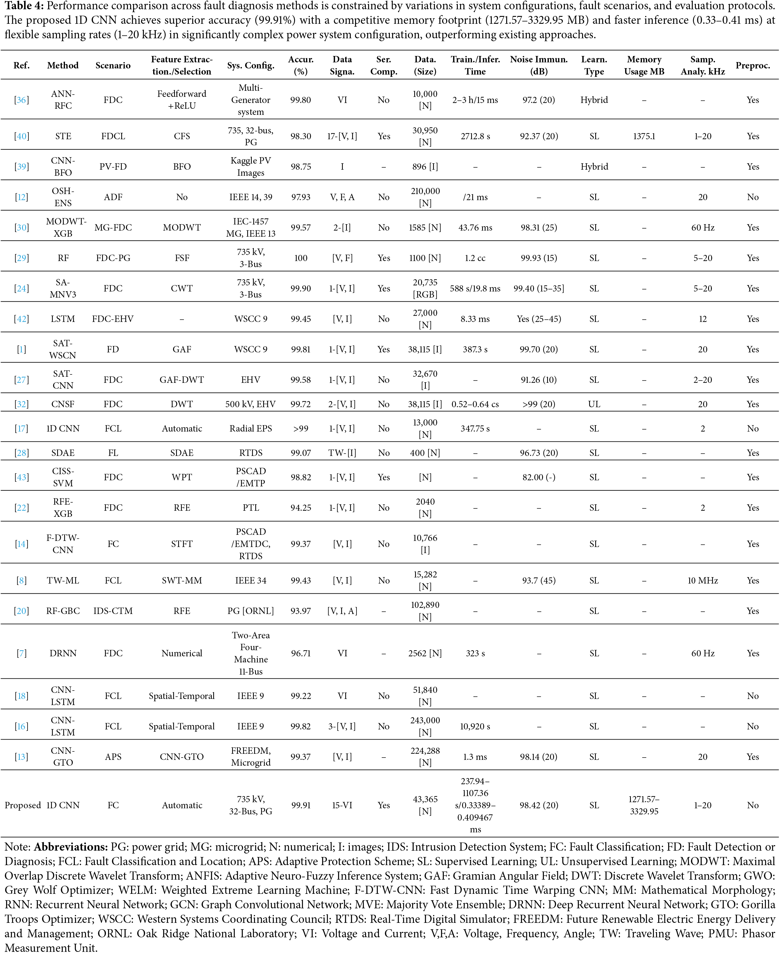
To ensure an unbiased comparison across diverse studies, the framework introduces uniform indices for sampling and noise immunity, allowing performance evaluation under varying data complexities and operating conditions. The results show that the proposed method not only achieves excellent accuracy but also maintains outstanding robustness under noisy environments and downsampling scenarios. Furthermore, it provides a comprehensive analysis across multiple signal types, which is particularly valuable in data-scarce conditions. Unlike most prior works, this study also reports memory usage, revealing that while VI signals demand higher resources, individual voltage or current signals achieve comparable efficiency to existing methods, making the approach adaptable depending on resource constraints. Importantly, the framework challenges fault classification in UHV systems by incorporating a system-wide analysis across all transmission lines, thereby enhancing generalization and scalability compared with studies limited to specific lines.
By replicating the complexities of a physical UHV system in a simulation, the proposed methodology demonstrates its practical relevance and confirms its potential as a robust solution for fault diagnosis in large-scale power grids.
The proposed study demonstrates the effectiveness of a lightweight 1D CNN classifier for fault classification in UHV power systems, validated using a standard simulation setup operating at UHV level with series-compensated and distributed transmission lines designed by domain experts. The real-time Simulink model replicates the complexities of practical large-scale power systems, ensuring realistic evaluation. The 1D CNN effectively addresses dynamic and challenging operating conditions, delivering high accuracy and computational efficiency through end-to-end learning on raw time-series fault signals, which aligns with modern sensor recordings and eliminates the need for heavy preprocessing or transformations.
The automatic feature engineering capability of the model surpasses traditional methods reliant on sophisticated feature extraction and selection, which may fail to capture the intricate behaviors of series-compensated UHV systems. Bayesian optimization for hyperparameter tuning enhances the robustness and efficiency of model development. The data processing pipeline achieves high noise immunity and mitigates the adverse effects of downsampling, providing operational flexibility for diverse data processing devices.
The introduction of quantitative comparative metrics enables fair evaluation across fault diagnosis methodologies that differ in system configurations, data complexity, and operating conditions. While the method effectively overcomes many limitations, further work is needed to optimize noise cancellation using advanced lightweight filtering and improve memory utilization when handling a large number of synchronous recordings, a common scenario in practical systems. Given its robustness, the proposed approach has potential extensions to intrusion detection and fault localization in power grids.
In summary, this rigorously evaluated methodology establishes a proof of concept for practical, scalable fault diagnosis in large-scale UHV power systems, combining accuracy, efficiency, and adaptability to real-world conditions.
Acknowledgement: The authors extend their appreciation to the Research, Development, and Innovation Authority (RDIA), Saudi Arabia, for funding this work through grant number (13385-Tabuk-2023-UT-R-3-1-SE).
Funding Statement: This article is derived from a research grant funded by the Research, Development, and Innovation Authority (RDIA)—Kingdom of Saudi Arabia—with grant number (13385-Tabuk-2023-UT-R-3-1-SE).
Author Contributions: Hani Albalawi: Conceptualization, methodology, and writing—review and editing; Rab Nawaz: Software, investigation, data curation, and writing—original draft; Abdul Wadood: Conceptualization, validation, supervision, and writing—review and editing; Anwar Ul Haq: Formal analysis, visualization, and validation; Shahbaz Khan: Software, investigation, and data analysis; Bakht Muhammad Khan: Methodology, resources, and writing—review and editing; Aadel Mohammed Alatwi: Project administration, funding acquisition, and writing—review and editing. All authors reviewed and approved the final version of the manuscript.
Availability of Data and Materials: The data that support the findings of this study are available from the Corresponding Author.
Ethics Approval: Not applicable.
Conflicts of Interest: The authors declare no conflicts of interest.
References
1. Fahim SR, Sarker SK, Muyeen SM, Sheikh MRI, Das SK, Simoes M. A robust self-attentive capsule network for fault diagnosis of series-compensated transmission line. IEEE Trans Power Deliv. 2021;36(6):3846–57. doi:10.1109/tpwrd.2021.3049861. [Google Scholar] [CrossRef]
2. Teta A, Korich B, Bakria D, Hadroug N, Rabehi A, Alsharef M, et al. Fault detection and diagnosis of grid-connected photovoltaic systems using energy valley optimizer based lightweight CNN and wavelet transform. Sci Rep. 2024;14(1):18907. doi:10.1038/s41598-024-69890-7. [Google Scholar] [CrossRef]
3. Anwar T, Mu C, Yousaf MZ, Khan W, Khalid S, Hourani AO, et al. Robust fault detection and classification in power transmission lines via ensemble machine learning models. Sci Rep. 2025;15(1):2549. doi:10.1038/s41598-025-86554-2. [Google Scholar] [CrossRef]
4. Sahoo PK, Mishra S, Swain SC. Classification of incipient fault in underground distribution networks using extreme gradient boost classifier. In: Proceedings of the 2025 International Conference on Power Electronics and Energy (ICPEE); 2025 Dec 14–16; Bhubaneswar, India. New York, NY, USA: IEEE; 2025. p. 1–6. [Google Scholar]
5. Demirci M. Multi fault classification in electrical transmission lines using feature engineering based on autogluon framework. Sustain Comput Inform Syst. 2026;50(15):101310. doi:10.1016/j.suscom.2026.101310. [Google Scholar] [CrossRef]
6. Fahim SR, Atat R, Kececi C, Takiddin A, Ismail M, Davis KR, et al. Graph neural network-based approach for detecting false data injection attacks on voltage stability. IEEE Open J Power Energy. 2025;12:12–23. doi:10.1109/oajpe.2024.3524268. [Google Scholar] [CrossRef]
7. Belagoune S, Bali N, Bakdi A, Baadji B, Atif K. Deep learning through LSTM classification and regression for transmission line fault detection, diagnosis and location in large-scale multi-machine power systems. Measurement. 2021;177(3):109330. doi:10.1016/j.measurement.2021.109330. [Google Scholar] [CrossRef]
8. Jimenez-Aparicio M, Wilches-Bernal F, Reno MJ. Local, single-ended, traveling-wave fault location on distribution systems using frequency and time-domain data. IEEE Access. 2023;11:74201–15. doi:10.1109/access.2023.3296737. [Google Scholar] [CrossRef]
9. Series-compensated transmission system—MATLAB & Simulink—mathworks.com. [cited 2026 Mar 5]. Available from: https://www.mathworks.com/help/releases/R2024b/sps/ug/power-grid-statcom.html. [Google Scholar]
10. Yuvaraju V, Thangavel S, Golla M. Applications of artificial intelligence and PMU data: a robust framework for precision fault location in transmission lines. IEEE Access. 2024;12(6):136565–87. doi:10.1109/access.2024.3464088. [Google Scholar] [CrossRef]
11. Mishra PK, Yadav A. Fault classification scheme for TCSC compensated transmission line using MODWPT-BTEC. e-Prime Adv Electr Eng Electron Energy. 2024;9:100729. doi:10.1016/j.prime.2024.100729. [Google Scholar] [CrossRef]
12. Yavuz L, Soran A, Önen A, Li X, Muyeen S. Adaptive fault detection scheme using an optimized self-healing ensemble machine learning algorithm. CSEE J Power Energy Syst. 2021;8(4):1145–56. doi:10.17775/cseejpes.2020.03760. [Google Scholar] [CrossRef]
13. Hatata AY, Essa MA, Sedhom BE. Adaptive protection scheme for FREEDM microgrid based on convolutional neural network and Gorilla troops optimization technique. IEEE Access. 2022;10:55583–601. doi:10.1109/access.2022.3177544. [Google Scholar] [CrossRef]
14. Yang NC, Yang JM. Fault classification in distribution systems using deep learning with data preprocessing methods based on fast dynamic time warping and short-time Fourier transform. IEEE Access. 2023;11:63612–22. doi:10.1109/access.2023.3288852. [Google Scholar] [CrossRef]
15. Fahim SR, Sarker MRI, Arifuzzaman M, Hosen MS, Sarker SK, Das SK. A novel approach to fault diagnosis of high voltage transmission line-a self attentive convolutional neural network model. In: Proceedings of the 2020 IEEE Region 10 Symposium (TENSYMP); 2020 Jun 5–7; Dhaka, Bangladesh. New York, NY, USA: IEEE; 2025. p. 1329–32. [Google Scholar]
16. Minh NQ, Khiem NT, Giang VH. Fault classification and localization in power transmission line based on machine learning and combined CNN-LSTM models. Energy Rep. 2024;12(1):5610–22. doi:10.1016/j.egyr.2024.11.061. [Google Scholar] [CrossRef]
17. Yoon DH, Yoon J. Deep learning-based method for the robust and efficient fault diagnosis in the electric power system. IEEE Access. 2022;10:44660–8. doi:10.1109/access.2022.3170685. [Google Scholar] [CrossRef]
18. Alhanaf AS, Farsadi M, Balik HH. Fault detection and classification in ring power system with DG penetration using hybrid CNN-LSTM. IEEE Access. 2024;12:59953–75. doi:10.1109/access.2024.3394166. [Google Scholar] [CrossRef]
19. Nawaz R, Wadood A, Khalid Mehmood K, Basit Ali Bukhari S, Albalawi H, Mohammed Alatwi A, et al. Gradient boosting feature selection for integrated fault diagnosis in series-compensated transmission lines. IEEE Access. 2025;13:63640–70. doi:10.1109/access.2025.3558796. [Google Scholar] [CrossRef]
20. Zaman M, Upadhyay D, Lung CH. Validation of a machine learning-based IDS design framework using ORNL datasets for power system with SCADA. IEEE Access. 2023;11:118414–26. doi:10.1109/access.2023.3326751. [Google Scholar] [CrossRef]
21. Nawaz R, Albalawi HA, Ali Bukhari SB, Khalid Mehmood K, Sajid M. Timeseries fault classification in power transmission lines by non-intrusive feature extraction and selection using supervised machine learning. IEEE Access. 2024;12(4):93426–49. doi:10.1109/access.2024.3423828. [Google Scholar] [CrossRef]
22. Guo B, Yang B, Wang S, Shi W, Yang F, Wang D. Machine learning-based fault diagnosis and classification of three-phase transmission lines with RFE and domain knowledge. Electr Power Syst Res. 2025;247(2):111777. doi:10.1016/j.epsr.2025.111777. [Google Scholar] [CrossRef]
23. Liu K, Li B, Jiang Q, Zhang Y, Liu T. Fault ride-through strategy for hybrid cascaded HVDC systems based on controllable LCC. IEEE Trans Circuits Syst II. 2026;73(1):88–92. doi:10.1109/tcsii.2025.3627209. [Google Scholar] [CrossRef]
24. Xi Y, Zhang W, Zhou F, Tang X, Li Z, Zeng X, et al. Transmission line fault detection and classification based on SA-MobileNetV3. Energy Rep. 2023;9:955–68. doi:10.2139/ssrn.4226448. [Google Scholar] [CrossRef]
25. Zheng X, Xu N, Trinh L, Wu D, Huang T, Sivaranjani S, et al. A multi-scale time-series dataset with benchmark for machine learning in decarbonized energy grids. Sci Data. 2022;9(1):359. doi:10.1038/s41597-022-01455-7. [Google Scholar] [CrossRef]
26. Xu W, Li J, Yang L, Yu Q. Faults locating of power distribution systems based on successive PSO-GA algorithm. Sci Rep. 2024;14(1):11259. doi:10.1038/s41598-024-61306-w. [Google Scholar] [CrossRef]
27. Fahim SR, Sarker Y, Sarker SK, Sheikh MRI, Das SK. Self attention convolutional neural network with time series imaging based feature extraction for transmission line fault detection and classification. Electr Power Syst Res. 2020;187(5):106437. doi:10.1016/j.epsr.2020.106437. [Google Scholar] [CrossRef]
28. Shang B, Luo G, Li M, Liu Y, Hei J. Transfer learning-based fault location with small datasets in VSC-HVDC. Int J Electr Power Energy Syst. 2023;151:109131. doi:10.1016/j.ijepes.2023.109131. [Google Scholar] [CrossRef]
29. Najafzadeh M, Pouladi J, Daghigh A, Beiza J, Abedinzade T. Fault detection, classification and localization along the power grid line using optimized machine learning algorithms. Int J Comput Intell Syst. 2024;17(1):49. doi:10.1007/s44196-024-00434-7. [Google Scholar] [CrossRef]
30. Patnaik B, Mishra M, Bansal RC, Jena RK. MODWT-XGBoost based smart energy solution for fault detection and classification in a smart microgrid. Appl Energy. 2021;285:116457. doi:10.1016/j.apenergy.2021.116457. [Google Scholar] [CrossRef]
31. Almeida AR, Almeida OM, Junior BFS, Barreto LHSC, Barros AK. ICA feature extraction for the location and classification of faults in high-voltage transmission lines. Electr Power Syst Res. 2017;148:254–63. doi:10.1016/j.epsr.2017.03.030. [Google Scholar] [CrossRef]
32. Fahim SR, Sarker SK, Muyeen SM, Das SK, Kamwa I. A deep learning based intelligent approach in detection and classification of transmission line faults. Int J Electr Power Energy Syst. 2021;133(4):107102. doi:10.1016/j.ijepes.2021.107102. [Google Scholar] [CrossRef]
33. Chen K, Hu J, He J. Detection and classification of transmission line faults based on unsupervised feature learning and convolutional sparse autoencoder. IEEE Trans Smart Grid. 2016;9(3):1748–58. doi:10.1109/pesgm.2017.8273992. [Google Scholar] [CrossRef]
34. Yousaf MZ, Singh AR, Khalid S, Bajaj M, Kumar BH, Zaitsev I. Bayesian-optimized LSTM-DWT approach for reliable fault detection in MMC-based HVDC systems. Sci Rep. 2024;14(1):17968. doi:10.1038/s41598-024-68985-5. [Google Scholar] [CrossRef]
35. Abdelgayed TS, Morsi WG, Sidhu TS. A new harmony search approach for optimal wavelets applied to fault classification. IEEE Trans Smart Grid. 2016;9(2):521–9. doi:10.1109/tsg.2016.2555141. [Google Scholar] [CrossRef]
36. Uzel H, Özüpak Y, Alpsalaz F, Aslan E. Optimized ANN-RF hybrid model with optuna for fault detection and classification in power transmission systems. Sci Rep. 2025;16(1):1495. doi:10.1038/s41598-025-31008-y. [Google Scholar] [CrossRef]
37. Alam MS, Islam MR, Fan R, Alam Shazid MS, Hasan AS. Attention-guided multi-task learning for fault detection, classification, and localization in power transmission systems. Energies. 2025;18(24):6547. doi:10.3390/en18246547. [Google Scholar] [CrossRef]
38. Biswas S, Nayak PK, Panigrahi BK, Pradhan G. An intelligent fault detection and classification technique based on variational mode decomposition-CNN for transmission lines installed with UPFC and wind farm. Electr Power Syst Res. 2023;223(3):109526. doi:10.1016/j.epsr.2023.109526. [Google Scholar] [CrossRef]
39. Sabati A, Bayindir R, Rahebi J. Photovoltaic panels fault detection with convolutional neural network and bitterling fish optimization (BFO) algorithm. Int J Comput Intell Syst. 2025;18(1):239. doi:10.1007/s44196-025-00984-4. [Google Scholar] [CrossRef]
40. Nawaz R, Qamar A, Wadood A, Albalawi H. Consensus-based feature selection and Bayesian-optimized stacking ensembles for comprehensive fault diagnosis in series-compensated ultra-high-voltage power systems. Sci Rep. 2026;16(1):18678. doi:10.1038/s41598-026-49195-7. [Google Scholar] [CrossRef]
41. Ukwuoma CC, Cai D, Bamisile O, Chukwuebuka EJ, Favour E, Emmanuel GSA, et al. Power transmission system’s fault location, detection, and classification: pay close attention to transmission nodes. Int J Electr Power Energy Syst. 2024;156(6):109771. doi:10.1016/j.ijepes.2023.109771. [Google Scholar] [CrossRef]
42. Rafique F, Fu L, Mai R. End to end machine learning for fault detection and classification in power transmission lines. Electr Power Syst Res. 2021;199(10):107430. doi:10.1016/j.epsr.2021.107430. [Google Scholar] [CrossRef]
43. Kumar VR, Jeyanthy PA. Fault classification and detection in transmission lines by hybrid algorithm associated support vector machine. Trans Emerging Tel Tech. 2025;36(3):e70034. doi:10.1002/ett.70034. [Google Scholar] [CrossRef]
Cite This Article
 Copyright © 2026 The Author(s). Published by Tech Science Press.
This work is licensed under a Creative Commons Attribution 4.0 International License , which permits unrestricted use, distribution, and reproduction in any medium, provided the original work is properly cited.
 Downloads
 Citation Tools
