EPITIME: A Computational Framework for Integral Epidemic Models with Structure-Preserving Discretizations

1  Introduction

Mathematical epidemiology has long relied on compartmental models to describe the spread of infectious diseases, with SIR- and SEIR-type systems providing a standard framework for the analysis of transmission dynamics, threshold quantities and control strategies [1,2]. However, several epidemiologically relevant mechanisms, including infection-age dependence, variable infectiousness and memory effects, are more naturally represented within integral formulations than through finite-dimensional compartmental systems alone [3]. Integral models replace constant transition rates with infectivity kernels, allowing for a more general representation of how infectiousness evolves over the course of the disease and naturally incorporating distributed delay effects, such as those induced by incubation and latency periods.

In this context, Brauer and coauthors [1] provided a comprehensive treatment of Age of Infection (AoI) epidemic models, clarifying their analytical properties and their connections to standard compartmental systems. Furthermore, Diekmann and collaborators developed a unified renewal-equation framework for epidemic models that systematically incorporates key biological features such as demography, non-permanent immunity and heterogeneous infectivity. Within this setting, the Force of Infection (FoI), that is the rate at which susceptibles become infected, is expressed through a scalar renewal equation driven by an infectivity function. Classical compartmental models are recovered as particular limiting cases [4,5].

In parallel, increasing attention has been devoted to epidemic models that account for behavioural adaptation, where transmission is affected not only by biological factors but also by changes in human behaviour driven by information, perceived risk, or epidemic awareness [6]. In this setting, integral formulations are particularly natural, since both infection-age effects and behavioural responses can be described through history-dependent terms and distributed kernels. This perspective is especially relevant for information-dependent epidemic models, in which transmission is modulated by an information index reflecting the effect of past epidemic trends on present contact behaviour [7–10].

The numerical approximation of integral epidemic models poses several challenges, especially when one aims to preserve crucial qualitative features of the continuous dynamics, such as positivity, boundedness, invariant regions, equilibrium structure and long-time behaviour. In epidemiological applications, the loss of these structural properties may lead to spurious numerical behaviour and unreliable long-time simulations. For this reason, Non-Standard Finite Difference (NSFD) methods and other structure-preserving discretization techniques have become increasingly relevant in the numerical analysis of epidemic models [11–13]. Appropriately constructed NSFD schemes can retain selected dynamical properties of the underlying continuous problem for arbitrary time steps, under the assumptions associated with each scheme.

Several numerical approaches have been developed for epidemic models with memory, including methods for delay differential equations, distributed-delay and integro-differential equations, fractional-order models and age-structured PDEs. Structure-preserving discretizations have also been proposed for delayed compartmental models, including NSFD schemes designed to retain positivity, boundedness, equilibria and stability or global-dynamics properties [14,15]. Distributed-delay and integro-differential problems can be addressed by direct quadrature and collocation methods [16], as well as by fast convolution techniques designed for evolution equations with memory [17,18]. Alternatively, reduction approaches may approximate the memory kernel by sums of exponentials or related expansions, thereby transforming the distributed-delay term into an enlarged ODE or DDE system [19]. A related but distinct line of research concerns fractional epidemic models, where memory effects are represented by nonlocal derivative operators. In this context, wavelet-based and related high-order methods have been proposed for delayed and piecewise-fractional epidemic dynamics [20,21]. These approaches are particularly relevant when the main objective is the accurate resolution of fractional or delayed fractional dynamics.

Beyond the choice of the numerical discretization, the availability of dedicated software represents a further practical issue. Compartmental epidemic models formulated as Ordinary Differential Equations (ODEs) can rely on widely available and well-established software environments, whereas software for epidemic models governed by integral equations is much less common. This gap is particularly relevant because the specific structure of integral epidemic models, with history-dependent terms, often requires dedicated implementations rather than the direct use of general-purpose solvers.

Several software environments have been developed to support epidemic modelling and simulation. For instance, EpiModel provides an R-based framework for deterministic compartmental, stochastic individual-contact and network epidemic models [22]. Agent- and individual-based epidemic simulation is supported by tools such as Covasim, originally developed for COVID-19 dynamics and intervention analysis [23], and EMOD, a modular individual-based platform for infectious-disease modelling [24]. Spatially explicit and metapopulation epidemic simulations are addressed by frameworks such as GLEAMviz, which combines stochastic epidemic models with global demographic and mobility data [25], and by the Spatiotemporal Epidemiological Modeler (STEM), an open-source environment for spatial and temporal infectious-disease modelling [26,27]. More recently, Epydemix has provided a Python-based framework for the specification, simulation and calibration of stochastic compartmental epidemic models, including demographic structure, contact matrices and Approximate Bayesian Computation tools [28]. Complementary statistical tools also include epidemia, an R package for semi-mechanistic Bayesian modelling of infectious diseases in which transmission dynamics are represented through renewal equations and used for inference, forecasting and scenario analysis [29].

Other computational tools address specific classes of dynamical systems with memory or delay. For example, DDE-BIFTOOL provides MATLAB routines for bifurcation and stability analysis of delay differential equations [30,31]. Similarly, the software collection developed within the CDLab (Computational Dynamics Laboratory), University of Udine, includes tools for the numerical analysis of delay equations and related dynamical systems, such as TRACE-DDE for the computation of characteristic roots and stability charts of delay differential equations [32,33].

Among recent epidemic simulation frameworks, MEmilio is especially relevant to the present work because it explicitly includes integro-differential, or age of infection, epidemic models within a broader multi-model software architecture [34,35]. MEmilio is a modular high-performance framework supporting ODE, integro-differential and agent-based models, together with mobility models and scalable computational implementations. Its IDE-based modelling component has also been developed in connection with NSFD numerical schemes for SECIR-type integro-differential epidemic models with non-exponentially distributed stay times [36].

Despite this broad range of available tools, dedicated computational frameworks for renewal-type integral epidemic models remain comparatively limited. In particular, the software environments discussed above mainly focus on compartmental, network-based, agent-based, individual-based, metapopulation or statistical inference formulations, while general-purpose delay-equation tools are mainly designed for stability, bifurcation or dynamical-systems analysis rather than for the direct simulation of integral epidemic models while preserving their epidemiologically relevant structure.

Motivated by these considerations, this work presents EPITIME (EPidemic Integral models TIMe-profile Explorer), a computational framework for the simulation of two classes of integral epidemic models: an age of infection model and an information-dependent behavioural model. The main focus of the present manuscript is the design and development of a dedicated modular software environment. The continuous epidemic models and the corresponding structure-preserving NSFD discretizations are based on earlier analytical and numerical results. These results are recalled here to provide the mathematical background for the software design and to identify the properties inherited by the implementation.

Compared with broad epidemic simulation environments such as MEmilio, EPITIME has a narrower and complementary scope. It is designed as a dedicated MATLAB/Python framework for selected renewal-type integral epidemic models. Both EPITIME and the IDE component of MEmilio employ structure-preserving non-standard discretizations for history-dependent epidemic dynamics. However, MEmilio implements a detailed SECIR integro-differential model based on transition flows, whereas EPITIME focuses on compact renewal formulations in which the FoI is expressed directly through infectivity kernels.

The MATLAB and Python implementations include input parsing and validation, parameter handling, consistency checks, warning mechanisms and performance indicators to support reproducible numerical experimentation. Furthermore, the interdisciplinary nature of epidemic modelling motivates the development of graphical interfaces that make computational tools accessible to researchers and professionals with diverse scientific backgrounds, including epidemiologists, public-health specialists and policy planners, whose expertise may not extend to the technical aspects of code implementation and numerical analysis. The capabilities of EPITIME are illustrated through representative case studies, including long-time simulations, final-size computations, behavioural dynamics under different memory kernels, and inverse reconstruction of an infectivity kernel from COVID-19 incidence data. Computational performance and scalability are also analysed, with particular attention to history-dependent convolution terms and the implemented truncation strategy. Fast convolution techniques are discussed as a possible future extension.

The paper is organized as follows. Section 2 presents the two epidemic models considered in this work. Section 3 introduces a unifying formulation and reviews the corresponding NSFD discretizations and their main qualitative properties. Section 4 is devoted to the description of the EPITIME software environment, including its MATLAB and Python implementations and the graphical user interface. Section 5 reports a selection of numerical experiments, including tests on asymptotic behaviour, inverse-problem reconstruction and simulations illustrating the qualitative dynamics of the behavioural model. Final remarks are given in Section 6. Two appendices precede the References section, collecting a unified notation guide (Appendix A) and indications on software validation and reproducibility (Appendix B).

2  Model Formulation

In the following sections, two classes of integral epidemic models are considered, distinguishing between formulations in which the FoI depends solely on biological factors and those that explicitly incorporate human behavioural feedback through information-dependent transmission mechanisms.

2.1 The Age of Infection Epidemic Model

The model defined in [1, Chapter 4.5] traces the evolution of an epidemic within a closed population taking into account the cumulative contribution of past infections to the current FoI. The model reads

S′(t)=−β0S(t)φ(t),φ(t)=β0∫0+∞A(τ)S(t−τ)φ(t−τ)dτ,(1)

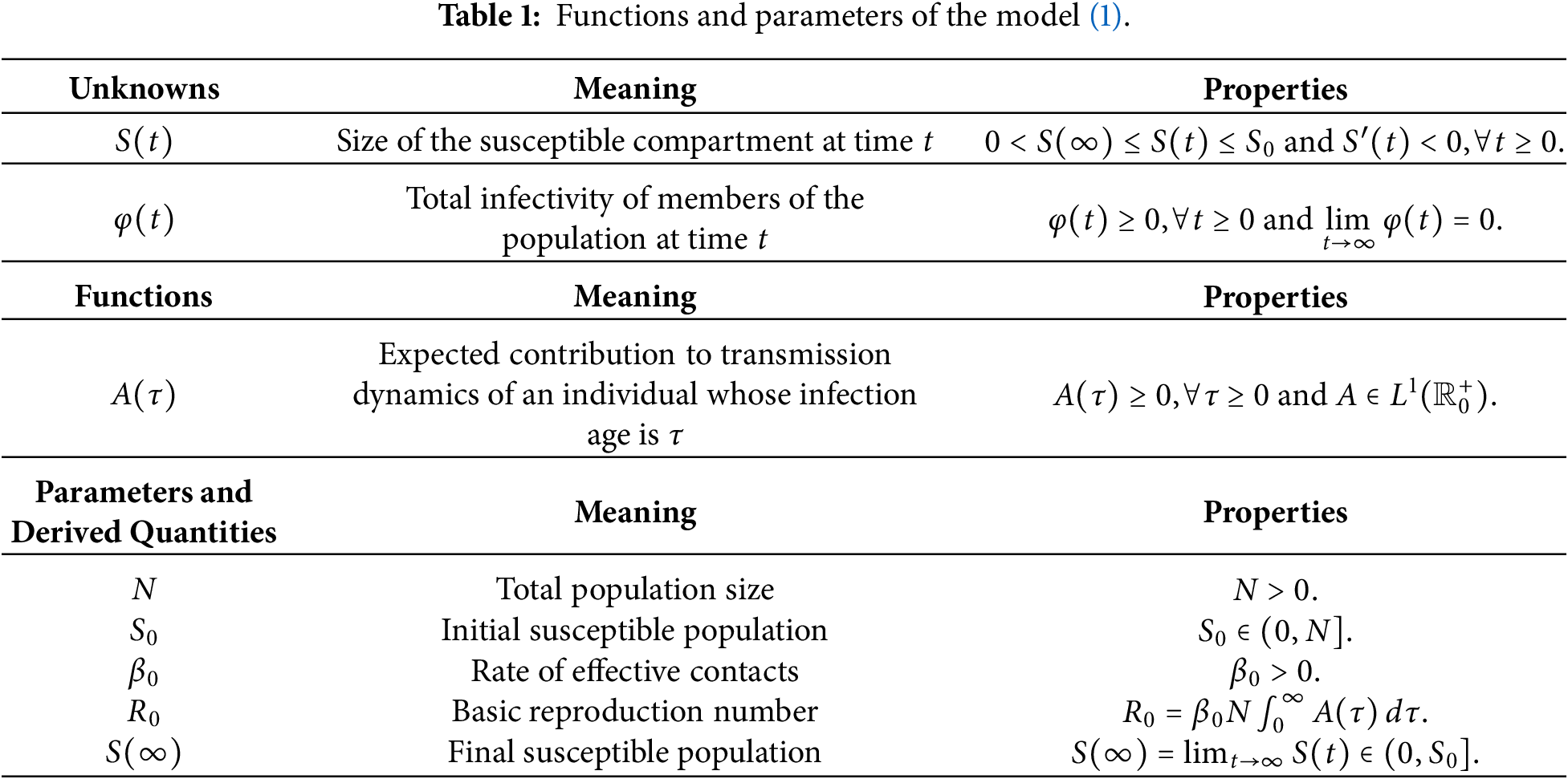
and we refer to Table 1 for a complete description of the variables, parameters and functions.

Here, τ denotes the infection age, that is the time elapsed since the infection. For this reason, from now on, the model (1) is referred to as the “age of infection” (AoI) model. An alternative expression in terms of the FoI is presented in [5], which also explores the connection with compartmental models, and is explored (see Section 9.3 in [37] and Sections 4 and 6 in [38] for further details). Moreover, a broader framework, which incorporates symptomatic and asymptomatic infections [39] as well as heterogeneously mixed populations [40,41], is discussed in [42].

A numerical approximation method for (1), specifically designed to unconditionally preserve selected qualitative properties of the continuous solution, is recalled in Section 3.1. Furthermore, some insights on the asymptotic behaviour of the continuous and numerical solutions to (1) are provided in Section 5.2.

2.2 The Integral Behavioural Epidemic Model

Here, an integral epidemic model is considered that accounts for changes in individual behaviour during an epidemic outbreak by incorporating a time-varying information index M(t). Specifically, this function depends on current and past epidemiological quantities and describes how individuals adjust their risky contacts in response to information and rumours about the disease. The model, whose formulation and analysis are detailed in [8], reads

S′(t)=λ−μS(t)−β(M(t))S(t)F(t),F(t)=∫0∞Aμ(τ)β(M(t−τ))S(t−τ)F(t−τ)dτ,M(t)=∫0∞K(τ)H(t−τ)g(F(t−τ))dτ.(2)

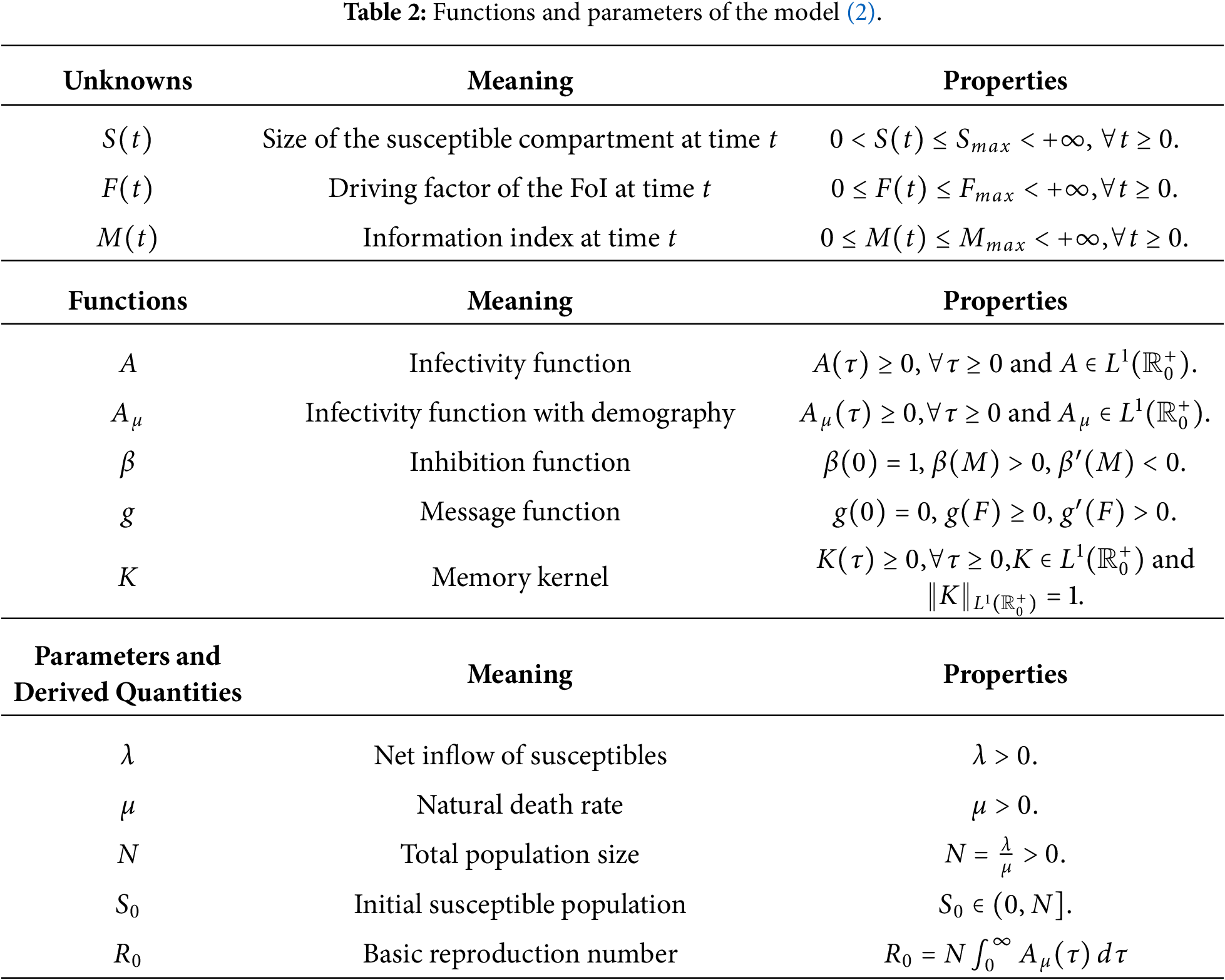
Table 2 provides the unknowns, parameters and known functions of model (2), together with their interpretations and the associated assumptions. Some of the key functions involved are described in more detail in what follows.

In particular, the function Aμ(τ)=e−μτA(τ) describes the infectivity profile over time, where e−μτ accounts for demographic mortality. The inhibition term β(M(t)) captures the reduction in transmission due to information and rumours about the disease. The quantity β(M(t))F(t) represents the FoI at time t. The message function g and the memory kernel K represent the perception of infection risk and how past information influences current behaviour, respectively. Finally, H(⋅) is the Heaviside step function.

Model (2) can be regarded as a natural extension of the work by Breda et al. [4], starting from their formulation and incorporating a dependence of the FoI on the information index. A variant of (2) including incidence–dependent contact patterns is outlined in [9]. There, M(t) is expressed as a weighted sum of past and present contributions of incidence trends, given by kβ(M(t))S(t)F(t), where k∈(0,1) represents the information coverage.

Section 3.2 reviews a numerical approximation technique for model (2) that is specifically constructed to unconditionally preserve selected qualitative properties of its solution.

To improve readability, Appendix A summarizes the main symbols that are used across the two model classes, their discrete counterparts, and the software implementation. Model-specific notation, assumptions and qualitative properties are reported separately in Tables 1 and 2.

3  Solution Methods and Algorithms

To discuss efficient simulation methods for the models introduced in the previous sections, a unifying (d+1)–dimensional framework, which generalizes both (1) and (2), is considered. To this end, we denote by S(t)∈R+ and X(t)=[X1(t),…,Xd(t)]T∈Rd the unknown functions, and by Q(t,τ)∈Rd×d the prescribed kernel of the problem. More specifically, the system

S′(t)=α1−S(t)(α2+G1(X(t))),X(t)=∫0+∞Q(t,τ)G2(S(t−τ),X(t−τ))dτ,(3)

is addressed, where the constants α1,α2∈R0+, and the non-linear functions G1:Rd→R and G2:Rd+1→Rd are given. In particular, the formulations (1) and (2) are recovered from (3) as special cases corresponding to the following choices. For d=1, set α1=α2=0 and:

X(t)=φ(t),Q(t,τ)=A(τ),G1(X)=β0X,G2(S,X)=G1(X)S,

and, for d=2, set α1=λ,α2=μ and:

X(t)=[F(t)M(t)], Q(t,τ)=[Aμ(τ)00H(t−τ)K(τ)], G1(X)=β(X2)X1, G2(S,X)=[G1(X)Sg(X1)],

respectively.

The numerical discretizations presented in the subsequent sections are based on previously developed structure-preserving NSFD methods, which are briefly recalled here to highlight the qualitative properties preserved within the EPITIME software environment. The schemes used in this work exploit the following first-order non-standard approximations of the derivative and integral operators

S′(t+h)≈S(t+h)−S(t)hγ1(h)≈α1−S(t+h)(α2+G1(X(t))),(4a)

∫tt+hQ(t~,t~−τ)G2(S(τ),X(τ))dτ≈hΓ(h)Q(t~,t~−t)G2(S(t+h),X(t)),(4b)

which hold for each fixed t~≥t+h and h>0, with Γ(h)=diag(γ2(h),…,γd+1(h)) and γi(h)=1+𝒪(h),i=1,…,d+1, positive functions. Specifically, Eq. (4a) relies on a weighted forward finite difference, while Eq. (4b) corresponds to a modified rectangular quadrature rule where Q and X are evaluated at the left end-point and S at the right one. This choice is aimed at preserving, independently of the time step-size h, the qualitative properties of the underlying continuous system when passing to a discrete-time formulation. Specifically, positivity, monotonicity and final-size behaviour are retained for the discretization of (1), whereas positivity, boundedness, invariant regions and the equilibrium/threshold structure are preserved by the approximations of (2). The corresponding linearly implicit numerical schemes are derived and discussed in detail in the following sections. Throughout the paper, the assumptions listed in Tables 1 and 2 are understood to hold. Any additional condition needed for the analysis of the numerical asymptotic behaviour will be explicitly stated as required.

3.1 The NSFD Discretization for the Age of Infection Model

Throughout this section, problem (1) is considered and it is assumed that the non-negative function

φ0(t)=β0∫t+∞A(τ)S(t−τ)φ(t−τ)dτ,(5)

is prescribed. As discussed in [43], φ0(t) represents the total infectivity at time t of individuals infected prior to the initial outbreak. In general, it satisfies

0≤φ0(t)≤(N−S0)A(t),(6)

with equality attained when all such individuals have infection age zero at t=0.

Let tn=nh, for n=0,1,…, denote a uniform temporal grid with step-size h>0, and let [Sn, φn]T denote the discrete approximations of the solution to (1) at time tn. The NSFD scheme introduced in [12] is then given by

Sn+1=Sn−hβ0Sn+1φn,φn+1=φ0(tn+1)+hβ0∑j=0nA(tn+1−j)Sj+1φj,(7)

for n=0,1,…, with given initial values S0=S(0) and φ0=φ0(0). The method (7) relies on the non-local approximations outlined in Eqs. (4a) and (4b), with γi(h)=1. Its formulation gives rise to the straightforward linearly implicit update summarized in Algorithm 1.

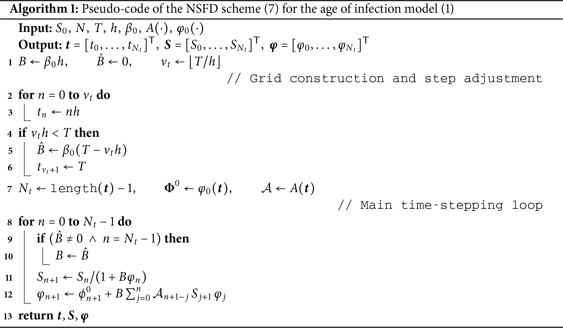
The method (7) belongs to the class of NSFD methods, originally developed for differential equations (see [11] and references therein) and recently extended to integral formulations [13,42]. The following result establishes first-order convergence on finite time intervals. For a detailed error analysis, the reader is referred to Lemma 3.1, Theorems 3.2 and 4.1 in [12].

Theorem 1: Consider problem (1) and assume that A(t)∈C1([0,T]), with 0<t<+∞ and T=n¯h. Denote by E(h;tn)=[S(tn), φ(tn)]T−[Sn, φn]T the global discretization error associated with the NSFD scheme (7). Then,

max0≤n≤n¯‖E(h;tn)‖=𝒪(h),  as h→0.

A key advantage of the NSFD discretization (7) is that it unconditionally preserves the positivity, the monotonicity and the asymptotic behaviour of the continuous solution to (1). These properties, established in Theorem 3.4 in [12] are summarized in the following result.

Theorem 2: Let [Sn, φn]T be the solution to the discrete Eq. (7) with initial values S0>0 and φ0≥0. Then, independently of the step-size h>0, the sequence {Sn}n∈N0 is positive, non-increasing and bounded from above by S0. Therefore, there exists limn→∞Sn=S∞(h)∈(0,S0]. Moreover, {φn}n∈N0 is a non-negative, bounded and vanishing sequence.

3.2 The NSFD Discretization for the Integral Behavioural Epidemic Model

Following the approach and the model formulations presented in [44], to solve the integro-differential system (2), the forcing terms

F0(t)=∫−∞0Aμ(t−τ)β(M(τ))S(τ)F(τ)dτ,M0(t)=∫−∞0K(t−τ)H(τ)g(F(τ))dτ,(8)

are assumed to be given non-negative functions. More precisely, these functions are chosen as suggested in [44]:

F0(t)=Aμ(t)(λ−μS0),M0(t)=g(F(0))K(t).

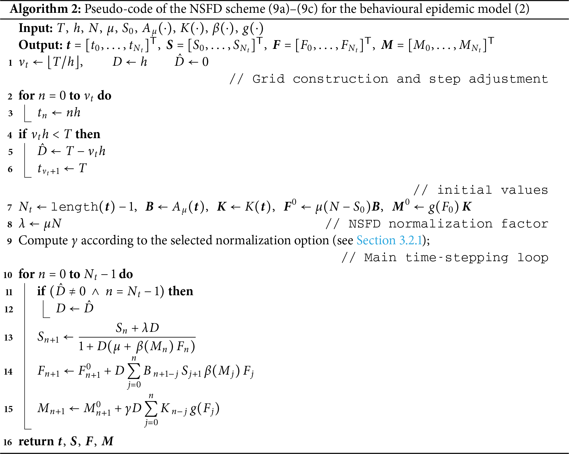
Discretizing the system (2) as detailed in Eqs. (4a) and (4b), with γ1(h)=γ2(h)=1 and γ3(h)=γ(h)=1+O(h) to be specified later, yields the numerical method

Sn+1=Sn+h(λ−μSn+1−β(Mn)Sn+1Fn),(9a)

Fn+1=F0(tn+1)+h∑j=0nAμ(tn+1−j)β(Mj)Sj+1Fj,(9b)

Mn+1=M0(tn+1)+hγ(h)∑j=0nK(tn−j)g(Fj),(9c)

where Sn,Fn and Mn approximate S(tn), F(tn) and M(tn) at the grid point tn=nh, with uniform step-size h>0. Here, the initial values S0=S(0), F0=F(0)=F0(0), and M0=M(0)=M0(0) are given. A pseudo-code of the scheme (9a)–(9c) is presented in Algorithm 2.

A comprehensive analysis of the discrete system (9a)–(9c) is carried out in [44], where the existence and stability of the discrete equilibria are also investigated. In what follows, only a brief overview of these findings is presented, starting from the linear convergence of the method (9a)–(9c).

Theorem 3: Consider the problem (2) and assume that Aμ,K∈C1([0,T]), with 0<t<+∞ and T=n¯h. Denote by E(h;tn)=[S(tn), F(tn), M(tn)]T−[Sn, Fn, Mn]T the global discretization error of the scheme (9a)–(9c). Then,

max0≤n≤n¯‖E(h;tn)‖=𝒪(h),  as h→0.

Assume, in addition to the properties listed in Table 2, that Aμ′(τ),K′(τ)∈L1(R0+) and define, for h∈R+, the functions

A¯μ(h):=h∑n=1∞Aμ(tn),K¯(h):=hγ(h)∑n=0∞K(tn).(10)

Under the above assumptions, the rectangular quadrature rule gives, A¯μ(h)=‖Aμ‖L1(R0+)+𝒪(h) and K¯(h)=‖K‖L1(R0+)+𝒪(h) (see also Lemma 3.3 in [44]). To obtain a structure-preserving discretization which retains the asymptotic behaviour of the solution to (2), we set

γ(h)=1h∑n≥0K(tn).(11)

With this choice the normalization condition K¯(h)=1=‖K‖L1(R0+) is exactly satisfied and γ(h)=1+O(h). Furthermore, the set

D(h)={[x,y,z]T∈R3:0<x≤Smax, 0≤y≤Fmax(h), 0≤z≤Mmax(h)},(12)

is defined, where the upper bounds are given by

Smax=N,Fmax(h)=λ(‖A‖L1(R0+)+A¯μ(h))+N‖Aμ′‖L1(R0+),Mmax(h)=2g(Fmax(h)).(13)

With γ(h) chosen as in (11), the following result holds.

Theorem 4: Suppose that limτ→∞A(τ)=0. Then the region D(h) introduced in (12) is a positively invariant region for the discrete formulation (9a)–(9c).

The discrete model (9a)–(9c) always admits the disease-free equilibrium DFE(h) which corresponds to the extinction of the infection in the population. Moreover, whenever R0(h)>1, with

R0(h)=NA¯μ(h),(14)

and independently of the choice of the kernel K, the system (9a)–(9c) also admits an endemic equilibrium EE(h) (cf. [44, Theorem 4.1]). Remark that R0(h)=R0+𝒪(h) in (14) represents a numerical approximation of the basic reproduction number R0. The stability analysis of EE(h) is based on the linearization theory developed in [45]. Additional details on the topic are provided in [44]. In Section 5.4, numerical examples for selected kernels illustrate the asymptotic behaviour of the solutions of the discrete-time model.

3.2.1 Approximation of the Infinite Discrete Normalization Sum

The exact normalization factor in (11) involves an infinite series. In the current implementation, two alternatives are available for the treatment of the memory normalization, with the choice left to the user. Both options retain first-order consistency. The qualitative properties of the continuous solution are preserved, as detailed in what follows.

Unnormalized option. A straightforward choice is to set γ(h)=1. The main advantage of this option is its reduced computational cost. Its main drawback is the loss of the exact discrete normalization of the memory kernel for fixed h. In this case, the discrete endemic equilibrium depends explicitly on the memory kernel through the factor h∑ℓ=0∞K(tℓ), which enters the relation between the information variable and the force of infection. As a result, both the discrete equilibrium and the associated characteristic equation differ from those obtained with exact discrete normalization by an O(h) perturbation only, provided that the dynamics is sufficiently far from a stability threshold.

Truncated-renormalized option. The infinite series in (11) is replaced by a truncated sum. Specifically, given LK∈N, we set

γLK(h)=(h∑n=0LKK(tn))−1,which implieshγLK(h)∑n=0LKK(tn)=1, ∀h,(15)

assuring the exact discrete normalization. Here, the cutoff index LK is selected so that the neglected discrete tail satisfies

h∑n=LK+1∞K(tn) ≤Ctailh,(16)

for a prescribed constant Ctail>0. This choice ensures that the truncation error induced by the cutoff is of the same order as the time discretization error. Hence, from γLK(h)=1+O(h), the linear convergence of the scheme (9a)–(9c) is retained. Furthermore, since the values K(tn) are non-negative for each n and γLK(h)>0, the qualitative properties of the scheme, such as positivity and boundedness, are preserved independently of h.

The computational cost of this strategy depends on the shape of the memory kernel and, in particular, on its decay rate, since non-monotone or slowly decaying kernels generally require larger values of LK. On the other hand, the exact discrete normalization preserves the discrete equilibrium relations of the continuous model and, consequently, the associated stability properties.

Condition (16) is the theoretical requirement ensuring that the neglected discrete tail is of the same order as the time-discretization error. In the implementation, this condition is approximated by the practical block criterion described below, which is used as a heuristic stopping rule. In practice, the cutoff index LK is selected adaptively. The procedure starts from LK=Nt, where Nt denotes the number of time steps of the simulation, so that γ(h) always includes all the kernel values involved in the discrete memory convolution over the simulated time interval. To obtain a practical estimate of whether this choice is sufficient, the discrete kernel weights

wn=hK(nh),n=0,1,…,

are grouped into consecutive blocks of fixed length B. Denoting by

br(0)=∑ℓ=Nt−(q−r)B+1Nt−(q−r−1)Bwℓ,r=0,…,q−1,

the contributions of the last q blocks (with the obvious modification whenever the first block extends before the origin), the initial choice LK=Nt is accepted whenever

br(0)≤εtail(h),r=0,…,q−1,andbr+1(0)≤br(0),r=0,…,q−2,

where εtail(h)=min{εabs,Ctailh}. If these conditions are not satisfied, the memory window is extended beyond Nt. Consecutive blocks of length B are then added to the discrete tail, and the same criterion is applied to the last q computed blocks. Once the final cutoff index LK has been determined, the normalization factor is computed as in (15).

In the present implementation, the values

B=max{50,⌈1/h⌉},q=3,εabs=10−10,Ctail=10−4,

are set, which are adequate for all the kernels considered in this work.

4  Tool Description and Core Kernels

This section presents the software packages developed for the numerical methods introduced in Section 3. The codes are freely available at github.com/ghitan/EPITIME. The implementations are designed to prioritize vectorized operations and adopt a modular organization. They are structured into clearly identified code blocks (CB), which are consistently referenced throughout this section. Each block corresponds to a specific component of the package and is labelled MCB:A – MCB:G in MATLAB and PCB:A – PCB:G in Python.

4.1 The NSFD_AoI Software

The NSFD scheme (7) is implemented in MATLAB and Python within the function NSFD_AoI. Each solver accepts either a structured input (struct/dict) or individual arguments and automatically assigns default values to any missing fields. The main inputs of our routines are:

•   the initial susceptible population S0 and the total population size N,

•   the final time T and the discretization step-size h,

•   the contact rate β0, the infectivity kernel A(t) and the function φ0(t),

•   a verbosity binary flag that controls warning messages (0 to suppress them, 1 to enable them).

The primary outputs are the discrete time vector t and the solution matrix Y, whose n-th column contains the discrete approximation [Sn,φn]T at the time tn. Upon request, the optional performance structure P is also returned. This object provides quantitative information on the execution. It is defined as a structured array in MATLAB and as a dictionary in Python, as detailed in Listings 1 and 2, respectively.

The total CPU time (elapsed_time) is measured with the built-in tic/toc functions in MATLAB and with time.time() in Python. The memory usage (memory_bytes) is estimated through the whos routine in MATLAB and through the .nbytes attribute in Python. The total number of floating-point operations (flops_number) is computed by counting the arithmetic operations at each time step. This yields, at the n–th step, approximately 3n+5 flops, which in turn produces a quadratic complexity in the number of time steps, 𝒪(Nt2), for the full integration. The metric Kern_number records the evaluations of the kernel function A(t), which coincide with the size of the temporal grid. These quantities provide a basis for benchmarking the efficiency and resource usage of the implementation across different problem sizes.

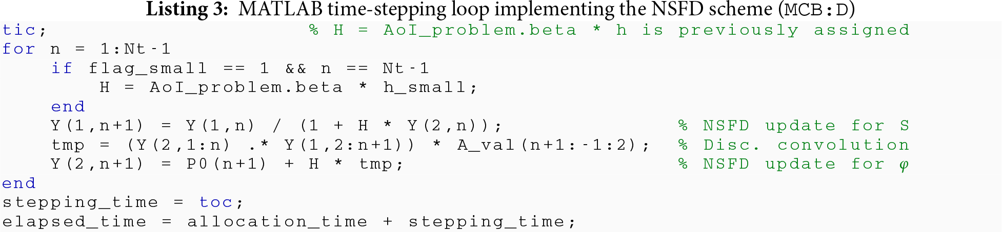
The core time-stepping blocks implementing the NSFD update are shown in Listings 3 and 4. Both versions rely on vectorized operations and compute the discrete convolution through optimized matrix-vector products, thus avoiding explicit summation loops. A minor implementation detail concerns the case in which the final time T is not an integer multiple of the prescribed step-size h. In this situation, the boolean flag flag_small activates a final reduced step of size h_small. This technical adjustment does not alter the convergence order of the NSFD method and does not affect its structure-preserving properties.

In addition to the core solver, the implementation relies on two auxiliary functions that handle input parsing and validation. Their purpose is to define default parameter values, complete missing entries and ensure the consistency of the problem definition before the time-stepping begins. The first auxiliary function, denoted parse_input in MATLAB (MCB:F) and_parse_input in Python (PCB:F), collects the user-provided arguments and fills any missing values with predefined defaults. In MATLAB, the defaults are

and in Python the corresponding dictionary is

If the field phi0 is not provided, it is automatically defined as φ0(t)=(N−S0)A(t). The function also emits warnings for missing fields when the verbosity flag is active.

The second auxiliary function, check_input in MATLAB (MCB:G) and _check_input in Python (PCB:G), verifies all input fields in accordance with the properties summarized in Table 1. Scalar parameters such as S0, N, T, h and β0 are required to be positive, finite and of the correct type. In MATLAB this is enforced via validateattributes, for example

while in Python an analogous test is

Furthermore, vector inputs corresponding to the kernel A(t) and the function φ0(t) are checked for non-negativity and elementwise consistency, i.e., φ0(tn)≤(N−S0)A(tn) for each n. In MATLAB, this is implemented via vectorized comparisons

and in Python using NumPy operations

Any violation of essential constraints triggers an error that immediately stops execution, whereas minor inconsistencies generate warnings if the verbosity flag is active. This layered validation ensures that the solver operates on a fully defined and consistent problem before entering the time-stepping phase.

4.2 The NSFD_behavioural Software

The NSFD scheme (9a)–(9c) for the behavioural model is developed in both MATLAB and Python within the function NSFD_behavioural. Specifically, our codes implement the non-standard discretization of (2), expressed in terms of the standardized quantities

sn≈S(tn)N,fn≈F(tn)N,mn≈M(tn)N,(17)

with normalization factor N:=λ/μ, corresponding to the total population size.

The NSFD_behavioural solver supports both structured inputs and explicit argument passing, with default values automatically assigned whenever optional parameters are omitted. The primary inputs are described below:

•   the final time T and the step-size h,

•   the initial susceptible population S0,

•   the total population size N and the natural death rate μ,

•   the infectivity function Aμ(t), the memory kernel K(t), the inhibition function β(M) and the message function g(F),

•   a boolean parameter compGamh for the automatic computation of the cutoff index (0 to disable it, 1 to enable it),

•   a verbosity binary flag that controls warning messages (0 to suppress them, 1 to enable them).

As main outputs, the epidemiologically most relevant quantities only are retained, sn and fn, leaving out the auxiliary memory variable mn. Accordingly, the solver returns the discrete time vector t and the solution matrix Y, whose n-th column stores the discrete approximations [sn,fn]T as defined in (17).

The corresponding approximations for the functions in the original model (2) may be retrieved by multiplying these normalized values by the constant N. Additionally, an optional performance object P can be returned upon request. This object contains numerical details about the computation and is implemented as a structured array in MATLAB and as a dictionary in Python, as shown in Listings 5 and 6, respectively.

The execution time (elapsed_time) is recorded using native timing utilities in the two environments, namely the tic/toc pair in MATLAB and the time.time() function in Python. The amount of memory required by the algorithm (memory_bytes) is evaluated by relying on built-in inspection tools, specifically the whos command in MATLAB and the .nbytes property in Python. The total number of floating-point operations (flops_number) is estimated by explicitly counting the arithmetic operations performed at each time step. The update of Sn+1 involves a fixed number of scalar operations, and the evaluation of the history-dependent terms requires the computation of two discrete convolutions. Overall, this results in approximately 6n+9 floating-point operations per time step. Summing over all time levels yields a total computational cost that scales quadratically with the number of time steps, leading to an overall complexity of 𝒪(Nt2). The metric Kern_number represents how many times the kernel functions Aμ(t) and K(t) are evaluated. In particular, the number of evaluations of Aμ(t) matches the number of time nodes, whereas the number Keval of memory kernel evaluations depends on the normalization cutoff strategy (see Section 3.2.1).

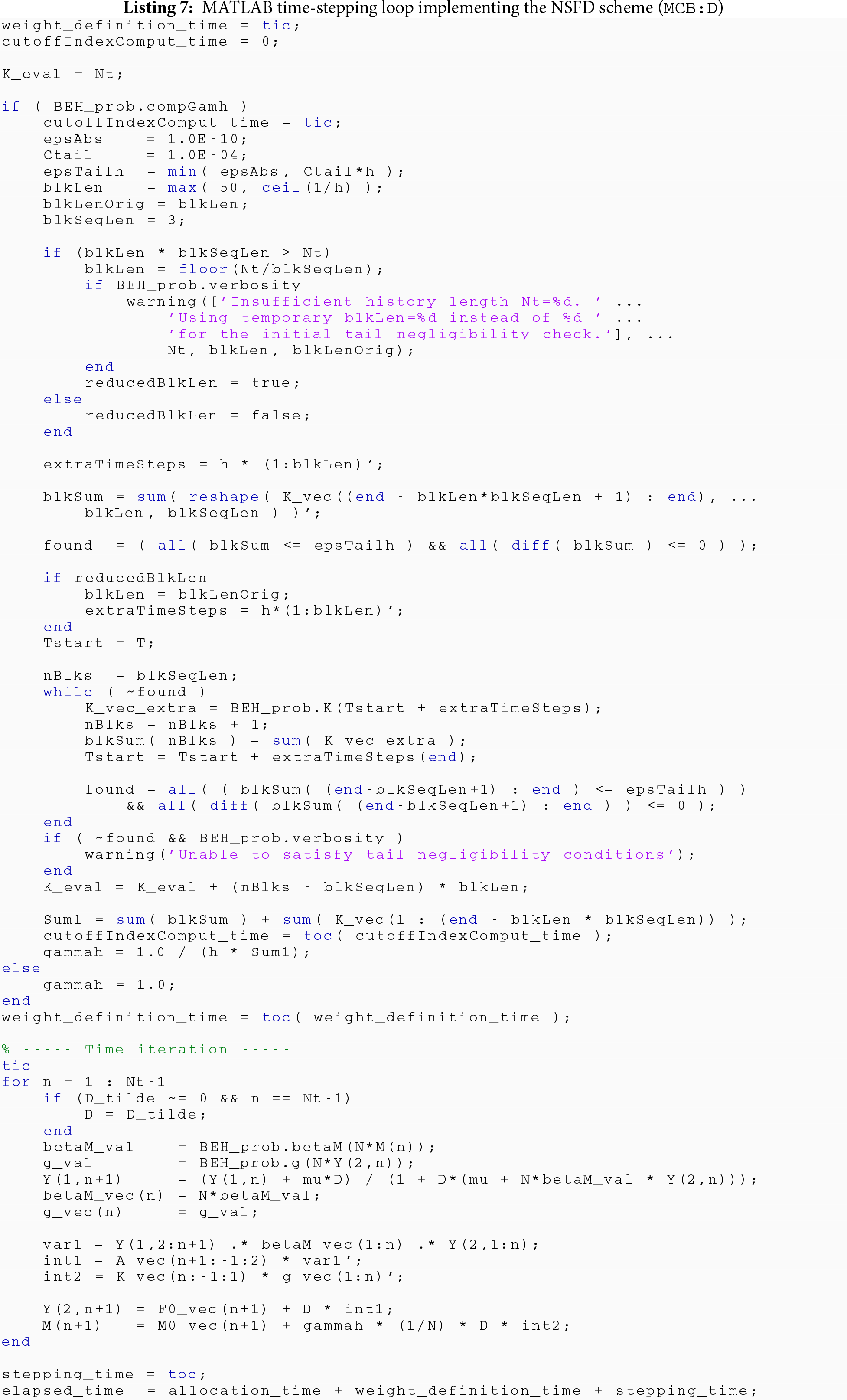
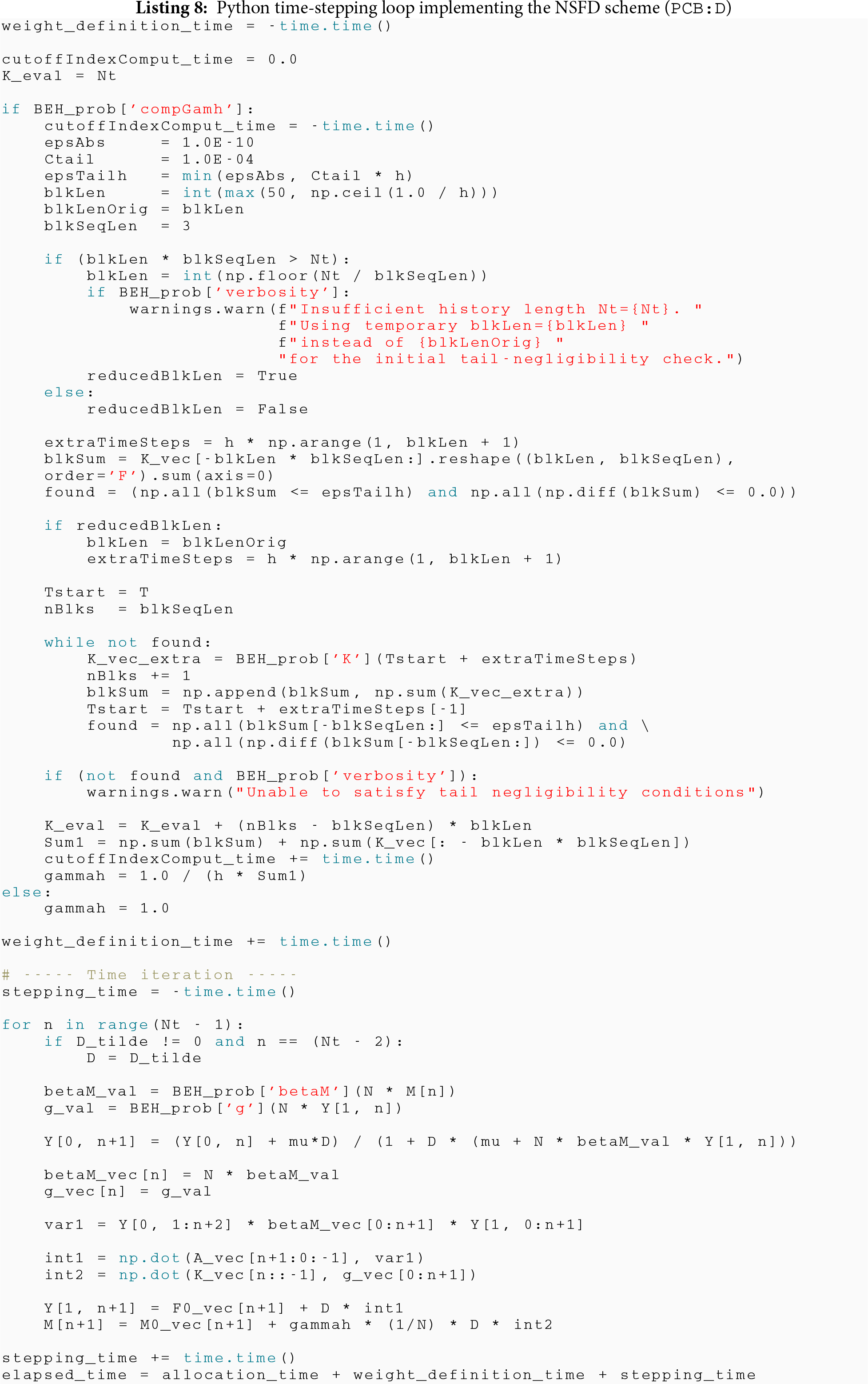
The core time-stepping routines for the present method (see Listings 7 and 8) adhere to the same implementation principles outlined in the previous section. A minor yet relevant difference is the preliminary computation of the non-standard weight γ(h), which appears in Eq. (9c) and is computed prior to advancing the solution in time. Its analytical expression is provided in (11). In the numerical implementation, the infinite series defining γ(h) is truncated by considering a sufficiently large number of terms as illustrated in Section 3.2.1. The subsequent updates are then performed using vectorized operations, with the history-dependent terms evaluated through optimized matrix–vector products, thus avoiding explicit summation loops. As before, when the prescribed step-size h does not exactly match the final time T, a reduced final step of length h_last is exploited. This technical detail preserves both the convergence order and the structure-preserving features of the underlying NSFD scheme.

Similarly to the NSFD_AoI function, the solver NSFD_behavioural is complemented by auxiliary routines devoted to input parsing and validation. These auxiliary modules assign default values, complete missing parameters and verify the consistency of the problem setup before the time-stepping phase. Since their functionality mirrors that already described in Section 4.1, only the differences in the prescribed default values are reported here. The input-handling function is denoted by parse_input in MATLAB (MCB:F) and the default parameters are set as follows:

The corresponding function in Python is denoted as _parse_input (PCB:F), and the default parameters are

If any of the core functions are not provided, they are automatically initialized with the following default definitions

g(x)=x,A(t)=R0(μ+ν)2te−(μ+ν)t,K(t)=ae−at,β(x)=(1+αx)−1,

with R0=20, ν=1/7, a=1/30, and α=8⋅103. When the verbosity flag is enabled, the routine also issues warnings for any missing optional fields. Furthermore, an auxiliary routine checks the validity of all input fields. In MATLAB, this is performed by the local function check_input (MCB:G), and in Python by _check_input (PCB:G). The checks ensure that scalar parameters such as S0, N, T, h and μ are positive and finite, using the same mechanisms described earlier (e.g., validateattributes in MATLAB).

4.3 Graphical User Interface

The interdisciplinary nature of epidemic modelling often requires numerical tools to be used by researchers and professionals whose expertise lies in epidemiology, public health or policy planning rather than in numerical analysis and scientific programming. To address this need, EPITIME includes a MATLAB Graphical User Interface (GUI) that provides direct access to the AoI simulation tool without requiring users to modify or run the underlying code. Practical instructions for launching and operating the interface are reported in Appendix B.3.

Through the GUI, users can specify the epidemiological parameters and the model functions A(t) and φ0(t), inspect their profiles and run the structure-preserving NSFD scheme. The interface displays the resulting susceptible population S(t) and mean infectivity φ(t), while also reporting consistency checks, warnings and performance information. It therefore provides an interactive environment in which different assumptions on infection-age-dependent infectivity and initial epidemic history can be examined without direct interaction with the numerical implementation.

Fig. 1 shows the interface after a simulation with the default functions

A(t)=e−3t,φ0(t)=(N−S0)A(t),

and parameters N=1000, S0=990, T=10, h=0.1 and β0=0.0025. The upper plots allow the prescribed infectivity profile and initial history to be checked before interpreting the numerical solution, whereas the lower plots display the corresponding evolution of susceptibility and mean infectivity.

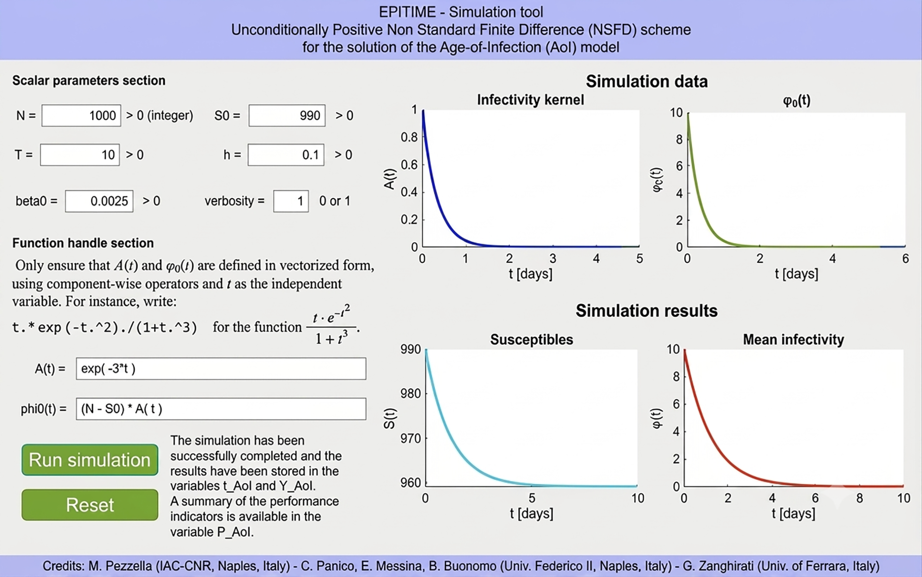
Figure 1: The AoI simulation GUI after a successful run with the default model functions A(t)=e−3t and φ0(t)=(N−S0)A(t), and parameters N=1000, S0=990, T=10, h=0.1 and β0=0.0025.

Two representative examples illustrate how the GUI can support numerical exploration. In the first test, the functions

A(t)=te−t,φ0(t)=104te−t1+t2

are considered together with N=106, S0=9⋅104, T=10, h=10−2 and β0=10−6. As shown in Fig. 2, the interface makes it possible to inspect the non-monotone infectivity profile and the prescribed initial history alongside the epidemic trajectories generated by them. This example also demonstrates that model functions and parameter scales substantially different from the default configuration can be investigated directly through the interface.

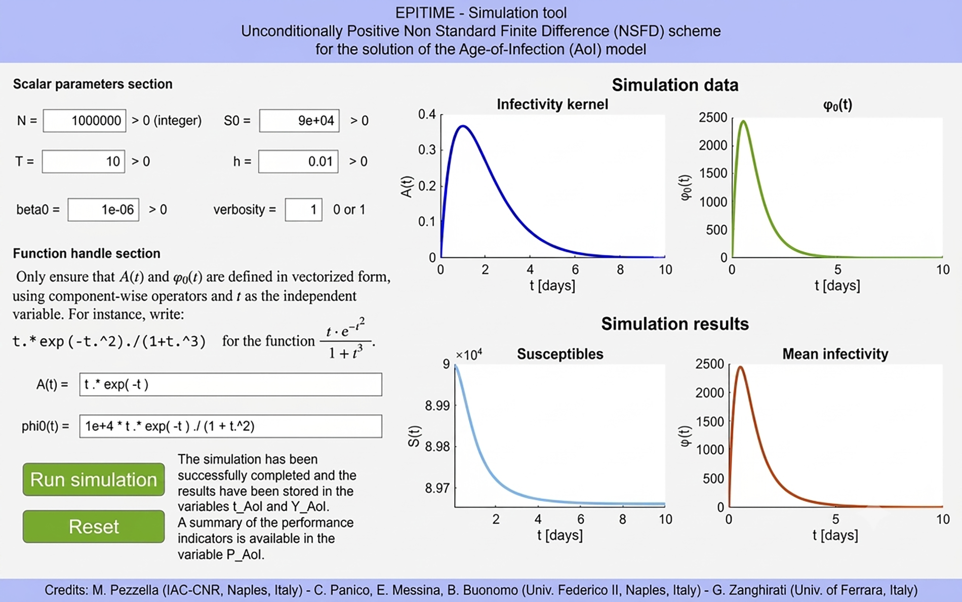
Figure 2: The AoI simulation GUI for N=106, S0=9⋅104, T=10, h=10−2 and β0=10−6, with A(t)=te−t and φ0(t)=104te−t/(1+t2).

The second test reproduces the experiment defined in (20) and discussed in Section 5.2. In this case, the GUI connects the analytical results with their numerical counterpart by allowing the predicted asymptotic behaviour to be examined directly from the computed profiles. Fig. 3 shows the resulting simulation. More generally, this type of experiment enables users to vary the model data and assess how infection-age profiles and epidemiological parameters affect transient and long-time dynamics.

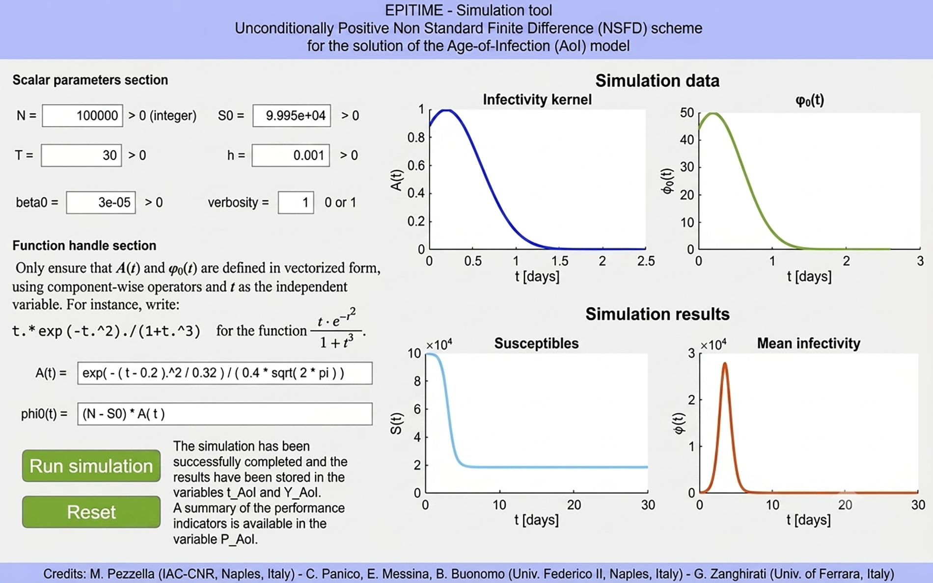
Figure 3: The AoI simulation GUI for the test case defined in (20) and discussed in Section 5.2.

A Python interface with equivalent functionality is also provided in the EPITIME repository as an interactive Jupyter notebook (AoI_Simulation_Tool.ipynb).

4.4 Theoretical Assumptions and Software Validation

The analytical properties stated in Sections 2 and 3 rely on the assumptions listed in Tables 1 and 2. In particular, the infectivity and memory kernels are assumed to be non-negative and integrable on R0+. Additional regularity assumptions, such as A∈C1([0,T]) for the AoI model and Aμ,K∈C1([0,T]) for the behavioural model, are required only for the first-order convergence results. Further assumptions on Aμ′ and K′ are used in the analysis of the asymptotic properties.

In the software implementation, only those assumptions that can be checked numerically are enforced. Specifically, the sampled values of the user-defined kernels on the computational grid are required to be finite and non-negative. For the behavioural model, the discrete memory kernel is normalized through the factor γ(h), or through its truncated counterpart γLK(h) when tail truncation is used. Smoothness and integrability over the whole semi-infinite interval remain mathematical assumptions under which the theoretical guarantees of the method hold true.

If a user provides kernels that violate the numerical checks, the solver returns an error or a warning, depending on the severity of the violation. When the analytical assumptions are not satisfied, the code may still produce a numerical trajectory, but the structure-preserving and convergence results proved in the paper are no longer guaranteed.

5  Numerical Experiments and Case Studies

This section presents numerical experiments designed to illustrate the accuracy, structure-preserving properties, and practical applicability of the proposed schemes.

5.1 Performance Analysis

The evaluation of the history-dependent convolution terms in (1) and (2) requires the accumulation of contributions from all previously computed time levels. Consequently, as discussed in Section 4, the computational cost of the proposed software framework is expected to scale quadratically with respect to the number Nt of time steps. To assess this prediction experimentally, we perform a dedicated computational complexity study for both the MATLAB and Python implementations of the NSFD_AoI and NSFD_behavioural solvers.

The analysis is carried out on the fixed time interval [0,T], with T=100, while progressively increasing the number of time steps from 10 to 104 in increments of 10. For each discretization level, the time step is defined as h=T/Nt, and the solver is executed using its default model parameters. For the behavioural solver, the automatic computation of the discrete normalization factor is enabled. In this way, the reported measurements also account for the execution of the auxiliary routines devoted to input parsing and consistency verification, whose computational cost is expected to remain negligible with respect to the overall integration process.

Specifically, two performance indicators are considered. The first is the execution time. In MATLAB, this quantity is measured through the built-in timeitroutine, which automatically performs multiple evaluations of the target function and returns a statistically robust estimate of the execution cost. In Python, the execution time is measured through the standard timeit module by performing several batches of repeated solver evaluations and retaining the minimum average runtime. This procedure closely mirrors the philosophy of MATLAB’s timeit routine and reduces the influence of transient system disturbances. The second indicator is the memory requirement. For both implementations, this quantity is extracted from the optional performance structure P returned by the solver (cf. Listings 5 and 6).

Fig. 4 reports the NSFD_AoI runtime and memory requirements in semi-log scale together with the reference growth laws 𝒪(Nt) and 𝒪(Nt2). The observed behaviour closely follows the theoretical complexity predicted by the structure of the algorithms. In particular, the memory consumption exhibits an essentially linear growth with respect to Nt, reflecting the storage of the numerical solution history together with the precomputed kernel values. Conversely, the execution time displays a clear quadratic scaling, consistently with the repeated evaluation of the discrete convolution terms appearing in the renewal equations. For a more detailed tabulation of the results, the reader is referred to the scripts AoI_Performance_Benchmark.m and AoI_Performance_Benchmark.pyavailable in the EPITIME repository.

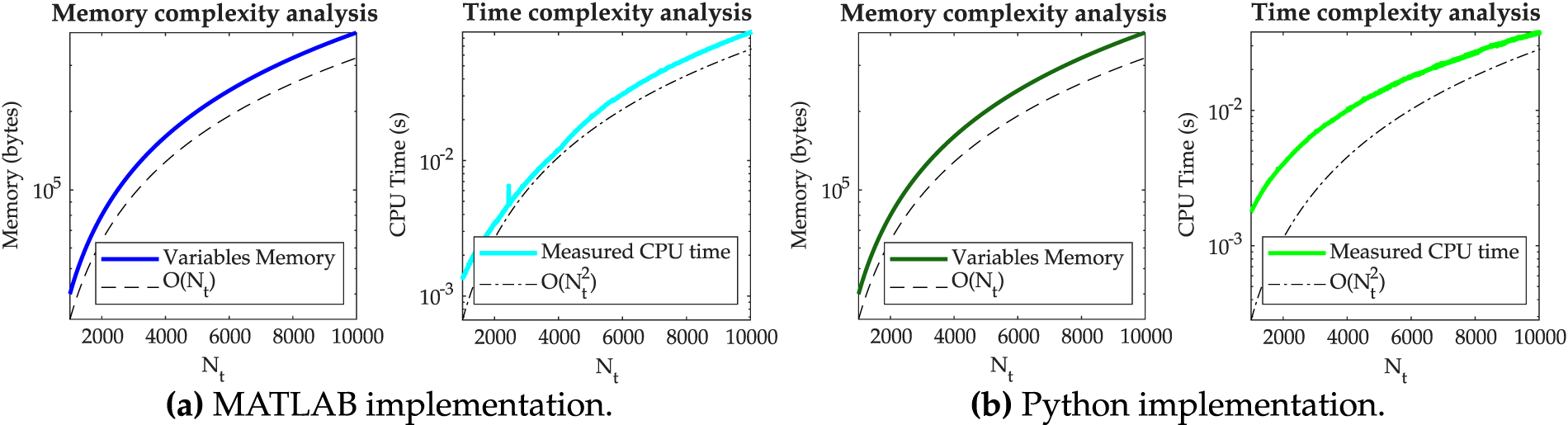
Figure 4: Experimental scalability analysis of the NSFD_AoI solver implemented in MATLAB (a) and Python (b). For both implementations, memory consumption (left panel within each subfigure) and execution time (right panel within each subfigure) are reported as functions of the number Nt of time steps.

Similar outcomes, reported in Fig. 5, are obtained for both the implementations of the NSFD_behavioural solver.

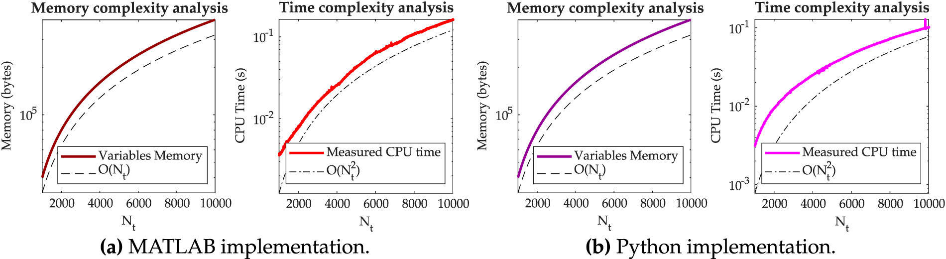
Figure 5: Experimental scalability analysis of the NSFD_behavioural solver implemented in MATLAB (a) and Python (b). For both implementations, memory consumption (left panel within each subfigure) and execution time (right panel within each subfigure) are reported as functions of the number Nt of time steps.

5.2 The Final Size and the Basic Reproduction Number

The first test case examines the asymptotic behaviour of the NSFD solution to (1), with particular emphasis on the convergence of the numerical final size towards its continuous counterpart. To begin with, recall that the final size of the epidemic, defined as S(∞)=limt→+∞S(t), satisfies the non-linear relation

log⁡(S0S(∞))=(1−S(∞)N)R0+β0∫0∞(φ0(τ)−(N−S0)A(τ))dτ,(18)

where

R0=β0N∫0∞A(τ)dτ(19)

is the basic reproduction number, that is the expected number of secondary cases generated by a single primary case in a fully susceptible population in the absence of interventions [1]. Furthermore, under suitable regularity assumptions (see, for instance, Section 3 in [46]) it follows that φ(t)→0 as t→∞.

At the discrete level, the numerical final size S∞(h) is guaranteed to exist by Theorem 2. In the present test, the asymptotic behaviour of the NSFD solution is approximated by the value S~∞(h) of the numerical simulation at a sufficiently large final time T. The corresponding numerical basic reproduction number is defined as

R0(h)=hβ0N∑n=0∞A(tn+1).

Note that, in addition to the assumptions listed in Table 1, if

A′∈L1(R0+)or∃𝒯∈R+ such that A(t) is monotonic for all t≥𝒯,

then R0(h) converges linearly to R0 as the step-size tends to zero (cf. Lemma 3.3 in [12] and p. 208 in [47]). Furthermore, it has been shown in [12] that R0(h) plays, for the discrete dynamics, a role analogous to that of R0 in the continuous model, and that a discrete counterpart of the classical final-size relation (18) holds true Theorem 4.4 in [12]. To illustrate these theoretical considerations, consider the problem defined by

N=105,S0=99950,β0=3⋅10−5,T=30,A(t)=10.42πexp⁡(−(t−0.2)22⋅0.42).(20)

Specifically, the scenario in which φ0(t) attains its upper bound in (6) for all t is addressed. As a result, the values S(∞)=1.8389⋅104 and R0=2.0744 follow from (18) and (19), respectively. The numerical solution computed by the NSFD integrator (7) with step-size h=10−3 is displayed in Fig. 6. The NSFD scheme (7) is applied for four progressively refined step-sizes h=10−i, with i=1,…,4, and the values of R0(h),S~∞(h), and φ∞(h) are computed for each discretization level. The simulation results, reported in Table 3, show that the numerical final size S~∞(h) converges linearly to S(∞) as the step-size decreases. As outlined in [48], the convergence of the asymptotic limit is a non-trivial property arising from the dynamical consistency of the method (see also Theorem 4.1 in [12]). Additionally, φ∞(h) attains values close to machine precision, confirming the expected extinction of the total infectivity.

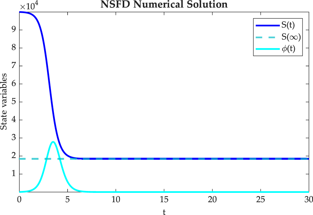
Figure 6: Time evolution of the susceptible population S(t) and total infectivity φ(t) for the AoI test case (20), computed with the NSFD scheme (7) and h=10−3. The horizontal line represents the continuous final susceptible population S(∞). The computed profiles illustrate the monotone decrease of S(t) and the decay of φ(t) towards zero.

To further illustrate the importance of structure-preserving discretizations, we repeat the previous experiment with β0=6⋅10−5, while keeping all the remaining parameters unchanged. The resulting problem is solved by both the NSFD scheme (7) and the second-order implicit Trapezoidal Direct Quadrature (TrapDQ) method

Sn+1=Sn−h2β0(Sn+1φn+1+Snφn),n=0,…,Nt−1,φn+1=φ0(tn+1)+h2β0(2A(tn+1)S0φ0+∑j=1nA(tn+1−j)Sjφj+2A(0)Sn+1φn+1).

Although more accurate for sufficiently small step-sizes, the TrapDQ method produces physically inadmissible solutions for h=0.25 (see Fig. 7). In particular, both S(t) and φ(t) become negative, and S(t) even exceeds the total population size N, despite the assumption of a closed population. In contrast, the NSFD approximation remains non-negative and satisfies the expected population bounds throughout the simulated interval. This experiment illustrates the unconditional structure-preserving behaviour of the NSFD scheme in a coarse-step regime.

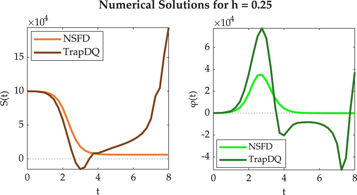
Figure 7: Comparison between the NSFD and TrapDQ solutions for the AoI test case (20), with β0=6⋅10−5 and h=0.25. The susceptible population S(t) is shown in the left panel and the total infectivity φ(t) in the right panel. The NSFD scheme preserves positivity and the population bounds, whereas the TrapDQ solution becomes negative and produces values of S(t) exceeding the total population size.

5.3 An Inverse Problem Framework for Inferring COVID-19 Infectivity Kernel

Despite the modeling potential of the integro-differential system (1), the identification of a contact rate β0 and an infectivity kernel A(t) that accurately reflect a real epidemic scenario remains a challenging task. Similar problems have been addressed in different settings, including the reconstruction of time-varying transmission rates [49], inverse formulations for integral epidemic models [50], and data-driven identification of distributed memory kernels [51]. This section proposes a case study to investigate the reliability of the EPITIME software as a tool to support the reconstruction of infectivity-kernel profiles in a real-world epidemic setting. To overcome this challenge, a functional optimization procedure is introduced, informed by empirical incidence and demographic data. In particular, the daily number of newly reported COVID-19 cases across Italy is considered, as reported by Il Sole 24 Ore [52], covering the period from February 24, 2020, to January 8, 2025 (T=1781 days), along with the total resident population N=58,934,177, according to the demographic data provided by Eurostat [53].

Focusing on the first equation of model (1), the normalized incidence and its NSFD approximation are defined as

𝒥(t)=κ𝒥β0S(t)φ(t),t∈[0,T],and𝒥n=κ𝒥β0Snφn,n=0,…,Nt,

where κ𝒥 is a normalization constant extracted from the data. Let 𝒥idata≈𝒥(τi), for i=0,…,Ndata, denote the empirical incidence at time τi, obtained from [52] and preprocessed to mitigate reporting noise and daily fluctuations, by applying a local regression smoothing procedure (MATLAB smoothdata, with loess option and smoothing factor 0.25), followed by normalization with respect to κ𝒥=maxi𝒥idata (see Fig. 8). These empirical values are compared with the simulated sequence {𝒥ni}i=0Ndata, where ni satisfies τi=nih.

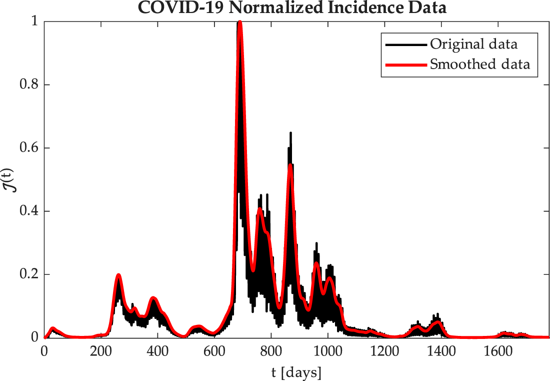
Figure 8: Normalized daily COVID-19 incidence in Italy (24 February 2020–8 January 2025), including raw data from [52] and the corresponding smoothed profile obtained via quadratic regression. Here, the normalization is performed with respect to the maximum value, yielding κ𝒥≈5.68⋅10−6.

To select a functional form for the kernel A(t), it is expanded in terms of shifted Bernstein basis polynomials (see, e.g., [54]). Given a positive ℳ∈N, representing the maximum polynomial degree, it is assumed that

A(t)=∑m=0ℳκmBmℳ(tT)=∑m=0ℳκm(ℳm)(tT)m(1−tT)ℳ−m,φ0(t)=(N−S0)A(t),t∈[0,T],

where the coefficients κm, m=0,…,ℳ, are unknown parameters to be determined. Owing to the non-negativity of the Bernstein basis, A(t) is guaranteed to remain non-negative if κm≥0 for all m. Consequently, we formulate a calibration problem for the parameter vector p=[β0,κ0,…,κℳ]T∈R+ℳ+2, aiming to minimize the discrepancy between observed and simulated incidence data. The optimal parameter set p∗ is defined as the solution to the constrained optimization problem

minp∈R+ℳ+2(wL2∑i=0Ndata(𝒥idata−𝒥ni(p))Ndata+12+wpeak(𝒥ipeakdata−𝒥nipeak(p))2+winitial(𝒥0data−𝒥n0(p))2minp∈R+M+2  +wyear∑i=0364(𝒥idata−𝒥ni(p))2365)  subject to R~0(p)=β0NTℳ+1∑m=0ℳκm∈[R0lower,R0upper],(21)

which yields the data-informed contact rate β0∗ and infectivity kernel A∗(t)=∑m=0ℳκm∗Bmℳ(t/T). The objective functional in (21) combines four terms, each emphasizing a distinct aspect of the epidemic dynamics.

•   a mean squared error over the entire dataset, measuring the global discrepancy between observed and simulated incidences;

•   a peak error term, enforcing accuracy at the time of maximum observed incidence;

•   an initial-time penalty, ensuring consistency at the onset of the epidemic;

•   a yearly error term, enforcing accurate reconstruction of early-stage dynamics over the first 365 days.

The weights wL2, wpeak, winitial and wyear are determined according to a reciprocal-optimum strategy. Each weight is set as the reciprocal of the minimum value attained by the corresponding objective component when optimized independently (all other weights set to zero), ensuring balanced contributions within the overall functional. The additional constraint enforces positivity of the coefficients and restricts the truncated basic reproduction number

R~0=β0N∫0TA(t) dt=β0NTℳ+1∑m=0ℳκm,

to lie within a prescribed plausible range. These bounds, set to R0lower=5⋅10−10 and R0upper=5⋅101 in our case, may be refined if more precise estimates of the basic reproduction number become available.

The model calibration problem formulated in (21) is addressed in the MATLAB live script NSFD_AoI_LIVE. This implementation allows the user to select both the dimension of the Bernstein polynomial space (we take ℳ=500) and the optimization algorithm. Notably, the optimization procedure requires repeated evaluations of the direct temporal integration problem, making computational efficiency and long-term accuracy indispensable. These requirements are naturally met by the NSFD scheme (7), which provides stable and reliable results even over extended time horizons. For the present study, the optimization is performed using MATLAB’s fmincon routine with StepTolerance and OptimalityTolerance set to 10−14, ConstraintTolerance equal to 10−16 and automatic differentiation activated wherever possible to enhance efficiency. Furthermore, the solver NSFD_AoI is run with a time step h=0.25, which is smaller than the minimum interval between consecutive measurements. The results of the calibration are summarized in Fig. 9, where the simulated incidence is compared with the empirical data and the estimated infectivity kernel is depicted. The figure also reports the pointwise quadratic absolute error, whose mean value of 4.2% supports the robustness and accuracy of the implemented methodology in reconstructing the dynamics of a real epidemic.

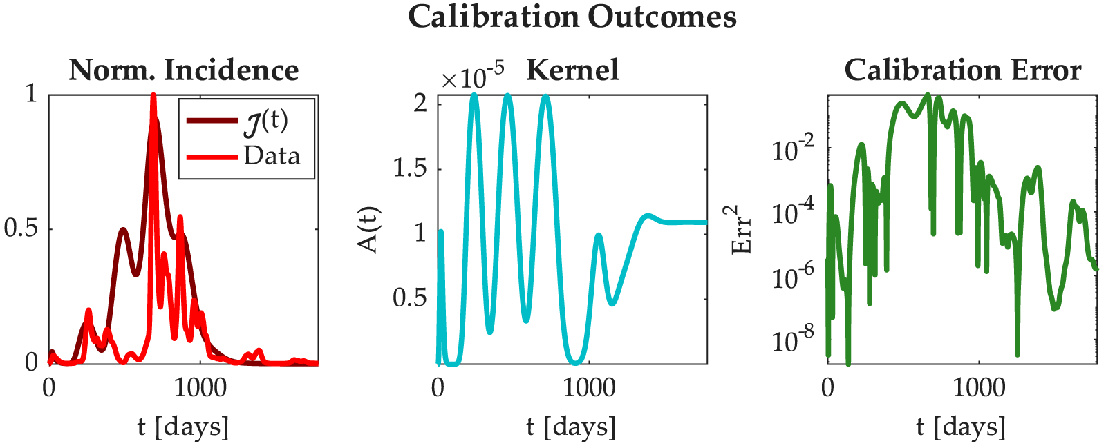
Figure 9: Comparison of the empirical COVID-19 normalized incidence in Italy with the simulated incidence (left panel), the corresponding estimated infectivity kernel (middle panel) and the pointwise quadratic error relative to the data (right panel). Here, the optimized contact rate is β0∗=2.18⋅10−5.

Remark 1: The present case study serves as a data-driven benchmark to assess the reliability of the EPITIME framework, rather than a standalone identifiability analysis. The underlying inverse problem is inherently ill-posed and presents several coupled methodological challenges. Specifically, the inverse map may lack full identifiability from incidence data, as distinct infectivity kernels can produce identical incidence trajectories. Regarding approximation, while the implicit smoothing of the Bernstein representation promotes stability, the procedure could benefit from explicit Tikhonov-type regularization (see, for instance, [55]). Furthermore, the characteristically slow convergence of Bernstein expansions requires high polynomial degrees to ensure sufficient representational capacity, leading to the heuristic selection of ℳ=500. Optimization is similarly challenging due to the non-convexity of the objective function, which does not preclude the existence of local minima. In this setting, MATLAB’s fmincon routine is used as a baseline gradient-based solver, although advanced strategies such as multistart and hybrid multigrid methods could enhance robustness with respect to the presence of local minima and the choice of the initial guesses. A systematic investigation of these approaches, complemented by a quantitative analysis of data uncertainty propagation, is deferred to future work.

5.4 Qualitative Properties of Solutions to the Integral Behavioural Epidemic Model

Before presenting the numerical experiments, the main qualitative properties of the behavioural integral epidemic model (2) and of its discrete counterpart (9a)–(9c) are briefly recalled. Under the assumptions stated in Section 3.2, the continuous model admits a positively invariant region, always possesses the disease-free equilibrium DFE, and admits a unique endemic equilibrium EE whenever R0>1. Moreover, the local stability of the equilibria depends on the specific choice of the infectivity function Aμ(t) and the memory kernel K(t). Specifically, suitable classes of kernels guarantee local asymptotic stability of the endemic state, whereas more structured memory effects may lead to instability and sustained oscillations [8]. The non-standard discretization (9a)–(9c) is designed so as to preserve these structural features: in particular, it maintains positivity and boundedness for every h>0, always admits a disease-free equilibrium, and admits a unique endemic equilibrium whenever the discrete threshold condition R0(h)>1 is satisfied, with R0(h) providing a first-order approximation of R0. In addition, the discrete characteristic equation is consistent with the continuous one as h→0, and the stability conditions derived for the numerical equilibria converge to the corresponding continuous conditions (see the results in [44] for a detailed analysis). The simulations reported below are intended to illustrate precisely this qualitative coherence between the continuous behavioural model and its NSFD approximation.

In this section, we illustrate two numerical examples based on the non-standard discretization (9a)–(9c) of model (2). In both experiments, the NSFD scheme is applied with h=10−1 and with the truncated-renormalized option for the discrete memory kernel, as described in Section 3.2.1. For all simulations:

g(F(t))=F(t),β(M(t))=11+αM(t).

The infectivity function Aμ(t) and the memory kernel K(t) are specified according to the particular scenario under consideration. The first experiment illustrates convergence toward the endemic equilibrium in a regime where stability is theoretically expected, whereas the second one highlights the onset of oscillatory behaviour induced by a more structured memory kernel.

For the first numerical experiment, the following values are considered:

T=1000,N=5⋅107,μ=175⋅365days−1,S0=0.99Se,α=8⋅103,(22)

where Se denotes the first coordinate of the endemic equilibrium. Furthermore, it is assumed that the infectivity function exhibits a unimodal profile and is given by

A(t)=β0te−νt,(23)

with Aμ(t)=e−μtA(t),ν=1/7 days−1. In this test R0=20 and the parameter β0 is determined so as to satisfy the condition for the basic reproduction number reported in Table 2, that is β0=(R0/N)(μ+ν)2.

Fig. 10 shows the time evolution of the driving factor of the FoI, F(t), normalized with respect to its endemic equilibrium value Fe. The results are obtained using the parameters in (22), the infectivity function defined in (23), and the memory kernel

K(t)=ae−at,(24)

with a=1/30 days−1. As shown in Fig. 10, the ratio F(t)/Fe converges asymptotically to one, indicating that the solution approaches the endemic equilibrium over time. This numerical behaviour is consistent with the theoretical findings in [8].

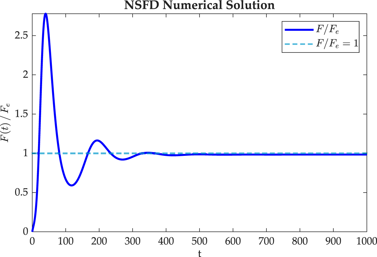
Figure 10: Normalized driving factor of the force of infection, F(t)/Fe, for the behavioural model with parameters (22), the unimodal infectivity function in (23), and the exponential memory kernel in (24). The solution is computed with the NSFD scheme (9a)–(9c) and h=10−1. The convergence of F(t)/Fe to one shows that the solution approaches the endemic equilibrium.

As a second numerical experiment, the trapezoidal infectivity function given by

A(τ)={p0τ−τa(τb−τa),τa<τ<τb,p0,τb<τ<τc,p0τd−τ(τd−τc),τc<τ<τd,0,otherwise,(25)

is considered instead, where Aμ(t)=e−μtA(t). Here, it is (τa,τb,τc,τd)=(4,7,11,14), where the parameter p0 represents the weight of contacts between infected and susceptible individuals. Additional details on the infectivity function (25) can be found in [56]. The value R0=3.3 is fixed and the parameter p0 is determined so as to satisfy the condition defining the basic reproduction number reported in Table 2. For this experiment, we adopt a different memory kernel, namely

K(t)=a2te−at,(26)

with a=1/30 days−1, and the parameters are chosen as

T=3000,N=5⋅107,μ=175⋅365d−1,S0=0.7N,α=5⋅104.(27)

The corresponding results are displayed in Fig. 11. As discussed in more detail in [8], in this case no convergence to the endemic equilibrium is observed. Instead, self-sustained oscillations arise, suggesting that the endemic equilibrium is numerically unstable.

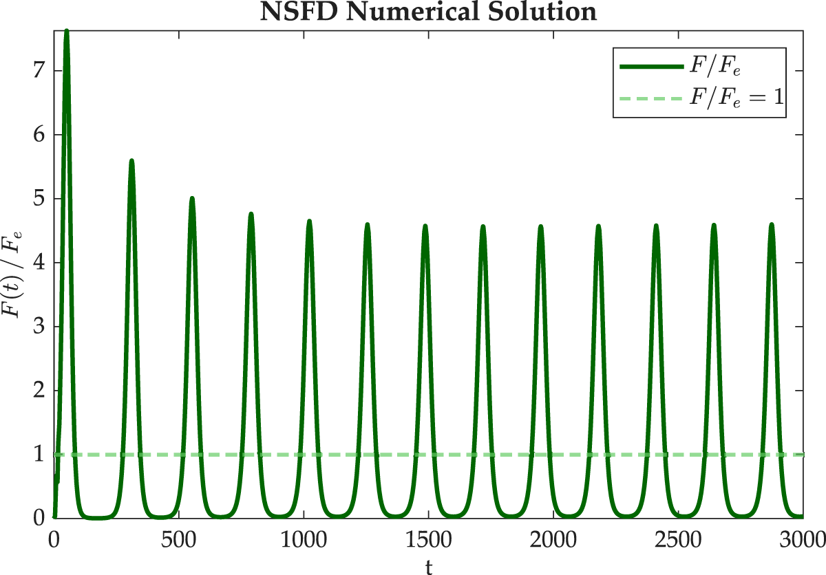
Figure 11: Normalized driving factor of the force of infection, F(t)/Fe, for the behavioural model with parameters (27), the trapezoidal infectivity function in (25), and the Erlang-type memory kernel in (26). The solution is computed with the NSFD scheme (9a)–(9c) and h=10−1. The combined effect of the trapezoidal infectivity distribution and the strong Erlang memory kernel gives rise to oscillations around F(t)/Fe=1 that appear to persist over time.

5.5 Estimation of the Epidemic Peak

A further computational task supported by EPITIME is the estimation of epidemic peaks and peak times. For classical compartmental models, and in particular for the autonomous SIR model, peak-time formulae and approximations have been investigated in several works [57–60]. Related peak-date estimates have also been obtained for generalized SEIR and infection-age structured models [61]. Recent renewal-equation analyses have also investigated final-size and peak-size relations for infection-age models incorporating latency and behaviour-dependent transmission. Analytical information on peak quantities can be obtained for some reduced model structures [62]. For general renewal and age of infection models with arbitrary infectivity kernels, closed-form peak-time formulae are generally unavailable, and peak quantities must be estimated from the numerical solution. For the AoI model (1), we define the epidemic peak and the corresponding peak time in terms of the force of infection as

Ep=β0max0≤t≤Tφ(t),tp=minarg⁡max0≤t≤Tφ(t).(28)

The minimum selects the first global peak when the maximum is attained at more than one time. At the discrete level, EPITIME computes

Ep(h)=β0maxn=0,…,Ntφn≈Ep,tp(h)=minarg⁡maxn=0,…,Ntφn≈tp.(29)

To validate this peak-detection procedure in a benchmark case where a SIR reference is available, the exponential infectivity kernel

A(t)=e−γt.

is considered. With this choice, the AoI formulation recovers the classical autonomous SIR dynamics. The reference peak times tp∗ are obtained from the corresponding SIR peak-time characterization, using parameter configurations taken from the SIR peak-time literature [60]. The numerical results reported in Table 4, obtained with h=10−3, show that EPITIME accurately captures the epidemic peak. Fig. 12 further shows that the relative error in the peak-time approximation decreases linearly with the time step, consistently with the first-order accuracy of the underlying NSFD scheme.

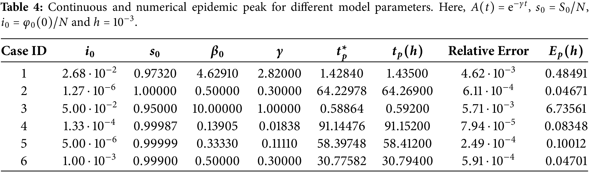
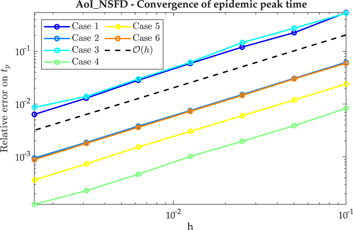
Figure 12: Convergence of the epidemic peak time approximation. The relative error exhibits a linear decay with respect to h for all considered parameter sets.

Regarding the behavioural model, in the context of epidemic peak estimation, we investigated both the driving factor of the FoI, F(t), and the incidence, inc(t)=β(M(t))S(t)F(t). Specifically, the incidence at each time step tn is numerically computed using the following expression, which relies exclusively on the values of the susceptible population:

incn=β(Mn)Sn+1Fn=N(sn−sn+1h+μ(1−sn+1)).

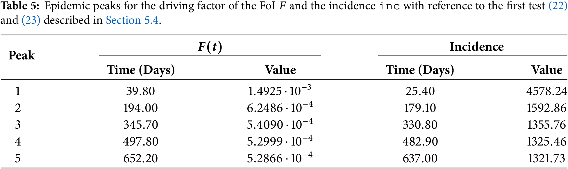
The corresponding numerical peak time is obtained as the time point associated with the maximum value of the selected observable. As illustrated in Fig. 13 and Table 5, when several local maxima occur, as may happen in the presence of behavioural feedback and memory, both local and global peak times can be reported.

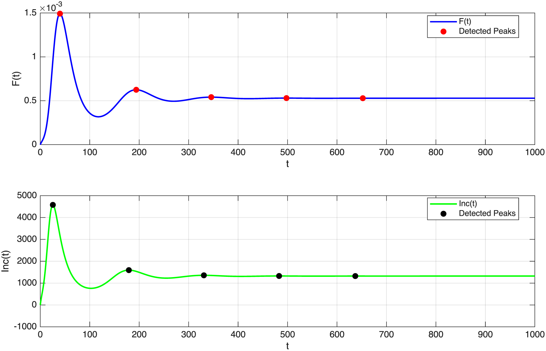
Figure 13: Epidemic peaks for the driving factor of the FoI F and the incidence inc with reference to the first test (22) and (23) described in Section 5.4.

6  Conclusions and Future Directions

A computational framework, EPITIME, has been developed for the simulation of two classes of renewal-type epidemic models: an age of infection model and an information-dependent behavioural model. The framework combines structure-preserving NSFD discretizations with modular implementations in MATLAB and Python. The solvers are complemented by input-validation routines, performance indicators, reproducibility tools and graphical interfaces. The numerical experiments have illustrated the use of the framework for the study of final-size behaviour, the reconstruction of an infectivity kernel from incidence data, the analysis of behavioural dynamics under different memory kernels, and the detection of epidemic peaks.

A main strength of EPITIME is the close connection between the analytical properties of the models and their numerical implementation. The schemes preserve model-specific properties such as positivity, monotonicity, boundedness, invariant regions, extinction of infectivity and equilibrium or threshold structure. This makes the framework particularly suitable for long-time simulations, for which standard discretizations may produce non-physical solutions. At the same time, the modular organization of the software allows the kernels and behavioural response functions to be changed without modifying the main solver structure.

The present release is intentionally focused on the two deterministic models considered in this work. This choice makes it possible to provide clear mathematical guarantees, but it also defines a natural path for future development. The framework is planned to be extended to a more general renewal formulation, which includes the age of infection model as a special case. Further extensions will address heterogeneous populations, the distinction between symptomatic and asymptomatic infections, and viral shedding effects. Vaccination dynamics also represent an important direction. In the AoI setting, vaccination could be introduced through additional vaccinated classes, allowing vaccine-induced changes in susceptibility, breakthrough infections and waning immunity to be represented within the renewal formulation. Vaccination-induced changes in infectivity could also be accounted for by suitable infectivity kernels. In the behavioural model, vaccine uptake could additionally be coupled with information-dependent responses and memory effects, extending ODE-based formulations with vaccination choices driven by information and perceived risk.

Further work will also concern the numerical methods. The schemes implemented in the current release are first-order accurate and favour robustness and structure preservation. Fine temporal grids may nevertheless be required when high accuracy is needed for rapidly varying solutions, peak times or peak sizes. Higher-order structure-preserving discretizations and more accurate procedures for the estimation of epidemic peaks will therefore be investigated. Their construction will have to retain the unconditional qualitative properties that characterize the present methods.

The direct vectorized evaluation of the history terms provides a transparent implementation that closely follows the discrete equations, but its computational cost is quadratic in the number of time steps. This may become restrictive for very long simulations or inverse problems involving repeated solver evaluations. Future versions are intended to include suitable acceleration strategies. For exponential and Erlang kernels, auxiliary recursions or linear-chain representations may reduce the computational cost to linear complexity. For more general kernels, possible approaches include FFT-based and other fast convolution techniques, and sum of exponentials approximations. A central part of this development will be the control of the additional approximation error and the verification that positivity, kernel normalization and equilibrium properties are not lost.

Finally, the theoretical guarantees of the solvers depend on assumptions on the user-defined kernels and behavioural functions, such as non-negativity, integrability and sufficient regularity. These conditions cannot all be verified automatically, and future releases will include more extensive diagnostic checks and clearer guidance on admissible inputs. The inverse reconstruction presented in this work should also be viewed as a computational benchmark rather than as a complete epidemiological inference procedure. Further investigations will address identifiability, regularization, data preprocessing, measurement noise and uncertainty propagation, together with validation on additional datasets. The graphical interfaces will be developed in parallel by adding context-sensitive help and concise instructions, with the aim of making the framework easier to use while preserving a clear connection with its mathematical background.

Acknowledgement: This work has been performed under the auspices of the Italian National Group for Scientific Computing (GNCS) and the Italian National Group for Mathematical Physics (GNFM) of the National Institute for Advanced Mathematics (INdAM).

Funding Statement: The authors received no specific funding for this study.

Author Contributions: The authors confirm contribution to the paper as follows: Conceptualization, Bruno Buonomo and Eleonora Messina; methodology, Eleonora Messina, Mario Pezzella and Gaetano Zanghirati; software, Claudia Panico, Mario Pezzella and Gaetano Zanghirati; validation, Bruno Buonomo, Eleonora Messina, Claudia Panico, Mario Pezzella and Gaetano Zanghirati; formal analysis, Claudia Panico, Mario Pezzella and Gaetano Zanghirati; investigation, Eleonora Messina, Claudia Panico, Mario Pezzella and Gaetano Zanghirati; data curation, Mario Pezzella; writing—original draft preparation, Claudia Panico, Mario Pezzella and Gaetano Zanghirati; writing—review and editing, Bruno Buonomo, Eleonora Messina, Mario Pezzella and Gaetano Zanghirati; visualization, Claudia Panico, Mario Pezzella and Gaetano Zanghirati; supervision, Bruno Buonomo, Eleonora Messina, and Gaetano Zanghirati. All authors reviewed and approved the final version of the manuscript.

Availability of Data and Materials: The EPITIME software described in this work is publicly available at https://github.com/ghitan/EPITIME (accessible since May 6, 2026). The numerical results presented in this paper were obtained with version 1.0. The software is distributed under the GNU General Public License v3.0 (GPL-3.0). The data that support the findings of this study are openly available at [52] and [53].

Ethics Approval: Not applicable.

Conflicts of Interest: The authors declare no conflicts of interest.

Abbreviations

The following abbreviations are used in this manuscript:

Appendix A Unified Notation Guide

Table A1 provides a unified notation guide for the continuous variables, discrete quantities, and implementation-level variables used throughout the manuscript. The assumptions associated with each model are reported separately in Tables 1 and 2.

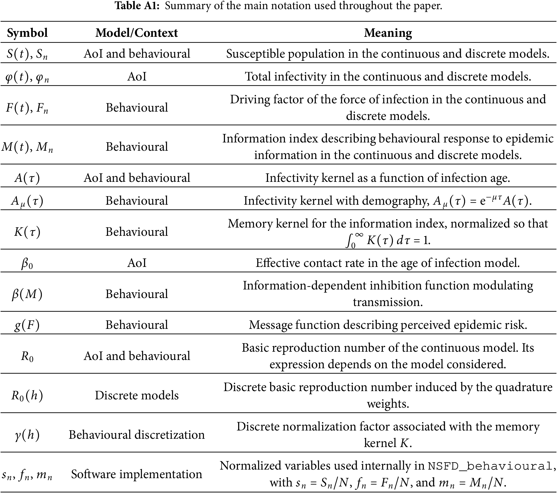
Appendix B Software Validation and Reproducibility

All numerical experiments presented in this paper can be reproduced using the publicly available implementations provided in the EPITIME repository. Relevant information concerning the software environment, hardware platform, code version and dependencies of the solvers codes is reported in Table A2. We point out that the MATLAB Optimization Toolbox is used exclusively for the kernel calibration in Section 5.3. It is not part of the EPITIME framework and is required only for this specific application.

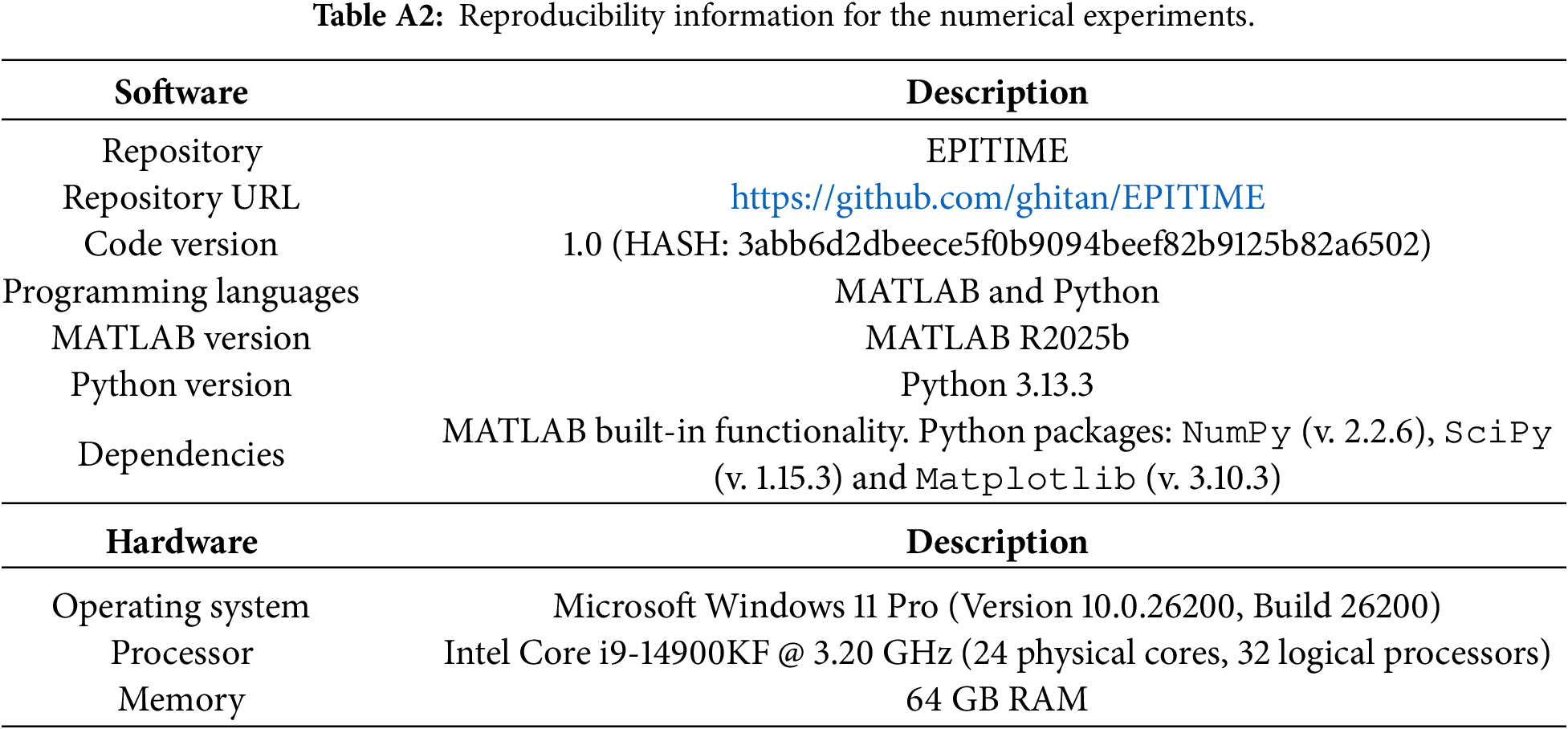
Appendix B.1 Organization of the Github Repository

This appendix lists the source files in the EPITIME GitHub repository associated with the numerical experiments and examples presented throughout the manuscript.

•   Section 4.1—Codes: NSFD_AoI.m and NSFD_AoI.py

•   Section 4.2—Codes: NSFD_behavioural.m and NSFD_behavioural.py

•   Section 5.1—Codes: AoI_Performance_Benchmark.m, AoI_Performance_Benchmark.py, behavioural_Performance_Benchmark.m and behavioural_Performance_Benchmark.py

•   Section 5.2—Codes: AoI_Final_Size.m and AoI_Final_Size.py

•   Section 5.3—Code: NSFD_AoI_LIVE.mlx (Part 3.4)

•   Section 5.4—Codes: Behavioural_unimodal_IF.m, Behavioural_trapezoidal_IF.m, Behavioural_unimodal_IF.py and Behavioural_trapezoidal_IF.py

•   Section 5.5—Codes: AoI_Peak_Estimation.m, AoI_Peak_Estimation.py, Behavioural_Peaks_Estimation.m and Behavioural_Peaks_Estimation.py

Appendix B.2 Cross-implementation Verification

In what follows, we perform a cross-implementation verification of the EPITIME computational framework. To this end, the benchmark problems presented in Section 5 are independently reproduced using both the MATLAB and Python implementations, and the quantities of interest generated by the two software versions are systematically compared.

Concerning the AoI model, the test problem defined by (1)–(20) is chosen. For every simulation and for both implementations, the discrete solution sequences {Snℓ(h)}n=0Nt and {φnℓ(h)}n=0Nt are stored. Here, the superscript ℓ∈{M,P} denotes the solution computed by the MATLAB and Python codes, respectively. In particular, the numerical discrepancies are quantified through the relative L2-errors defined as follows

ℰ2S(h)=∑n=0Nt|SnM(h)−SnP(h)|2∑n=0Nt|SnM(h)|2,ℰ2φ(h)=∑n=0Nt|φnM(h)−φnP(h)|2∑n=0Nt|φnM(h)|2,

and the asymptotic behaviour mismatches are addressed with the following pointwise final-time differences

ℰ∞S(h)=|S~∞M(h)−S~∞P(h)|S~∞M(h),ℰ∞φ(h)=|φ∞M(h)−φ∞P(h)|φ∞M(h).

The results of the comparison, reported in Table A3, show errors at the level of machine precision and confirm the consistency of the two independent implementations. Analogous outcomes are obtained by comparing the two implementations of the NSFD_behavioural solver.

Appendix B.3 Practical Use of the Graphical Interface

The MATLAB GUI currently supports the AoI model only. It is distributed as the file EPITIME_SimulationTool.mlapp, together with the associated software resources. It can be launched from the Apps panel in the MATLAB main window or opened directly from the folder containing the application file.

The interface is organized into two main panels. The left panel contains the model inputs and simulation controls, while the right panel displays the input functions and numerical results. The upper part of the left panel contains the parameters required by the NSFD_AoI function, as described in Section 4.1. Each field is initialized with its default value and accepts only inputs satisfying the prescribed type and range constraints.

The functions A(t) and φ0(t) are entered as MATLAB expressions in the corresponding text fields. The independent variable must be denoted by t, and the expressions must support vector inputs. For simple functions, vectorized one-line expressions can be entered directly. More complex functions may instead be implemented in external MATLAB files, with the corresponding function calls entered in the GUI. In both cases, the expressions are automatically converted into function handles and passed to the main simulation routine.

The Run simulation button starts the computation, whereas Reset restores all fields to their default values. A message area reports validation errors, warnings and information returned by the NSFD_AoI routine.

The upper part of the output panel displays the profiles of A(t) and φ0(t). These plots are updated when the corresponding expressions are entered. After a successful simulation, the lower part displays the computed susceptibility S(t) and mean infectivity φ(t).

The complete numerical output is also exported automatically to the MATLAB workspace. The variables t_AoI, Y_AoI and P_AoI contain, respectively, the time grid, the numerical solution and the performance data. They can therefore be used for additional processing, plotting or comparison outside the GUI.

References

1. Brauer F, Castillo-Chavez C, Feng Z. Mathematical models in epidemiology. New York, NY, USA: Springer; 2019. doi:10.1007/978-1-4939-9828-9. [Google Scholar] [CrossRef]

2. Martcheva M. An introduction to mathematical epidemiology. In: Texts in applied mathematics. New York, NY, USA: Springer; vol. 61, 2015. doi:10.1007/978-1-4899-7612-3. [Google Scholar] [CrossRef]

3. Kermack WO, McKendrick AG. A contribution to the mathematical theory of epidemics. Proc R Soc Lond Ser A Contain Pap A Math Phys Character. 1927;115(772):700–21. doi:10.1098/rspa.1927.0118. [Google Scholar] [CrossRef]

4. Breda D, Diekmann O, de Graaf WF, Pugliese A, Vermiglio R. On the formulation of epidemic models (an appraisal of Kermack and McKendrick). J Biol Dyn. 2012;6(sup2):103–17. doi:10.1080/17513758.2012.716454. [Google Scholar] [CrossRef]

5. Diekmann O, Inaba H, Thieme HR. Mathematical epidemiology of infectious diseases: an ongoing challenge. Jpn J Ind Appl Math. 2025;42(4):1563–90. doi:10.1007/s13160-025-00742-1. [Google Scholar] [CrossRef]

6. Manfredi P, d’Onofrio A, editors. Modeling the interplay between human behavior and the spread of infectious diseases. New York, NY, USA: Springer; 2013. doi:10.1007/978-1-4614-5474-8. [Google Scholar] [CrossRef]

7. Bai Z. Global dynamics of a SEIR model with information dependent vaccination and periodically varying transmission rate. Math Methods Appl Sci. 2014;38(11):2403–10. doi:10.1002/mma.3231. [Google Scholar] [CrossRef]

8. Buonomo B, Messina E, Panico C, Vecchio A. An integral renewal equation approach to behavioural epidemic models with information index. J Math Biol. 2024;90(1):8. doi:10.1007/s00285-024-02172-y. [Google Scholar] [CrossRef]

9. Buonomo B, Messina E, Panico C. Minimal epidemic models with information index: from compartmental to integral formulation. Boll Unione Mat Ital. 2025;18(4):1181–202. doi:10.1007/s40574-025-00473-8. [Google Scholar] [CrossRef]

10. d’Onofrio A, Manfredi P. Information–related changes in contact patterns may trigger oscillations in the endemic prevalence of infectious diseases. J Theor Biol. 2009;256(3):473–8. doi:10.1016/j.jtbi.2008.10.005. [Google Scholar] [CrossRef]

11. Mickens RE. Nonstandard finite difference schemes: Methodology and applications. Singapore: World Scientific; 2020. [Google Scholar]

12. Messina E, Pezzella M, Vecchio A. A non-standard numerical scheme for an age-of-infection epidemic model. J Comput Dyn. 2022;9(2):239–52. doi:10.3934/jcd.2021029. [Google Scholar] [CrossRef]

13. Lubuma JMS, Terefe YA. A nonstandard Volterra difference equation for the SIS epidemiological model. Rev Real Acad Cienc Exactas Fis Nat A Mat. 2014;109(2):597–602. doi:10.1007/s13398-014-0203-5. [Google Scholar] [CrossRef]

14. Sekiguchi M, Ishiwata E. Global dynamics of a discretized SIRS epidemic model with time delay. J Math Anal Appl. 2010;371(1):195–202. doi:10.1016/j.jmaa.2010.05.007. [Google Scholar] [CrossRef]

15. Xu J, Geng Y. A nonstandard finite difference scheme for a multi-group epidemic model with time delay. Adv Differ Equ. 2017;2017(1):358. doi:10.1186/s13662-017-1415-8. [Google Scholar] [CrossRef]

16. Brunner H. Collocation methods for Volterra integral and related functional differential equations. In: Cambridge monographs on applied and computational mathematics. Cambridge, UK: Cambridge University Press; vol. 15, 2004. doi:10.1017/CBO9780511543234. [Google Scholar] [CrossRef]

17. Schädle A, López-Fernández M, Lubich C. Fast and oblivious convolution quadrature. SIAM J Sci Comput. 2006;28(2):421–38. doi:10.1137/050623139. [Google Scholar] [CrossRef]

18. López-Fernández M, Lubich C, Schädle A. Adaptive, fast, and oblivious convolution in evolution equations with memory. SIAM J Sci Comput. 2008;30(2):1015–37. doi:10.1137/060674168. [Google Scholar] [CrossRef]

19. Guglielmi N, Hairer E. Applying stiff integrators for ordinary differential equations and delay differential equations to problems with distributed delays. SIAM J Sci Comput. 2025;47(1):A102–23. doi:10.1137/24M1632413. [Google Scholar] [CrossRef]

20. Mohammad M, Trounev A, Rihan FA. A wavelet framework for fractional epidemic models with delay. J Math Epidemiol. 2025;1(2):167–80. doi:10.64891/jome.15. [Google Scholar] [CrossRef]

21. Mohammad M, Sweidan M, Trounev A. Piecewise fractional derivatives and wavelets in epidemic modeling. Alex Eng J. 2024;101(772):245–53. doi:10.1016/j.aej.2024.05.053. [Google Scholar] [CrossRef]

22. Jenness SM, Goodreau SM, Morris M. EpiModel: an R package for mathematical modeling of infectious disease over networks. J Stat Softw. 2018;84(8):1–47. doi:10.18637/jss.v084.i08. [Google Scholar] [CrossRef]

23. Kerr CC, Stuart RM, Mistry D, Abeysuriya RG, Rosenfeld K, Hart GR, et al. Covasim: an agent-based model of COVID-19 dynamics and interventions. PLoS Comput Biol. 2021;17(7):e1009149. doi:10.1371/journal.pcbi.1009149. [Google Scholar] [CrossRef]

24. Bershteyn A, Gerardin J, Bridenbecker D, Lorton CW, Bloedow J, Baker RS, et al. Implementation and applications of EMOD, an individual-based multi-disease modeling platform. Pathog Dis. 2018;76(5):277. doi:10.1093/femspd/fty059. [Google Scholar] [CrossRef]

25. Van den Broeck W, Gioannini C, Gonçalves B, Quaggiotto M, Colizza V, Vespignani A. The GLEaMviz computational tool, a publicly available software to explore realistic epidemic spreading scenarios at the global scale. BMC Infect Dis. 2011;11(1):37. doi:10.1186/1471-2334-11-37. [Google Scholar] [CrossRef]

26. Edlund SB, Davis MA, Kaufman JH. The spatiotemporal epidemiological modeler. In: Proceedings of the 1st ACM International Health Informatics Symposium; 2010 Nov 11–12; Arlington, VA, USA. p. 817–20. doi:10.1145/1882992.1883115. [Google Scholar] [CrossRef]

27. Douglas JV, Bianco S, Edlund S, Engelhardt T, Filter M, Günther T, et al. STEM: An open source tool for disease modeling. Health Secur. 2019;17(4):291–306. doi:10.1089/hs.2019.0018. [Google Scholar] [CrossRef]

28. Gozzi N, Chinazzi M, Davis JT, Gioannini C, Rossi L, Ajelli M, et al. Epydemix: an open-source Python package for epidemic modeling with integrated approximate bayesian calibration. PLoS Comput Biol. 2025;21(11):e1013735. doi:10.1371/journal.pcbi.1013735. [Google Scholar] [CrossRef]

29. Scott JA, Gandy A, Mishra S, Bhatt S, Flaxman S, Unwin HJT, et al. Epidemia: an R package for semi-mechanistic bayesian modelling of infectious diseases using point processes. arXiv:2110.12461. 2021. doi:10.48550/arXiv.2110.12461. [Google Scholar] [CrossRef]

30. Engelborghs K, Luzyanina T, Roose D. Numerical bifurcation analysis of delay differential equations using DDE-BIFTOOL. ACM Trans Math Softw. 2002;28(1):1–21. doi:10.1145/513001.513002. [Google Scholar] [CrossRef]

31. Sieber J, Engelborghs K, Luzyanina T, Samaey G, Roose D. DDE-BIFTOOL manual—Bifurcation analysis of delay differential equations. arXiv:1406.7144. 2016. doi:10.48550/arXiv.1406.7144. [Google Scholar] [CrossRef]

32. Breda D, Maset S, in V R. TRACE-DDE: a tool for robust analysis and characteristic equations for delay differential equations. In: Topics in time delay systems. Berlin/Heidelberg, Germany: Springer; 2009. p. 145–55. doi:10.1007/978-3-642-02897-7_13. [Google Scholar] [CrossRef]

33. CDLab–Computational Dynamics Laboratory. Software. Department of Mathematics, Computer Science and Physics, University of Udine. [cited 2026 Mar 23]. Available from: https://cdlab.uniud.it/software. [Google Scholar]

34. Bicker J, Gerstein C, Kerkmann D, Korf S, Schmieding R, Wendler A, et al. MEmilio: A high performance modular EpideMIcs simuLatIOn software for multi-scale and comparative simulations of infectious disease dynamics. arXiv:2602.11381. 2026. doi:10.48550/arXiv.2602.11381. [Google Scholar] [CrossRef]

35. Kühn MJ, Abele D, Kerkmann D, Korf S, Zunker H, Wendler A, et al. MEmilio v2.0.0—A high performance modular EpideMIcs simuLatIOn software. Zenodo. 2025. doi:10.5281/zenodo.15168968. [Google Scholar] [CrossRef]

36. Wendler A, Plötzke L, Tritzschak H, Kühn MJ. A nonstandard numerical scheme for a novel SECIR integro-differential equation-based model allowing nonexponentially distributed stay times. Appl Math Comput. 2026;509(6):129636. doi:10.1016/j.amc.2025.129636. [Google Scholar] [CrossRef]

37. Diekmann O, Gyllenberg M, Metz JAJ. Finite dimensional state representation of linear and nonlinear delay systems. J Dyn Differ Equ. 2018;30(4):1439–67. doi:10.1007/s10884-017-9611-5. [Google Scholar] [CrossRef]

38. Diekmann O, Inaba H. A systematic procedure for incorporating separable static heterogeneity into compartmental epidemic models. J Math Biol. 2023;86(2):29. doi:10.1007/s00285-023-01865-0. [Google Scholar] [CrossRef]

39. Bai F. An age-of-infection model with both symptomatic and asymptomatic infections. J Math Biol. 2023;86(5):82. doi:10.1007/s00285-023-01920-w. [Google Scholar] [CrossRef]

40. Brauer F, Watmough J. Age of infection epidemic models with heterogeneous mixing. J Biol Dyn. 2009;3(2):324–30. doi:10.1080/17513750802415822. [Google Scholar] [CrossRef]

41. Messina E, Pezzella M, Vecchio A. A long-time behavior preserving numerical scheme for age-of-infection epidemic models with heterogeneous mixing. Appl Numer Math. 2024;200:344–57. doi:10.1016/j.apnum.2023.04.009. [Google Scholar] [CrossRef]

42. Messina E, Pezzella M, Vecchio A. Nonlocal finite difference discretization of a class of renewal equation models for epidemics. Math Biosci Eng. 2023;20(7):11656–75. doi:10.3934/mbe.2023518. [Google Scholar] [CrossRef]

43. Brauer F. Age-of-infection and the final size relation. Math Biosci Eng. 2008;5(4):681. doi:10.3934/mbe.2008.5.681. [Google Scholar] [CrossRef]

44. Buonomo B, Messina E, Panico C, Vecchio A. A stable numerical method for integral epidemic models with behavioral changes in contact patterns. Electron Trans Numer Anal. 2024;61:137–56. doi:10.1553/etna_vol61s137. [Google Scholar] [CrossRef]

45. Song Y, Baker CTH. Perturbation theory for discrete Volterra equations. J Differ Equ Appl. 2003;9(10):969–87. doi:10.1080/1023619031000080844. [Google Scholar] [CrossRef]

46. Brauer F. The Kermack–McKendrick epidemic model revisited. Math Biosci. 2005;198(2):119–31. doi:10.1016/j.mbs.2005.07.006. [Google Scholar] [CrossRef]

47. Davis PJ, Rabinowitz P. Methods of numerical integration. 2nd ed. In: Computer science and applied mathematics. New York, NY, USA: Academic Press (Elsevier); 1984. doi:10.1016/C2013-0-10566-1. [Google Scholar] [CrossRef]

48. Messina E, Pezzella M, Vecchio A. Asymptotic solutions of non-linear implicit Volterra discrete equations. J Comput Appl Math. 2023;425(1):115068. doi:10.1016/j.cam.2023.115068. [Google Scholar] [CrossRef]

49. Pijpers FP. A non-parametric method for determining epidemiological reproduction numbers. J Math Biol. 2021;82(5):37. doi:10.1007/s00285-021-01590-6. [Google Scholar] [CrossRef]

50. Hritonenko N, Satsky C, Yatsenko Y. Integral model Of COVID-19 spread and mitigation in UK: identification of transmission rate. Math Model Anal. 2022;27(4):573–89. doi:10.3846/mma.2022.15708. [Google Scholar] [CrossRef]

51. Breda D, Tanveer M, Wu J. Sparse identification of delay equations with distributed memory. Appl Math Comput. 2026;531:130234. doi:10.48550/arXiv.2512.2107. [Google Scholar] [CrossRef]

52. Il Sole 24 Ore. Coronavirus Italia–Dati di incidenza; 2025 [cited 2025 Aug 30]. Available from: https://lab24.ilsole24ore.com/coronavirus. [Google Scholar]

53. Eurostat. Population on 1 January; 2025. Dataset code TPS00001. [cited 2025 Dec 23]. Available from: https://ec.europa.eu/eurostat/databrowser/view/tps00001/. [Google Scholar]

54. Lorentz GG. Bernstein polynomials. New York, NY, USA: Chelsea Publishing Company; 1986. [Google Scholar]

55. Engl HW, Hanke M, Neubauer A. Regularization of inverse problems. Dordrecht, The Netherlands: Springer; 1996. doi:10.1007/978-94-009-1740-8. [Google Scholar] [CrossRef]

56. Aldis GK, Roberts MG. An integral equation model for the control of a smallpox outbreak. Math Biosci. 2005;195(1):1–22. doi:10.1016/j.mbs.2005.01.006. [Google Scholar] [CrossRef]

57. Hynd R, Ikpe D, Pendleton T. Two critical times for the SIR model. J Math Anal Appl. 2022;505(2):125507. doi:10.1016/j.jmaa.2021.125507. [Google Scholar] [CrossRef]

58. Carvalho AM, Gonçalves S. An analytical solution for the Kermack–McKendrick model. Physica A Stat Mech Appl. 2021;566:125659. doi:10.1016/j.physa.2020.125659. [Google Scholar] [CrossRef]

59. Schlickeiser R, Kröger M. Analytical solution of the SIR-model for the temporal evolution of epidemics: part B. Semi-time case. J Phys A Math Theor. 2021;54(17):175601. doi:10.1088/1751-8121/abed66. [Google Scholar] [CrossRef]

60. Turkyilmazoglu M. A highly accurate peak time formula of epidemic outbreak from the SIR model. Chin J Phys. 2023;84(4):39–50. doi:10.1016/j.cjph.2023.05.009. [Google Scholar] [CrossRef]

61. Moussaoui A, Meziane M. On the date of the epidemic peak. Math Biosci Eng. 2024;21(2):2835–55. doi:10.3934/mbe.2024126. [Google Scholar] [CrossRef]

62. Cheng T, Zou X. On final and peak sizes of an epidemic with latency and effect of behaviour change. J Math Biol. 2025;91(2):19. doi:10.1007/s00285-025-02249-2. [Google Scholar] [CrossRef]