Modeling Proportional Data in Public Health and Drone Detection: Frequentist and Bayesian Inference for the Novel Sine Unit Distribution

1  Introduction

1.1 Background

The increasing intricacy of data sets currently being handled is characterized by the presence of diverse, asymmetric, and often heterogeneous data patterns. The inadequacy of conventional probability distributions in effectively capturing the dynamics of complex data sets has been a key concern. It is against the backdrop of the inadequacy of conventional probability distributions that the development of new classes of distributions has been motivated [1]. In the contemporary literature of distribution theory, the emphasis is shifting from the inadequacy of conventional probability distributions to the development of flexible distributions.

The basic element of statistical modeling is probability distribution. They provide the crucial mathematical foundation for the analysis and understanding of random events. They make it possible to examine how random events behave by connecting data with theoretical underpinnings. As a result, reliable statistical conclusions have been developed, enabling informed modeling and decision-making across numerous domains.

1.2 Rationale for the Sine Transformation

Trigonometric-based distributions have received significant attention in recent years due to their unique structural properties and wide applicability in modeling various types of complex data patterns. The unique advantage that trigonometric distributions provide is a novel and flexible way of modeling data that presents a cyclic or oscillating pattern, which makes them extremely important in engineering fields and makes them extremely important in modern statistical analysis and modeling. This is a stylistic redundancy that impairs readability. Several new families of distributions based on trigonometric transformations have recently been introduced, with applications across various fields. Notable examples include the cosine-G [2], the sine-G [3], the arctan-X [4], the sine Kumaraswamy-G [5], hyperbolic cosine-F [6], cosine Topp-Leone-G [7], the weighted sine-G [8], the Marshall-Olkin cosine Topp-Leone [9], sine alpha power-G [10], among others.

These distributions that are based on trigonometry provide a balanced approach between mathematical simplicity and realistic representation of the real-world phenomenon. It should be mentioned that the correct use of extended trigonometric functions is required for maintaining this balance. An important modification of this class of distributions is introduced by the class of distributions known as sine G (S-G) distributions introduced by Kumar et al. [3]. The probability density function (PDF) and cumulative distribution function (CDF) of the S-G family are defined as:

f(s;Φ)=π2k(s;Φ)cos⁡[π2K(s;Φ)],s∈R,(1)

and,

F(s;Φ)=sin⁡[π2K(s;Φ)],s∈R,(2)

where the K(.) stands for the CDF of baseline distribution, k(.) stands for the PDF of baseline distribution while Φ denotes parameter vector. Importantly, this approach has a major mathematical benefit in that the functions F(.) and K(.) have the same number of parameters. This method completely removes the possibility of over-parameterization, guaranteeing model parsimony while increasing flexibility by eliminating the addition of extra parameters. Due to these advantages, the S-G family has been used to develop several specialized models in recent literature. These include sine versions of the inverse Rayleigh [11], the power Lindley [12], the Fréchet [13], the new X-Lindley [14], the inverse Lomax [15], the half-logistic inverse Rayleigh distribution [16], the power Lomax [17], the power inverse Topp-Leone [18], the sine modified Lindley [19], the Topp-Leone Fréchet [20], the exponential [21], the unit exponentiated half-logistic [22], type II Topp-Leone Gompertz [23], transmuted arcsine [24], logarithmic cosine [25], and for further readings see [26–30].

1.3 Bounded Baseline Distribution

This sub-section shifts the focus to the baseline bounded unit interval, the chosen baseline distribution. Building upon well-known continuous distributions, unit distributions provide more flexibility in the specified interval without adding more parameters. These distributions have been used for percentage data in various fields, such as biology, economics, health sciences, and more. This study focuses on the unit inverse exponentiated Pareto (UIEP) distribution introduced by Hassan et al. [31]. The PDF and the CDF of the UIEP distribution are given by

K(s;Φ)=[1−(1−s)ν]ω,s,ν,ω>0,(3)

k(s;Φ)=ν ω(1−s)ν−1[1−(1−s)ν]ω−1,s,ν,ω>0,(4)

where ν>0 and ω>0 are the shape parameters.

1.4 Research Gap & Proposed Framework

In spite of various unit distributions that have been proposed, many distributions that already exist do not possess the adequate level of structural flexibility required to properly model the highly skewed data that is common in engineering and survival problems. They are usually unable to accommodate varying shapes of hazard rates such as bathtub, J-shaped, and strictly increasing forms within a relatively compact form.

In order to overcome this explicit problem, a new flexible distribution has been proposed for modeling unit data using a combination of the flexibility of the UIEP distribution and parameter preservation properties of the S-G family of distributions. This distribution, called the sine unit inverse exponentiated Pareto (SUIEP) distribution, has been developed as an extension of UIEP distribution using the trigonometric function. The proposed SUIEP distribution fills this gap by extending the UIEP distribution through trigonometric transformations. This two-parameter model offers diverse hazard rate shapes and robust reliability measures, making it a powerful tool for reliability applications. This new distribution is of particular interest for several compelling reasons:

1.   The SUIEP distribution enables the fitting of data having bathtub, increasing, and J-shaped hazard functions, thus enhancing the flexibility of survival analysis.

2.   Various statistical properties of the proposed distribution have been derived, such as quantile function (QF), moments, measures of inequality (Bonferroni and Lorenz curves), stress-strength reliability, and entropies.

3.   Using the maximum likelihood and Bayesian estimation methods to estimate the unknown parameters of the SUIEP distribution. Conduct a thorough simulation study to assess these estimators’ performance in various scenarios.

4.   The SUIEP distribution is shown to be a suitable candidate for the modeling of two real data sets when compared to the existing alternatives. To prove the superiority of the SUIEP distribution, various statistical models are examined in the study. These models are the UIEP, unit Weibull (UW), unit Gompertz, unit Gumbel, truncated exponentiated-exponential, Kavya-Manoharan unit-Gompertz, and sine power unit inverse Lindley.

The rest of this paper is organized as follows. The SUIEP model and its properties are presented in Sections 2 and 3, respectively. Sections 4 and 5 give details on how to estimate the parameters of the SUIEP distribution using classical and Bayesian methods. To empirically validate the proposed distribution, it has been implemented for two real-world data sets in Section 6. In Section 7, we describe the Monte Carlo simulations that are carried out to evaluate the behavior of the estimates. Section 8 provides some closing remarks and the conclusions drawn from the study.

2  Model Construction

This section obtains the PDF and the CDF of the SUIEP defined on domain (0, 1). We also look at its key reliability features, such as the survival function (SF), hazard rate function (HRF), and reversed HRF (RHRF). Additionally, graphical representations of the PDF and HRF are given to demonstrate the versatility of the suggested model.

If the random variable S follows the SUIEP distribution, its CDF can be derived by substituting Eq. (3) into Eq. (2), as follows:

F(s;Φ)=sin⁡[π2[1−(1−s)ν]ω],s,ν,ω>0.(5)

A random variable S with CDF (5) is represented as S∼SUIEP(Φ), where Φ≡(ω,ν)T. It is worth mentioning that when ω=1, the CDF (5) becomes the sine inverted Pareto distribution, which is a new sub-model.

The PDF of the SUIEP distribution is obtained by replacing the S-G in Eq. (1) with the baseline PDF in Eq. (4) and the CDF in Eq. (3) of the UIEP model, as mentioned below:

f(s;Φ)=π2νω(1−s)ν−1[1−(1−s)ν]ω−1cos⁡[π2[1−(1−s)ν]ω],s,ν,ω>0.(6)

The SF, HRF, and RHRF of the SUIEP distribution are given, respectively, by:

F¯(s;Φ)=1−sin⁡[π2[1−(1−s)ν]ω],(7)

h(s;Φ)=π2νω(1−s)ν−1[1−(1−s)ν]ω−1cos⁡[π2(1−(1−s)ν)ω]1−sin⁡[π2(1−(1−s)ν)ω],(8)

and

h¯(s;Φ)=π2νω(1−s)ν−1[1−(1−s)ν]ω−1cot⁡[π2[1−(1−s)ν]ω].

Plots of the PDF (6) and HRF (8) for different values of parameters ω and ν are shown in Fig. 1 to help visualize their forms. A variety of forms, including rising, U-shaped, reversed J-shaped, left-skewed, right-skewed, and unimodal, are displayed in the PDF graphs for various parameter combinations. Notably, the HRF shows an increasing shape (ν=1.7,ω=1.5 and ν=1.5,ω=1.5), a J-shaped (ν=0.5,ω=1.5 and ν=1.2,ω=5.5), and a bathtub (U-shaped) property where the rate decreases initially before sharply rising at later stages (ν=1.4,ω=0.7 and ν=0.2,ω=0.6). This variation demonstrates the exceptional versatility of the SUIEP distribution in modeling diverse lifetime data.

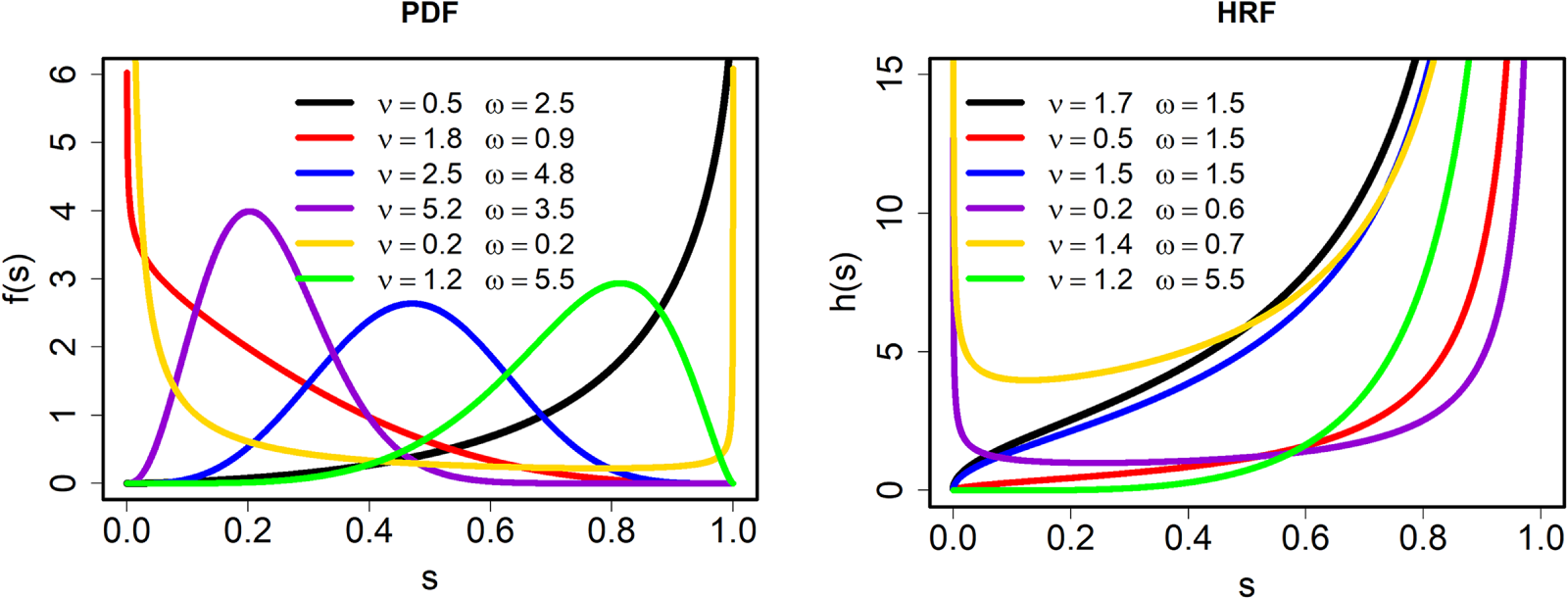
Figure 1: PDF and HRF shapes of the SUIEP distribution for different parameter values.

3  Key Statistical Characteristics

In this section, some of the basic properties of the SUIEP distribution are examined. These properties include the QF, moments (skewness, kurtosis), moment generating function, and linear expansion of PDF.

3.1 Quantile Function

The QF, which has several uses, is a crucial statistical tool. In addition to producing random numbers, it is also used to calculate the median, extreme quantiles, skewness, kurtosis, and other statistical measures. The QF of the SUIEP distribution is obtained by inverting the CDF given in Eq. (5). The inversion yields

u=sin⁡[π2[1−(1−Q(u))ν]ω],u∈(0,1).

After simplification, the QF of the SUIEP model is given by:

Q(u)=1−[1−(2πsin−1⁡(u))1/ω]1/ν,u∈(0,1).(9)

Using the expression of the QF in Eq. (9), several distributional properties can be derived, including (i) The median (second quartile), represented by Q0.5; (ii) The first quartile, represented by Q0.25; and (iii) The third quartile, represented by Q0.75. These quartiles can be used to obtain additional distributional characteristics of the SUIEP distribution. Moreover, random data sets can be generated using the QF given in Eq. (9).

3.2 Linear Representation

Linear representation in probability distribution can be defined as the linear combination of various random variables or functions. This technique can be employed to ease analysis, obtain theoretical results, and carry out computations by splitting a complex random variable into simple ones. The PDF of the SUIEP distribution can be expanded into linear form using the cos function expansion (Gradshteyn and Ryzhik [32]):

cos⁡(y)=∑l=0∞(−1)l(2l)!y2l.(10)

Utilizing the expansion (10) in the last term of the PDF of Eq. (6) gives

f(s;Φ)=∑l=0∞(−1)l(2l)!(π2)2l+1νω(1−s)ν−1[1−(1−s)ν]ω(2l+1)−1.(11)

Given the following generalized binomial expansion

(1−z)b=∑m=0∞(−1)m(bm)zm,|z|<1.(12)

Applying the binomial expansion (12) in Eq. (11) gives:

f(s;Φ)=∑l,m=0∞φl,mνω(1−s)ν(m+1)−1,(13)

where φl,m=(−1)l+m(2l)!(π2)2l+1(ω(2l+1)−1m).

3.3 Moments Measures

Moments provide information about the data’s higher-order behavior, variability, and core tendency. These are crucial for comprehending the ideas of skewness and kurtosis in environmental or financial contexts. Using PDF of Eq. (13), the qth-moment of the SUIEP distribution is found as follows:

μq′=∫01sqf(s;Φ)ds=∑l,m=0∞φl,mνω∫01sq(1−s)ν(m+1)−1ds.(14)

The integral in Eq. (14) represents a beta function, so the qth-moment of the SUIEP distribution can be expressed as follows:

μq′=∑l,m=0∞φl,mνωB(q+1,ν(m+1)),(15)

where B(.,.) is the beta function. For q = 1, in Eq. (15), the mean (μ1′) of the SUIEP distribution is produced. For q = 1, 2, the variance σ2=μ2′−(μ1′)2 of the SUIEP distribution is obtained. Other important measures, including the skewness measure (ς) defined by ς=(μ3′−3μ2′μ1′+2μ1′3)/σ3 and the kurtosis measure (κ) defined by κ=(μ4′−4μ3′μ1′+6μ1′2μ2′−3μ1′4)/σ4. To better understand the SUIEP distribution, its behavior is analyzed through both numerical data and visuals. Table 1 provides a detailed statistical summary, showing how the mean (μ1′), variance (σ2), skewness (ς), and kurtosis (κ) change as the parameters are adjusted. These shifts make it easy to evaluate the distribution’s performance. Additionally, Fig. 2 features 3D plots of these four measures, all of which were calculated and rendered using the R programming language.

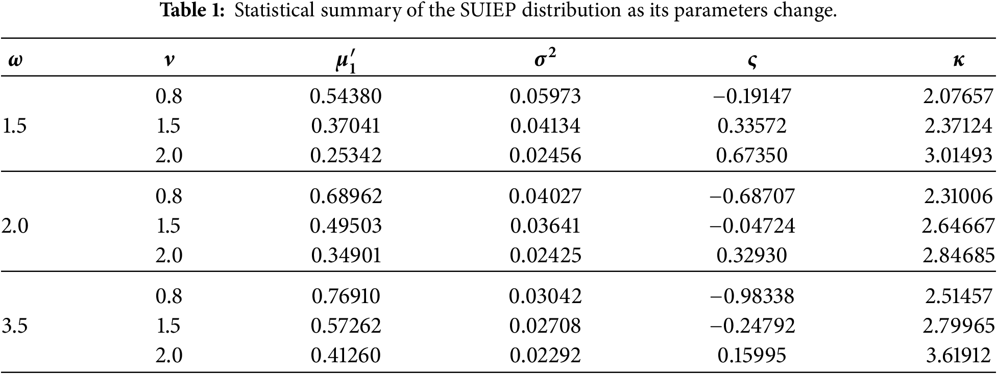
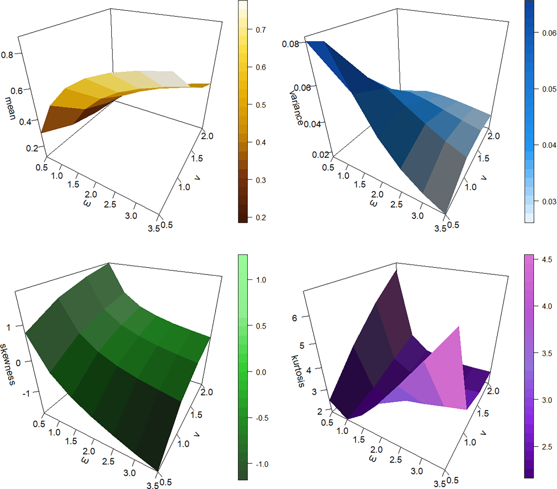
Figure 2: 3D view of the SUIEP distribution shapes.

The following observations can be made from Table 1:

1.   As ω stays the same, increasing the value of ν has a mixed effect: the values for μ1′ and σ2 decrease, while ς and κ both increase.

2.   As ν stays the same, increasing the value of ω has a mixed effect: the values for ς and σ2 decrease, while μ1′ consistently increases. The behavior of kurtosis (κ) varies; it generally increases for lower values of ν, but exhibits a non-monotonic pattern at ν=2.0.

3.   When ω and ν are kept equal and increased together, μ1′, σ2, and ς decrease, while κ increases.

4.   The SUIEP distribution is exceptionally adaptable for modeling data bounded on the unit interval [0,1]. It can handle data that is skewed to the left or right, as well as flat and peaked shapes (platykurtic and leptokurtic). Its capacity to accommodate diverse degrees of asymmetry and peakedness makes it a highly flexible tool for modeling double-bounded data.

Fig. 2 visualizes the flexibility of the SUIEP distribution, matching the results from Table 1. It is clear from the 3D plots that the distribution covers a wide range of skewness and kurtosis. This adaptability is why the PDF and HRF are so effective at fitting different types of data.

Furthermore, the MGF of the SUIEP distribution is given by

MS(t)=E(etS)=∑q,l,m=0∞tqq!φl,mνωB(q+1,v(m+1)),

where B(.,.) is the beta function.

The applicability of incomplete moments is seen in the field of econometric theory in the form of Lorenz and Bonferroni curves and in survival theory in the form of the mean residual function. The general form of the q-th incomplete moment of the SUIEP distribution is as follows:

μq′(a)=∫0asqf(s;τ)ds=∑l,m=0∞φl,mνω∫0asq(1−s)v(m+1)−1ds=∑l,m=0∞φl,mνωB(q+1,v(m+1),a),

where B(.,.,x) is the incomplete beta function. Based on this function, Fig. 3 displays the Lorenz and Bonferroni curves to show how the SUIEP distribution measures data inequality under different parameter values.

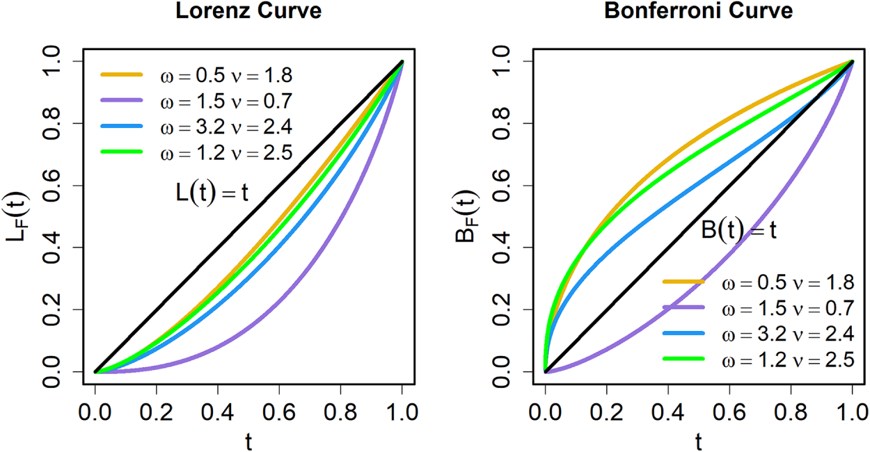
Figure 3: Measuring SUIEP distribution inequality: Lorenz vs. Bonferroni.

As demonstrated in Fig. 3, changing the parameter values significantly alters the trajectory of both inequality curves. While the gold curve tracks closely to the 45-degree line (indicating balance), the purple and green curves highlight a shift toward greater disparity. However, the Bonferroni curves offer a more nuanced view of the lower distribution. Here, the green curve’s steeper descent reveals that the poorest groups are disproportionately affected. Ultimately, this comparison illustrates that the Bonferroni curve provides a deeper granularity for analyzing bottom-heavy inequality than the standard Lorenz plot.

3.4 Stress-Strength Reliability

The stress-strength (S-S) reliability is a key performance parameter in the assessment of the operational integrity of a system. It is defined as the probability that the strength of a system (S1) is higher than the stress (S2) to which the system is exposed, i.e., ℜ=P(S2<S1). If the stress (S2) exceeds the strength (S1), the system fails. Though a conventional engineering parameter, the S-S reliability is being used in biological modeling and financial risk assessment. Let the independent random variables S1 and S2 represent the strength and stress components, respectively, both following the SUIEP distribution. Specifically, suppose S1 with the PDF f(s1) with parameters (ω1,ν) and suppose S2 with the PDF f(s1) with parameters (ω2,ν). The S-S reliability is derived as follows:

ℜ=∫01π2νω1(1−s1)ν−1[1−(1−s1)ν]ω1−1cos⁡[π2[1−(1−s1)ν]ω1]sin⁡[π2[1−(1−s1)ν]ω2]ds1.(16)

To obtain ℜ, we apply the cos expansion from Eq. (10) along with the following sine expansion

sin⁡(k)=∑n=0∞(−1)n(2n+1)!k2n+1.(17)

Then, the S-S reliability ℜ, is given by

ℜ=νω1∑j1,j2=0∞(−1)j1+j22j1!(2j2+1)!(π2)2j1+2j2+2∫01(1−s1)ν−1[1−(1−s1)ν]ω1(2j1+1)+(2j2+1)ω2−1ds1.(18)

Using the transformation y=(1−s1)ν, in Eq. (18), the S-S reliability can be expressed as:

ℜ=∑j1,j2=0∞(−1)j1+j2ω12j1!(2j2+1)!(π2)2j1+2j2+21ω1(j1+1)+(2j2+1)ω2.

It is hard to understand the definitive formula for reliability on its own. To make the results clearer, Fig. 4 shows the SUIEP distribution visually. This makes it much easier to understand how reliability actually works.

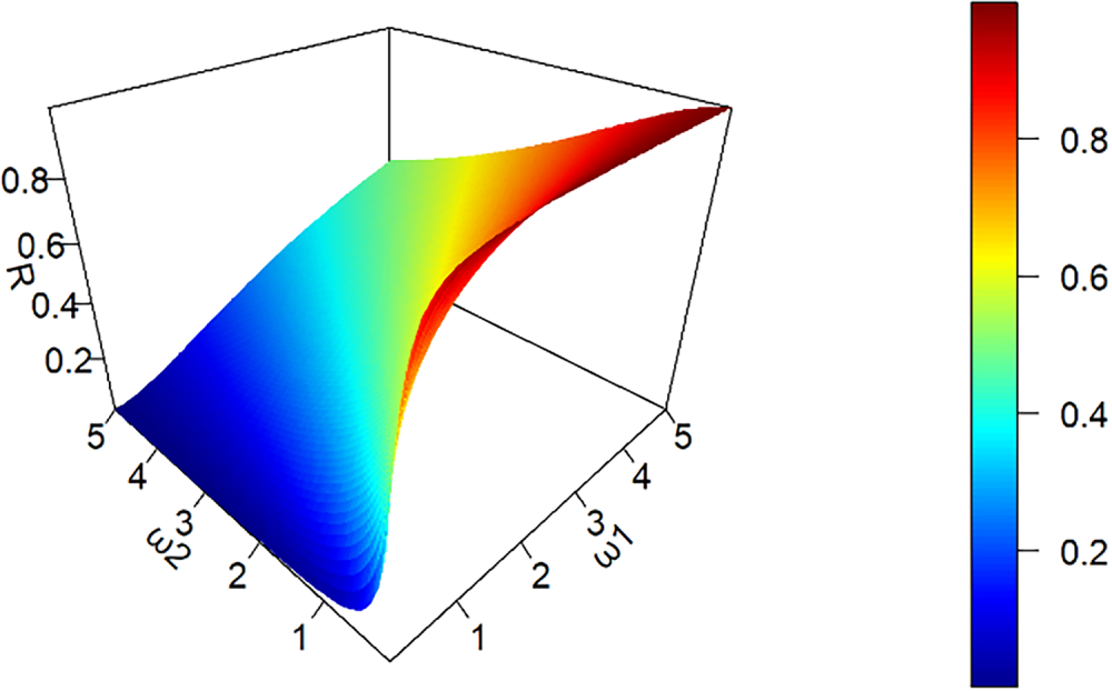
Figure 4: 3D reliability surface for the SUIEP distribution.

There are changes in the reliability of the SUIEP distribution, which can be seen in Fig. 4. Visual inspection of Fig. 4 demonstrates this monotonic behavior clearly: the reliability increases as ω1 increases, whereas it decreases as ω2 increases. Beyond demonstrating this monotonic behavior, the surface reveals the sensitivity of ℜ to parameter shifts. The steep gradient highlights that ℜ is highly sensitive to small simultaneous variations at lower parameter values. From a practical perspective, this 3D profile allows engineers to visually determine the precise strength threshold required to withstand a given stress level in order to maintain a specific target ℜ.

3.5 Entropy Measures

Entropy serves as a measure of the average information content or uncertainty inherent in a random variable’s distribution. Higher entropy values reflect increased data uncertainty and randomness. Consequently, the concept of entropy is essential across a wide array of fields, including physics, probability and statistics, economics, and communication theory. The Rényi entropy (χ1) measure, suggested by Rényi [33], is defined by:

χ1=1(1−p)log⁡[∫01(f(s;τ))pds],p>0,p≠1.(19)

Hence, the integral of Eq. (19) is obtained by using the PDF given in Eq. (6) as follows:

I=(π2νω)p∫01(1−s)p(ν−1)[1−(1−s)ν]p(ω−1)cosp⁡[π2[1−(1−s)ν]ω]ds.(20)

To obtain χ1, we apply cosine expansion given in Eqs. (10)–(20):

cosp⁡[π2[1−(1−s)ν]ω]=1+∑i1=1∞(pi1)[1−(1−s)ν]2ωi1{∑i3=0∞Λi3[1−(1−s)ν]2ωi2}i1,(21)

where Λi3=(−1)i3+1(0.5π)2(i3+1)2(i3+1)!, since i1≥1. we can use the following power series (presented by Gradshteyn and Ryzhik [32])

(∑k=0∞ckzk)q=∑k=0∞fkzk,f0=c0q,fk=(c0m)−1∑k=1m(kq−m+k)ckfm−k,m≥1,

in Eq. (21) leads to

cosp⁡[π2[1−(1−s)ν]ω]=1+∑i1=1∞∑i3=0∞Λi1,i3∗[1−(1−s)ν]2ω(i1+i3),(22)

where Λi1,i3∗=(pi1)Λi3. Substituting Eq. (22) in the integral (20), we get

I=(π2νω)p[1νB(p(ν−1)+1ν,p(ω−1)+1)]+(π2νω)p∑i1=1∞∑i2=0∞Λi1,i2∗[1νB(p(ν−1)+1ν,p(ω−1)+2ω(i1+i2)+1)].(23)

Hence, the Rényi entropy of the SUIEP distribution is obtained by inserting Eq. (23) in Eq. (19) as follows:

χ1=1(1−p)log⁡[(π2νω)p[1νB(p(ν−1)+1ν,p(ω−1)+1)]+(π2νω)p∑i1=1∞∑i2=0∞Λi1,i2∗[1νB(p(ν−1)+1ν,p(ω−1)+2ω(i1+i2)+1)]].(24)

Additionally, following Tsallis [34], the Tsallis entropy for the SUIEP distribution is determined as follows

χ2=1(p−1)[1−∫01(f(s;τ))pds],p>0,p≠1.(25)

Inserting integral (23) in expression (25), the Tsallis entropy for the SUIEP distribution is given by

χ2=1(p−1)[1−(π2νω)p[1νB(p(ν−1)+1ν,p(ω−1)+1)]−(π2νω)p∑i1=1∞∑i2=0∞Λi1,i2∗[1νB(p(ν−1)+1ν,p(ω−1)+2ω(i1+i2)+1)]].

The entropy expressions in (24) and (25) are difficult to simplify, so numerical methods were used to solve them across various parameter values. Table 2 presents these core measurements, while Fig. 5 provides a visual representation of the uncertainty levels within the SUIEP distribution. All calculations and visualizations were performed using the R programming language.

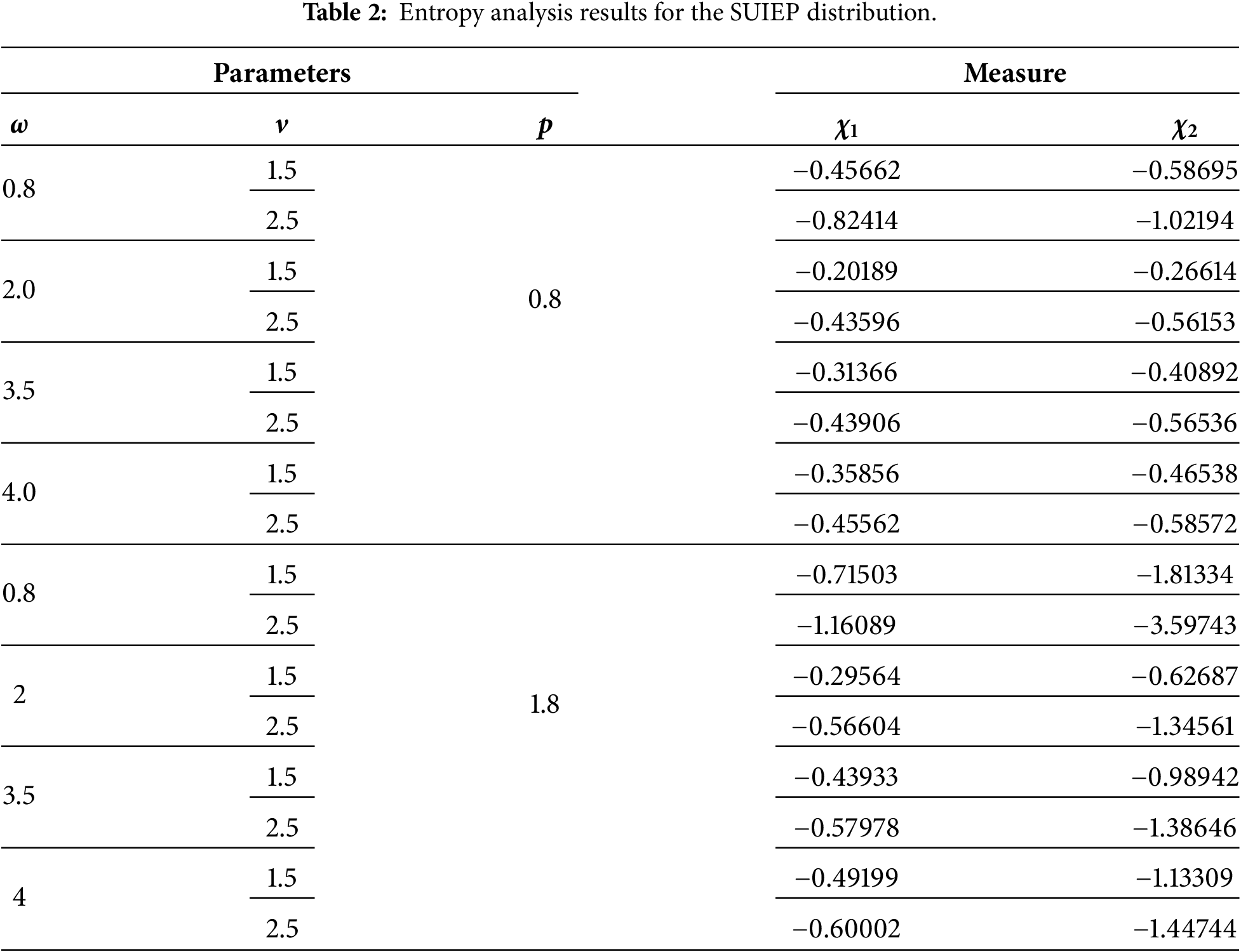
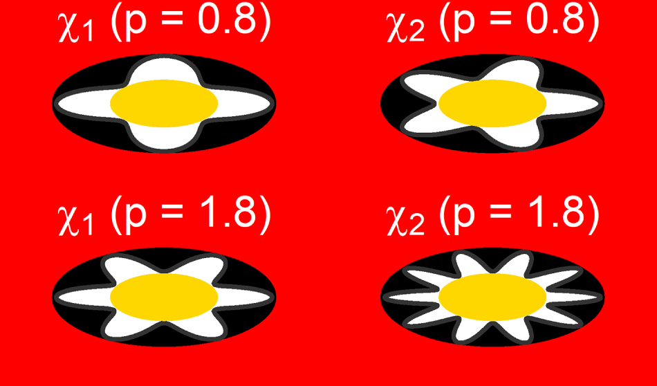
Figure 5: Visualizing uncertainty in SUIEP distribution entropy.

Based on numerical results in Table 2, the entropy values show that:

1.   The values of χ1 are consistently greater than the values of χ2 across all parameter combinations.

2.   If p and ω stay the same, increasing ν makes the entropy level decrease.

3.   If p and υ remain constant, increasing ω does not result in a strictly monotonic change in the entropy level. Instead, both χ1 and χ2 initially increase when ω shifts from 0.8 to 2.0, before decreasing again at higher values of ω (3.5 and 4.0).

4.   If ν and ω stay the same, increasing p makes the entropy level decrease.

The visual breakdown in Fig. 5 uses white to highlight uncertainty and yellow for average entropy. A smaller white area indicates a more favorable outcome with less uncertainty, a balance driven by the p value. This visualization clearly demonstrates that measure χ1 is more effective than measure χ2 at p = 0.8 and 1.8, directly supporting the numerical data in Table 2.

4  Maximum Likelihood Estimation

Parameter estimation for the SUIEP model is performed here using the maximum likelihood method. Let ω^ and ν^ denote the maximum likelihood estimate (MLE) of the parameters ω and ν, respectively. Let s1, s2, …, s1, be a random sample of size n from the density f(s;Φ). The likelihood function for the parameters ω and ν is formulated as follows:

L(Φ)=[π2νω]n∏l=1n(1−sl)ν−1[1−(1−sl)ν]ω−1cos⁡[π2[1−(1−sl)ν]ω].(26)

The log-likelihood function for the parameters ω and ν is formulated as follows:

ℓ(Φ)∝nlog⁡(νω)+(ν−1)∑l=1nlog⁡(1−sl)+(ω−1)∑l=1nlog⁡[1−(1−s)ν]+∑l=1nlog⁡{cos⁡[π2[1−(1−sl)ν]ω]}.(27)

From Eq. (27), the partial derivatives with respect to the parameters ω and ν are obtained as follows:

∂ℓ(Φ)∂ν=nν+∑l=1nlog⁡(1−sl)+πω2∑l=1n(1−sl)νlog⁡(1−sl)[1−(1−sl)ν]ω−1tan⁡[π2[1−(1−sl)ν]ω]−∑l=1n(ω−1)log⁡(1−sl)[(1−sl)−ν−1],(28)

and,

∂ℓ(Φ)∂ω=nω+∑l=1nlog⁡[1−(1−s)ν]−π2∑l=1n[1−(1−sl)ν]ωlog⁡[1−(1−sl)ν]tan⁡[π2[1−(1−sl)ν]ω].(29)

Eqs. (28) and (29) have implicit estimators for ω^ and ν^ when the right-hand side is set to zero. Since there is no analytical solution for this system, the estimator values are repeatedly obtained using the Nelder-Mead method as a numerical optimization technique.

5  Bayesian Estimation

The maximum likelihood methodology is popularly employed; however, closed form solutions are difficult to derive in complicated lifetime distributions, and it might be inefficient with small sample sizes. Bayesian inference offers a robust alternative that combines prior knowledge with likelihood to generate parameter distributions. Bayesian estimates (BEs) from the Markov Chain Monte Carlo (MCMC) technique will be highly effective for the current model.

Here, the Bayes’ estimators have been obtained on the basis of the squared error loss function (SELF), the weighted squared error loss function (WSELF), and the minimum expected loss function (MLF). The SELF is the most popularly used symmetric loss function. The SELF implies that the Bayes estimator is the posterior mean for each parameter, which minimizes the posterior risk as it minimizes the expected square of the deviation of the estimator from the true value.

The BE of the parameters Φ≡(ω,ν)T under SELF, represented by Φ^SELF, is given by:

Φ^SELF=E(Φ∣s_)=∫0∞∫0∞ΦΠ(Φ∣s_)dωdν.

The main purpose of the MLF is to find out which estimator gives the minimum value for the expected value of a previously chosen loss function [35]. Within the MLF approach, the BE of Φ can be written

Φ^MLF=E(Φ−1∣s_)E(Φ−2∣s_)=∫0∞∫0∞Φ−1Π(Φ∣s_)dωdν∫0∞∫0∞Φ−2Π(Φ∣s_)dωdν.

The WSELF assigning equal weight to overestimation and underestimation errors of equal magnitude (see [36,37]). The WSELF enables the weighting of errors according to particular values of the parameter and is represented as:

Φ^WSELF=E(Φ−1∣s_)−1=[∫0∞∫0∞Φ−1Π(Φ∣s_)dωdν]−1.

The BE for parameters Φ≡(ω,ν) is considered under gamma priors. We choose the gamma priors since the support of the distribution is the set of positive real numbers, which fits the domain of the parameters of the SUIEP distribution. Also, the gamma distribution significantly simplifies computations. The independent joint gamma prior density of parameters is defined as follows:

π(Φ)∝e−(ωβ1+νβ2)να2−1ωα1−1,ν,ω>0;βi,αi>0;i=1,2.(30)

Here βi,αi,i=1,2 are the hyperparameters. The joint posterior density function is obtained by multiplying the joint prior distribution given in Eq. (30) by the likelihood function in Eq. (26), dropping the normalizing constant.

π(Φ∣s_)∝νn+α2−1ωn+α1−1exp⁡{−ν[β2−∑l=1nln⁡(1−sl)]}exp⁡{−ω[β1−∑l=1nln⁡(1−(1−sl)ν)]}×∏l=1ncos⁡[π2(1−(1−sl)ν)ω].(31)

Conditional posterior densities of ω and ν are derived from the joint posterior density (31) as given below:

M1(ω∣ν,s_)∝ωα1+n−1e−ω[β1−∑l=1nln⁡[1−(1−sl)ν]]∏l=1ncos⁡[π2[1−(1−sl)ν]ω],(32)

and,

M2(ν∣ω,s_)∝νn+α2−1exp⁡{−ν[β2−∑l=1nln⁡(1−sl)]}×exp⁡{ω∑l=1nln⁡[1−(1−sl)ν]}∏l=1ncos⁡[π2[1−(1−sl)ν]ω].(33)

Eqs. (32) and (33) can’t be solved analytically, so numerical integration methods are needed to solve them. To manage the complex posterior density, we implement the MCMC methodology via R software, utilizing the Metropolis-Hastings (M-H) algorithm for sampling and Bayesian estimation. For the simulation study, the hyperparameters are determined through the method of moments as described in [38], where the mean and variance of the gamma priors are matched with the moments estimated from the MLE results. This approach enables the explicit calculation of the hyperparameters as follows:

αi=(N−1∑d=1NΦ^id)2(N−1)−1∑d=1N(Φ^id−N−1∑d=1NΦ^id)2,βi=N−1∑d=1NΦ^id(N−1)−1∑d=1N(Φ^id−N−1∑d=1NΦ^id)2,

where d represents sample repeats. Conversely, for the real-world datasets where no prior historical information or sample repeats exist, non-informative objective priors with αi=βi=0.0001 are directly adopted to ensure entirely data-driven estimation and eliminate any prior subjective bias.

5.1 M–H Algorithm

Since the Bayes estimators for ω^ and ν^ derived from Eqs. (32) and (33) do not conform to any standard analytical statistical distributions, an M-H sampler within the MCMC framework is utilized. This algorithm offers a reliable computational approach by generating iterative samples through symmetric normal proposal distributions [39]. The precise computational steps of the procedure are outlined below:

1.   Initial Configuration: Begin the process by assigning the preliminary states ω(0) and ν(0) to initialize the parameter chains. Set the iteration counter to x=1 to start the sequence.

2.   The Sampling Procedure for ω: For each iteration x, propose a new candidate ω∗ by sampling from the Gaussian proposal distribution N(ω(x−1),σ2(ω)). The acceptance or rejection of this candidate is determined through the following sub-steps:

•   Probability Calculation: Compute the M-H acceptance ratio ℵ1 using the target full conditional distribution ratio:

ℵ1=min{1,C1(ω∗∣ν(x−1),s_)C1(ω(x−1)∣ν(x−1),s_)}.(34)

•   Stochastic Testing: Draw a random value u1 from the standard uniform distribution U(0,1).

•   State Update: Compare the uniform draw against the acceptance ratio. If u1<ℵ1, accept the candidate and set the current state to ω(x)=ω∗; otherwise, reject the candidate and maintain the previous state by setting ω(x)=ω(x−1).

3.   The Sampling Procedure for ν: Similarly, propose a new candidate ν∗ from its respective proposal distribution N(ν(x−1),σ2(ν)). Compute the corresponding acceptance ratio ℵ2 as follows:

ℵ2=min{1,C2(ν∗∣ω(x),s_)C2(ν(x−1)∣ω(x),s_)}.(35)

Draw a random value u2 from U(0,1). If u2<ℵ2, update the state to ν(x)=ν∗; otherwise, set ν(x)=ν(x−1).

4.   Iteration and Final Output: Increment the iteration counter x=x+1 and repeat Steps 2 and 3 sequentially for a total of N iterations.

6  Distributions and Applied Statistical Modeling

The effectiveness of the SUIEP distribution is assessed by benchmarking it against a set of well-known unit distributions using two real-world datasets: COVID-19 daily mortality rates and unmanned aerial systems detection efficiency data. The distributions considered for comparison are the UIEP distribution [31], unit Weibull (UW) distribution [40], unit Gompertz (UG) distribution [41], unit Gumbel (UGu) distribution [42], truncated exponentiated-exponential (TEE) distribution [43], Kavya-Manoharan unit-Gompertz (KMUG) distribution [44], and sine power unit inverse Lindley (SPUIL) [45] distribution.

The BE is obtained for the proposed SUIEP distribution, whereas MLE was provided for all competing models. To assess the goodness-of-fit, eight criteria were considered, covering four information-based measures: Akaike information criterion (ε1), Bayesian information criterion (ε2), corrected Akaike information criterion (ε3), and Hannan-Quinn information criterion (ε4), as well as three statistical test statistics: Anderson-Darling (ε5), Cramér-von Mises (ε6), and Kolmogorov-Smirnov (ε7), along with the p-value associated with the Kolmogorov-Smirnov test (ε8). Lower values of ε1−ε7 and a higher value of ε8 reflect a better distributional fit. From a decision-theoretic background, while an asymmetric loss function (MLF) is conceptually valuable in public health and security contexts to penalize underestimation more severely, the empirical applications in this study are conducted under the standard symmetric SELF framework. This selection serves as a reliable baseline benchmark to provide a direct and well-established statistical interpretation of the SUIEP distribution parameters.

(a)   COVID-19 Mortality Rate Data

The first application utilizes a 36-day dataset of COVID-19 daily mortality rates (measured per 100,000 population) from Saudi Arabia, covering the period from 22 July to 26 August 2021 [46]. This record provides a real-world basis for evaluating the model’s fit under specific health-related trends. The observed values are as follows: 0.2375, 0.2962, 0.2167, 0.2752, 0.2353, 0.2347, 0.1951, 0.2140, 0.2329, 0.2711, 0.2126, 0.2314, 0.1924, 0.2113, 0.2683, 0.2487, 0.2674, 0.1716, 0.2666, 0.2091, 0.2278, 0.1706, 0.2271, 0.1890, 0.2077, 0.2452, 0.1319, 0.2259, 0.1504, 0.1879, 0.1689, 0.2063, 0.2249, 0.1686, 0.1310, 0.1497.

Based on the data listed above, Fig. 6 provides a comprehensive graphical overview of the COVID-19 mortality rate’s basic descriptive metrics.

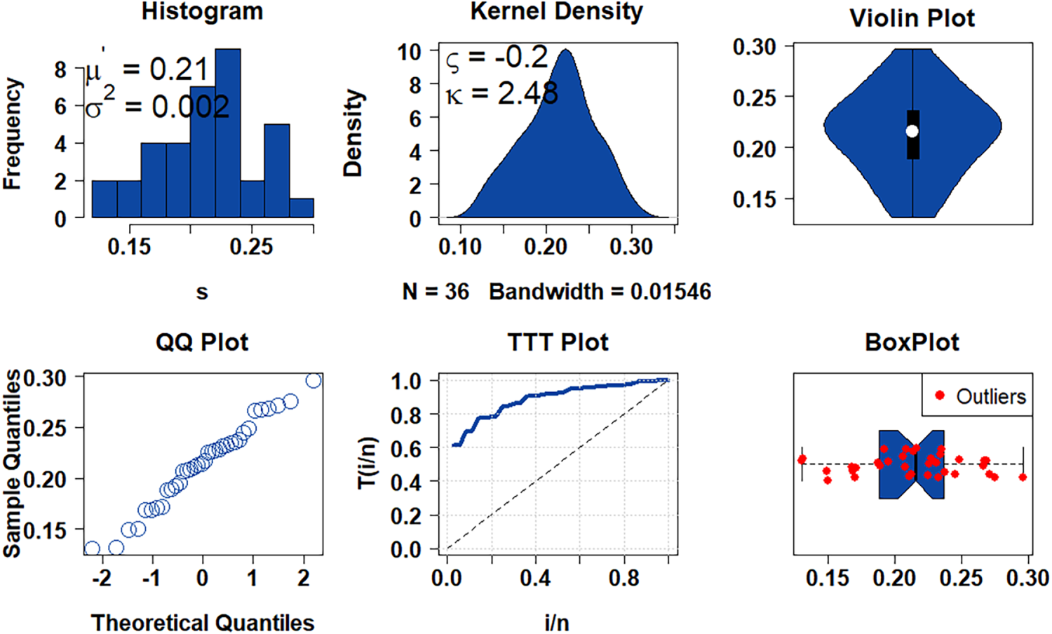
Figure 6: Statistical diagnostic plots for COVID-19 mortality rate data.

The distributional properties of the data are explored in Fig. 6, where the quantile-quantile (QQ) and box plots reveal departures from normality and identify outliers (marked by red rings). The asymmetrical nature of the data is further evidenced by the PDF visualization, while the total test time (TTT) plot exhibits a concave pattern, indicating an increasing empirical hazard rate. This supports the application of the SUIEP distribution, which flexibly accommodates increasing HRF behaviors alongside other shapes. Building on this preliminary analysis, Table 3 summarizes the MLEs and their corresponding standard errors (S.E.s) for all competing models. For the SUIEP distribution specifically, BEs are calculated under the SELF using hyperparameters (αj,βj=0.0001,j=1,2).

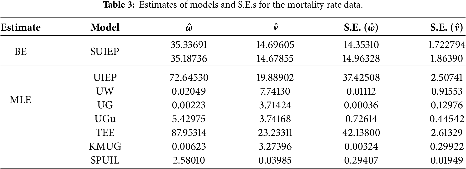
Table 3 exhibits lower standard errors for the Bayesian estimates compared to the MLEs, showing a performance trend on the empirical data that aligns with the pattern observed in the simulation study. This is supported by Fig. 7, where MCMC plots verify the stability of these parameters. Finally, Fig. 8 uses log-likelihood and contour plots to show how effectively these estimators work with mortality rate data.

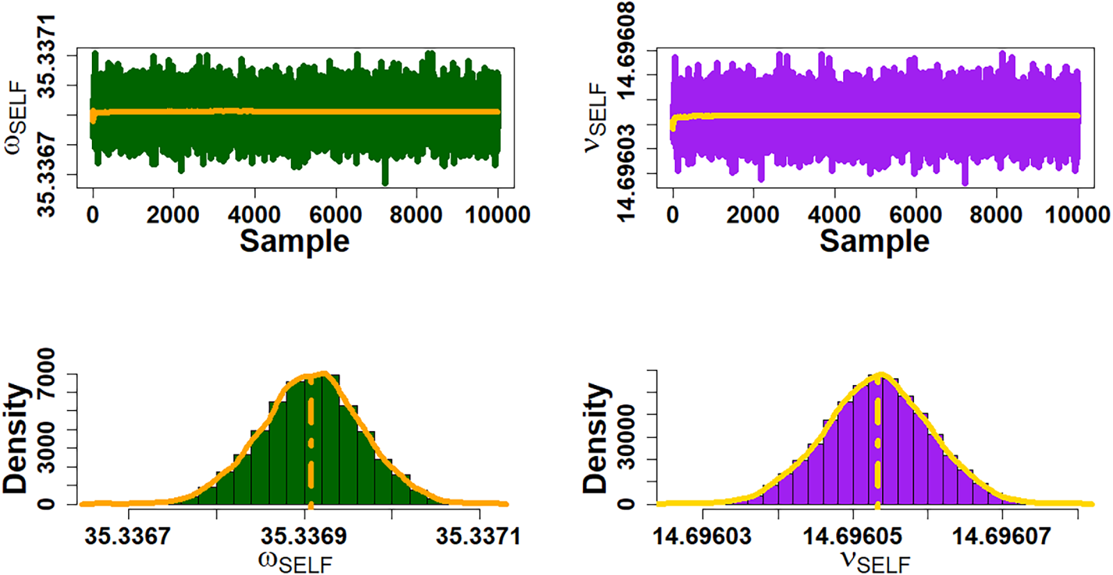
Figure 7: MCMC graphs of mortality rate data for ω and ν.

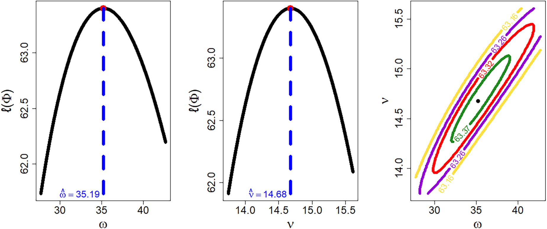
Figure 8: Likelihood analysis for contour and profile plots for COVID-19 mortality data.

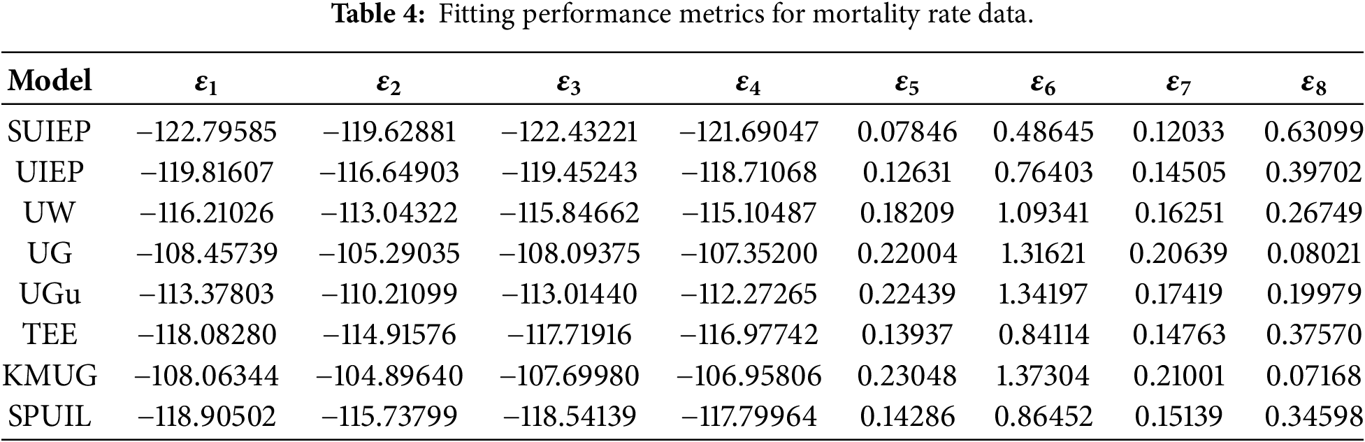
These figures help validate the methods used to estimate parameters for mortality rate data. Fig. 7 shows the BE results, where the MCMC chains converge steadily. The histograms for the 10,000 values show that the parameter distributions are normal and symmetric. Additionally, the plots in Fig. 8 confirm that the MLEs successfully identify the best values for fitting the SUIEP distribution. Together, these visuals prove that both estimation methods work effectively. Table 4 also includes goodness of fit measurements ε1, ε2, ε3, ε4, ε5, ε6, ε7, and ε8. Since all candidate models are two-parameter distributions evaluated on the same sample size, the parameter-penalty terms in the formulas for ε1,ε2,ε3, and ε4 are identical, resulting in mathematically constant differences between these metrics across all models.

A comparative analysis of the SUIEP distribution and competing models is depicted in Figs. 9 and 10. Specifically, Fig. 9 showcases the empirical PDF (EPDF) and empirical CDF (ECDF) fits, while Fig. 10 utilizes probability-probability (P-P) plots to confirm the distributional accuracy using the mortality rate data.

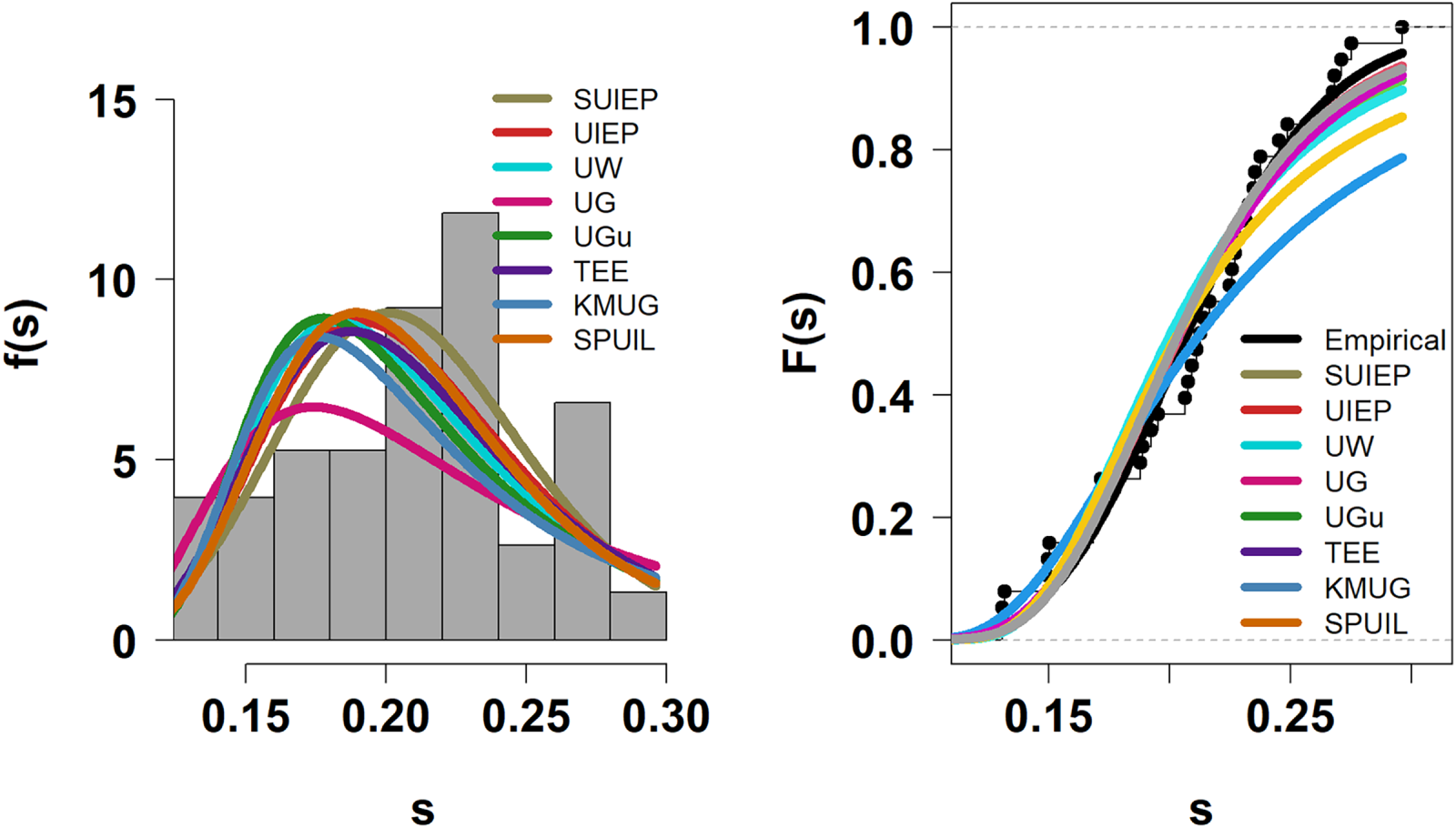
Figure 9: EPDF and ECDF visualizations for COVID-19 mortality data.

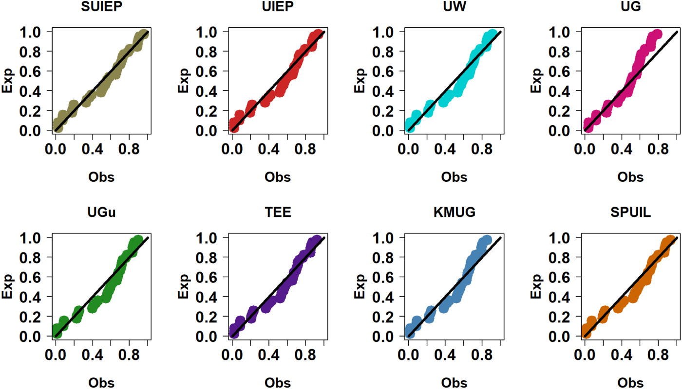
Figure 10: P-P plots comparing different mortality rate data distributions.

(b)   Air defence Monitoring Data

The dataset employed in this study is based on monthly Unmanned Aerial Systems (UAS) sighting counts derived from official operational records published by the U.S. Federal Aviation Administration (FAA) at https://www.faa.gov/uas/resources/public_records/uas_sightings_report. Covering the period from January 2021 to February 2025 (N=50 observations), the raw monthly sighting counts were normalized by dividing each value by the maximum observed count to scale them into (0,1) for unit-interval modeling. Analyzing such proportions provides a statistically rigorous foundation for developing advanced defense frameworks and precision-based monitoring systems aimed at maintaining air defense sovereignty. The resulting 50 normalized observations are: 0.704887, 0.416034, 0.717348, 0.494136, 0.485496, 0.265854, 0.726284, 0.069275, 0.284736, 0.367434, 0.529289, 0.255940, 0.584703, 0.747535, 0.236573, 0.438216, 0.078951, 0.346456, 0.141450, 0.685592, 0.368019, 0.673375, 0.533359, 0.587263, 0.242077, 0.173106, 0.439750, 0.239029, 0.503798, 0.356013, 0.407615, 0.657437, 0.404920, 0.199932, 0.233185, 0.415147, 0.406094, 0.456606, 0.352986, 0.462306, 0.350980, 0.450283, 0.522406, 0.245437, 0.341617, 0.396632, 0.480016, 0.285083, 0.419322, 0.450749. Based on the data listed above, Fig. 11 provides a comprehensive graphical overview of the air defense monitoring’s basic descriptive metrics.

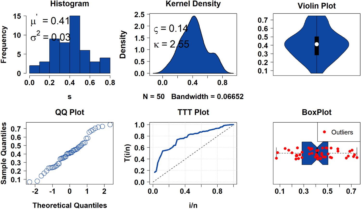
Figure 11: Statistical diagnostic plots for air defence monitoring data.

Fig. 11 explores the data’s properties, with QQ and box plots showing non-normal patterns and outliers (red rings). The PDF and TTT plots confirm the data’s asymmetry and show that the SUIEP distribution provides the most adequate fit for the HRF behavior among the considered models. Table 5 then lists the MLEs and SEs for all models, including the BEs for the SUIEP distribution calculated using hyperparameters (αj,βj=0.0001,j=1,2).

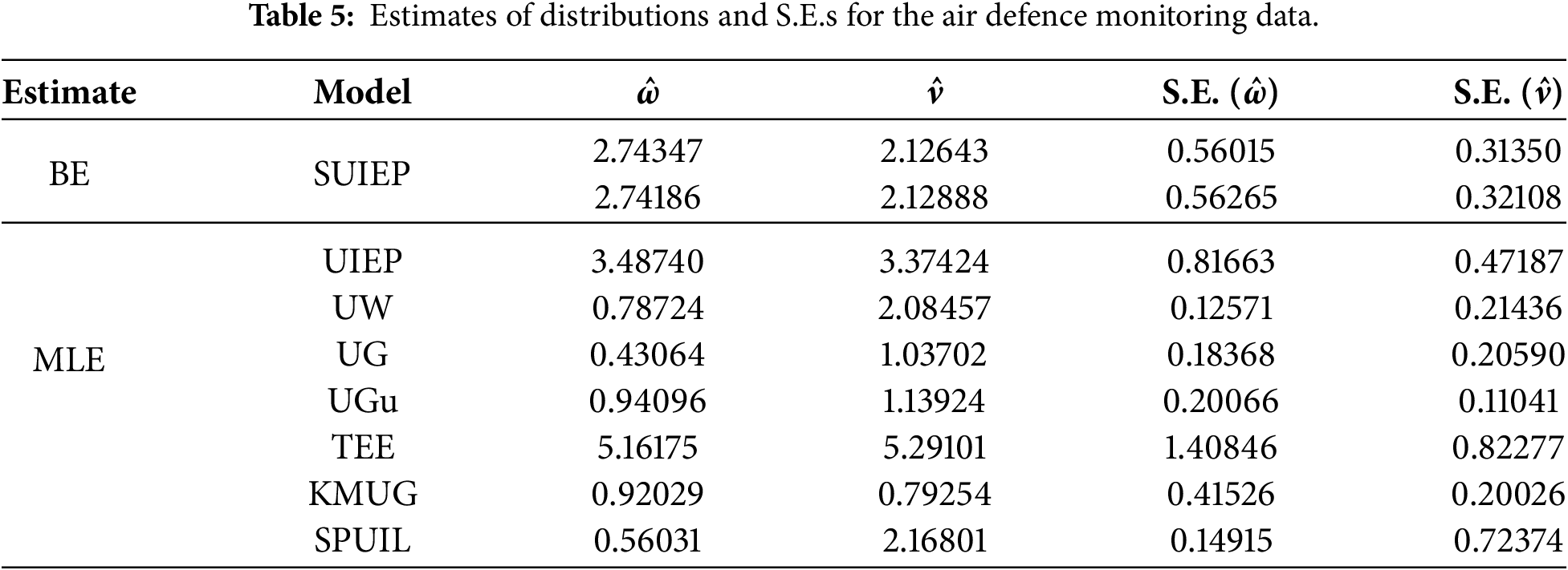
Table 5 confirms that the BE method is the best for estimating SUIEP parameters, matching the simulation results. Fig. 12 proves that the parameters are stable through MCMC plots, while Fig. 13 shows that these estimators work very well for air defense monitoring data.

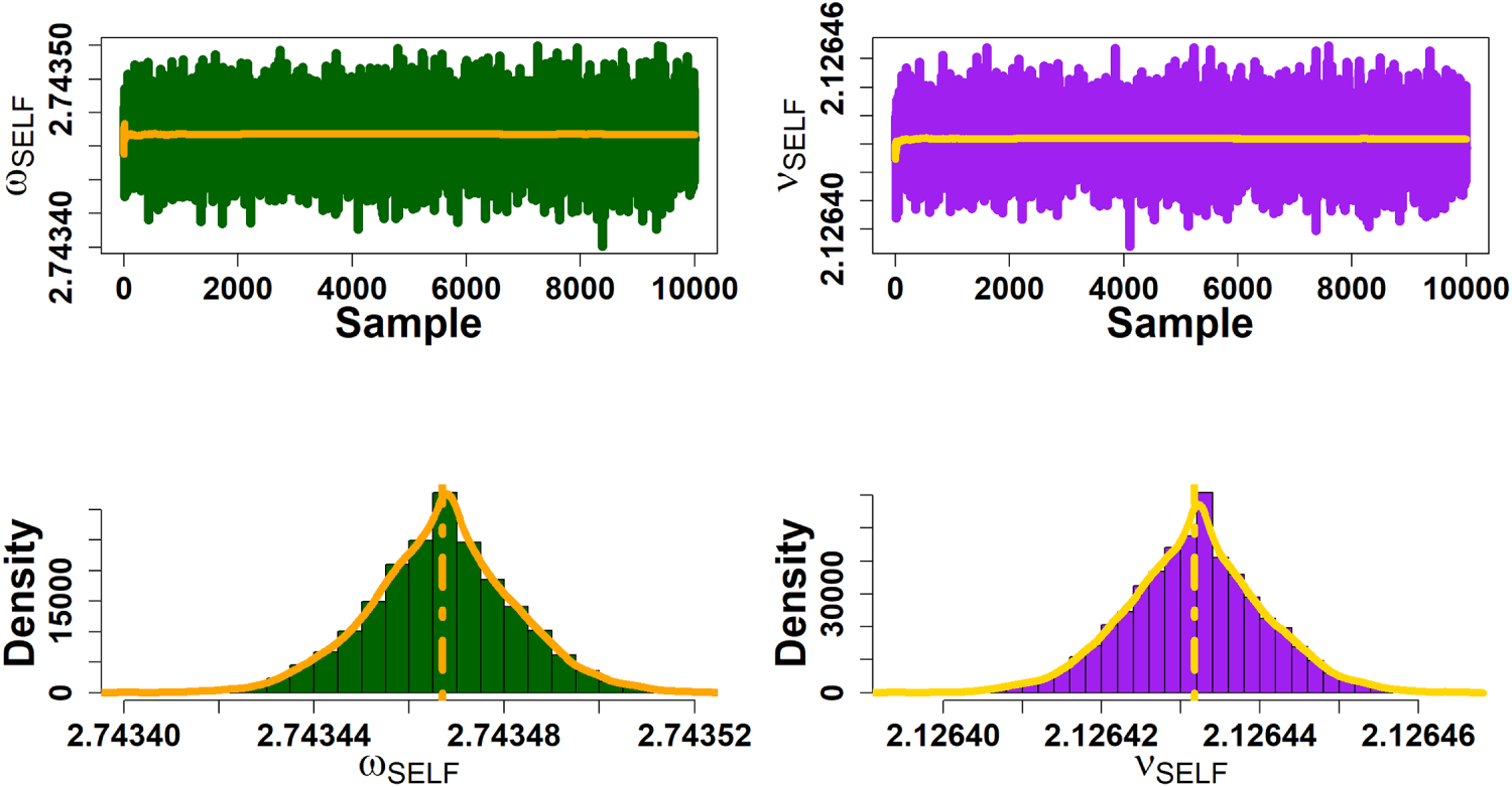
Figure 12: MCMC diagnostics of air defence monitoring data for ω and ν.

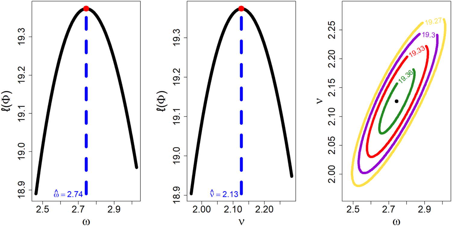
Figure 13: Likelihood analysis for contour and profile plots for air defence monitoring data.

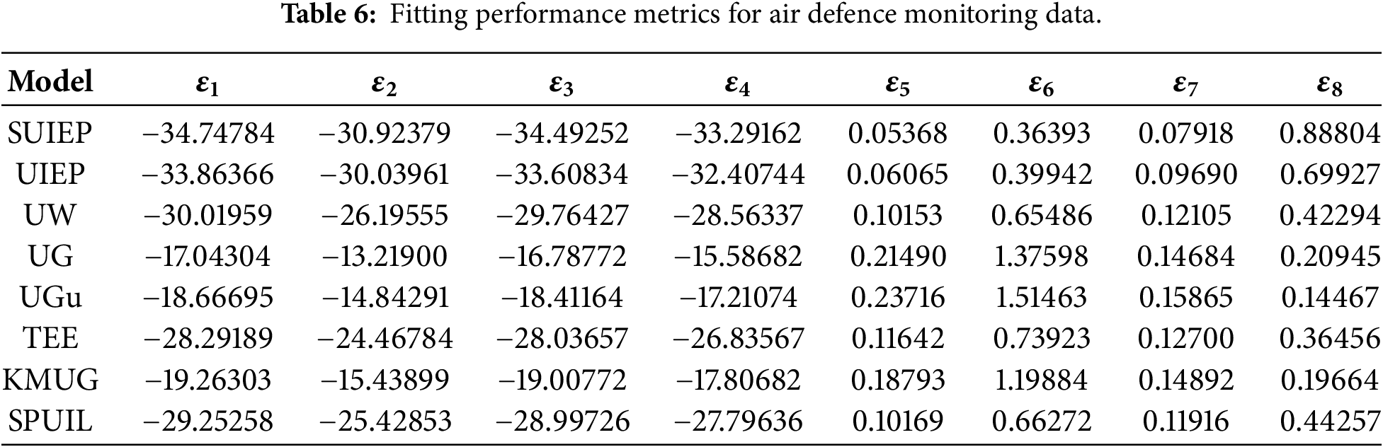
These figures validate the estimation methods used for the air defence data. Fig. 12 shows stable MCMC results for the SUIEP distribution, with histograms reflecting a symmetric, normal distribution. Fig. 13 confirms that the MLEs effectively find the best parameters for this model. Overall, these visuals and the measurements in Table 6 (ε1–ε8) prove that our proposed approach is more effective than the other distributions.

To see how the SUIEP distribution performs compared to others, visual tools were used with air defence monitoring data. Fig. 14 shows the EPDF and ECDF comparisons, while Fig. 15 uses P-P plots to verify the fit. These visuals confirm that the SUIEP distribution fits the data better than the competing distributions.

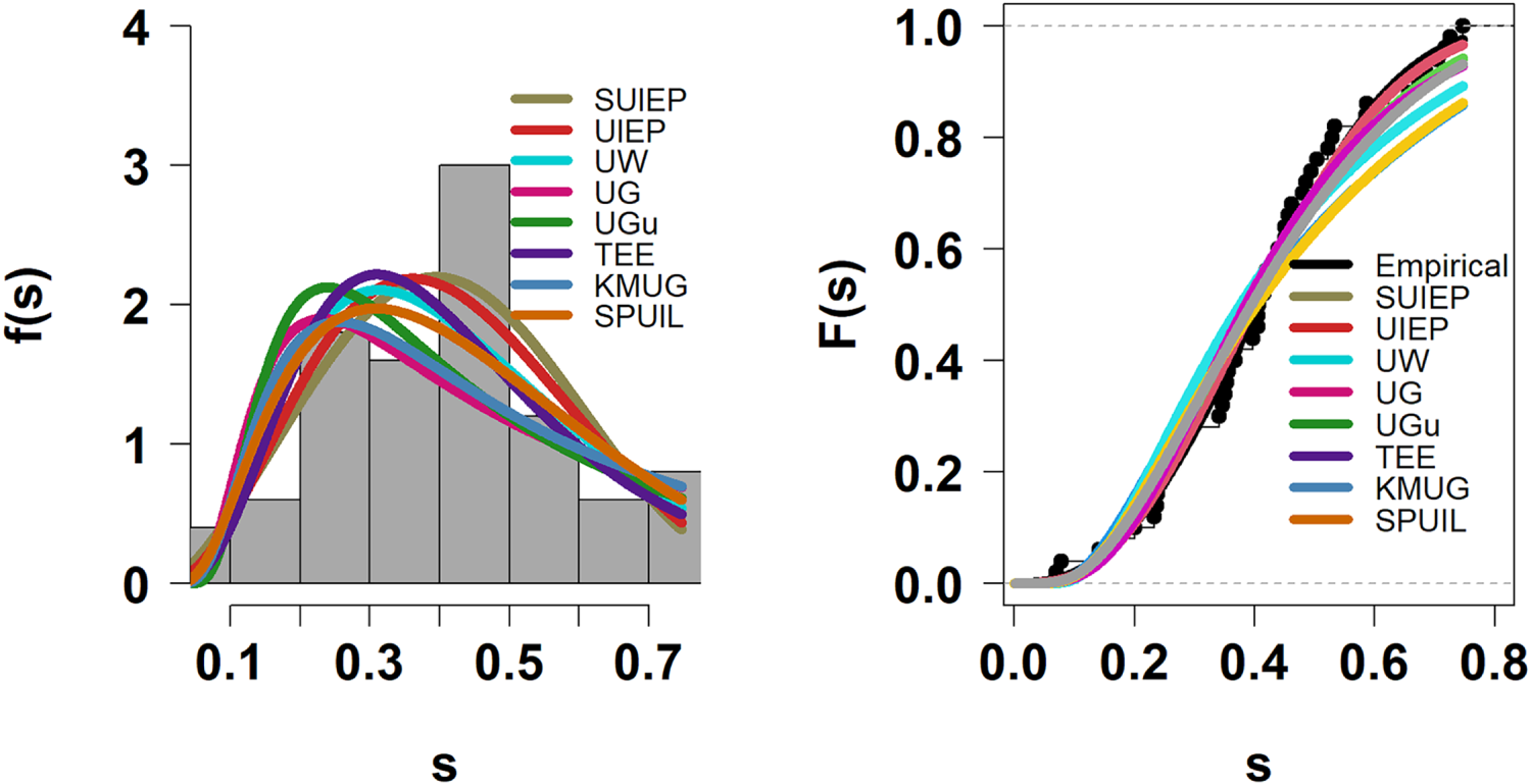
Figure 14: EPDF and ECDF visualizations air defence monitoring data.

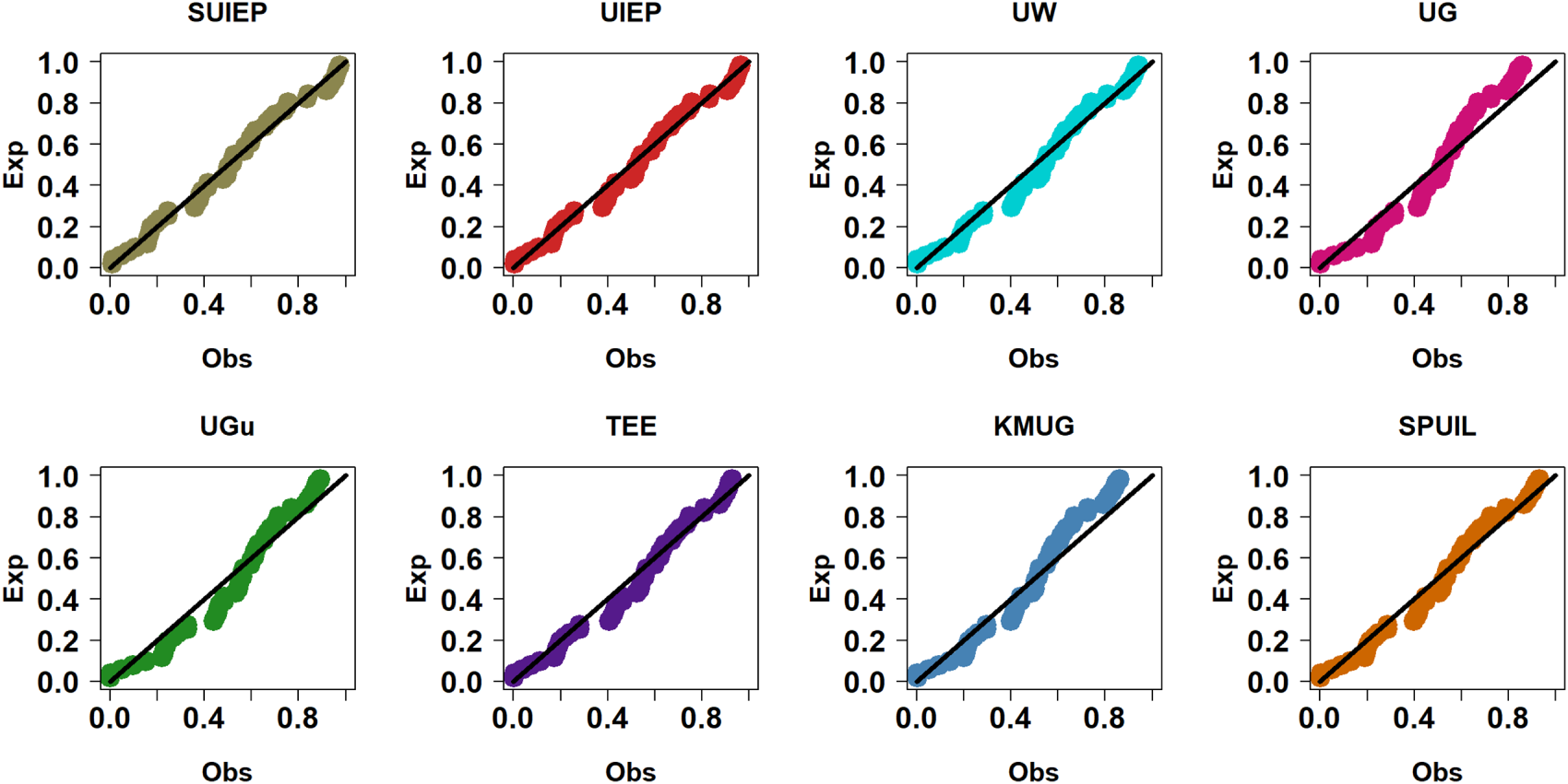
Figure 15: P-P plot diagnostics for air defence monitoring data distributions.

7  Monte Carlo Simulation

A Monte Carlo simulation with 1000 replications was designed to assess the performance of MLE and BE for the SUIEP distribution. In this study, the Bayesian approach is executed using SELF, WSELF, and MLF under gamma priors. We considered a variety of sample sizes, specifically n = 20, 50, 80, 100, and 120, and used absolute bias (A.B.) and mean squared error (M.S.E.) measures as the primary evaluation criteria. To obtain the BEs, an MCMC of 10,000 samples was generated, discarding the first 2,000 observations as a burn-in period. The effectiveness of the distribution is examined through the following specific parameter sets:

Set1 = (ω=1.5,ν=2) Set2 = (ω=2,ν=1.5)

Set3 = (ω=1.5,ν=1.5) Set4 = (ω=2.4,ν=2.4)

To execute the estimation procedures, R (version 4.5.2) was used along with the ‘maxLik’ package for MLE and the ‘MCMCpack’ package for BE. The comprehensive results are detailed in Table 7 and illustrated in Fig. 16.

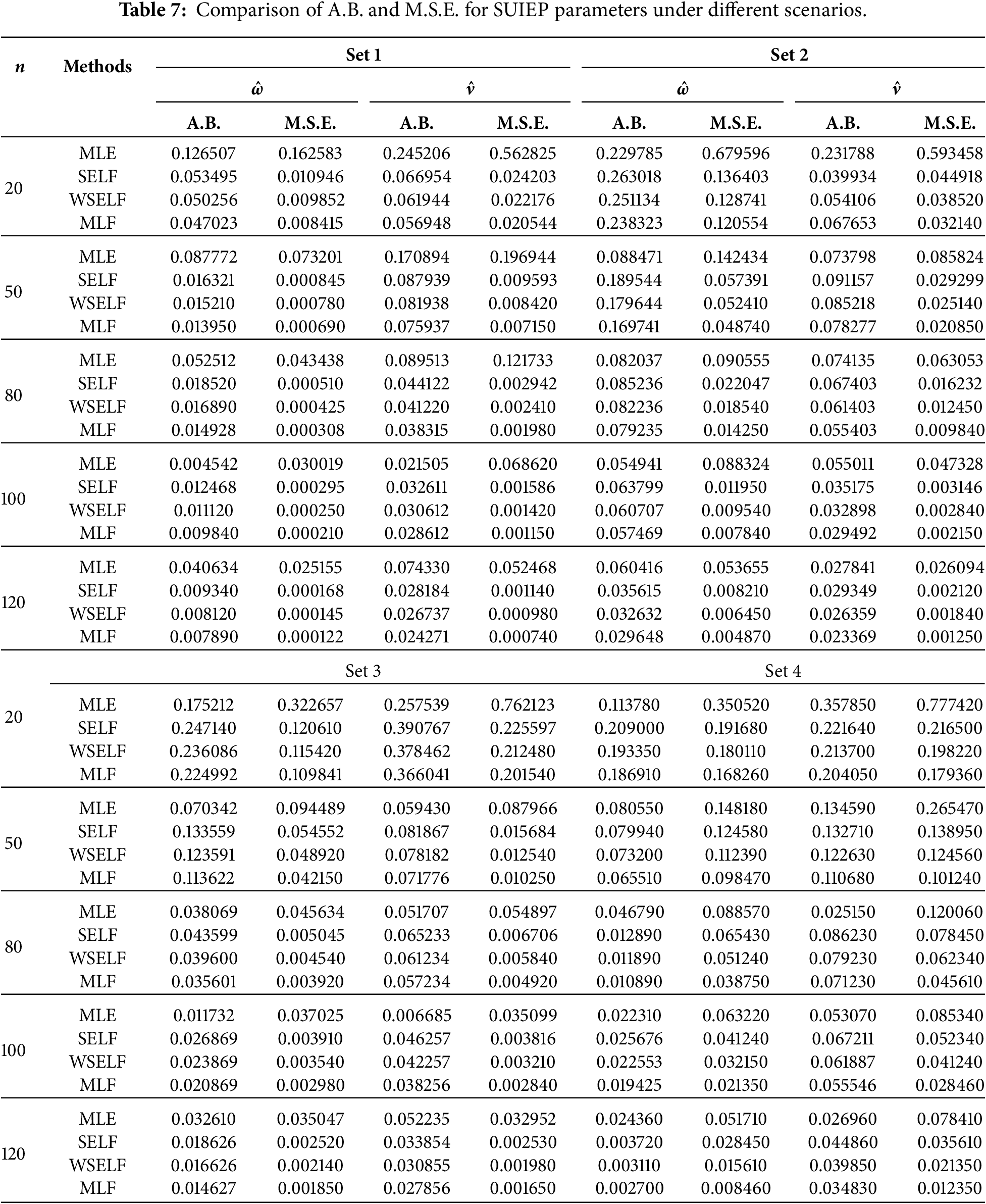
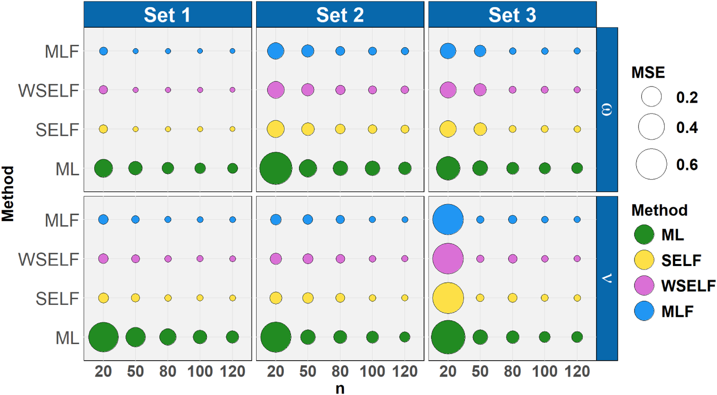
Figure 16: Comparative bubble plot of M.S.E. across different scenarios.

An analysis of how these estimates behave across various scenarios through the simulation reveals several critical points, which are outlined in the following summary:

1.   As visualized in Table 7 and Fig. 16, M.S.E. consistently decreases as the sample size increases, which confirms the asymptotic consistency of the estimators. However, A.B. does not exhibit a strictly monotonic decreasing trend and shows some fluctuations across different sample sizes, particularly within the Bayesian estimation framework.

2.   As illustrated in Fig. 16 and Table 7, the true parameter values influence estimation precision; larger parameter values generally tend to yield higher M.S.E. values in several scenarios, although this impact varies across different estimation methods and sample sizes.

3.   Table 7 shows that the M.S.E. performance between ω^ and ν^ depends on the specific parameter configuration; while ω^ yields lower M.S.E. values in certain scenarios (e.g., Set 1), ν^ produces lower M.S.E. values in others (e.g., Set 2), demonstrating that estimation precision varies across different parameter settings.

4.   Fig. 16 shows that Set 1 provided the most accurate estimates for ω^; however, it is not universally the most accurate for ν^, where performance varies depending on the specific sample size and estimation method.

5.   Table 7 indicates that the BE generally achieves better performance than the MLE by producing consistently lower M.S.E. values. However, the A.B. does not follow a strict pattern and varies depending on the sample size and the specific parameter set, with MLE occasionally yielding lower A.B. values in certain scenarios

6.   The results show that the BE under MLF outperformed WSELF, making it the most efficient choice in the majority of cases.

7.   While certain simulation results favored WSELF over SELF due to its lower M.S.E. values, both Bayesian loss functions demonstrated consistent accuracy as the sample size increased.

8.   Fig. 16 and Table 7 indicate that the MLF method generally achieves superior precision in terms of M.S.E. compared to the other evaluated methods, whereas performance regarding A.B. varies depending on the specific parameter configuration and sample size.

8  Conclusions

Construction of probability distributions capable of accommodating asymmetry is vital in carrying out the right analysis of asymmetric data. For this research work, the construction of a novel unit asymmetric probability distribution called the SUIEP distribution has been done. Various mathematical forms of some statistical properties have been derived. Graphical illustrations of such properties are presented, including the 3-D plots of mean, variance, skewness, and kurtosis; graphs of Lorenz and Bonferroni curves; a 3-D reliability graph of the SUIEP distribution; and graphs of entropies. Additionally, numerical values are obtained for some selected moments, as well as for the Rényi and Tsallis entropy measures. Parameter estimation has also been discussed using both classical and Bayesian approaches under symmetric and asymmetric loss functions. The complex Bayesian computation problem associated with the SUIEP distribution is easily solved via the use of the MCMC technique with independent gamma priors.

The simulation study confirms that larger sample sizes improve the estimation accuracy of the SUIEP distribution, with the Bayesian method under MLF providing the most precise results. The MCMC plots further verify these findings by showing stable parameter convergence, and our results also show that the estimate of ω is generally more accurate than the estimates of ν. These technical results are supported by the model’s excellent performance in real-world applications, such as analyzing COVID-19 mortality rates in Saudi Arabia and UAS detection proportions from the FAA records. In both cases, the SUIEP distribution proved to be a versatile and reliable tool, outperforming competing models. This demonstrates that the proposed distribution provides a promising statistical framework for analyzing both data sets, highlighting its potential applicability for modeling high-variability data in these critical sectors. One limitation of the current study is the fact that the analysis is done purely using the complete sample. In future research, it would be important to develop a framework where different types of censored data can be considered.

Acknowledgement: Princess Nourah bint Abdulrahman University Researchers Supporting Project number (PNURSP2026R734), Princess Nourah bint Abdulrahman University, Riyadh, Saudi Arabia.

Funding Statement: Princess Nourah bint Abdulrahman University Researchers Supporting Project number (PNURSP2026R734), Princess Nourah bint Abdulrahman University, Riyadh, Saudi Arabia.

Author Contributions: The author confirms contribution to the paper as follows: Rasha Alyousef: writing—original draft, software, formal analysis, conceptualization. Amal S. Hassan: writing—review & editing, writing—original draft, methodology, formal analysis, conceptualization. Omar A. Saudi: writing—original draft, software, formal analysis, visualization, conceptualization. Ohud A. Alqasem: writing—original draft, software, formal analysis, conceptualization. Mohammed Elgarhy: writing—original draft, software, formal analysis, conceptualization. All authors reviewed and approved the final version of the manuscript.

Availability of Data and Materials: The datasets analyzed during the current study are publicly available from their original sources, and the full extracted numerical values are included within Section 6 of this published article: (1) COVID-19 Mortality Rate Data: Derived from publicly available records as cited in [46], with the complete 36-day dataset provided in Section 6(a). (2) Air Defence Monitoring Data: Publicly available through the U.S. Federal Aviation Administration (FAA) at https://www.faa.gov/uas/resources/public_records/uas_sightings_report, with the complete 50-observation dataset provided in Section 6(b).

Ethics Approval: Not applicable.

Conflicts of Interest: The authors declare no conflicts of interest.

References

1. Mobarak MAE. An extension of three-parameter gamma-Weibull distribution: properties, estimation and applications. Egypt Stat J. 2026;70(1):111–36. [Google Scholar]

2. Souza L. New trigonometric classes of probabilistic distributions [dissertation]. Recife, Brazil: Universidade Federal Rural de Pernambuco; 2015. [Google Scholar]

3. Kumar D, Singh S, Singh SK. A new distribution using sine function: its application to bladder cancer patients data. J Stat Appl Probab. 2015;4(3):417–27. [Google Scholar]

4. Alkhairy I, Nagy M, Muse AH, Hussam E. The Arctan-X family of distributions: properties, simulation, and applications to actuarial sciences. Complexity. 2021;2021(1):4689010. doi:10.1155/2021/4689010. [Google Scholar] [CrossRef]

5. Chesneau C, Jamal F. The sine Kumaraswamy-G family of distributions. J Math Ext. 2020;15:1–33. doi:10.30495/JME.2021.1332. [Google Scholar] [CrossRef]

6. Kharazmi O, Saadatinik A. Hyperbolic cosine-F family of distributions with an application to exponential distribution. Gazi Univ J Sci. 2016;29(4):811–29. [Google Scholar]

7. Nanga S, Nasiru S, Dioggban J. Cosine Topp-Leone family of distributions: properties and regression. Res Math. 2023;10(1):2208935. doi:10.1080/27684830.2023.2208935. [Google Scholar] [CrossRef]

8. Alshanbari HM, Ahmad Z, Al-Mofleh H, Ampadu CB, Khosa SK. A new probabilistic approach: estimation and Monte Carlo simulation with applications to time-to-event data. Mathematics. 2023;11(7):1583. doi:10.3390/math11071583. [Google Scholar] [CrossRef]

9. Osi A, Abdalla G, Sawaran Singh NS, Suleiman A. Advancing lifetime data modeling via the Marshall-Olkin cosine Topp-Leone distribution family. Comput J Math Stat Sci. 2025;4(2):476–99. doi:10.21608/cjmss.2025.374786.1155. [Google Scholar] [CrossRef]

10. Alghamdi AS, ALoufi SF, Baharith LA. The sine alpha power-G family of distributions: characterizations, regression modeling, and applications. Symmetry. 2025;17(3):468. doi:10.3390/sym17030468. [Google Scholar] [CrossRef]

11. David IJ, Stephen M, Thomas EJ. Reliability analysis with new sine inverse Rayleigh distribution. J Reliab Stat Stud. 2023;16(2):255–68. doi:10.13052/jrss0974-8024.1623. [Google Scholar] [CrossRef]

12. Almarashi AM. Sine power Lindley distribution with applications. Intell Autom Soft Comput. 2022;31(1):373–86. doi:10.32604/iasc.2022.018043. [Google Scholar] [CrossRef]

13. Aldahlan MA. Sine Fréchet model: modeling of COVID-19 death cases in Kingdom of Saudi Arabia. Math Probl Eng. 2022;2022(3):2039076. doi:10.1155/2022/2039076. [Google Scholar] [CrossRef]

14. Nedjar MS, Zeghdoudi HM, Alqifari HN. Statistical properties of the sine new X-Lindley distribution: fuzzy reliability analysis and applications. AIMS Math. 2025;11(4):11924–47. [Google Scholar]

15. Fayomi A, Algarni A, Almarashi AM. Sine inverse lomax generated family of distributions with applications. Math Probl Eng. 2021;1267420:1–11. doi:10.1155/2021/1267420. [Google Scholar] [CrossRef]

16. Shrahili M, Elbatal I, Elgarhy M. Sine half-logistic inverse Rayleigh distribution: properties, estimation, and applications in biomedical data. J Math. 2021;2021(3):1–10. doi:10.1155/2021/4220479. [Google Scholar] [CrossRef]

17. Nagarjuna VBV, Vardhan RV, Chesneau C. On the accuracy of the sine power lomax model for data fitting. Modeling. 2021;2(1):78–104. doi:10.3390/modelling2010005. [Google Scholar] [CrossRef]

18. Hassan A, Saudi O, Nagy H. A novel two-parameter sine model: Bayesian and non-Bayesian analysis with application. Gazi Univ J Sci. 2026. doi:10.35378/gujs.1583397. [Google Scholar] [CrossRef]

19. Tomy L, Chesneau C. The sine modified Lindley distribution. Math Comput Appl. 2021;26(4):81. doi:10.3390/mca26040081. [Google Scholar] [CrossRef]

20. Hassan AS, Ali EIA, Hamdani H, Gemeay AM, Shawki AW, Elgarhy M. A comparative study of estimation methods for the new sine Topp-Leone Fréchet distribution. Sci Afr. 2026;31(4):e03142. doi:10.1016/j.sciaf.2025.e03142. [Google Scholar] [CrossRef]

21. Adepoju AA, Bello AO, Isa AM, Adesupo A, Olumoh JS. Statistical inference on sine-exponential distribution parameter. J Comput Innov Anal. 2024;3(2):129–45. doi:10.32890/jcia2024.3.2.6. [Google Scholar] [CrossRef]

22. Genç M, Özbilen Ö. Sine unit exponentiated half-logistic distribution: theory, estimation, and applications in reliability modeling. Mathematics. 2025;13(11):1871. doi:10.3390/math13111871. [Google Scholar] [CrossRef]

23. Bashiru SO, Moakofi T. Sine type II Topp-Leone Gompertz distribution with applications. Ann Commun Math. 2025;8(2):275–92. doi:10.62072/acm.2025.080210. [Google Scholar] [CrossRef]

24. Bleed S, Abdelali A. Transmuted arcsine distribution properties and application. Int J Res. 2018;10:1–11. doi:10.29121/granthaalayah.v6.i10.2018.1159. [Google Scholar] [CrossRef]

25. Shah Z, Ahmad Z, Almaspoor Z, Khan F, Onyekwere CK, Rao GS. A novel flexible logarithmic cosine-G family of distributions with applications to event time data. Mod J Stat. 2026;2(2):81–102. doi:10.64389/mjs.2026.02283. [Google Scholar] [CrossRef]

26. Khamees WA, Hassan AS, El-Kholy AK, Helmy BA. A novel flexible model: the sine topp leone length-biased truncated lomax distribution. Open J Math Sci. 2026;10:556–77. doi:10.30538/oms2026.0305. [Google Scholar] [CrossRef]

27. Mustpha MH, Jakperik D, Nasiru S. Tangent exponentiated odd log-logistic Weibull quantile regression with applications to complete and censored data. Egypt Stat J. 2025;69(1):173–205. doi:10.21608/esju.2025.359062.1070. [Google Scholar] [CrossRef]

28. Amer YM, Abdel Hady DH, Shalabi RM. A novel family of continuous-discrete bivariate distributions. Comput J Math Stat Sci. 2026;5(1):415–37. doi:10.21608/cjmss.2025.405765.1233. [Google Scholar] [CrossRef]

29. Christophe C. Theory on a new bivariate trigonometric Gaussian distribution. Innov Stat Probab. 2025;1(2):1–17. doi:10.64389/isp.2025.01223. [Google Scholar] [CrossRef]

30. Hassan AS, Alomani G, Al-Omari AI, Hassan MM. Modeling engineering and medical lifetime data using a flexible extension of the XShanker distribution under censoring. Sci Rep. 2026;16(1):24355. doi:10.1038/s41598-026-52861-5. [Google Scholar] [CrossRef]

31. Hassan AS, Abdalla GSS, Faal A, Saudi OA. Novel unit distribution for enhanced modeling capabilities: healthcare and geological applications. Eng Rep. 2025;7(7):e70277. doi:10.1002/eng2.70277. [Google Scholar] [CrossRef]

32. Gradshteyn IS, Ryzhik IM. Table of integrals, series, and products. San Diego, CA, USA: Academic Press; 2014. [Google Scholar]

33. Rényi A. On measures of entropy and information. In: Proceedings of the Fourth Berkeley Symposium on Mathematical Statistics and Probability; 1960 Jul 20–30; Berkeley, CA, USA. p. 547–61. [Google Scholar]

34. Tsallis C. Possible generalization of Boltzmann-Gibbs statistics. J Stat Phys. 1988;52(1–2):479–87. doi:10.1007/BF01016429. [Google Scholar] [CrossRef]

35. Tummala VR, Sathe PT. Minimum expected loss estimators of reliability and parameters of certain lifetime distributions. IEEE Trans Reliab. 1978;27(4):283–5. doi:10.1109/tr.1978.5220373. [Google Scholar] [CrossRef]

36. Tinochai K, Jampachaisri K. The performance of empirical Bayes based on weighted squared error loss and K-loss functions in skip lot sampling plan with resampling. Eng Lett. 2022;30(2):379. [Google Scholar]

37. Ali S, Aslam M, Kazmi SMA. A study of the effect of the loss function on Bayes estimate, posterior risk and hazard function for Lindley distribution. Appl Math Model. 2013;37(8):6068–78. doi:10.1016/j.apm.2012.12.008. [Google Scholar] [CrossRef]

38. Dey S, Singh S, Tripathi YM, Asgharzadeh A. Estimation and prediction for a progressively censored generalized inverted exponential distribution. Stat Methodol. 2016;32(4):185–202. doi:10.1016/j.stamet.2016.05.007. [Google Scholar] [CrossRef]

39. Metropolis N, Rosenbluth AW, Rosenbluth MN, Teller AH, Teller E. Equation of state calculations by fast computing machines. J Chem Phys. 1953;21(6):1087–92. doi:10.1063/1.1699114. [Google Scholar] [CrossRef]

40. Mazucheli J, Menezes AFB, Ghitany ME. The unit-Weibull distribution and associated inference. J Appl Probab Stat. 2018;13(2):1–22. [Google Scholar]

41. Mazucheli J, Menezes AF, Dey S. Unit-Gompertz distribution with applications. Statistica. 2019;79(1):25–43. [Google Scholar]

42. Afuecheta E, Okorie IE, Jallow H, Nadarajah S. A review of unit continuous probability distributions. AIMS Math. 2025;10(11):25939–6057. doi:10.3934/math.20251146. [Google Scholar] [CrossRef]

43. Ribeiro-Reis LD. Truncated exponentiated-exponential distribution: a distribution for unit interval. J Stat Manag Syst. 2022;25(8):2061–72. [Google Scholar]

44. Hassan A, Khalil A, Nagy H. Versatile extension of the unit Gompertz: efficient estimation and application. Gazi Univ J Sci. 2025;38(3):1540–64. doi:10.35378/gujs.1541941. [Google Scholar] [CrossRef]

45. Hassan AS, Metwally DA, Elgarhy M, Semary HE, Faal A, Mohamed RE. Sine power unit inverse Lindley model: Bayesian analysis and practical application. Eng Rep. 2025;7:e70242. [Google Scholar]

46. Alotaibi N, Al-Moisheer AS, Hassan AS, Elbatal I, Alyami SA, Almetwally EM. Epidemiological modeling of COVID-19 data with Advanced statistical inference based on Type-II progressive censoring. Heliyon. 2024;10(18):e36774. [Google Scholar]