
 Login
Login Register
 Submit a Paper
 Propose a Special lssue
 Open Access
ARTICLE
Multi-Surface Knee Joint Kinematics Estimation Using Hybrid Stacked Long Short-Term Memory-Multilayer Perceptron Network
1 Department of Mechanical Engineering and Product Design Engineering, Swinburne University of Technology, Melbourne, Australia
2 Department of Engineering Technologies, Swinburne University of Technology, Melbourne, Australia
3 Department of Allied Health, Swinburne University of Technology, Melbourne, Australia
4 Department of Medicine (Royal Melbourne Hospital), The University of Melbourne, Melbourne, Australia
5 Department of Biomechanics, Victoria University, Melbourne, Australia
* Corresponding Authors: Kwong Ming Tse. Email: ,
Computer Modeling in Engineering & Sciences 2026, 148(3), 15 https://doi.org/10.32604/cmes.2026.086130
Received 25 May 2026; Accepted 25 August 2026; Issue published 28 September 2026
 View Full Text
 Download PDF
Abstract
The estimation of lower limb joint kinematics has great potential to be used for different applications, for instance, gait analysis, diagnosis of any joint injury, diagnosis of any other lower limb injury, prosthesis control, etc. The natural and controlled interaction between human and lower limb prosthesis is very important. Hybrid Stacked Long Short-Term Memory-Multilayer Perceptron (HS-LSTM-MLP) network is hypothesized to estimate knee joint angle individually over five different surfaces: level ground, ramp ascent, ramp descent, stair ascent, and stair descent. The spatial and temporal information extracted from reflective markers is used as input features, and the calculated knee joint angles are used as the target variable. The standard performance metrics for such regression tasks, including coefficient of determination (R2), mean squared error (MSE), and root mean square error (RMSE), are employed here for proposed model evaluation. The proposed HS-LSTM-MLP model is compared with the state-of-the-art Bidirectional Long Short-Term Memory (BiLSTM), Long Short-Term Memory (LSTM), and Multilayer Perceptron (MLP) neural networks to evaluate its efficiency for knee joint angle estimation. The HS-LSTM-MLP model outperforms BiLSTM, LSTM, and MLP with R2 (above 0.9513, 0.9435, 0.9340, and 0.9111, respectively) and RMSE (below 4.6395°, 5.1667°, 6.2338°, and 7.6487°, respectively). The estimation results are simulated in MATLAB for a proof-of-concept for potential application in transfemoral powered prostheses. The proposed model HS-LSTM-MLP exhibits significant potential for precise and reliable knee joint angle estimation and to enable amputees in the future to walk over different surfaces with more efficient knee joint control and greater stability.Keywords
Supplementary Material
Supplementary Material FileLower-limb prostheses have evolved substantially, from passive and semi-active devices to active or powered systems designed to better support the mobility demands of people with limb loss [1]. Among these, powered prostheses represent the current state-of-the-art because they can assist movement across a range of daily tasks. However, their effectiveness depends on how accurately and how quickly they can interpret the user’s intended motion and generate an appropriate mechanical response [2]. Reliable estimation of gait and joint kinematics is therefore a key prerequisite for intuitive, stable, and safe ambulation. Beyond prosthetic control, joint-level kinematic estimation is also valuable for the assessment, diagnosis, and monitoring of gait disorders [3].
Within lower-limb locomotion, the knee joint is of particular importance because it contributes to stance stability, shock absorption, swing clearance, and adaptation to demanding tasks such as ramp and stair negotiation [4–6]. This is especially relevant in transfemoral amputation, where the biological knee is absent, and its function must be replaced by the prosthetic system. As a result, accurate estimation of knee joint kinematics is central to improving the control of powered transfemoral prostheses and supporting functional mobility across everyday ambulation tasks [7,8].
A wide range of machine-learning approaches have been explored to estimate knee kinematics. Many of the strongest-performing models have used surface electromyography (sEMG) as input since muscle activation precedes observable movement and can therefore support anticipatory control. For instance, Li et al. [9] estimated continuous knee joint kinematics from sEMG using multiple-kernel relevance vector regression (MKRVR) and reported good predictive performance, outperforming a least-squares support vector regression comparator. Another latest research demonstrated the feasibility of deep learning by proposing a one-dimensional U-Net architecture to estimate knee joint angles directly from sEMG signals in pediatric gait, achieving RMSE values of 4.1° [10]. However, it is observed that lower limb muscles provide sEMG signals 20 to 200 ms ahead of motion [11,12]. Previously, it was investigated that this factor can lead to an error of around 4° to estimate forthcoming knee joint angle during walking [2]. Together, these studies highlight that timing is crucial in motion-intention recognition, particularly where low-latency or slightly anticipatory predictions are needed to accommodate processing and actuator delays.
Despite all this, sEMG-based approaches also increase system complexity and burden. They require additional sensors, careful skin preparation and placement, and can be affected by noise, sweat, and signal variability [13–15]. These limitations have motivated interest in whether knee kinematics can be estimated accurately by kinematic inputs alone, without relying on sEMG. Supporting this possibility, Bian et al. [2] demonstrated that short-horizon (10 ms) prediction of lower-limb sagittal-plane joint angles could be achieved using kinematic information obtained from optical motion capture and IMU sensors. Their stacked LSTM architecture outperformed both a feedforward MLP and the specific hybrid LSTM-MLP architecture investigated in their study. However, their work focused on short-horizon gait-intention prediction using multimodal kinematic inputs, whereas the present study proposes a different HS-LSTM-MLP architecture for multi-surface continuous knee joint kinematics estimation using only reflective marker trajectories. This suggests that kinematics-only approaches may provide a more practical alternative when sEMG is unavailable or impractical.
Recent research has also increasingly focused on minimally instrumented wearable solutions, most notably inertial measurement unit (IMU)-based systems for joint kinematics estimation. In a clinical population, Tan et al. [16] used a Bidirectional LSTM model to predict sagittal-plane knee flexion from IMU data in people with knee osteoarthritis during walking, stair negotiation, and chair transfers, supporting the feasibility of IMU-based knee kinematic estimation across functional tasks. More recently, an LSTM-based framework was developed to estimate contralateral knee joint angles from four IMUs for transfemoral prosthesis control, achieving real-time RMSE values of 2.48°–2.78° and correlation coefficients of 0.9937–0.9991 in able-bodied participants, thereby demonstrating the potential of recurrent neural networks for accurate IMU-based knee kinematics estimation [17]. Ackland et al. [18] further showed that hip, knee, and ankle joint kinematics could be predicted from IMU data alone using a generative adversarial network, with sagittal-plane errors below 4° during walking and improved accuracy when more sensors were used. Collectively, these studies indicate that wearable sensors can provide useful estimates of lower-limb kinematics, but they also show that performance depends on sensor number, placement, calibration, and modelling strategy.
This dependence on implementation details is reinforced by validation studies focused specifically on knee kinematics. Cornish et al. [19] reported that two IMUs could provide very good to excellent agreement with optical motion capture for sagittal-plane knee joint angle during daily living activities following total knee arthroplasty, although performance was less robust outside the sagittal plane. Wang et al. [20] showed that sensor-to-bone calibration is critical for obtaining clinically meaningful knee-angle estimates during gait from IMU data, while Weber et al. [7] demonstrated that fixation method substantially influences IMU-based knee kinematics, with harness-mounted sensors outperforming skin-mounted sensors after reference-frame alignment. Thus, although IMUs are portable and attractive for wearable applications, their accuracy remains sensitive to attachment, alignment, and calibration procedures.
Taken together, the literature suggests two important points. First, accurate and temporally meaningful prediction of knee kinematics is feasible using machine-learning approaches. Second, there remains a trade-off between practicality and reference-quality measurement: wearable solutions reduce instrumentation burden but may be affected by sensor placement, fixation, and calibration, whereas optical motion capture remains the reference standard for deriving high-quality kinematic data. This creates a need to explore alternative input representations and modelling strategies that may ultimately support lower-burden prediction of knee joint kinematics while retaining high accuracy.
The present study aims to estimate knee joint kinematics relevant to transfemoral prosthesis use across five locomotor conditions: level ground, ramp ascent, ramp descent, stair ascent, and stair descent. Rather than introducing an immediately deployable low-cost sensing setup, this study used motion-capture-derived kinematic signals as a reference-quality input source to establish and evaluate a novel Hybrid Stacked Long Short-Term Memory-Multilayer Perceptron (HS-LSTM-MLP) model. In this way, the study provides proof-of-concept for temporal knee-angle prediction across functionally relevant ambulation tasks, with the longer-term goal of informing future lower-burden implementations for powered prosthetic control.
A total of 20 healthy participants (gender: 40% female, 60% male; age 31.8 ± 6.2 years; body mass 67.7 ± 9.2 kg; height 1.68 ± 0.09 m; BMI 23.8 ± 1.7 kg/m2) were recruited for data collection. All participants reported no history of lower-limb injury, physical disability, or neurological disorder. Participants’ data from both legs were recorded using a 12-camera Qualisys 3D Motion Capture System (USA). A treadmill (LANDICE—ProForm Carbon Pro 2000) was used to collect data during level-ground walking. For ramp locomotion, a 5 m ramp with a 7° incline was used for both ramp ascend and descend trials, while a four-step staircase was employed to record stair ascend and descend. The sampling frequency of the Qualisys Motion Capture System was set to 100 Hz. In total, 19 reflective markers were placed on the lower limb to track knee joint angular kinematics [11]. The names and anatomical locations of the markers are illustrated in Fig. 1. This research involving humans was approved by Swinburne University of Technology Human Research Ethics Committee (SUHREC), Australia (Reference no.: 20246933-17851 and date of approval: 6 March 2024). The research was conducted in accordance with the institutional requirements. The participants provided their written informed consent to participate in this research. Written informed consent was obtained from the individuals for the publication of any images or data included in this article.
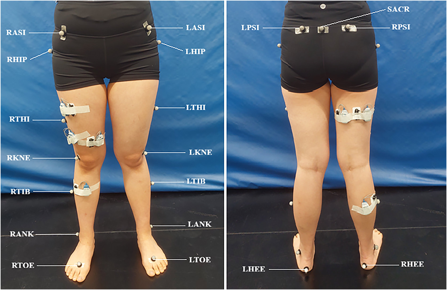
Figure 1: Illustration of the 19 markers and their anatomical positions on a participant’s lower limbs for tracking knee joint angular kinematics. SACR = sacrum, RPSI = right posterior superior iliac, LPSI = left posterior superior iliac, RASI = right anterior superior iliac, LASI = left anterior superior iliac, RHIP = right lateral hip, LHIP = left lateral hip, RTHI = right lateral thigh, LTHI = left lateral thigh, RKNE = right lateral knee, LKNE = left lateral knee, RTIB = right lateral tibia, LTIB = left lateral tibia, RANK = right lateral ankle, LANK = left lateral ankle, RTOE = right toe, LTOE = left toe, RHEE = right heel, LHEE = left heel.
Depending on participants’ availability, data collection was conducted across one or two sessions, separated by 14–20 days (mean ≈ 15 days), a duration unlikely to influence marker-based measurements. Some previous studies have demonstrated that marker-based motion capture systems provide good test–retest reliability for lower-limb kinematics across different testing sessions, with small variations [21,22]. Reflective markers were attached at predefined anatomical locations, and kinematic data were recorded using the Qualisys Track Manager (QTM) system. Participants first walked barefoot on the treadmill at a self-selected comfortable speed of 1.4 m/s for level-ground walking trials. Prior to data collection, participants were provided with a familiarization period to practice treadmill walking, and the speed was selected based on their comfort and ability to maintain a stable and natural gait pattern throughout the trial. A 5-min rest period was provided before completing the ramp and stair trials.
Similarly, ramp and stair locomotion speeds were determined by participants’ self-selected comfortable pace to ensure safe and natural movement execution. For ramp trials, participants required approximately 8 s to complete either ascent or descent. Continuous walking was performed for five trials per session, resulting in 40 s of data for each ramp condition. Three sessions were conducted to obtain 120 s of data for each ramp surface, with a 5-min rest period between sessions. For stair trials, each ascent or descent required approximately 6 s at a natural walking speed. Participants completed five trials per session, generating 30 s of data per condition. To obtain 120 s of data for each stair condition, four sessions were conducted, with a 5-min rest period after every session. Prior to ramp and stair trials, participants performed practice runs to familiarise themselves with the setup and maintain a consistent walking pace (approximately 8 s for ramp ascent and descent, and 6 s for stair ascent and descent). The laboratory setup, schematic representation of the experimental setup, and examples of participants walking on different surfaces are shown in Figs. 2–4. Marker trajectory data used for kinematic prediction were recorded using the QTM system.
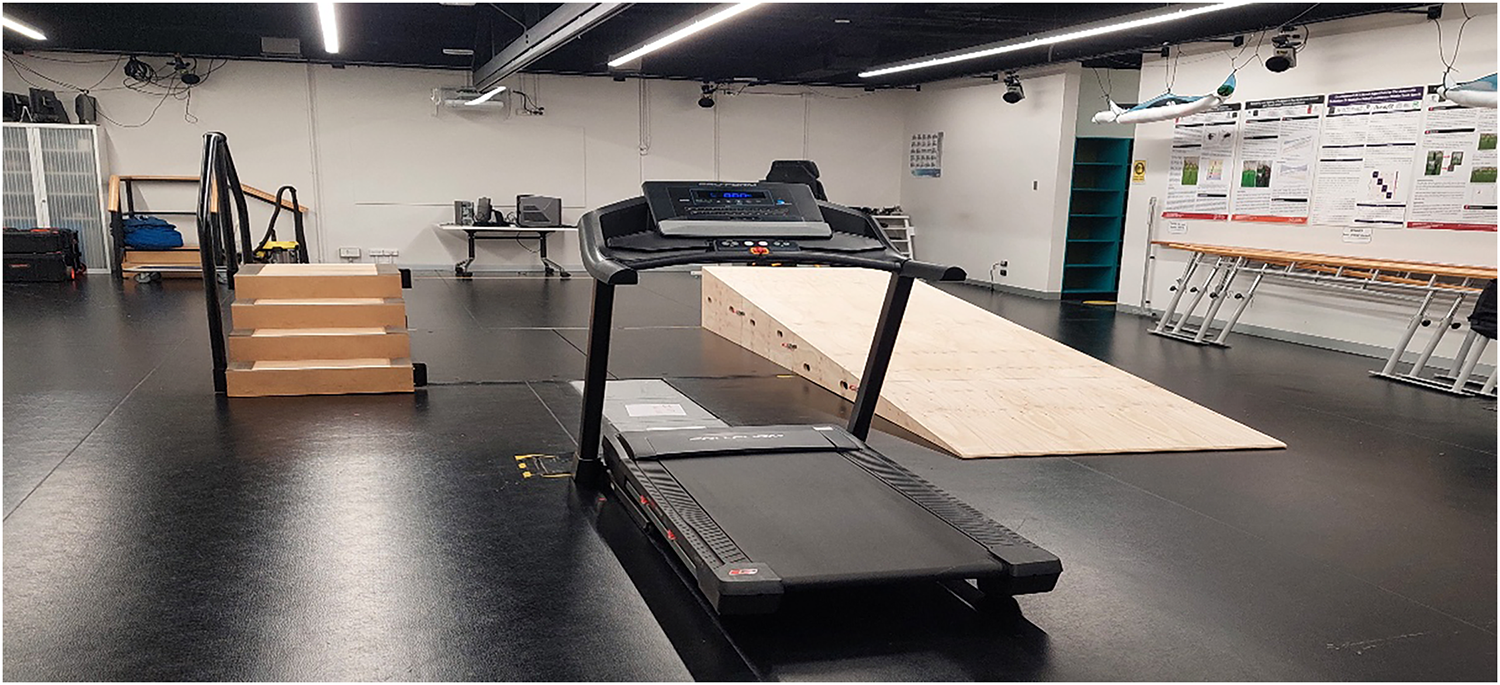
Figure 2: Experimental setup for treadmill, ramp and staircase in lab.
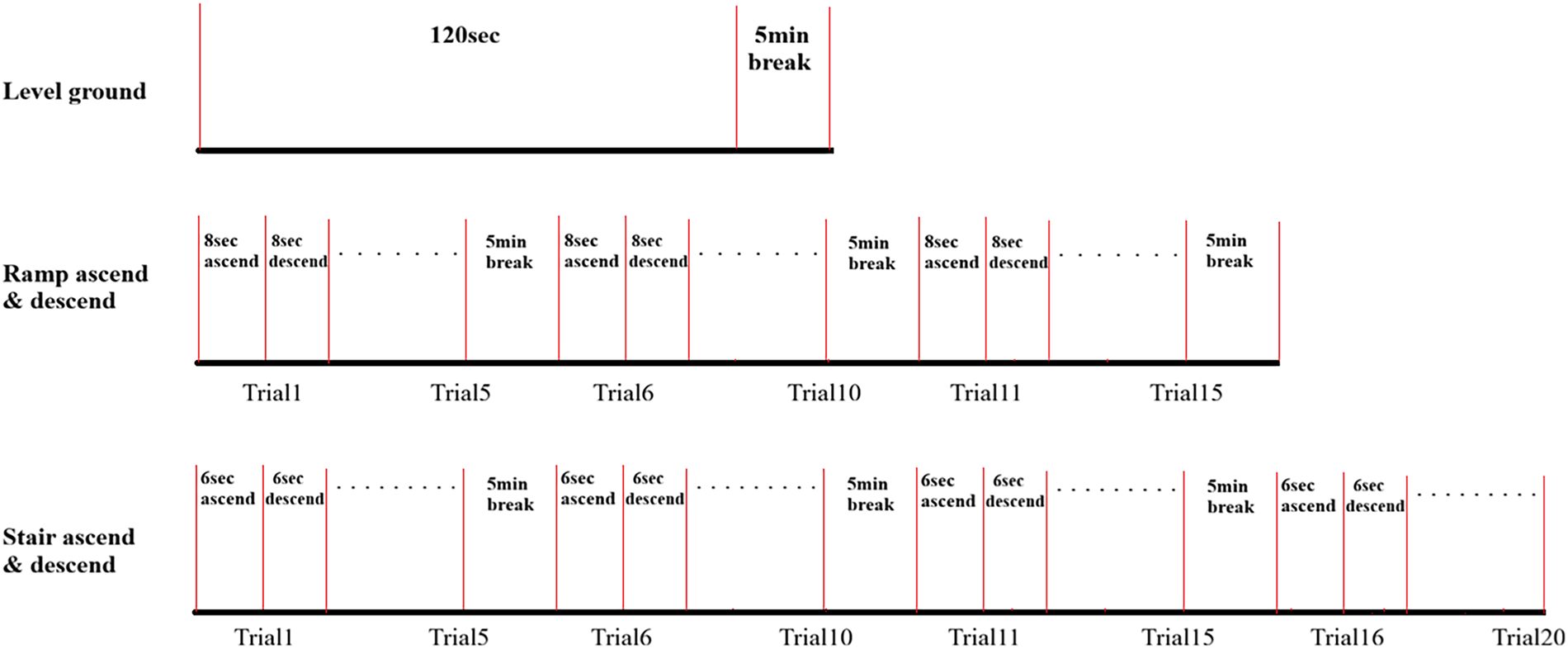
Figure 3: Schematic diagram of experimental setup for data collection.
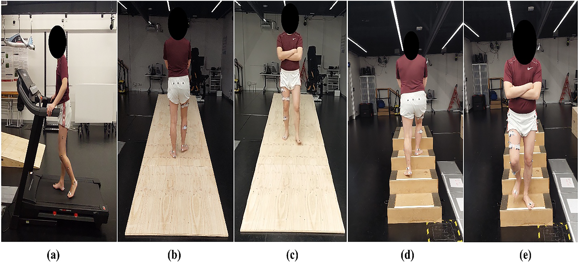
Figure 4: Participant walking on different surfaces: (a) level ground, (b) ramp ascent, (c) ramp descent, (d) stair ascent, and (e) stair descent.
2.2 Data Processing and Feature Extraction
Marker data were first interpolated and labelled in Qualisys prior to being exported to MATLAB for further analysis. Each raw marker spatial coordinates (x, y, z) were retained for analysis and was pre-processed using a fourth-order Butterworth low-pass filter with a cutoff frequency of 6 Hz to remove inherent noise [23]. The lower limb is normally represented by the kinematics and dynamics of hip, knee, and ankle joints [18,24]. During walking, ramp negotiation, and stair negotiation, the dominant movements of the lower limbs, particularly hip flexion/extension, knee flexion/extension and ankle dorsiflexion/plantarflexion, occurs primarily in the sagittal plane [25]. Accordingly, the marker trajectories were projected onto a sagittal coordinate frame to focus the analysis on flexion–extension kinematics and exclude the mediolateral component from subsequent knee-angle estimation [26]. Marker trajectories from both the left and right lower limbs were processed to construct the input dataset. However, statistical analyses and the performance summaries were calculated across the 20 participants, and the left and right limbs were not treated as independent participants.
In modelling knee-joint flexion or extension from marker data, the choice of input features is crucial. Rather than relying purely on raw marker positions, biomechanically meaningful and temporal-aware features were derived that capture thigh-shank geometry and dynamics. These features facilitate machine-learning models (MLP, LSTM, BiLSTM, and HS-LSTM-MLP) that generalize across different surfaces (level walking, ramp ascent, ramp descent, stair ascent, and stair descent) and subjects.
2.2.1 Thigh and Shank Segment Vectors
Segment vectors for thigh and shank were employed in features [27,28]:
where H, K, and A are the 3D hip, knee, and ankle marker coordinates (sagittal plane). From these vectors, segment lengths in the sagittal plane were derived. These lengths capture anthropometric scaling and help normalize for subject leg-length differences [29,30].
Next, segment vectors and segment lengths help provide unit vectors, which remove magnitude dependence and provide pure orientation information.
Knee joint kinematics are inherently dynamic, and segment velocities and angular velocities provide important information about the rate and direction of limb motion [31,32]. These temporal features help capture gait phase progression and support smooth transition modelling, thereby improving prediction stability. Incorporating derivative-based motion information allows machine-learning models to distinguish phases where flexion or extension accelerates or decelerates, enhancing temporal sensitivity without explicitly requiring past angle values. Segment velocities were computed using Eqs. (7) and (8) [33,34].
Unit vector rates (angular-change proxy) were calculated by following Eqs. (9) and (10).
where d_vt, d_vs are first derivatives of thigh and shank vectors (velocity), i.e., segment velocities, and d_uT, d_uS are first derivatives of unit vectors (angular velocity proxies), i.e., angular-rate proxies.
Knee flexion-extension during level walking, ramp, and stair ambulation is mainly confined to low-frequency components below about 5–6 Hz, while higher frequencies typically reflect noise or soft tissue artefacts [35]. To preserve physiologically relevant motion, a fourth-order low-pass Butterworth filter was applied to both input features and target angles [16].
Knee joint angle was calculated to be used as the target variable in machine learning (ML) training models. The knee joint angle was defined as the sagittal-plane angle between the thigh segment vector (formed from knee to hip markers) and the shank segment vector (formed from knee to ankle markers). To calculate the knee joint angles formed by three markers (hip, knee, and ankle), vectors between pairs of markers were required to be computed, and then the angle between these vectors was calculated using the dot product [36–38].
For these three markers; P1, P2 and P3:
Vector v1 = P2 − P1
Vector v2 = P3 − P2
The angle θ between vectors v1 and v2 is calculated by:
where:
a1·a2 = dot product of two vectors
||a1|| and ||a2|| = magnitudes of vectors
Knee flexion was represented as the positive angular direction. Since joint angle magnitudes can vary depending on coordinate system conventions, filtering approaches, marker definitions, and biomechanical modelling approaches, comparisons with normative gait datasets require consistent angle definitions and processing methodologies.
2.3 Long Short-Term Memory (LSTM)
LSTM is a specifically designed recurrent neural network (RNN) that basically serves to resolve the vanishing gradient issue occurring during long sequence training [39]. This capability makes LSTM a preferred choice for tasks involving long-term dependencies [40]. The key feature of LSTM architecture is the cell state or memory cell, which provides paths for the gradient to flow, hence resolving the vanishing gradient problem [41]. The LSTM architecture incorporates three gating mechanisms that regulate the internal cell state: the forget gate (ft), input gate (it), and output gate (ot). The forget gate determines which information from the previous cell state should be retained or discarded. The input gate governs the incorporation of new information into the memory cell, while the output gate controls the portion of the internal state that is propagated to the subsequent time step. Together, these gates enable selective information flow, allowing the network to preserve meaningful long-term dependencies [42]. The sigmoid activation function constrains real-valued inputs to the interval (0, 1), whereas the hyperbolic tangent (tanh) function maps inputs to the range (−1, 1).
Below, the mathematical form of the LSTM cell is given in Eqs. (12)–(16).
where xt denotes the input vector at time step t, and ht−1 represents the hidden state (network output) from the preceding time step. The symbol
An activation function is a mathematical operation that determines the output of a neuron based on its weighted inputs [43]. It plays a critical role in neural networks by introducing nonlinearity, allowing the model to capture complex relationships between input variables and predicted outputs [44]. Commonly used activation functions in ML and deep learning include the sigmoid, hyperbolic tangent (tanh), and Rectified Linear Unit (ReLU). The sigmoid function compresses real-valued inputs into the range (0, 1), making it particularly suitable for probabilistic interpretations and binary classification tasks. The tanh function generates outputs between (−1, 1) and is zero-centred, which facilitates modelling both positive and negative feature influences. Due to its smooth nonlinear characteristics, tanh is frequently implemented in recurrent neural networks [45]. ReLU is widely adopted in contemporary deep-learning architectures because of its computational efficiency and its ability to alleviate gradient attenuation during backpropagation [46]. It outputs zero for negative inputs and retains positive values unchanged, promoting faster convergence, although it can sometimes result in inactive (“dead”) neurons. The selection of an activation function in the output layer ultimately depends on the specific learning objective and task requirements.
2.3.2 Choice of LSTM Structural Parameters
In this research, a stacked LSTM network was adapted with two layers to train the knee joint kinematics estimation model. It comprises an input layer, two hidden layers, and an output layer. The input layer contained fourteen nodes that were raw sagittal-plane marker trajectories of the hip, knee, and ankle, thigh and shank segment velocities, and thigh and shank unit-vector rates. There were 256 hidden units in the first layer and 128 hidden units in the second layer. The target vector was the knee joint angle sequence calculated from marker data. The Adam optimization algorithm with 100 rounds of training in a mini-batch size (1024) was used to minimize the loss function, and the learning rate was set to 0.02. The dropout method was used as a regularization method, and the dropout rate was set to 0.3. Then, an additional fully connected time-distributed layer with a rectified linear unit (ReLU) activation function was used for non-linearity. At the end, a separate fully connected time-distributed output layer with a regression layer was used to return the estimated joint angle.
LSTM networks are effective at learning temporal dependencies in sequential data and, in this study, can model dynamic variations in joint kinematics across different walking surfaces. However, their sequential processing leads to computational inefficiency for long input sequences. Although LSTMs mitigate the vanishing-gradient problem of traditional RNNs, this issue may still arise in deeper or stacked architectures. In addition, LSTMs incur high computational and memory costs, resulting in slow training for large datasets. They may also overfit and remain sensitive to noisy biomechanical signals, which can limit generalisation across varying surfaces and participants.
2.4 Bidirectional Long Short-Term Memory (BiLSTM)
Bidirectional Long Short-Term Memory (BiLSTM) is an extension of the standard LSTM architecture that processes sequential data in both forward and backward directions [16]. Unlike conventional neural networks that analyze sequences only once in chronological order, BiLSTM employs two parallel LSTM layers: one capturing past-to-future dependencies and the other capturing future-to-past information, in the form of feedback [47]. By integrating context from both temporal directions, BiLSTM can learn richer sequence representations and often achieves improved predictive performance compared with unidirectional LSTM models [48]. Each BiLSTM layer therefore consists of two LSTM units operating in forward (LSTM1) and backward directions
Then, using LSTM2, the input sequence is processed in the reverse direction, and the backward hidden states (hb) are calculated as follows:
The ultimate hidden state (hi) is obtained by merging the forward and backward hidden states as follows:
2.4.2 Choice of BiLSTM Structural Parameters
In this research, a stacked Bidirectional Long Short-Term Memory (BiLSTM) network was employed to estimate knee joint angles from markers and their features. The same input features and target vector were employed, as in LSTM. Two BiLSTM layers were arranged sequentially to model temporal dependencies in the input sequences. The first BiLSTM layer contained 384 hidden units, followed by a second layer with 256 hidden units, enabling hierarchical feature extraction from the sequential marker data. Model training was performed using the Adam optimisation algorithm for 100 epochs with a mini-batch size of 1024, and the initial learning rate was set to 0.01. Dropout regularisation with a rate of 0.3 was incorporated to reduce overfitting and improve generalisation. Following the recurrent layers, an additional fully connected time-distributed layer with a ReLU activation function was included to introduce a nonlinear transformation of the learned representations. Finally, a time-distributed fully connected output layer combined with a regression layer was used to produce the estimated knee joint angle sequence.
The bidirectional structure allows the model to utilise both past and future temporal context, providing improved sequence representation compared with a standard LSTM. However, this advantage comes at the cost of increased computational complexity, larger parameter count, and higher memory requirements, which may increase overfitting risk and limit real-time deployment in resource-constrained applications such as prosthetic devices.
2.5 Multilayer Perceptron (MLP)
Multilayer Perceptron (MLP) is a subcategory of feedforward neural network (FNN) composed of multiple layers of interconnected computational units, commonly referred to as neurons or perceptrons [38]. These neurons are linked through weighted connections that enable information to propagate through the network. A typical Multilayer Perceptron (MLP) architecture includes an input layer that accepts the feature variables, one or more hidden layers that apply nonlinear mappings to extract underlying patterns, and an output layer that produces the final predicted outcome [50]. Through this layered structure, MLP can approximate complex nonlinear relationships and, under suitable conditions, can approximate any continuous function. MLPs are typically trained using supervised learning, where the model learns a mapping between input features and corresponding target outputs [51]. During the training phase, data propagate forward through the network, generating predictions according to the existing weights and bias parameters. The discrepancy between the predicted values and the true targets is evaluated using a defined loss function. This error is then transmitted backward across the layers via the backpropagation algorithm, enabling iterative adjustment of the weights to progressively reduce the prediction error. This forward and backward propagation cycle is repeated across the dataset to progressively optimize the network parameters. Due to their relatively simple structure, flexibility, and ability to model nonlinear input-output relationships, MLPs remain widely used for regression and classification tasks across many application domains. The mathematical function of the MLP is given in Eqs. (20)–(23).
where x denotes the input feature vector, while a(l), W(l), and b(l) represent the output activation, weight matrix, and bias vector of the l-th layer, respectively. The function
which is applied after each hidden layer. During training, dropout regularization is employed after selected hidden layers to reduce overfitting. The final output
2.5.2 Choice of MLP Structural Parameters
In this research, a standalone Multilayer Perceptron (MLP) network was implemented as a baseline model to evaluate knee joint angle estimation performance without recurrent sequence-learning layers. The same input features and target vectors used for the LSTM and BiLSTM models were employed to ensure a fair comparison. However, in lieu of processing the data as sequential inputs, each temporal window was reshaped into a fixed-length feature vector before being provided to the MLP network. This allowed evaluation of the model’s ability to learn spatial feature relationships without explicit temporal dependency modelling.
The MLP architecture consisted of multiple fully connected layers with progressively decreasing numbers of neurons. The first fully connected layer contained 512 neurons, followed by additional hidden layers containing 256, 128, and 64 neurons, respectively. Rectified Linear Unit (ReLU) activation functions were applied after each hidden layer to introduce nonlinear transformations and improve feature representation. Dropout regularisation with a rate of 0.2 was incorporated after the first two fully connected layers to reduce overfitting and improve generalisation capability. The final fully connected layer consisted of a single neuron corresponding to the estimated knee joint angle, followed by a regression layer for continuous output prediction. The model was trained using the Adam optimisation algorithm for 100 epochs with a mini-batch size of 1024. The initial learning rate was set to 0.005, with a piecewise learning rate schedule applied during training.
MLP architecture provides effective nonlinear mapping capability and can learn complex relationships between input features and the target knee joint angle. However, as a feedforward network, MLP processes input samples independently and lack an internal mechanism to explicitly capture temporal dependencies and sequential gait patterns. Since human locomotion is inherently dynamic, where current joint motion depends on previous movement states, ignoring temporal relationships may limit prediction accuracy and reduce generalization capability for continuous kinematic estimation. Although increasing the network depth can enhance feature representation, it cannot fully compensate for the absence of recurrent temporal learning. These limitations motivated the development of the proposed hybrid framework, which integrates the temporal modelling capability of stacked LSTM layers with the nonlinear feature mapping strength of MLP to achieve more accurate and reliable knee joint kinematics estimation.
2.6 Hybrid Stacked LSTM-MLP (HS-LSTM-MLP)
2.6.1 Basic HS-LSTM-MLP Structure
MLP is a type of FNN and not a recurrent network; therefore, they are not time-dependent. For a time-dependent regression task in this research, a hybrid model is devised to handle temporal dependencies [2,52]. This is a hybrid stacked LSTM-MLP model (HS-LSTM-MLP). To further enhance the accuracy and generalization capability of knee joint angle prediction from marker features, this hybrid model is implemented. This architecture combines the temporal feature extraction strength of LSTM layers with the dense, non-linear pattern learning capacity of fully connected MLP layers. The LSTM component captures temporal dependencies, while the MLP component refines these features for final prediction.
This hybrid model includes an input layer to receive a sequence of marker features encoded as a multivariate time series, and two LSTM layers. The first layer to processes sequential data and outputs a sequence of hidden states, and the second layer to processes this sequence and outputs the last hidden state. This LSTM block enables hierarchical learning of temporal dependencies as each LSTM layer captures increasingly abstract features from the input sequence. The LSTM layers introduce the recurrent component, enabling an MLP model capable of handling sequential dependencies in the time series data for knee joint angle estimation. After the LSTMs, there are multiple fully connected layers that form a feedforward MLP network to further process the features extracted by the LSTMs. Fully connected layers are followed by ReLU activation functions that refine and map the extracted features to the final joint angle prediction. A final fully connected output layer maps the learned features to the required output, and the regression layer calculates the loss for continuous knee joint angle predictions. This output layer is basically a single neuron that returns the continuous value representing the predicted knee joint angle. The input sequence is mathematically represented as:
where t is the sequence length and d is the number of features per timestep
The LSTM layers compute hidden representations at each timestep:
where:
•
• nl is the number of units in LSTM layer l.
After the final LSTM layer, either the hidden state of the last timestep
This is passed through the MLP block consisting of multiple fully connected layers. The output of this block is represented as
where:
•
•
•
•
• ReLU is the Rectified Linear Unit activation function:
This hybrid model combines the merits of both elementary models, including temporal awareness, deep feature abstraction, and enhanced generalization. A schematic diagram of HS-LSTM-MLP is presented in Fig. 5.
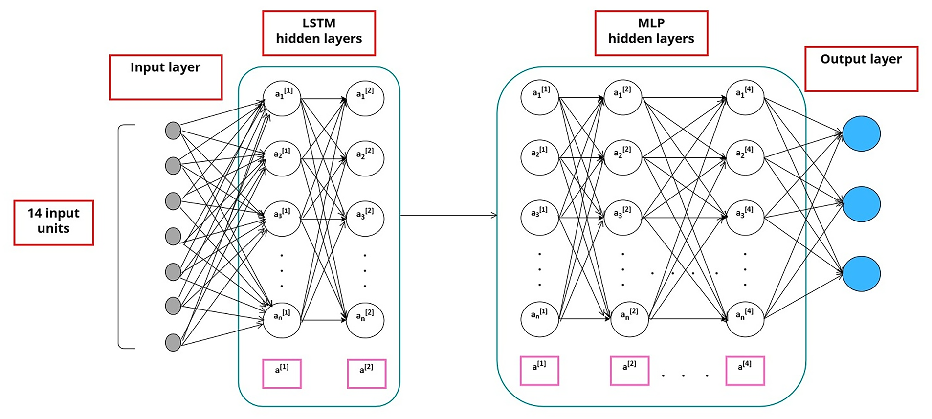
Figure 5: Schematic diagram of HS-LSTM-MLP.
2.6.2 Choice of HS-LSTM-MLP Structural Parameters
The proposed hybrid model integrated two stacked LSTM layers, each containing 128 hidden units, followed by a Multilayer Perceptron (MLP) block composed of four fully connected layers with 384, 256, 128, and 128 neurons, respectively. Each MLP layer was followed by a ReLU activation function to introduce non-linearity. The network began with an input layer consisting of fourteen nodes, corresponding to the raw sagittal-plane marker trajectories of the hip, knee, and ankle, thigh and shank segment velocities, and thigh and shank unit-vector rates. It concluded with a single-node output layer representing the predicted knee joint angle. To enhance the model’s generalization capability, a dropout layer with a dropout rate of 0.3 was incorporated. The output layer employed a regression layer to produce the final continuous joint angle prediction. The Hybrid Stacked LSTM-MLP (HS-LSTM-MLP) model was trained using the state-of-the-art Adam optimization algorithm over 100 epochs. The learning rate was initialized at 0.005, with a drop factor of 0.3. A mini-batch size of 1024 was used during training. The designed HS-LSTM-MLP architecture is presented in Fig. 6.
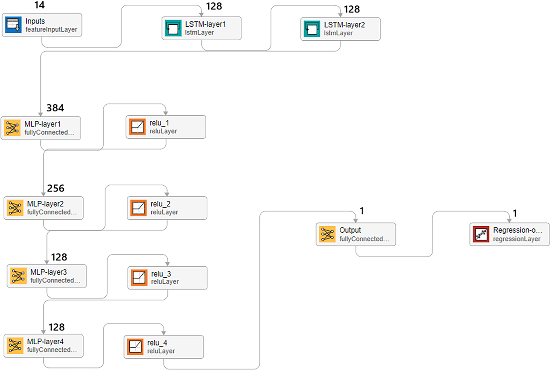
Figure 6: HS-LSTM-MLP architecture.
For all the models’ evaluation, the dataset was divided using a participant-wise strategy, where 90% (18) of participants were used for training, and the remaining 10% (2) were reserved for testing. After splitting, standardizing (z-score) input features using global mean and standard deviation ensured feature comparability across surfaces, legs, and subjects [30,53]. The split was performed before sequence generation to ensure that no overlapping windows or temporally adjacent frames from the same participant appeared in both training and testing sets. This approach was adopted to avoid information leakage caused by temporal autocorrelation between neighbouring gait frames.
To assess inter-subject generalization, leave-one-subject-out (LOSO) cross-validation was performed deploying HS-LSTM-MLP model. For each iteration, one participant was selected as the test subject, while the remaining participants were used for training. This procedure was repeated until every participant served once as the unseen test subject. Z-score normalization was performed within each fold using only the training participants, and the same normalization parameters were applied to the test participant.
It is demonstrated that knee joint angle estimation based on marker-derived features is well suited for prosthesis control and can ameliorate knee joint angle estimation accuracy with the proposed method. Marker data from 19 different anatomical locations were collected and used to compute knee joint kinematics. Features derived from hip, knee, and ankle markers are used as inputs to the machine learning models, while the corresponding calculated knee joint angles served as output variables. The reported performance metrics are obtained using a participant-wise data partition in which data from 18 participants (90%) are used for training, and the remaining two participants (10%) are reserved exclusively for testing. The split is performed before sequence generation; therefore, no temporally adjacent frames or overlapping windows from the same participant are shared between the training and testing sets. This evaluation protocol prevents information leakage arising from temporal autocorrelation and ensures that all reported test results correspond to previously unseen participants. Marker-based knee joint angle estimation is assessed by comparing four different types of deep neural networks: HS-LSTM-MLP, BiLSTM, LSTM, and MLP. Fig. 7 represents the comparison of actual vs. predicted knee joint angles through four neural networks, over five surfaces: level ground, ramp ascent, ramp descent, stair ascent, and stair descent. HS-LSTM-MLP model results are found most accurate and reliable for knee joint angle estimation when compared to other models. By comparing the angle prediction results, it is analyzed whether the application of the marker data alone could enhance knee joint angle prediction.
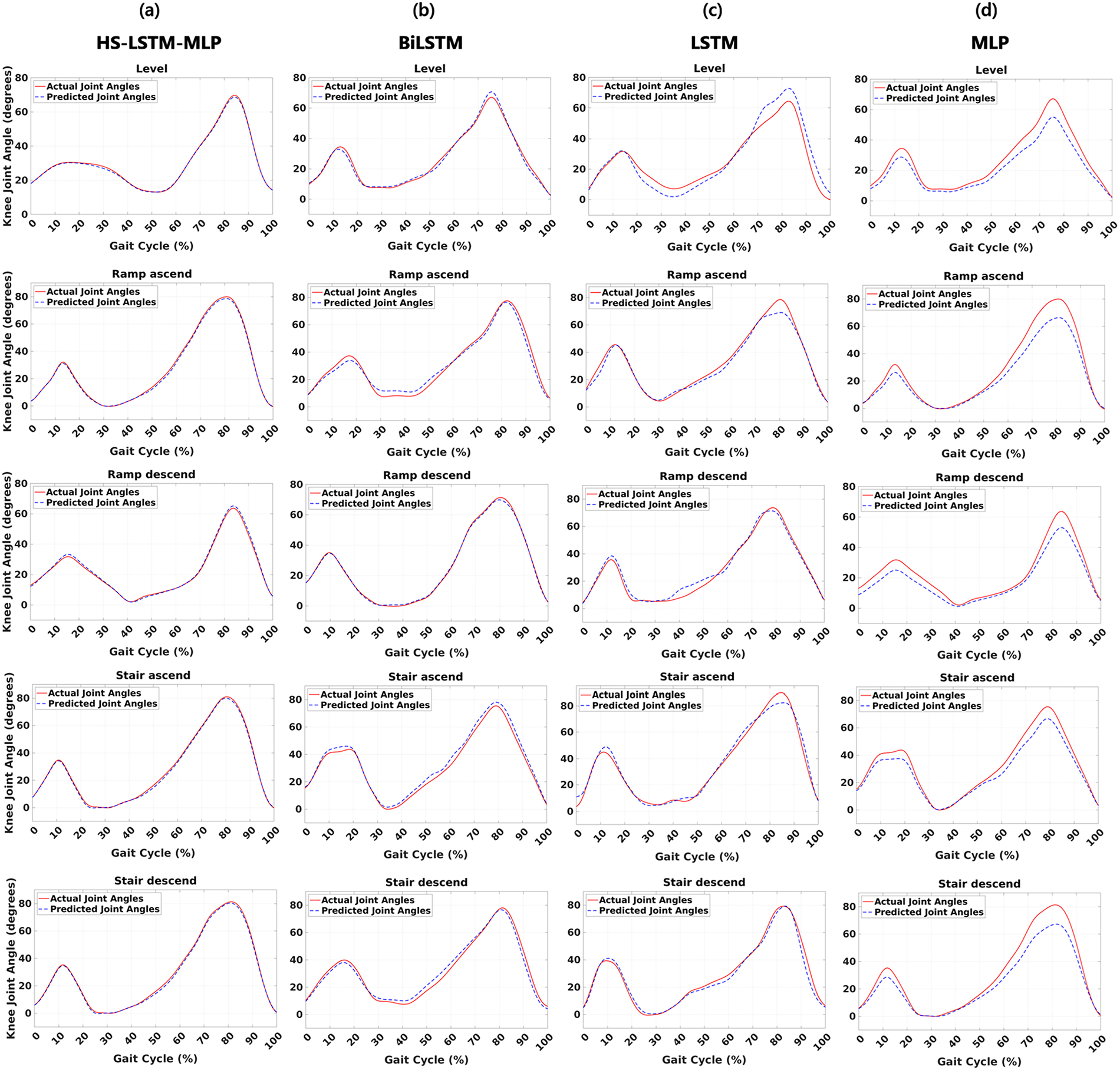
Figure 7: Actual vs. predicted knee joint angle curve over five different surfaces, with (a) HS-LSTM-MLP, (b) BiLSTM, (c) LSTM, and (d) MLP.
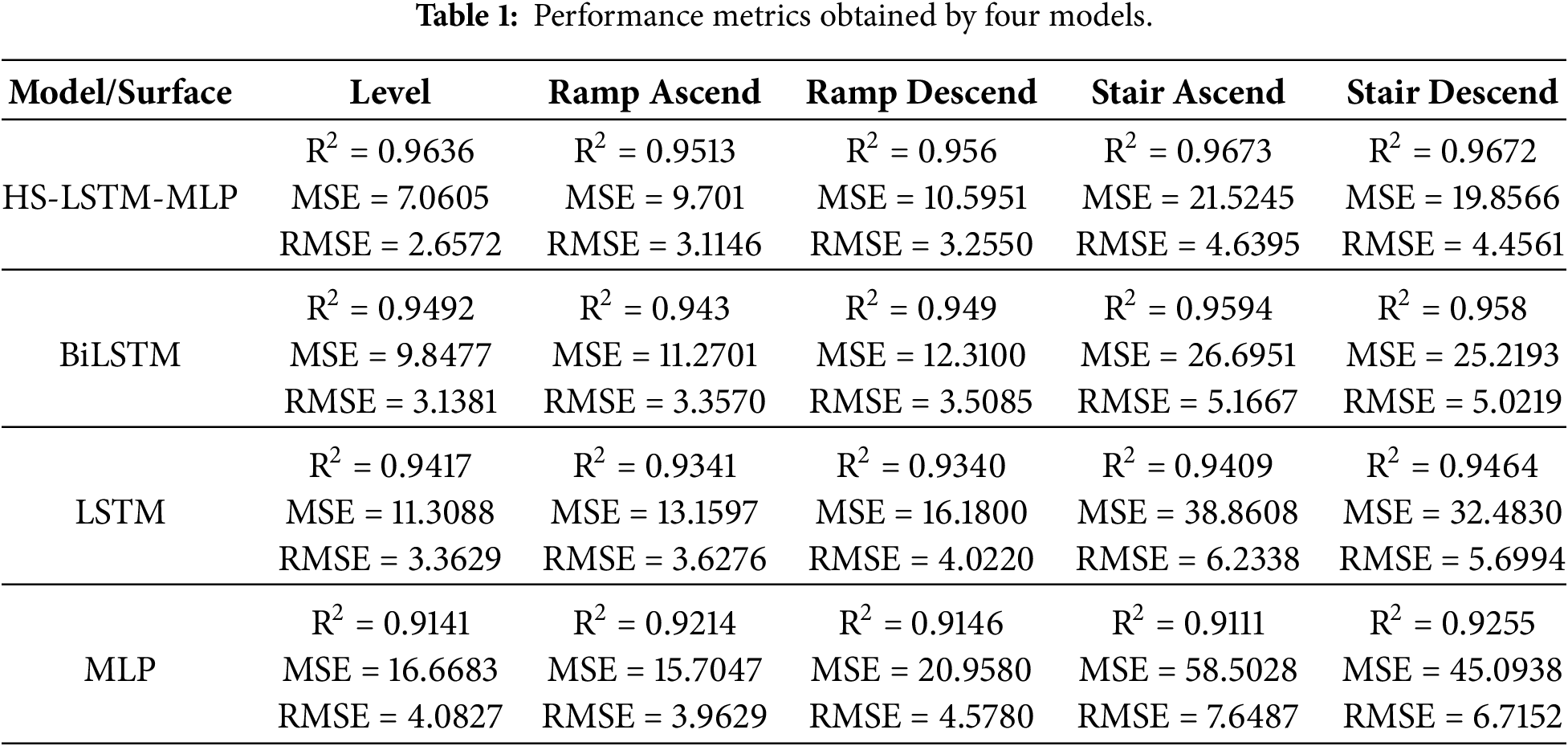
Regression performance is primarily quantified using the root mean square error (RMSE) and coefficient of determination (R2), which are commonly adopted metrics for continuous prediction tasks [54]. Prediction accuracy is generally considered poor when RMSE exceeds 9° or when the coefficient of determination R2 falls below 0.60 [2,11]. In addition to RMSE and R2, the performance of HS-LSTM-MLP, BiLSTM, LSTM and MLP networks in the prediction task is comprehensively appraised by employing additional metrics and mean squared error (MSE). Performance metrics are evaluated individually for five surfaces, since different gait dynamics are associated with different surfaces. The HS-LSTM-MLP network significantly outperforms BiLSTM, LSTM, and MLP networks in predicting the required knee kinematics for a walking time of 120 s. When using the HS-LSTM-MLP network, the largest errors occurred during stair ascent, with MSE of 21.5245 and RMSE of 4.6395°. The performance of the HS-LSTM-MLP network, as assessed by the R2, MSE, and RMSE, is found to have sufficient efficiency, as compared with BiLSTM, LSTM, and MLP, as presented in Table 1.
The preprocessing of the signals and all analyses are done in MATLAB R2024b [55]. The computer, which contains Intel(R) Core (TM) i7-1255U CPU@1.70 GHz processors, is used to train the networks.
To further evaluate subject independence, leave-one-subject-out (LOSO) cross-validation was performed using the HS-LSTM-MLP model. In each fold, one participant is held out for testing while the remaining participants are used for training. This process is repeated until every participant serves once as the unseen test participant. The mean LOSO evaluation results are presented in Table 2. These results demonstrate that the proposed model maintains strong predictive performance when evaluated on participants that are entirely unseen during training, thereby supporting its inter-subject generalization capability.
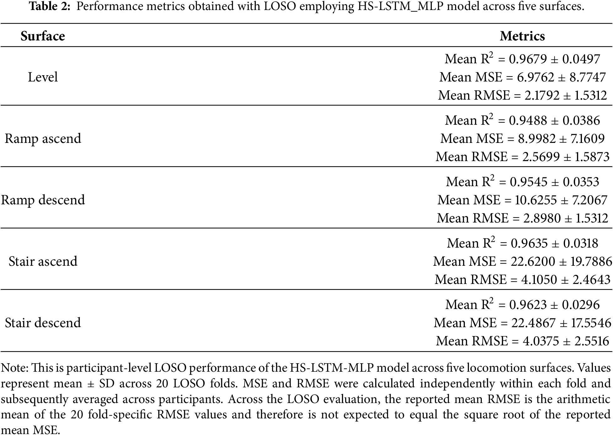
The LOSO evaluation produced performance that is consistent with the participant-wise 90%/10% split, with comparable R2 and RMSE values. The close agreement between the two validation strategies indicates that the proposed HS-LSTM-MLP model maintains stable predictive accuracy when applied to participants that are entirely unseen during training. These findings demonstrate the proficiency of the proposed model and provide strong evidence of its inter-subject generalization capability.
Normally, knee joint angles are represented as a function of the gait cycle. Knee joint angles predicted by four models are illustrated in Fig. 8, where all four estimation models’ curves are plotted together along with the actual knee joint angle curve. It clearly reflects the validity of the proposed model HS-LSTM-MLP, as its curve (black dotted line) follows most closely the actual knee joint angle curve (red solid curve), and the MLP (purple dotted curve) curve lags most behind.
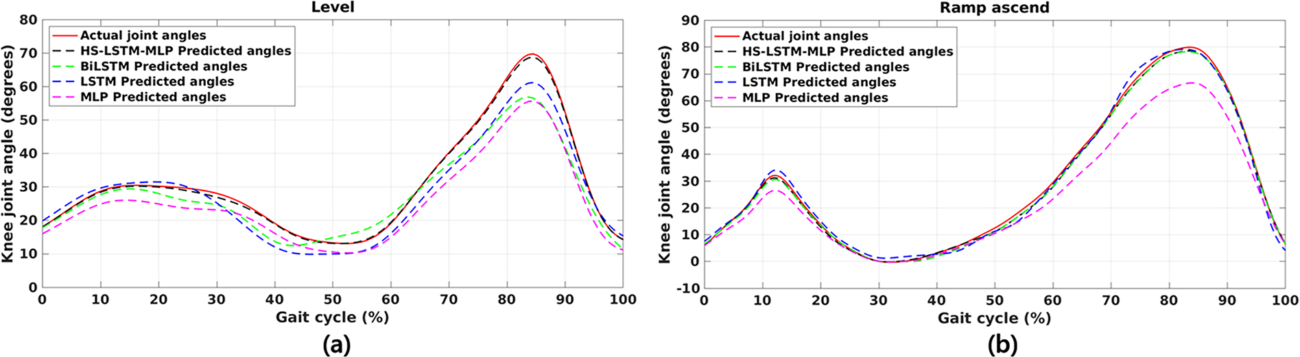
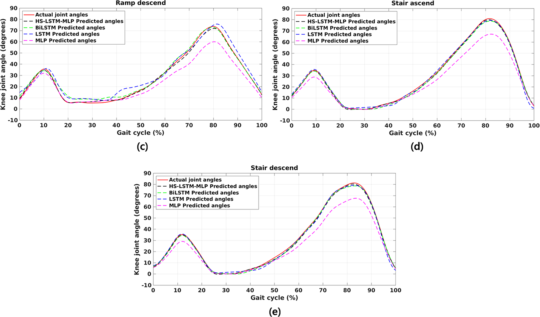
Figure 8: Comparison of four prediction models across: (a) level ground, (b) ramp ascend, (c) ramp descend, (d) stair ascend, and (e) stair descend.
Standard deviation in R2 and RMSE is computed across each surface, for 20 participants, and error bars in Figs. 9 and 10 display standard deviations for the respective R2 and RMSE. It is evident from the figures that there is less variation in HS-LSTM-MLP results, as compared with BiLSTM, LSTM, and MLP models.
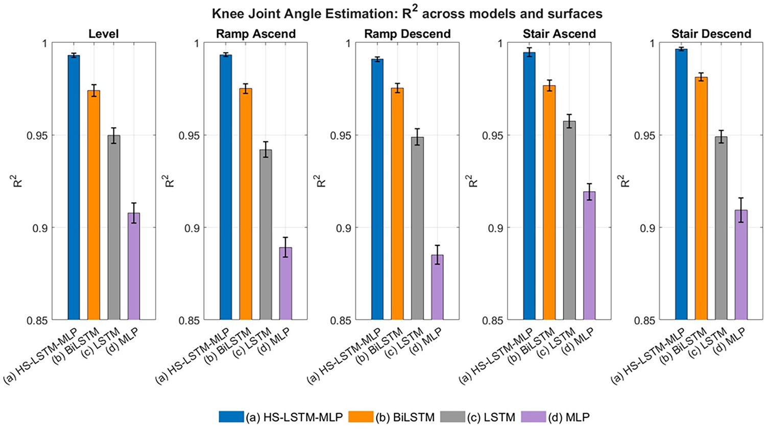
Figure 9: Standard deviation in R2 across 20 participants for (a) HS-LSTM-MLP, (b) BiLSTM, (c) LSTM and (d) MLP models over five walking surfaces.
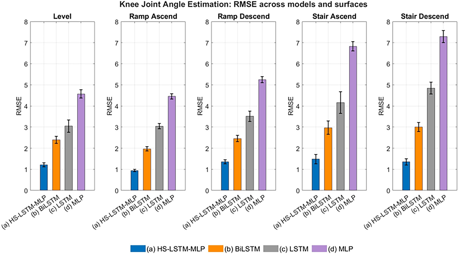
Figure 10: Standard deviation in RMSE across 20 participants for (a) HS-LSTM-MLP, (b) BiLSTM, (c) LSTM and (d) MLP models over five walking surfaces.
To determine whether the observed performance differences among HS-LSTM-MLP, BiLSTM, LSTM, and MLP are statistically significant, a Friedman test is performed separately for each locomotion surface using the participant-level R2 and RMSE values (n = 20). When the Friedman test indicates a significant overall difference, post-hoc pairwise Wilcoxon signed-rank tests with Holm-Bonferroni correction are conducted to compare the proposed HS-LSTM-MLP model against the baseline models. The statistical analysis results are summarized in Table 3.
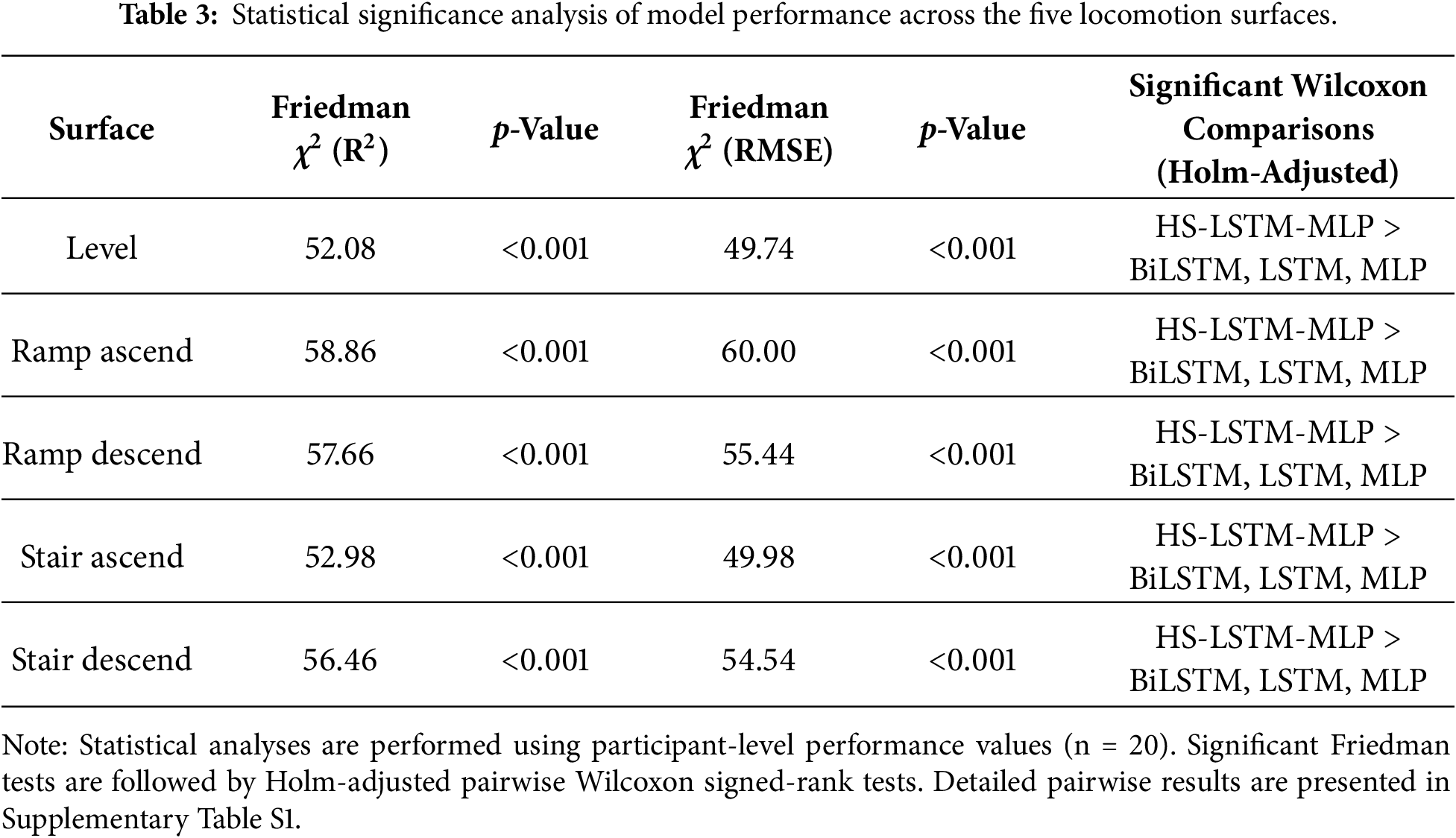
As summarized in Table 3, the Friedman test reveals statistically significant differences among the four models for both R2 and RMSE across all five locomotion surfaces (all p < 0.001). The statistical analysis is performed using participant-level performance values. Significant omnibus results are followed by pairwise Wilcoxon signed-rank tests with Holm–Bonferroni correction, which confirms that the proposed HS-LSTM-MLP model significantly outperformed the BiLSTM, LSTM, and MLP models across all locomotion surfaces for both evaluation metrics. These findings provide statistical evidence supporting the superior performance of the proposed model. Detailed Holm-adjusted p-values and matched-pairs rank-biserial effect sizes for all pairwise comparisons are provided in Supplementary Table S1.
This research examines knee joint kinematics across five locomotion surfaces commonly encountered in daily activities, with the aim of improving prosthetic control for transfemoral amputees. Considering multiple surfaces simultaneously remains relatively uncommon in knee-angle prediction studies, particularly with the level of accuracy achieved here. Previous studies typically report RMSE values ranging from 2° to 9° and R2 values between 0.7 and 0.95 for knee-angle estimation during various activities such as walking at different speeds, surface transitions, sit-to-stand motion, running, or jumping [11,34,40,41].
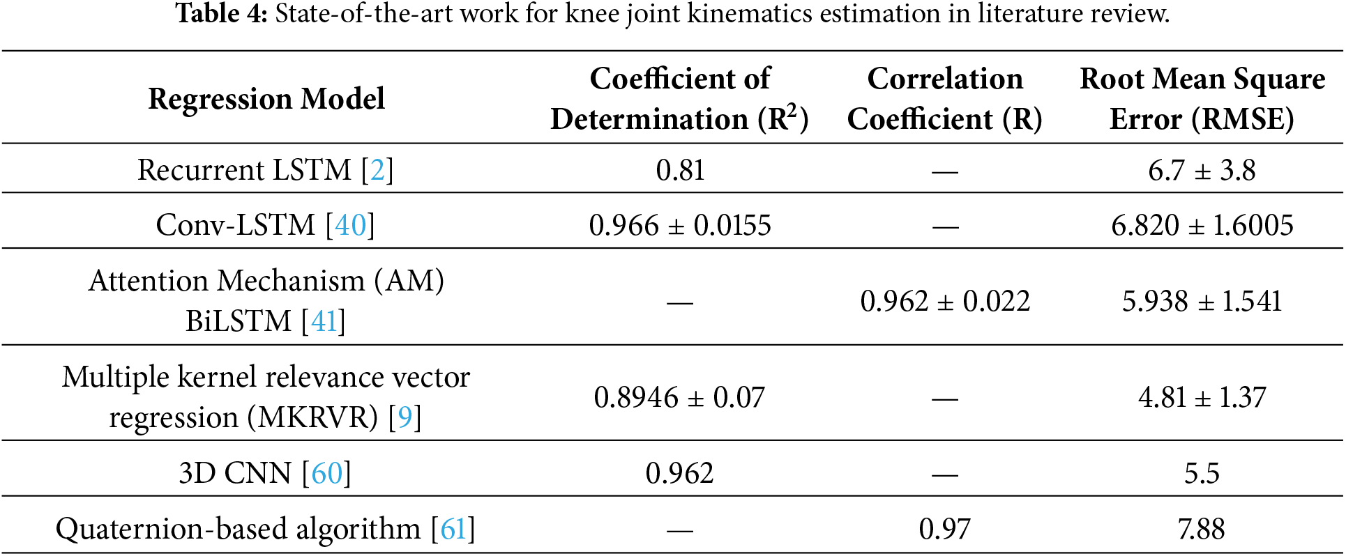
Previous studies have commonly evaluated knee joint angle estimation models using the performance metrics of RMSE and R2 (or R), with many reported RMSE values exceeding 3° [56–59]. Table 4 summarizes the performance of representative machine learning regression models for knee joint angle prediction reported in the literature. For instance, one study predicted knee joint kinematics using motion capture and IMU data with a recurrent LSTM model, achieving an RMSE of 6.7 ± 3.8° and an R2 of 0.81 [2]. Similarly, Lu et al. [40] investigated the prediction of lower-limb joint kinematics during multiple functional activities, including walking, running, stair ascent, stair descent, sit-to-stand, stand-to-sit, and jumping. Their Conv-LSTM model achieved the highest accuracy for knee joint prediction during the sit-to-stand task, with an R2 of 0.966 ± 0.0155. Likely, Zangene et al. [41] investigated knee joint kinematics during walking at different speeds and reported the highest prediction accuracy at a walking speed of 2 m/s, achieving a correlation coefficient of R = 0.962 ± 0.022. Additionally, another study proposed a novel Multi-Kernel Relevance Vector Regression (MKRVR) model for offline knee joint angle prediction, reporting an R2 of 0.8946 ± 0.07 and an RMSE of 4.81 ± 1.37° [9]. Wei et al. [60] further employed a three-dimensional convolutional neural network (3D-CNN) for knee joint kinematics estimation, achieving an R2 of 0.962 with an RMSE of 5.5°. In another approach, an orientation-estimation algorithm based on quaternion calculations was developed to estimate the orientation of wearable sensor units, which was subsequently transformed into body-segment orientations for gait analysis and validated against a camera-based motion capture system. This method achieved a correlation coefficient of 0.97 with an RMSE of 7.88° [61].
The proposed HS-LSTM-MLP network produces the most precise estimates of knee joint kinematics across all surfaces, outperforming all BiLSTM, LSTM and MLP networks. The highest R2 values obtained with HS-LSTM-MLP (R2 in the range 0.9513–0.9673) indicate an almost perfect agreement between predicted and reference knee joint angles, demonstrating the model’s capability to capture the nonlinear relationship between marker-derived features and joint motion. In comparison, MLP shows far less performance, with R2 in the range 0.9111–0.9255 and the highest MSE (15.7047–58.5028) and RMSE (3.9629–7.6487) as compared to all four models. LSTM model, although showing comparatively better performance (R2 in the range 0.9340–0.9464), still exhibited larger deviations, reflected by higher MSE (11.3088–38.8608) and RMSE (3.3629°–6.2338°). The BiLSTM model shows better performance than LSTM and MLP networks. Comparison of performance metrics of four models across five surfaces is presented in Fig. 11.
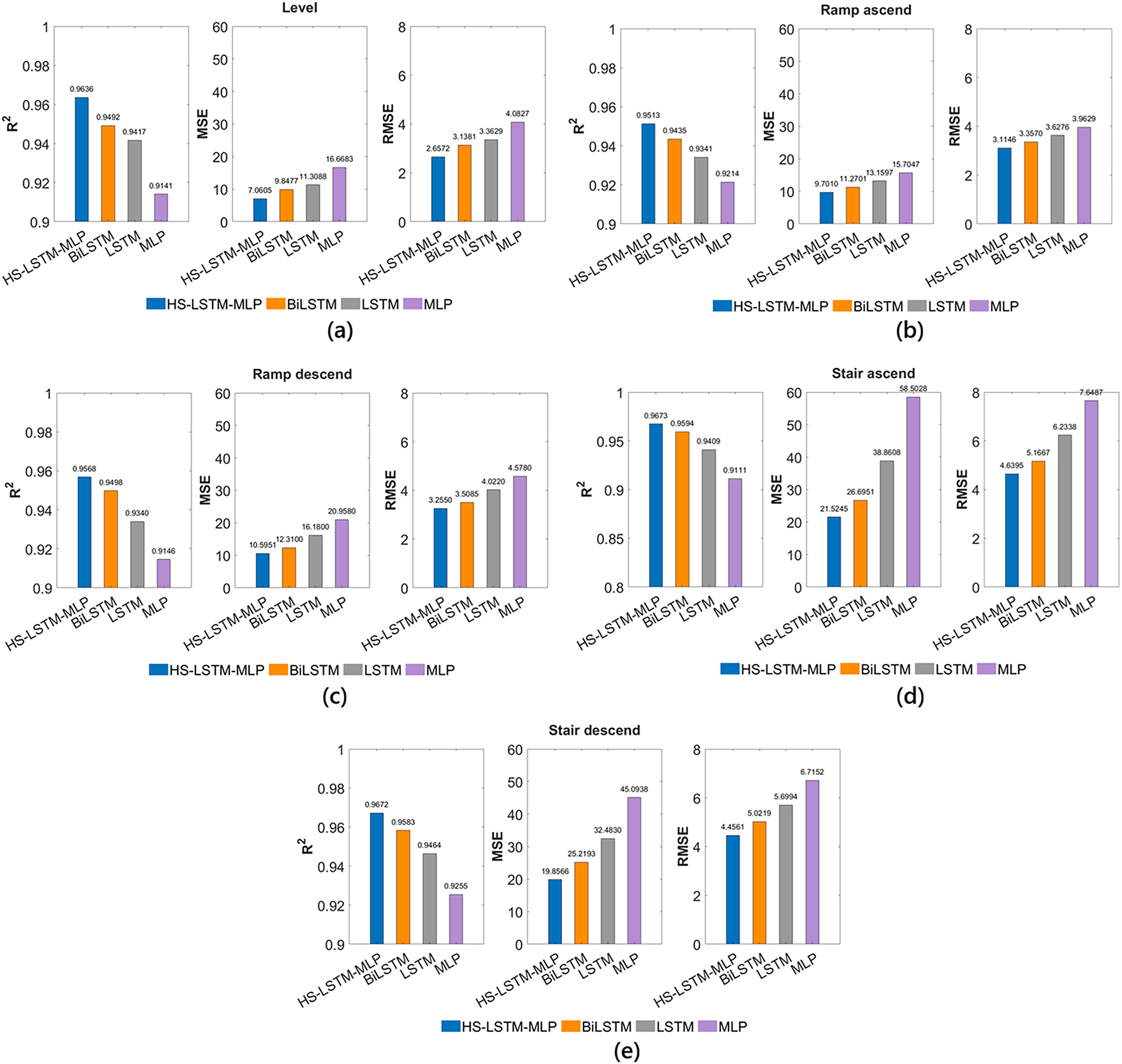
Figure 11: Performance metrics comparison of four models over five surfaces: (a) level ground, (b) ramp ascend, (c) ramp descend, (d) stair ascend, and (e) stair descend.
The consistent ranking of model performance, followed by BiLSTM, LSTM, and MLP across all locomotion surfaces, indicates the superior predictive capability of the proposed hybrid architecture. Although isolated variations were observed in MSE and RMSE on certain surfaces, the overall statistical analysis demonstrated that HS-LSTM-MLP achieved significantly better performance than the comparison models. The stacked LSTM layers provide sufficient temporal awareness without the instability associated with deep recurrent loops, while the multilayer perceptron component enables efficient nonlinear regression and dense feature abstraction. This balance likely contributes to the superior representational capability and generalisation observed across different surfaces.
BiLSTM provides enhanced sequence representation by incorporating past and future temporal contexts; its non-causal nature may limit direct implementation in real-time prosthetic controllers where future gait information is unavailable. Therefore, BiLSTM is considered a performance comparison model rather than a real-time control solution. Future work will include detailed computational benchmarking, including inference latency, model complexity, memory usage, and embedded hardware validation to evaluate practical deployment feasibility. A standard LSTM network shows lower performance, possibly due to its unidirectional structure, which restricts access to future temporal context. In addition, recurrent networks can still suffer from gradient degradation during training, potentially affecting long-term learning stability. The MLP model demonstrates effective nonlinear mapping capability; however, its feedforward structure processes input features independently and lacks an inherent mechanism to capture temporal dependencies within sequential gait data. Consequently, MLP performance may be limited for dynamic knee kinematics estimation, where current joint motion is influenced by previous movement patterns.
From a biomechanical perspective, the results suggest that knee motion across walking surfaces is highly nonlinear but only moderately dependent on long-range temporal context. Consequently, architectures emphasising nonlinear feature learning combined with moderate temporal modelling, such as HS-LSTM-MLP, appear well suited to this problem. The very low RMSE (<4.6395°) achieved by HS-LSTM-MLP across all surfaces indicates strong potential for prosthetic applications, where angular precision within a few degrees is considered clinically acceptable. The close alignment between predicted and actual trajectories also indicates minimal phase delay, an important requirement for reliable prosthetic control.
Error trends further demonstrate that HS-LSTM-MLP not only reduced mean prediction error but also minimised inter-participant variability. Consistently low MSE values (<21.5245) compared with BiLSTM (<26.6951), LSTM (<38.8608) and MLP (<58.5028) suggest improved response to unseen gait conditions. The narrow distribution of R2 values across surfaces supports the conclusion that HS-LSTM-MLP captures intrinsic biomechanical motion patterns rather than surface-specific noise. In contrast, MLP exhibits the highest prediction errors and variability because its feedforward architecture lacks an inherent mechanism for modelling temporal dependencies, limiting its ability to capture the sequential characteristics of gait motion. The larger variability observed for LSTM indicates greater sensitivity to sequence-length variations and input disturbances. BiLSTM partially mitigates this limitation through bidirectional context modelling, explaining its intermediate performance.
These findings reinforce the importance of selecting an appropriate architecture for gait-kinematics prediction. Although recurrent models are widely used for time-series analysis, their advantages may diminish when temporal continuity is less dominant than spatial structure and statistical relationships in the input data. Hybrid feedforward-dominant architectures with hierarchical feature learning may therefore offer a more efficient solution for biomechanical regression tasks, particularly when signals are carefully filtered, normalised, and temporally aligned.
The predictive accuracy achieved by HS-LSTM-MLP is comparable to that reported in much of the recent literature on knee angle estimation, [2,9,40,41,60] where standalone LSTM-based methods typically report RMSE values between 2° and 9° and R2 values of 0.81–0.96 depending on sensor modality and task complexity [2,40,41]. The improved performance observed here likely stems from the combination of structured spatial-temporal features, low-pass filtering of marker trajectories to suppress high-frequency noise, and carefully optimised network depth and neuron distribution.
While many previous studies rely on sEMG or IMU sensors for intent recognition and joint prediction, the present study demonstrates that accurate knee-angle estimation can be achieved from reflective marker trajectories under controlled laboratory conditions. This marker-based proof-of-concept provides a reliable framework for investigating biomechanical relationships and developing predictive models using high-fidelity kinematic measurements. Accordingly, the proposed approach is well suited for clinical gait analysis and rehabilitation research, where optical motion-capture systems remain the reference standard. However, reflective marker systems are not intended for real-world prosthetic control, and future work will investigate transferring the proposed modelling framework to wearable sensing modalities, such as IMUs or sEMG, for practical deployment.
Although the present study was conducted using motion capture data from healthy participants under controlled laboratory conditions, the findings provide a proof-of-concept for accurate marker-based knee joint kinematics estimation that may inform the future development of adaptive transfemoral prosthetic control systems. Accurate prediction of knee joint kinematics is an important prerequisite for achieving stable locomotion across varied walking surfaces, particularly ramps and stairs, which remain challenging environments for transfemoral prosthesis users. The proposed HS-LSTM-MLP model demonstrated strong predictive capability, reliable performance, and responsiveness to noise in healthy gait, suggesting its potential as a biomechanical prediction framework for future prosthetic applications. However, clinical validation in individuals with lower-limb amputation is required before its suitability for prosthetic control can be established. Future work will integrate this proposed marker-based knee joint kinematics estimation framework with an automatic sEMG-based surface recognition system to enable real-time adaptive locomotion analysis across multiple walking environments.
A notable limitation encountered during data collection was the occlusion of foot markers during stair ascent and descent. Because of the geometric configuration of the staircase, the reflective markers placed on the foot, particularly those located on the heel and toe, were frequently hidden behind the stair edges during the swing and stance phases. This occlusion resulted in intermittent marker loss, leading to incomplete or noisy trajectories within the captured motion data. Missing foot-marker information disrupted the continuity of the lower-limb kinematic chain and adversely affected the reconstruction of gait dynamics, particularly for joints whose motion depends on accurate foot placement and orientation. Although gap-filling procedures and interpolation strategies were applied to mitigate these effects, the loss of marker visibility remained an inherent challenge in optical motion-capture systems. Another limitation is that 3D/2D kinematics from external sources like reflective markers are unlikely for the control of a prosthesis in real-life. However, with ML models like the one proposed here, it may be possible to implement with other types of inputs like IMU or sEMG, at the time of implementation. Also, this study focused exclusively on sagittal-plane kinematics; therefore, the proposed algorithms do not account for movements in the frontal and transverse planes. While sagittal-plane motion is the primary contributor to forward propulsion during gait, movements in the other planes—particularly in the frontal (mediolateral) direction—play an important role in balance and stability. Consequently, the exclusion of frontal and transverse plane dynamics may limit the ability of the model to fully capture aspects of balance control, including those associated with fall risk.
A notable limitation of this study is that the motion capture data were collected exclusively from healthy participants with intact lower limbs under controlled laboratory conditions. Consequently, although the proposed HS-LSTM-MLP model demonstrated promising performance for knee joint kinematics estimation, its direct applicability to individuals with lower-limb amputation has not yet been established. The gait biomechanics and movement patterns of prosthesis users differ substantially from those of able-bodied individuals due to altered neuromuscular control, residual-limb characteristics, prosthetic components, and compensatory gait strategies. Therefore, the present findings should be interpreted as a proof-of-concept for marker-based knee joint kinematics estimation rather than a clinically validated prosthetic control solution.
This study focused exclusively on knee joint kinematics estimation with the novel hybrid model. Future research can extend the model to estimate multi-joint kinematics, including hip and ankle angles, enabling full lower-limb motion reconstruction, and even on upper limb. This would greatly enhance the applicability of the system in gait assessment, prosthesis control, and rehabilitation robotics. Additionally, this model is evaluated offline in MATLAB; future work should focus on real-time deployment of the HS-LSTM-MLP model on an embedded platform. Low-latency implementation would allow real-time knee-angle prediction for prosthesis control. Moreover, future studies will perform detailed component-level ablation experiments to systematically investigate the effects of network depth, feature selection, regularization strategies, and optimization parameters on model performance and computational efficiency.
Future studies will validate the proposed HS-LSTM-MLP framework using gait data collected from individuals with transfemoral amputation under clinically relevant conditions. The model will be adapted to account for amputee-specific gait characteristics and prosthetic biomechanics, thereby improving its clinical applicability. In addition, future work will investigate the integration of automatic surface recognition and multimodal sensing to enable adaptive, real-time prosthetic control across diverse locomotion environments. Moreover, future research may explore multimodal hybrid frameworks combining MLP-based feature extraction with lightweight temporal modules such as gated recurrent units (GRUs) or temporal convolutional networks (TCNs), which could preserve temporal interpretability while maintaining prediction accuracy.
This study demonstrates a practical approach to predicting knee joint angles relying solely on the kinematic signals collected from reflective markers within a motion capture system. This proposed HS-LSTM-MLP model was evaluated against BiLSTM, LSTM, and MLP neural networks. It consistently achieved superior performance across all evaluation metrics. The HS-LSTM-MLP model provided accurate and reliable knee joint kinematics tracking for five surfaces, including level ground, ramp ascent, ramp descent, stair ascent, and stair descent. The performance metrics employed here are R2, MSE, and RMSE to compare the performance of the proposed HS-LSTM-MLP network, where HS-LSTM-MLP surpasses the performance of all three BiLSTM, LSTM, and MLP networks. This architecture has proved to be accurate and efficient in the inter-subject knee joint kinematics prediction task. Overall, the proposed method offers a promising solution for transfemoral prosthetic knee joint control over various surfaces, while also providing potential applications in clinical gait analysis, rehabilitation, and diagnosis of knee joint disorders.
Acknowledgement: This project was supported by Swinburne University of Technology, Melbourne, Australia. And the data collection was supported by Biomechanics lab staff in Swinburne University of Technology, Melbourne, Australia namely Jesús Campo Uribe, Ashlee Hope, Matthew Rudden, and Rebecca Battersby.
Funding Statement: This research was funded by Swinburne University of Technology, Melbourne, Australia.
Author Contributions: The authors confirm contribution to the paper as follows: Conceptualization, Faiza Rasheed, Jinchuan Zheng and Kwong Ming Tse; methodology, Faiza Rasheed, Jinchuan Zheng, Luis Eduardo Cofré Lizama and Kwong Ming Tse; software, Faiza Rasheed, Jinchuan Zheng and Suzanne Martin; validation, Faiza Rasheed; formal analysis, Faiza Rasheed; investigation, Faiza Rasheed, Jinchuan Zheng and Kwong Ming Tse; resources, Luis Eduardo Cofré Lizama and Kwong Ming Tse; data curation, Faiza Rasheed, Luis Eduardo Cofré Lizama and Suzanne Martin; writing—original draft preparation, Faiza Rasheed; writing—review and editing, Jinchuan Zheng, Luis Eduardo Cofré Lizama and Kwong Ming Tse; visualization, Faiza Rasheed and Jinchuan Zheng; supervision, Jinchuan Zheng, Luis Eduardo Cofré Lizama and Kwong Ming Tse; project administration, Kwong Ming Tse; funding acquisition, Kwong Ming Tse. All authors reviewed and approved the final version of the manuscript.
Availability of Data and Materials: The data that supports the findings of this study are not publicly available due to ethical restrictions and confidentiality agreements. Access to the data is limited to the research team and cannot be shared in a public repository.
Ethics Approval: This research involving humans was approved by Swinburne University of Technology Human Research Ethics Committee (SUHREC), Australia (Reference no: 20246933-17851 and date of approval: March 6th, 2024). The research was conducted in accordance with the institutional requirements. The participants provided their written informed consent to participate in this research. Written informed consent was obtained from the individuals for the publication of any images or data included in this article.
Conflicts of Interest: The authors declare no conflicts of interest.
Supplementary Materials: The supplementary material is available online at https://www.techscience.com/doi/10.32604/cmes.2026.086130/s1.
Abbreviations:
The following abbreviations are used in this manuscript
| LSTM | Long Short-Term Memory |
| BiLSTM | Bidirectional Long Short-Term Memory |
| MLP | Multilayer Perceptron |
| HS-LSTM-MLP | Hybrid Stacked Long Short-Term Memory-Multilayer Perceptron |
| IMU | Inertial Measurement Unit |
| sEMG | Surface Electromyography |
| R2 | Coefficient of Determination |
| RMSE | Root Mean Square Error |
References
1. Windrich M, Grimmer M, Christ O, Rinderknecht S, Beckerle P. Active lower limb prosthetics: a systematic review of design issues and solutions. BioMedical Eng OnLine. 2016;15(3):140. doi:10.1186/s12938-016-0284-9. [Google Scholar] [CrossRef]
2. Bian Q, Castellani M, Shepherd D, Duan J, Ding Z. Gait intention prediction using a lower-limb musculoskeletal model and long short-term memory neural networks. IEEE Trans Neural Syst Rehabil Eng. 2024;32:822–30. doi:10.1109/TNSRE.2024.3365201. [Google Scholar] [CrossRef]
3. Wang F, Liang W, Afzal HMR, Fan A, Li W, Dai X, et al. Estimation of lower limb joint angles and joint moments during different locomotive activities using the inertial measurement units and a hybrid deep learning model. Sensors. 2023;23(22):9039. doi:10.3390/s23229039. [Google Scholar] [CrossRef]
4. Zhang L, Liu G, Han B, Wang Z, Yan Y, Ma J, et al. Knee joint biomechanics in physiological conditions and how pathologies can affect it: a systematic review. Appl Bionics Biomech. 2020;2020(1):7451683. doi:10.1155/2020/7451683. [Google Scholar] [CrossRef]
5. Liang W, Qian Z, Chen W, Song H, Cao Y, Wei G, et al. Mechanisms and component design of prosthetic knees: a review from a biomechanical function perspective. Front Bioeng Biotechnol. 2022;10:950110. doi:10.3389/fbioe.2022.950110. [Google Scholar] [CrossRef]
6. Rasheed F, Martin S, Tse KM. Design, kinematics and gait analysis, of prosthetic knee joints: a systematic review. Bioengineering. 2023;10(7):773. doi:10.3390/bioengineering10070773. [Google Scholar] [CrossRef]
7. Weber JG, Ortigas-Vásquez A, Sauer A, Dupraz I, Utz M, Maas A, et al. Comparison of IMU-based knee kinematics with and without harness fixation against an optical marker-based system. Bioengineering. 2024;11(10):976. doi:10.3390/bioengineering11100976. [Google Scholar] [PubMed] [CrossRef]
8. Cheng S, Bolívar-Nieto E, Welker CG, Gregg RD. Modeling the transitional kinematics between variable-incline walking and stair climbing. IEEE Trans Med Robot Bionics. 2022;4(3):840–51. doi:10.1109/tmrb.2022.3185405. [Google Scholar] [CrossRef]
9. Li HB, Guan XR, Li Z, Zou KF, He L. Estimation of knee joint angle from surface EMG using multiple kernels relevance vector regression. Sensors. 2023;23(10):4934. doi:10.3390/s23104934. [Google Scholar] [CrossRef]
10. Fernández-González C, De la Calle B, Gómez C, Saoudi H, Iordanov D, Cenni F, et al. Estimating gait kinematics from muscle activity using deep learning in typically developing children. BioRxiv:703957. 2026. doi:10.64898/2026.02.05.703957. [Google Scholar] [CrossRef]
11. Ma X, Liu Y, Song Q, Wang C. Continuous estimation of knee joint angle based on surface electromyography using a long short-term memory neural network and time-advanced feature. Sensors. 2020;20(17):4966. doi:10.3390/s20174966. [Google Scholar] [CrossRef]
12. Cavanagh PR, Komi PV. Electromechanical delay in human skeletal muscle under concentric and eccentric contractions. Eur J Appl Physiol Occup Physiol. 1979;42(3):159–63. doi:10.1007/BF00431022. [Google Scholar] [CrossRef]
13. Roland T, Wimberger K, Amsuess S, Russold MF, Baumgartner W. An insulated flexible sensor for stable electromyography detection: applicationto prosthesis control. Sensors. 2019;19(4):961. doi:10.3390/s19040961. [Google Scholar] [CrossRef]
14. Krieger KJ, Lijnse TM, Lowery MM, O’Cearbhaill ED. Microneedle electrodes for electromyography. Biosens Bioelectron. 2025;290:117945. doi:10.1016/j.bios.2025.117945. [Google Scholar] [CrossRef]
15. Li N, Zhou R, Krishna B, Pradhan A, Lee H, He J, et al. Non-invasive techniques for muscle fatigue monitoring: a comprehensive survey. ACM Comput Surv. 2024;56(9):1–40. doi:10.1145/3648679. [Google Scholar] [CrossRef]
16. Tan JS, Tippaya S, Binnie T, Davey P, Napier K, Caneiro JP, et al. Predicting knee joint kinematics from wearable sensor data in people with knee osteoarthritis and clinical considerations for future machine learning models. Sensors. 2022;22(2):446. doi:10.3390/s22020446. [Google Scholar] [CrossRef]
17. Al-Rashdan A, Amari H, Al-Smadi Y. Long short-term memory network for contralateral knee angle estimation during level-ground walking: a feasibility study on able-bodied subjects. Micromachines. 2026;17(2):157. doi:10.3390/mi17020157. [Google Scholar] [CrossRef]
18. Ackland DC, Fang Z, Senanayake D. A machine learning approach to real-time calculation of joint angles during walking and running using self-placed inertial measurement units. Gait Posture. 2025;118:85–91. doi:10.1016/j.gaitpost.2025.01.028. [Google Scholar] [CrossRef]
19. Cornish BM, Diamond LE, Saxby DJ, Lloyd DG, Shi B, Lyon J, et al. Sagittal plane knee kinematics can be measured during activities of daily living following total knee arthroplasty with two IMU. PLoS One. 2024;19(2):e0297899. doi:10.1371/journal.pone.0297899. [Google Scholar] [CrossRef]
20. Wang S, Cai Y, Hase K, Uchida K, Kondo D, Saitou T, et al. Estimation of knee joint angle during gait cycle using inertial measurement unit sensors: a method of sensor-to-clinical bone calibration on the lower limb skeletal model. J Biomech Sci Eng. 2022;17(1):21–00196. doi:10.1299/jbse.21-00196. [Google Scholar] [CrossRef]
21. Molina-Rueda F, Fernández-González P, Cuesta-Gómez A, Koutsou A, Carratalá-Tejada M, Miangolarra-Page JC. Test-retest reliability of a conventional gait model for registering joint angles during initial contact and toe-off in healthy subjects. Int J Environ Res Public Health. 2021;18(3):1343. doi:10.3390/ijerph18031343. [Google Scholar] [CrossRef]
22. Harsted S, Holsgaard-Larsen A, Hestbæk L, Andreasen DL, Lauridsen HH. Test-retest reliability and agreement of lower-extremity kinematics captured in squatting and jumping preschool children using markerless motion capture technology. Front Digit Health. 2022;4:1027647. doi:10.3389/fdgth.2022.1027647. [Google Scholar] [CrossRef]
23. Wang S, Pitts J, Purohit R, Shah H. The influence of motion data low-pass filtering methods in machine-learning models. Appl Sci. 2025;15(4):2177. doi:10.3390/app15042177. [Google Scholar] [CrossRef]
24. Viswakumar A, Rajagopalan V, Ray T, Gottipati P, Parimi C. Development of a robust, simple, and affordable human gait analysis system using bottom-up pose estimation with a smartphone camera. Front Physiol. 2022;12:784865. doi:10.3389/fphys.2021.784865. [Google Scholar] [CrossRef]
25. Lavikainen J, Stenroth L, Vartiainen P, Alkjær T, Karjalainen PA, Henriksen M, et al. Predicting knee joint contact force peaks during gait using a video camera or wearable sensors. Ann Biomed Eng. 2024;52(12):3280–94. doi:10.1007/s10439-024-03594-x. [Google Scholar] [CrossRef]
26. Baček T, Sun M, Liu H, Chen Z, Manzie C, Burdet E, et al. A biomechanics and energetics dataset of neurotypical adults walking with and without kinematic constraints. Sci Data. 2024;11(1):646. doi:10.1038/s41597-024-03444-4. [Google Scholar] [CrossRef]
27. Kadaba MP, Ramakrishnan HK, Wootten ME. Measurement of lower extremity kinematics during level walking. J Orthop Res. 1990;8(3):383–92. doi:10.1002/jor.1100080310. [Google Scholar] [CrossRef]
28. Winter DA. Three-dimensional kinematics and kinetics. In: Biomechanics and motor control of human movement. Hoboken, NJ, USA: John Wiley & Sons, Inc.; 2009. p. 176–99. [Google Scholar]
29. Chen J, Mu X, Du F. Biomechanics analysis of human lower limb during walking for exoskeleton design. J Vibroeng. 2017;19(7):5527–39. doi:10.21595/jve.2017.18459. [Google Scholar] [CrossRef]
30. Roetenberg D, Luinge H, Slycke P. Xsens MVN: full 6DOF human motion tracking using miniature inertial sensors. Xsens Motion Technol BV Tech Rep. 2009: 1–7. [Google Scholar]
31. Kenas F, Saadia N, Ababou A, Ababou N, Zabat M, BenSiSaid K. Neural network-based estimation of lower limb joint kinematics: a minimally intrusive approach for gait analysis. Med Novel Technol Devices. 2024;23(11):100318. doi:10.1016/j.medntd.2024.100318. [Google Scholar] [CrossRef]
32. Fang Z, Woodford S, Senanayake D, Ackland D. Conversion of upper-limb inertial measurement unit data to joint angles: a systematic review. Sensors. 2023;23(14):6535. doi:10.3390/s23146535. [Google Scholar] [CrossRef]
33. Luinge HJ, Veltink PH. Measuring orientation of human body segments using miniature gyroscopes and accelerometers. Med Biol Eng Comput. 2005;43(2):273–82. doi:10.1007/BF02345966. [Google Scholar] [CrossRef]
34. Moghadam SM, Yeung T, Choisne J. A comparison of machine learning models’ accuracy in predicting lower-limb joints’ kinematics, kinetics, and muscle forces from wearable sensors. Sci Rep. 2023;13(1):5046. doi:10.1038/s41598-023-31906-z. [Google Scholar] [CrossRef]
35. Rácz K, Kiss RM. Marker displacement data filtering in gait analysis: a technical note. Biomed Signal Process Control. 2021;70:102974. doi:10.1016/j.bspc.2021.102974. [Google Scholar] [CrossRef]
36. Kim D, Kim DH, Kwak KC. Classification of K-pop dance movements based on skeleton information obtained by a kinect sensor. Sensors. 2017;17(6):1261. doi:10.3390/s17061261. [Google Scholar] [CrossRef]
37. Wu G, Siegler S, Allard P, Kirtley C, Leardini A, Rosenbaum D, et al. ISB recommendation on definitions of joint coordinate system of various joints for the reporting of human joint motion: part I: ankle, hip, and spine. International society of biomechanics. J Biomech. 2002;35(4):543–8. doi:10.1016/s0021-9290(01)00222-6. [Google Scholar] [CrossRef]
38. Elghazy N, Elsawaf A, Fouz MA. Predictive performance of MLP, Random Forest, CNN on knee joint gait angles with single IMU data. J Adv Res Appl Sci Eng Technol. 2026;60(5):282–91. [Google Scholar]
39. DiPietro R, Hager GD. Deep learning: RNNs and LSTM. In: Zhou SK, Rueckert D, Fichtinger G, editors. Handbook of medical image computing and computer assisted intervention. Amsterdam, The Netherlands: Elsevier; 2020. p. 503–19. doi:10.1016/b978-0-12-816176-0.00026-0. [Google Scholar] [CrossRef]
40. Lu Y, Wang H, Zhou B, Wei C, Xu S. Continuous and simultaneous estimation of lower limb multi-joint angles from sEMG signals based on stacked convolutional and LSTM models. Expert Syst Appl. 2022;203:117340. doi:10.1016/j.eswa.2022.117340. [Google Scholar] [CrossRef]
41. Zangene AR, Samuel OW, Abbasi A, McEwan AA, Asogbon MG, Li G, et al. An efficient attention-driven deep neural network approach for continuous estimation of knee joint kinematics via sEMG signals during running. Biomed Signal Process Control. 2023;86(12):105103. doi:10.1016/j.bspc.2023.105103. [Google Scholar] [CrossRef]
42. Zangene AR, Abbasi A, Nazarpour K. Estimation of lower limb kinematics during squat task in different loading using sEMG activity and deep recurrent neural networks. Sensors. 2021;21(23):7773. doi:10.3390/s21237773. [Google Scholar] [CrossRef]
43. Goyal M, Goyal R, Venkatappa Reddy P, Lall B. Activation functions. In: Pedrycz W, Chen SM, editors. Deep learning: algorithms and applications. Cham, Switzerland: Springer; 2020. p. 1–30. doi:10.1007/978-3-030-31760-7_1. [Google Scholar] [CrossRef]
44. Rasamoelina AD, Adjailia F, Sincak P. A review of activation function for artificial neural network. In: Proceedings of the 2020 IEEE 18th World Symposium on Applied Machine Intelligence and Informatics (SAMI); 2020 Jan 23–25; Herlany, Slovakia. p. 281–6. doi:10.1109/sami48414.2020.9108717. [Google Scholar] [CrossRef]
45. Ding B, Qian H, Zhou J. Activation functions and their characteristics in deep neural networks. In: Proceedings of the 2018 Chinese Control and Decision Conference (CCDC); 2018 Jun 9–11; Shenyang, China. p. 1836–41. doi:10.1109/CCDC.2018.8407425. [Google Scholar] [CrossRef]
46. Sharma S, Sharma S, Athaiya A. Activation functions in neural networks. Towards Data Sci. 2017;6(12):310–6. doi:10.33564/ijeast.2020.v04i12.054. [Google Scholar] [CrossRef]
47. Zangene AR, Williams Samuel O, Abbasi A, Nazarpour K, McEwan AA, Li G. An attention-based bidirectional LSTM model for continuous cross-subject estimation of knee joint angle during running from sEMG signals. In: Proceedings of the 2023 45th Annual International Conference of the IEEE Engineering in Medicine & Biology Society (EMBC); 2023 Jul 24–27; Sydney, Australia. p. 1–4. doi:10.1109/EMBC40787.2023.10340791. [Google Scholar] [CrossRef]
48. Han J, Tian Y, Wang H, Peyrodie L. Continuous limb joint angle prediction from sEMG using SA-FAWT and Conv-BiLSTM. Biomed Signal Process Control. 2024;97(9991):106681. doi:10.1016/j.bspc.2024.106681. [Google Scholar] [CrossRef]
49. Sun N, Cao M, Chen Y, Chen Y, Wang J, Wang Q, et al. Continuous estimation of human knee joint angles by fusing kinematic and myoelectric signals. IEEE Trans Neural Syst Rehabil Eng. 2022;30:2446–55. doi:10.1109/TNSRE.2022.3200485. [Google Scholar] [CrossRef]
50. Mekni A, Narayan J, Gritli H. Terrain classification from human gait patterns using temporal feature-enhanced multilayer perceptron model: a cross-participant study. In: Proceedings of the 2026 IEEE International Conference on Advanced Systems and Emergent Technologies (IC_ASET); 2026 Mar 26–28; Hammamet-Yasmine, Tunisia. p. 1–6. doi:10.1109/ic_aset69920.2026.11502495. [Google Scholar] [CrossRef]
51. Li Z, Zhang D, Zhao X, Wang F, Zhang B, Ye D, et al. A temporally smoothed MLP regression scheme for continuous knee/ankle angles estimation by using multi-channel sEMG. IEEE Access. 2020;8:47433–44. doi:10.1109/ACCESS.2020.2979008. [Google Scholar] [CrossRef]
52. Xiang L, Gu Y, Gao Z, Yu P, Shim V, Wang A, et al. Integrating an LSTM framework for predicting ankle joint biomechanics during gait using inertial sensors. Comput Biol Med. 2024;170:108016. doi:10.1016/j.compbiomed.2024.108016. [Google Scholar] [CrossRef]
53. Cabello-Solorzano K, Ortigosa de Araujo I, Peña M, Correia L, J Tallón-Ballesteros A. The impact of data normalization on the accuracy of machine learning algorithms: a comparative analysis. In: Proceedings of the 18th International Conference on Soft Computing Models in Industrial and Environmental Applications (SOCO 2023); 2023 Sep 5–7; Salamanca, Spain. p. 344–53. doi:10.1007/978-3-031-42536-3_33. [Google Scholar] [CrossRef]
54. Plevris V, Solorzano G, Bakas N, Ben Seghier M. Investigation of performance metrics in regression analysis and machine learning-based prediction models. In: Proceedings of the 8th European Congress on Computational Methods in Applied Sciences and Engineering; 2022 Jun 5–9; Oslo, Norway. p. 1–25. doi:10.23967/eccomas.2022.155. [Google Scholar] [CrossRef]
55. The MathWorks, Inc. MATLAB: the language of technical computing. Version R2024b. Natick, MA, USA: The MathWorks, Inc.; 2024. [Google Scholar]
56. Yang C, Xi X, Chen S, Miran SM, Hua X, Luo Z. SEMG-based multifeatures and predictive model for knee-joint-angle estimation. AIP Adv. 2019;9(9):095042. doi:10.1063/1.5120470. [Google Scholar] [CrossRef]
57. Sun Z, Zhang X, Liu K, Shi T, Wang J. A multi-joint continuous motion estimation method of lower limb using least squares support vector machine and zeroing neural network based on sEMG signals. Neural Process Lett. 2023;55(3):2867–84. doi:10.1007/s11063-022-10988-2. [Google Scholar] [CrossRef]
58. Mengarelli A, Verdini F, Al-Timemy AH, Mobarak R, Scattolini M, Fioretti S, et al. Toward a minimal sEMG setup for knee and ankle kinematic estimation during gait. In: Proceedings of the 2023 IEEE 36th International Symposium on Computer-Based Medical Systems (CBMS); 2023 Jun 22–24; L’ Aquila, Italy. p. 293–8. doi:10.1109/CBMS58004.2023.00233. [Google Scholar] [CrossRef]
59. McGinley JL, Baker R, Wolfe R, Morris ME. The reliability of three-dimensional kinematic gait measurements: a systematic review. Gait Posture. 2009;29(3):360–9. doi:10.1016/j.gaitpost.2008.09.003. [Google Scholar] [CrossRef]
60. Wei Z, Zhang Z, Xie SQ. A transformer framework informed by muscle anatomy and sequence-to-sequence translation for continuous joint kinematics prediction using sEMG. IEEE J Biomed Health Inform. 2026;30(2):1140–52. doi:10.1109/JBHI.2025.3589889. [Google Scholar] [CrossRef]
61. Tadano S, Takeda R, Miyagawa H. Three dimensional gait analysis using wearable acceleration and gyro sensors based on quaternion calculations. Sensors. 2013;13(7):9321–43. doi:10.3390/s130709321. [Google Scholar] [CrossRef]
Cite This Article
 Copyright © 2026 The Author(s). Published by Tech Science Press.
This work is licensed under a Creative Commons Attribution 4.0 International License , which permits unrestricted use, distribution, and reproduction in any medium, provided the original work is properly cited.
 Downloads
 Citation Tools
