Lane-Changing Intention-Aware Vehicle Trajectory Prediction via Mutual Information-Guided Feature Selection and a Hybrid Convolutional Neural Network–Transformer Architecture

1  Introduction

Autonomous driving and advanced driver-assistance systems require vehicles to anticipate the future motion of surrounding traffic participants in a timely and reliable manner. Among different perception and decision-making tasks, vehicle trajectory prediction is particularly important because it provides the basis for collision avoidance, path planning, lane-changing decisions, and risk assessment [1,2]. In realistic traffic scenarios, the motion of a target vehicle is affected not only by its own kinematic state, but also by driver intention, neighboring vehicles, lane constraints, and the dynamic evolution of the surrounding traffic environment [3,4]. Therefore, accurate prediction of future vehicle trajectories and lane-changing intentions remains a challenging problem, especially when the model must operate under limited observation time and real-time computational constraints [5,6].

Existing vehicle trajectory prediction methods can generally be divided into physics-based methods and data-driven methods [7,8]. Physics-based approaches usually rely on kinematic or dynamic models, such as constant-velocity, constant-acceleration, or maneuver-constrained motion models [9–11]. These approaches are computationally efficient and interpretable, but their prediction accuracy tends to decrease when vehicle behavior becomes highly interactive or when long-term maneuvers are involved. In contrast, learning-based methods, including recurrent neural networks (RNNs), convolutional neural networks (CNNs), graph neural networks (GNNs), and Transformer-based models, have shown strong nonlinear modeling capability for complex traffic scenarios [12]. Song and Qian [13] integrated long short-term memory (LSTM) networks and graph attention to model temporal motion and spatial vehicle interactions. Sheng et al. [14] proposed a graph spatiotemporal convolutional network to represent vehicles and their interactions in graph form. Sharma et al. [15] introduced a Transformer-based framework to capture spatiotemporal dependencies in highway driving scenarios.

Despite these advances, three limitations remain insufficiently addressed. First, many deep models directly use high-dimensional trajectory and environmental variables as input, which may introduce redundant or weakly relevant features, increase computational cost, and reduce interpretability. Second, local motion variations and long-range temporal dependencies are often modeled separately, whereas lane-changing behavior usually depends on both short-term kinematic fluctuations and longer-term interaction patterns. Third, trajectory prediction and intention recognition are frequently treated as independent tasks, although future trajectories and driving intentions are strongly coupled in lane-changing scenarios. These limitations motivate the development of a compact and intention-aware prediction framework that can select informative trajectory features and jointly capture local and global spatiotemporal dependencies.

To address these issues, this paper proposes an intention-aware trajectory prediction framework that integrates mutual-information (MI)-guided feature selection with a hybrid CNN–Transformer network. Unlike conventional methods that use all available variables, our approach first quantifies the statistical relevance of each candidate feature (target-vehicle, surrounding-vehicle, and road-related) with respect to lane-changing intention, retaining a compact discriminative subset. This reduces redundancy and enhances interpretability. On the selected features, a CNN branch extracts local spatiotemporal patterns (e.g., lateral drift and velocity changes preceding lane changes), while a Transformer encoder captures global temporal dependencies via self-attention. The fused representation feeds two coordinated output heads: a classification head for lane-keeping, left-lane-change, and right-lane-change recognition, and a regression head for future trajectory coordinates. Joint optimization encourages the shared representation to preserve both semantic maneuver information and geometric motion cues.

The main contributions of this work are summarized as follows. (1) An MI-based feature selection strategy identifies the most informative trajectory, interaction, and road variables, yielding a compact and interpretable input representation. (2) A hybrid CNN–Transformer architecture jointly models local motion evolution and long-range behavioral dependencies, enabling simultaneous intention recognition and trajectory prediction. (3) Extensive experiments on the Next Generation Simulation (NGSIM) and highD datasets, including comparisons with representative CNN, LSTM, and Transformer baselines, component analyses, average and final displacement errors, lateral and longitudinal errors, and implementation-efficiency measurements, demonstrate improved prediction accuracy and computational feasibility.

The remainder of this paper is organized as follows. Section 2 reviews related work on time-series signal prediction and vehicle trajectory analysis. Section 3 details the problem formulation, data-processing pipeline, feature-selection strategy, and joint CNN–Transformer model. Section 4 introduces the datasets and unified dataset visualization, followed by the experimental settings, results, and analyses. Section 5 concludes the paper and discusses future directions.

2  Related Work

Vehicle trajectory prediction is a transportation-specific multivariate time-series problem in which temporal motion evolution, interactions with neighboring vehicles, and maneuver-related context must be represented jointly [16,17]. Accordingly, the related studies are reviewed from two perspectives: time-series signal prediction and vehicle trajectory analysis.

2.1 Time-Series Signal Prediction

Time-series signal prediction in intelligent transportation systems estimates future traffic states from historical observations collected by vehicles, roadside sensors, or traffic networks. Conventional autoregressive integrated moving average (ARIMA) models are effective for relatively stable and low-dimensional signals, but their linear assumptions limit their ability to represent nonlinear temporal evolution and spatial dependence. Deep sequence models address these limitations by combining recurrent, convolutional, and graph-based operators. Zhao et al. [18] proposed a WGAN-enhanced deep convolutional recurrent neural network (WGAN-DCRNN) for real-time driver stress detection, achieving over 95% classification accuracy by combining temporal feature extraction with class-imbalance mitigation. Yu et al. [19] developed the spatio-temporal graph convolutional network (STGCN) by combining graph convolution with temporal convolution. Guo et al. [20] introduced the attention-based spatial-temporal graph convolutional network (ASTGCN) to capture dynamic spatial correlations and multiple temporal periodicities, while Wu et al. [21] proposed Graph WaveNet to learn hidden graph structures and long-range temporal patterns. Integrated spatiotemporal graph convolution has also been used to predict traffic states and traffic flow [22].

Recent transportation forecasting research has increasingly focused on adaptive graph learning and attention-based long-range prediction. Bai et al. [23] proposed the adaptive graph convolutional recurrent network (AGCRN), which learns node-specific patterns and latent spatial dependencies without requiring a fixed graph. Zheng et al. [24] developed the graph multi-attention network (GMAN) to connect historical and future traffic states through spatial, temporal, and transform attention. Li and Zhu [25] introduced the spatial-temporal fusion graph neural network (STFGNN) to integrate spatial and temporal graphs within a unified forecasting layer. Transformer-based methods further extend the effective temporal receptive field: Jiang et al. [26] proposed the propagation delay-aware dynamic long-range Transformer (PDFormer), whereas Liu et al. [27] introduced the spatio-temporal adaptive embedding Transformer (STAEformer). These methods provide useful principles for local–global temporal representation; however, network-level traffic forecasting does not directly address vehicle-level maneuver intention, neighbor-specific interactions, or feature relevance.

2.2 Vehicle Trajectory Analysis

Vehicle trajectory analysis includes future-motion prediction and maneuver-intention recognition at the individual-vehicle level. Model-based approaches describe vehicle motion using kinematic, dynamic, or probabilistic assumptions and offer interpretability and low computational complexity [7–11]. Their performance may nevertheless deteriorate during nonlinear interactions or long-horizon lane-changing maneuvers. Learning-based approaches infer motion patterns directly from trajectory data. Li et al. [28] proposed the graph-based interaction-aware trajectory prediction (GRIP) framework to represent interactions among nearby vehicles, and Lin et al. [29] incorporated spatiotemporal attention into LSTM-based trajectory prediction. Song and Qian [13] combined temporal modeling with graph attention, Sheng et al. [14] developed a graph spatiotemporal convolutional network, and Sharma et al. [15] employed a Transformer-based structure for highway trajectory prediction. These studies demonstrate the importance of simultaneously representing temporal motion and surrounding-vehicle interactions.

Lane-changing intention recognition further identifies whether a target vehicle will keep its lane or perform a left or right lane change before the maneuver is completed. Izquierdo et al. [30] evaluated temporal CNN and CNN–LSTM models for lane-change intention prediction. Klein et al. [31] proposed interpretable classifiers based on time-series motifs for lane-change prediction. Zhang et al. [32] combined hierarchical time-series prediction with a dueling double deep Q-network (D3QN) for coordinated lane-change and car-following decisions. Hu et al. [33] used a gated recurrent unit (GRU) model with Bayesian optimization to predict continuous lane-changing risk under different driving styles. These studies confirm that maneuver semantics and future geometry are strongly coupled, but the two objectives are still frequently optimized separately.

A further issue is that high-dimensional trajectory records contain target-vehicle states, neighbor interactions, road variables, identifiers, and acquisition metadata. Directly using all available fields may increase computation and introduce redundant or weakly relevant inputs. Mutual information (MI) is useful in this context because it measures general statistical dependence without assuming a linear relationship. Previous work has emphasized informative interaction representation for personalized lane-change analysis [34], but systematic feature ranking is less frequently integrated with joint intention recognition and trajectory regression. This gap motivates the proposed training-set-only MI selection and hybrid CNN–Transformer multi-task framework.

3  Methodology

This section focuses on the mathematical problem definition and the construction of the proposed joint intention-and-trajectory prediction model. The dataset sources, acquisition conditions, raw-field descriptions, and experimental partitions are presented separately in Section 4, allowing the methodology to concentrate on the processing pipeline, mutual-information (MI)-guided feature selection, local–global temporal encoding, task-specific prediction heads, and joint optimization objective. The overall framework is illustrated in Fig. 1.

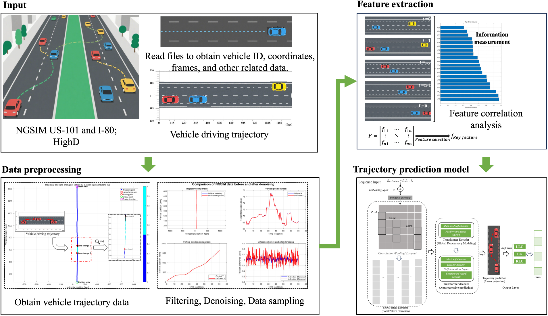
Figure 1: Overall framework for joint lane-changing intention recognition and vehicle trajectory prediction.

Historical target-vehicle states, surrounding-vehicle interactions, and road-related variables are first transformed into a unified feature sequence. MI scores are estimated exclusively from the training partition, and the highest-ranked variables form a compact input subset. The selected sequence is processed in parallel by a CNN branch for local motion variation and a Transformer branch for long-range temporal dependence. The fused representation is then supplied to an intention-classification head and a trajectory-regression head.

3.1 Problem Formulation

We begin by formalizing the joint intention recognition and trajectory prediction problem. Let H and F denote the number of observed historical time steps and future prediction steps, respectively. For a target vehicle indexed by r, its observed feature sequence is denoted by Xrobs∈RH×d, where d represents the number of selected input features. Specifically,

Xrobs=[xr,1Txr,2T⋮xr,HT]∈RH×d,(1)

where xr,t∈Rd denotes the feature vector of the target vehicle at time step t, containing the selected kinematic, interaction, and road-context variables.

The primary objective is to predict the future trajectory of the target vehicle. Let pr,t=[pr,tx,pr,ty]T∈R2 denote its two-dimensional position at time step t, where pr,tx and pr,ty represent the longitudinal and lateral coordinates, respectively. The future trajectory over the next F time steps is defined as

Yrfut=[pr,H+1,pr,H+2,…,pr,H+F]T∈RF×2.(2)

Concurrently, the model infers the driver’s maneuver intention, represented by the categorical variable cr∈{0,1,2}, corresponding to Lane Keeping (LK), Left Lane Changing (LLC), and Right Lane Changing (RLC), respectively.

Accordingly, a unified model fΘ maps the observed feature sequence to both the maneuver-intention probability vector and the future trajectory:

(π^r,Y^rfut)=fΘ(Xrobs).(3)

Here, Θ denotes the learnable parameters of the network, π^r is the estimated probability vector over the three maneuver classes, and Y^rfut denotes the predicted future trajectory. This joint formulation enables the model to learn shared representations for maneuver-intention recognition and geometric trajectory prediction.

3.2 Data Preprocessing

Data preprocessing is essential because raw vehicle trajectories extracted from videos often contain measurement noise, missing values, and inconsistent coordinate systems. In addition, the original datasets do not directly provide lane-changing intention labels suitable for supervised learning. Therefore, this study performs trajectory denoising, data standardization, and intention labeling before feature extraction and model training. Note that we first apply wavelet filtering (Section 3.2.1) and then perform standardization (Section 3.2.2), ensuring that noise removal is not affected by coordinate offsets.

3.2.1 Trajectory Filtering

Raw trajectories may contain missing observations and high-frequency measurement noise. Short internal gaps are filled by linear interpolation. NGSIM retains its original sampling rate of 10 Hz, whereas highD is resampled from 25 to 10 Hz. The resulting sampling interval, Δt=0.1 s, is used throughout the subsequent derivative calculations.

Let P=[p1,…,pN]T∈RN×2 denote a trajectory segment, where pt=[xt,yt]T. The discrete wavelet transform (DWT) is applied separately to the two coordinate sequences. The approximation coefficients preserve the dominant motion trend, whereas the detail coefficients are soft-thresholded to suppress measurement noise. The inverse discrete wavelet transform (IDWT) then reconstructs the denoised coordinates. Algorithm 1 gives the complete preprocessing procedure.

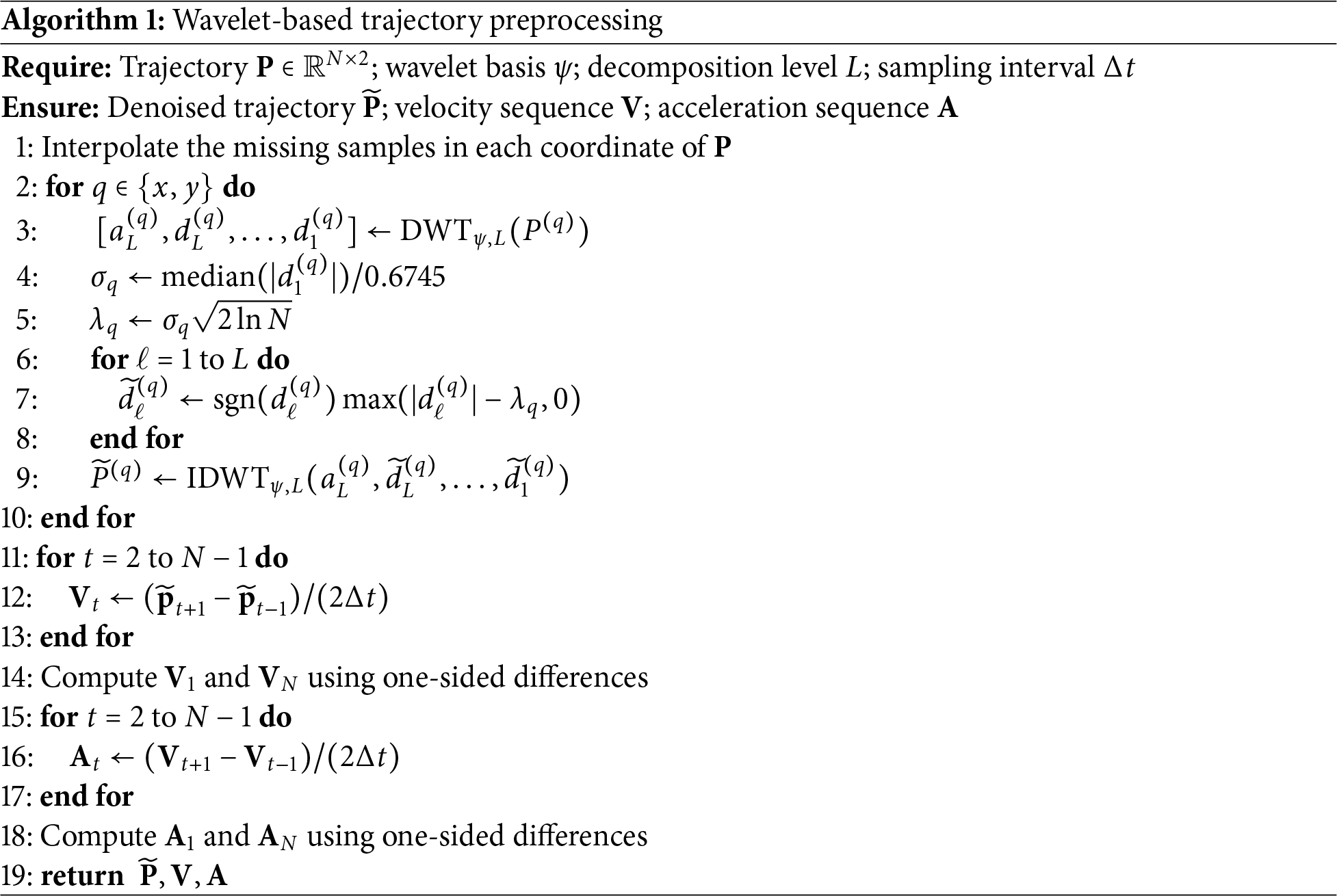
Fig. 2 illustrates a representative NGSIM trajectory before and after denoising.

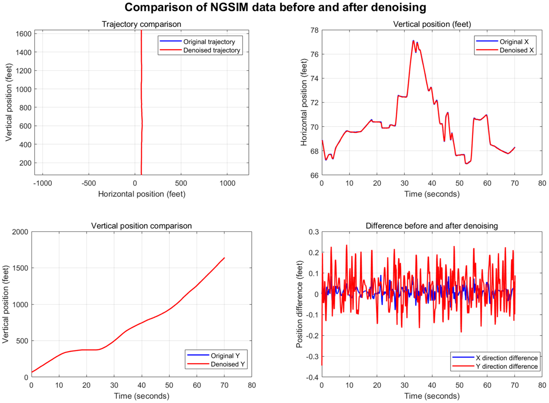
Figure 2: Representative lateral and longitudinal trajectory components before and after wavelet denoising for NGSIM Vehicle_ID 5.

The denoised trajectory preserves the dominant motion trend while reducing abrupt fluctuations that would otherwise be amplified when velocity and acceleration are computed.

3.2.2 Coordinate Standardization

All distance-related NGSIM fields are first converted from feet to meters using 1 ft=0.3048 m. The within-lane lateral coordinate is then calculated as

x~tng=0.3048LocalXt−(LaneIDt−1)dlane.(4)

where dlane is the lane width in meters. If lane-specific widths are available, the cumulative width of the lanes to the left of the current lane should replace (LaneIDt−1)dlane. This formulation keeps all terms in consistent metric units.

For highD, the lateral coordinate is expressed relative to the first observation in each extracted sequence:

x~thg=xt−x1,1≤t≤H.(5)

Before training, every continuous feature is standardized using the mean and standard deviation estimated from the training partition only. The same statistics are subsequently applied to the validation and test partitions.

3.2.3 Lane-Changing Intention Labeling

The original trajectory records do not directly provide the three intention labels required for supervised learning. Therefore, the lane-changing intention labels are generated from the lane identifier and lateral-motion information. As illustrated in Fig. 3, each lane-change maneuver is divided into three stages: preparation, lane-boundary crossing, and maneuver completion. A lane-boundary crossing is first detected when the lane identifier changes and the vehicle trajectory crosses the corresponding lane boundary. The crossing time is denoted by tc.

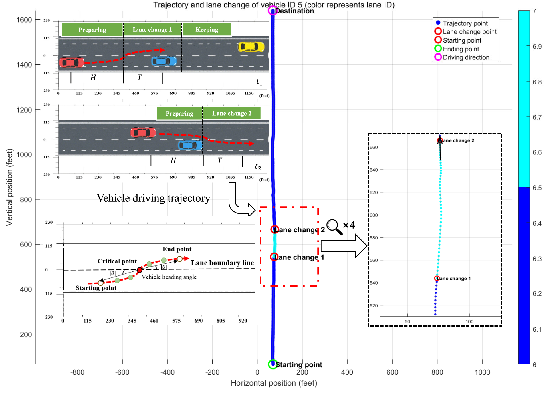
Figure 3: Definition of lane-change preparation, boundary crossing, and maneuver-completion stages.

To characterize the lateral motion more explicitly, the heading angle is computed using the quadrant-aware function

θt=atan2(xt−xt−1,yt−yt−1).(6)

Meanwhile, the lateral velocity is calculated as

vtlat=xt−xt−1Δt,(7)

where Δt=0.1 s is the sampling interval. Starting from tc, the trajectory is traced backward to determine the onset of the lane-change maneuver. Specifically, the maneuver onset is defined as the earliest time at which the absolute lateral velocity satisfies |vtlat|≥0.2 m/s for at least 0.5 s and the accumulated lateral displacement exceeds 0.3 m. These criteria are introduced to suppress short-term lateral fluctuations caused by trajectory noise or normal within-lane driving.

The maneuver-completion time is determined by tracing the trajectory forward from tc. A lane change is considered complete when the vehicle has entered the target lane, the absolute lateral velocity decreases below 0.2 m/s for at least 0.5 s, and the lateral distance between the vehicle and the centerline of the target lane is less than 0.3 m. The interval between the detected onset and completion times is labeled as Left Lane Changing (LLC) or Right Lane Changing (RLC) according to the direction of the lane-ID transition, whereas the remaining valid trajectory intervals are labeled as Lane Keeping (LK).

To distinguish intention prediction from state recognition, each sample is anchored before the actual lane-boundary crossing shown in Fig. 3. Specifically, the observation window is required to end at least 0.5 s before tc, while the corresponding lane-change event must occur within the subsequent prediction horizon. Therefore, the model predicts an upcoming maneuver rather than recognizing a lane change that has already occurred. Samples with ambiguous maneuver boundaries, discontinuous lane identifiers, insufficient trajectory duration, or incomplete lane-boundary crossings are excluded from the dataset.

3.3 Feature Extraction and Analysis

Lane-changing behavior is determined by the combined effects of the target vehicle’s own motion, neighboring-vehicle interactions, and lane-level road context. Therefore, feature extraction should not only describe the target vehicle trajectory, but also represent surrounding traffic constraints. In this study, the initial feature set is organized into target vehicle features, surrounding vehicle features, and road-related features. Mutual information is then used to screen the initial feature set and identify a compact subset that is most relevant to lane-changing intention.

3.3.1 Candidate-Feature Construction

The initial feature set consists of Target Vehicle Features (TVF), Surrounding Vehicle Features (SVF), and Road Features (RF). TVF describe the target vehicle’s lateral and longitudinal positions, velocities, accelerations, heading-related variables, and lane context. Let pt=[xt,yt]T denote the position vector. For interior time steps, the velocity and acceleration vectors are computed separately as

vt=pt+1−pt−12Δt,(8)

at=vt+1−vt−12Δt.(9)

One-sided differences are used at the sequence boundaries.

SVF characterize the interactions between the target vehicle and its surrounding vehicles. As illustrated in Fig. 4, six relative positions are considered: front, rear, left-front, left-rear, right-front, and right-rear. To provide a compact representation of the interaction features, the motion state of vehicle j is defined as stj=[(ptj)T,(vtj)T,(atj)T]T. The relative state of surrounding vehicle i with respect to the target vehicle r is then expressed as

Δsti=sti−str.(10)

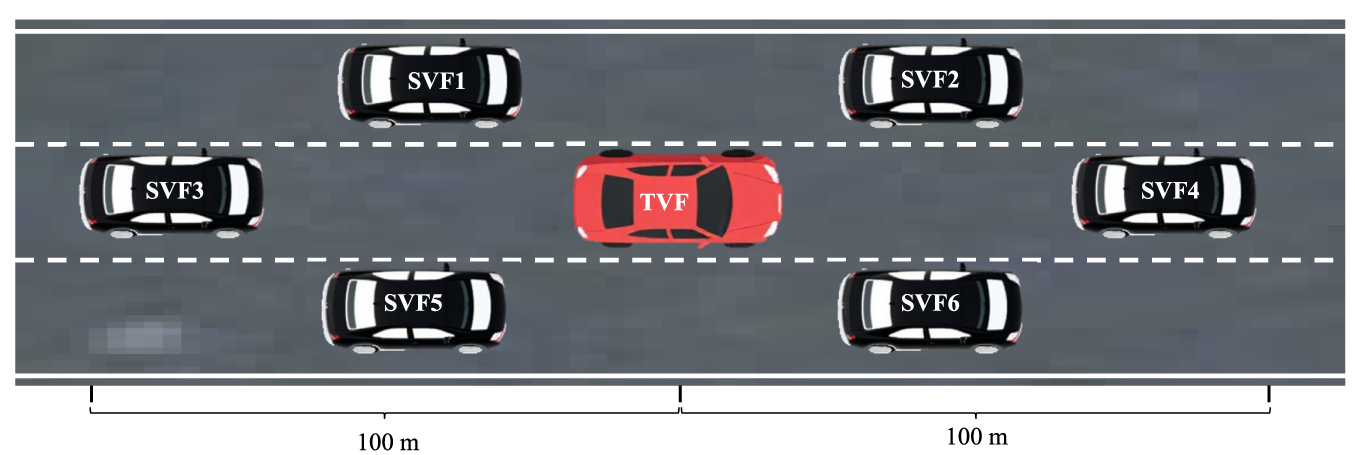
Figure 4: Six surrounding-vehicle positions considered relative to the target vehicle.

When any of the six surrounding positions shown in Fig. 4 is unoccupied, a virtual vehicle is introduced to maintain a fixed input dimension. Its lateral offset is determined according to the corresponding lane position, while its longitudinal distance is assigned a finite maximum-range value Dmax. Its velocity and acceleration are set equal to those of the target vehicle. Consequently, the relative velocity and acceleration of a missing neighbor are zero, whereas its large longitudinal separation minimizes its interaction effect. In the reported implementation, Dmax=1000 m. RF include the current lane identifier, availability of adjacent lanes, lane width, and selected headway or interaction variables. In total, 40 candidate variables are constructed and denoted by ℱ={F1,…,F40}.

3.3.2 Mutual-Information-Guided Feature Selection

Mutual information (MI) measures the statistical dependence between a candidate feature Fi and the maneuver label C. Unlike Pearson correlation, MI is not restricted to linear relationships. For discrete variables, it is defined as

I(Fi;C)=∑f∈𝒟i∑c∈𝒞pFi,C(f,c)log⁡pFi,C(f,c)pFi(f)pC(c),(11)

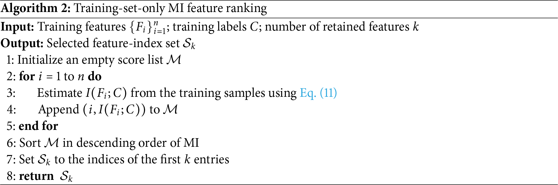
where continuous variables are discretized using a fixed rule estimated solely from the training partition before the empirical probabilities in Eq. (11) are calculated. The same discretization rule is applied to all candidate features. Algorithm 2 summarizes the MI-based ranking procedure, while Fig. 5 illustrates the overall training-set-only feature-selection process and the subsequent transfer of the selected feature indices to the validation and test partitions.

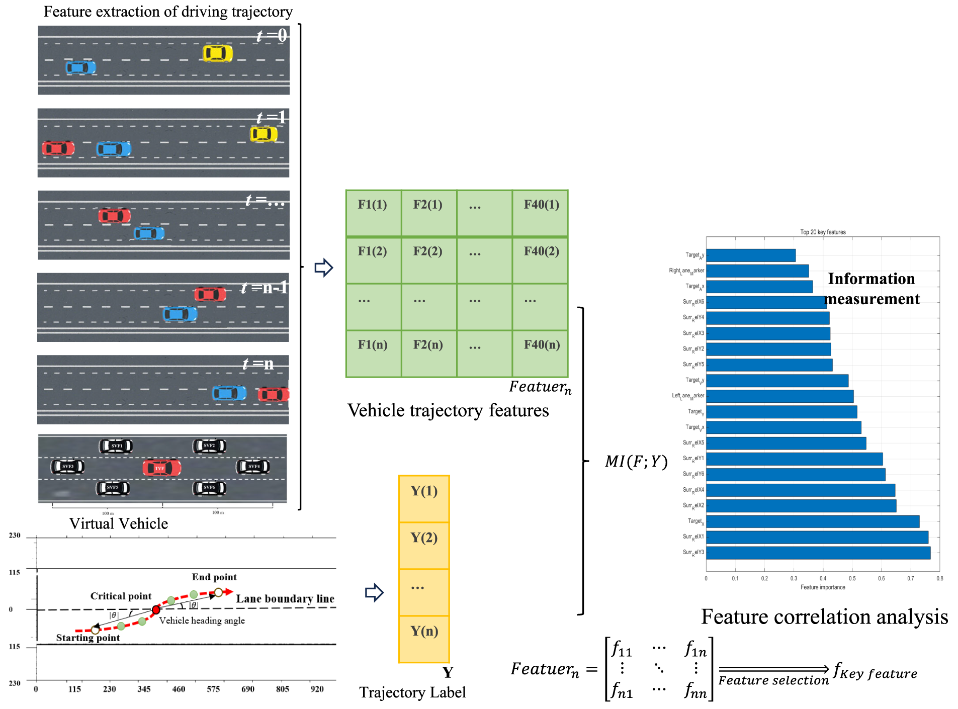
Figure 5: Training-set-only feature ranking and transfer of the selected indices to validation and test partitions.

As shown in Fig. 5, MI ranking is performed only after the vehicle-wise training–validation–test split. Therefore, neither validation nor test labels are involved in feature ranking or feature selection, thereby preventing information leakage. The MI ranking is independently estimated for the NGSIM and highD datasets because their acquisition systems and feature distributions differ.

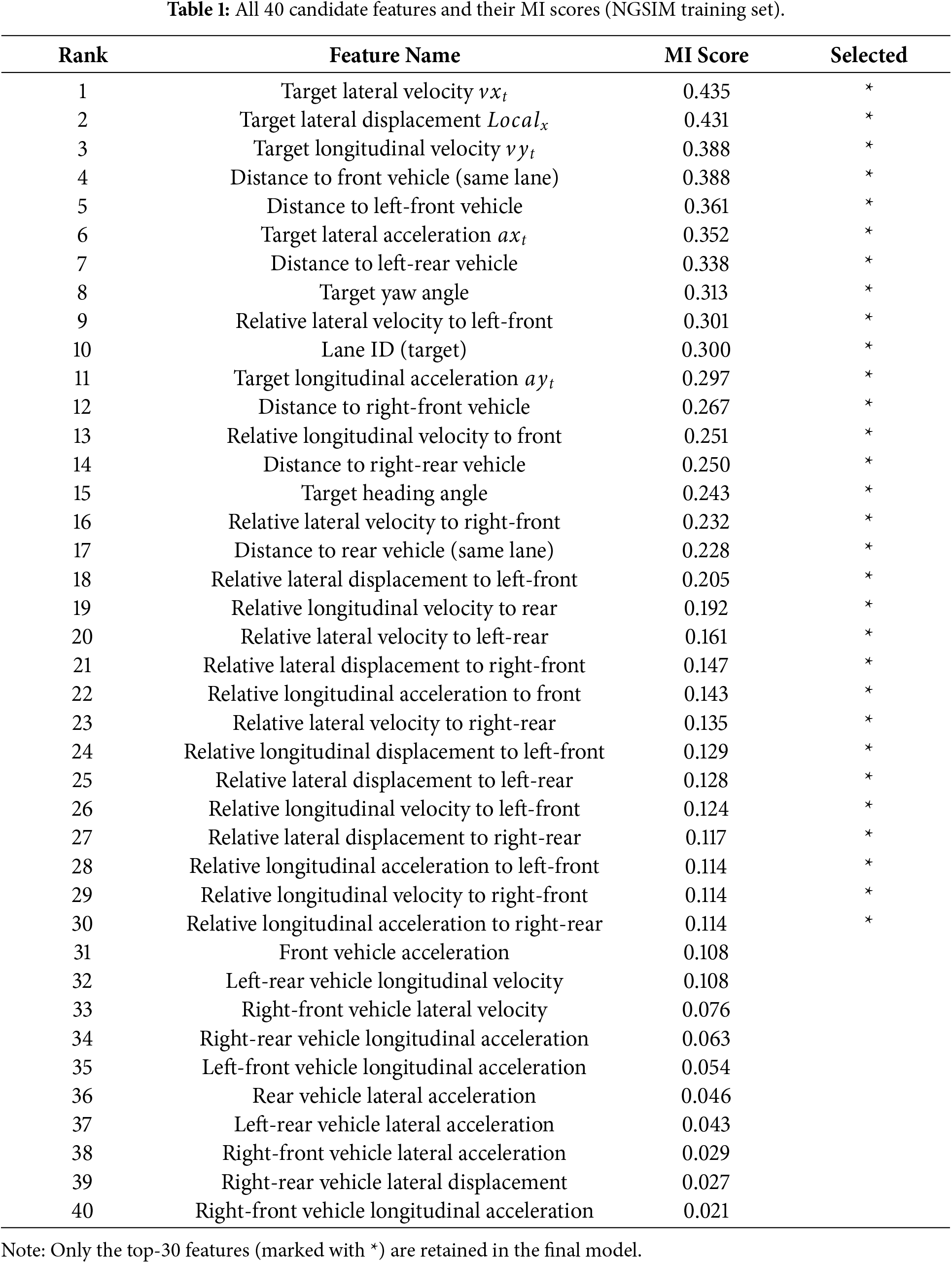
3.3.3 Complete Feature List and MI Ranking

Table 1 reports the NGSIM training-set ranking as an illustrative example, with the 30 retained variables marked by an asterisk. For the highD dataset, MI ranking is independently performed using its own training partition following the same procedure, and the top 30 features are retained for subsequent model training.

3.4 Hybrid CNN–Transformer Multi-Task Network

The selected historical sequence Xobs∈RH×d is supplied to two parallel temporal encoders. The CNN branch emphasizes short-duration motion changes, such as lateral drift, velocity fluctuation, and acceleration variation. The Transformer branch models dependencies across the complete observation window and captures longer-term maneuver evolution. Their outputs are fused and shared by an intention-classification head and a trajectory-regression head. Therefore, the two tasks are not trained as independent post-processing modules; instead, both losses update the shared CNN–Transformer representation during backpropagation.

In Fig. 6, batch normalization (BN), the rectified linear unit (ReLU), and the fully connected (FC) layer denote the normalization operation, activation function, and dense projection operation, respectively.

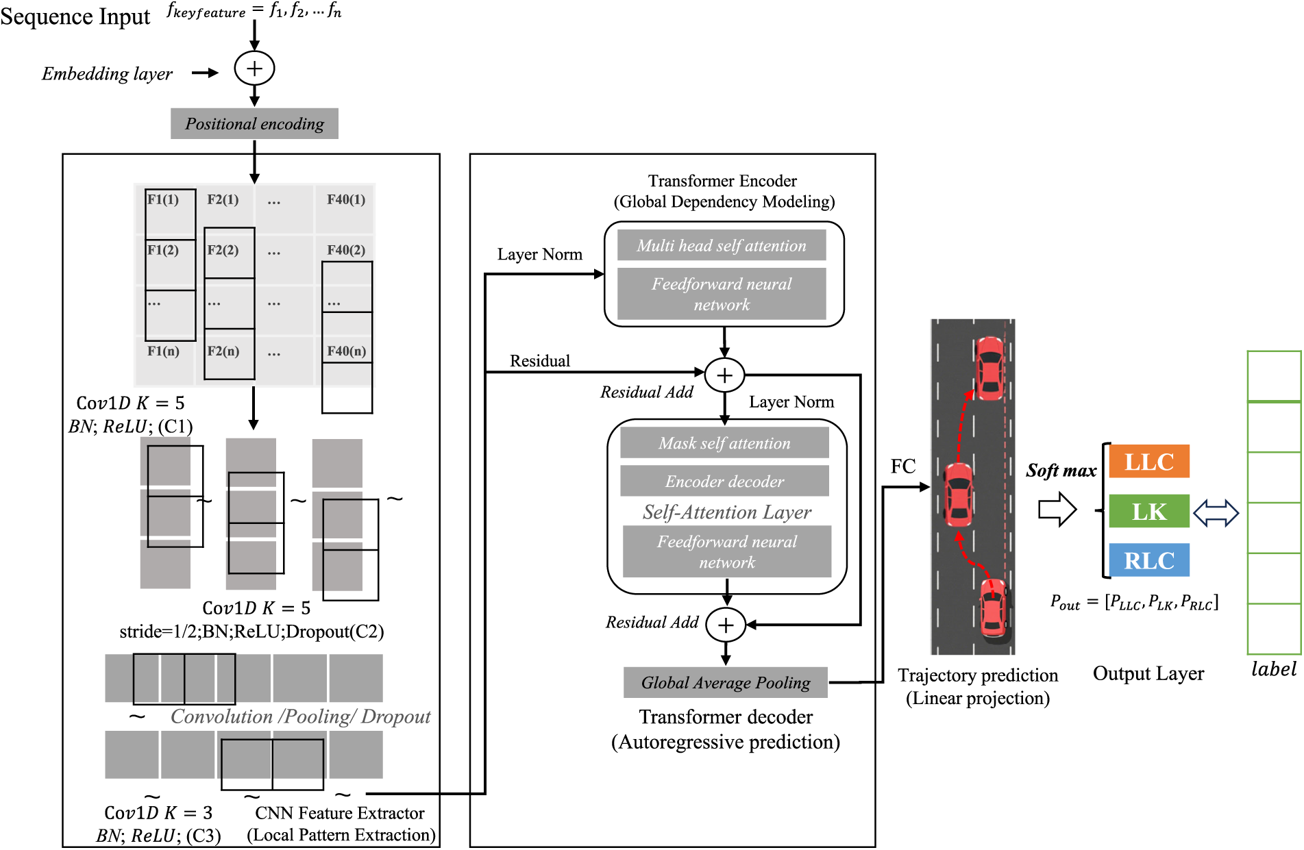
Figure 6: Detailed structure of the hybrid CNN–Transformer multi-task network. The selected historical sequence is processed by parallel local and global temporal encoders, followed by feature fusion, an intention-classification head, and a trajectory-regression head.

3.4.1 Local Temporal Encoding with the CNN Branch

The CNN branch uses one-dimensional convolutions along the temporal axis. Starting from the input sequence Hcnn(0)=Xobs, the output of each of the ℓ-th convolutional block is computed. This process can be formalized as:

Hcnn(ℓ)=ReLU(BN(Conv1Dℓ⁡(Hcnn(ℓ−1)))),ℓ=1,…,Lcnn.(12)

Here, Conv1Dℓ represents the 1D convolutional operation, BN is batch normalization, and ReLU is the activation function. The convolutional receptive field aggregates neighboring time steps and is therefore suitable for detecting short-term precursor patterns before a lane change. Following the convolutional blocks, a temporal pooling operation aggregates the features over the time dimension, producing a fixed-length, compact local representation vector vcnn:

vcnn=TemporalPool⁡(Hcnn(Lcnn)).(13)

This vector encapsulates the key short-term motion patterns identified by the CNN.

3.4.2 Global Temporal Encoding with the Transformer Branch

In parallel, the input sequence is first projected into an embedding space and combined with positional encoding to create the initial representation for the Transformer encoder, denoted as Z(0). This process is defined as:

Z(0)=XobsWe+be+P,(14)

where We and be are trainable projection parameters and P denotes the positional encoding. The Transformer branch then processes this sequence through Ltr identical blocks. The core of each block is the multi-head self-attention mechanism, which allows each time step to directly attend to all others, thereby capturing long-range dependencies. The operations within the m-th Transformer block can be described as:

Z~(m)=LN[Z(m−1)+MHA(Z(m−1))],(15)

Z(m)=LN[Z~(m)+FFN(Z~(m))],m=1,…,Ltr.(16)

Here, MHA denotes the multi-head attention function, FFN is a position-wise feed-forward network, and LN represents layer normalization. This architecture models global temporal dependencies without the sequential constraints of RNNs. Finally, a temporal pooling operation aggregates the output of the final Transformer block Z(Ltr) into a single global representation vector vtr:

vtr=TemporalPool⁡(Z(Ltr)).(17)

3.4.3 Feature Fusion and Task-Specific Prediction Heads

The local representation vcnn from the CNN and the global representation vtr from the Transformer are complementary. They are fused by a simple concatenation operation to form a comprehensive shared feature vector:

vfuse=[vcnn;vtr].(18)

This fused vector vfuse is the input to two task-specific heads. The intention-classification head maps this vector to three class scores (logits), which are then passed through a softmax function to produce the final class probabilities π^:

π^=softmax(gcls(vfuse)),(19)

where gcls(⋅) is a linear projection layer. The trajectory-regression head, which is another linear projection layer greg(⋅), outputs 2F values representing the x and y coordinates for each of the F future time steps. These values are then reshaped to form the final predicted trajectory matrix Y^fut:

Y^fut=reshape(greg(vfuse),F,2).(20)

Sharing the fused representation enables maneuver semantics to constrain the learned motion representation, while geometric trajectory supervision prevents the shared encoder from focusing only on classification-related cues.

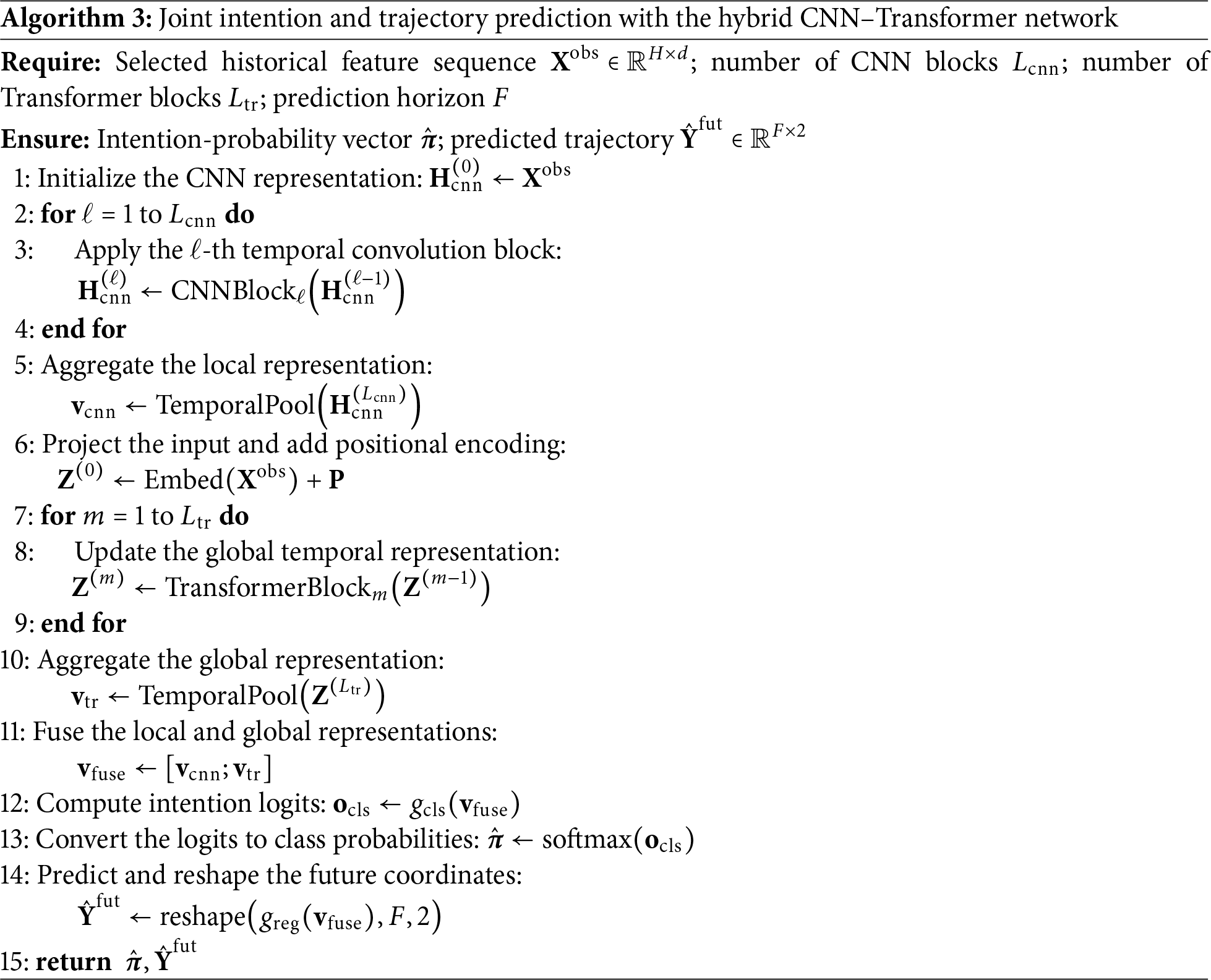
Algorithm 3 presents the complete forward-propagation procedure for one selected historical sequence.

3.4.4 Joint Multi-Task Optimization

For a mini-batch containing B samples, the intention-classification loss is the standard cross-entropy loss:

ℒcls=−1B∑b=1Blog⁡π^b,cb,(21)

where cb is the ground-truth intention class of sample b. The trajectory-regression loss is the mean squared error (MSE) between the predicted and ground-truth future positions:

ℒreg=1BF∑b=1B∑t=1F‖y^b,t−yb,t‖22.(22)

The total multi-task objective is a weighted sum of the two losses:

ℒ=ℒcls+λℒreg,(23)

where λ controls the contribution of trajectory regression. The reported experiments use λ=0.1. During training, gradients from both loss terms are propagated through the task-specific heads, the fusion layer, and the two temporal encoders. This joint update mechanism is the central connection between intention recognition and trajectory prediction in the proposed framework.

4  Experimental Analysis

This section introduces the datasets and their harmonization, presents the experimental configuration, and evaluates the proposed method on NGSIM and highD. The experiments examine four questions: (1) how the number of retained features affects performance; (2) how observation and prediction horizons influence trajectory error; (3) whether local–global feature fusion improves over representative baselines; and (4) how preprocessing and model components contribute to the final results. All models are trained in MATLAB 2024b on a workstation equipped with an Intel® Core i9-11900H central processing unit (CPU) and an NVIDIA® GeForce RTX 4060 graphics processing unit (GPU).

4.1 Datasets and Unified Visual Presentation

The experiments use the public Next Generation Simulation (NGSIM) vehicle-trajectory dataset and the highD naturalistic highway trajectory dataset. NGSIM was recorded by fixed cameras at 10 Hz and contains trajectories from the U.S. Highway 101 (US-101) and Interstate 80 (I-80) road sections. The US-101 and I-80 subsets represent congested multilane freeway traffic under different road layouts and traffic conditions. The highD dataset was collected by aerial drones on German highways at 25 Hz and contains trajectories of approximately 110,000 vehicles, including more than 5,000 complete lane-change maneuvers. Compared with highD, NGSIM contains denser traffic and noisier position measurements, which enables the model to be evaluated under different acquisition conditions.

To improve visual consistency, the three dataset scenes are presented using the same panel dimensions, border style, typography, and annotation layout in Fig. 7. Each panel identifies the dataset subset, acquisition platform, and original sampling frequency. The displayed trajectory segments were cropped from the original dataset visualizations and aligned to a comparable road-centered view, with consistent panel dimensions, border style, typography, and annotation layout applied across all three datasets.

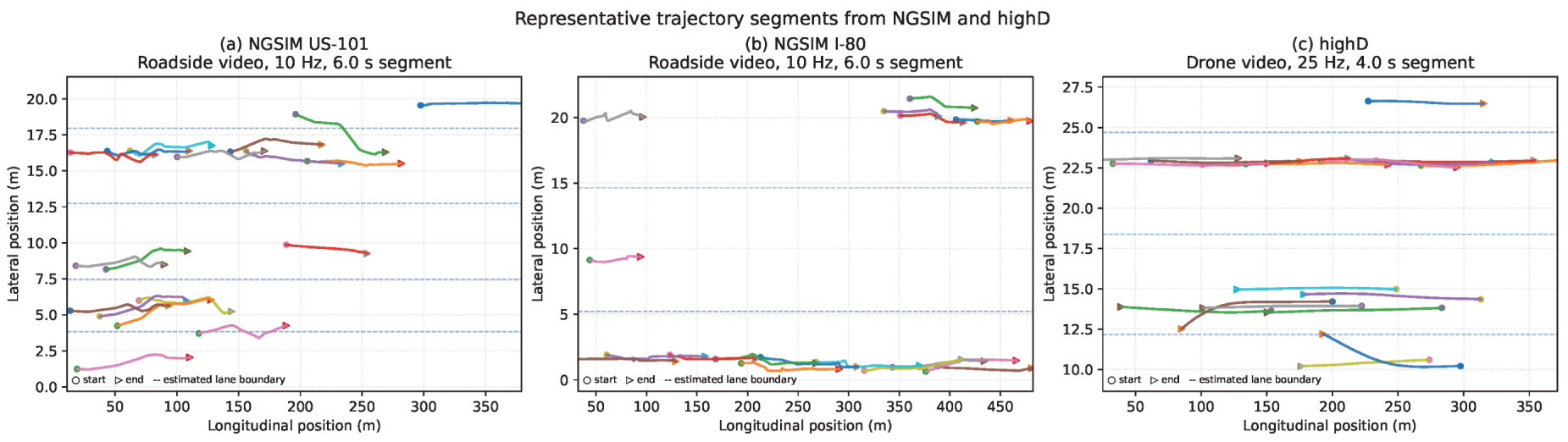
Figure 7: Representative trajectory segments from the NGSIM US-101, NGSIM I-80, and highD datasets.

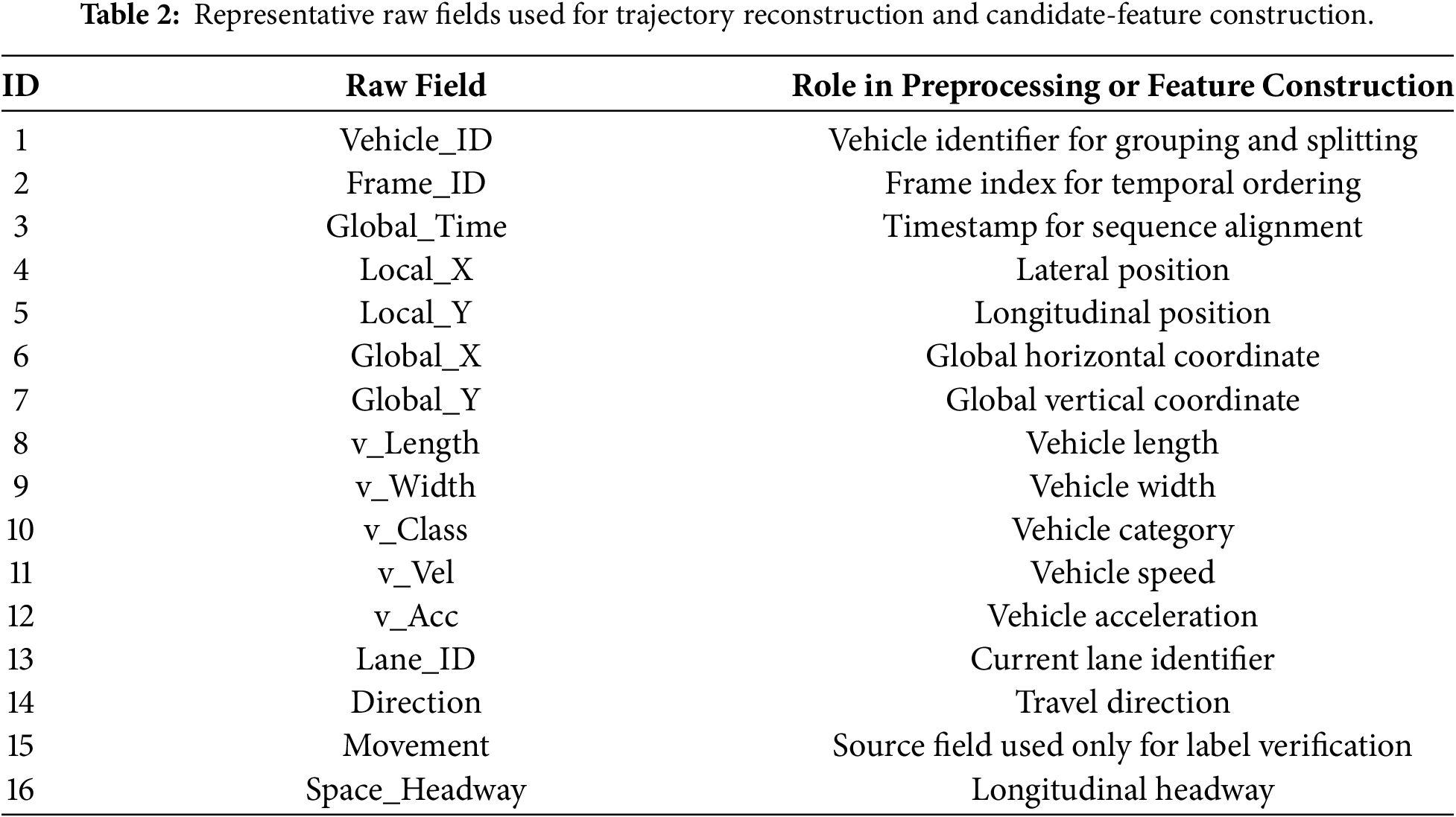
Table 2 lists representative raw fields used for trajectory reconstruction and candidate-feature construction. Identification fields and acquisition metadata, such as Vehicle_ID, Frame_ID, and Global_Time, are used only for trajectory reconstruction and vehicle-wise data partitioning; they are not supplied to the prediction network. The Movement field is used only to verify the maneuver labels generated from the lane-transition and lateral-motion criteria described above, and is likewise excluded from the model input to prevent label leakage.

The highD dataset records distances in meters, whereas NGSIM uses feet. Therefore, all distance-related variables in NGSIM are converted to meters before feature computation. NGSIM retains its original sampling frequency of 10 Hz, while highD is resampled from 25 to 10 Hz so that both datasets use a common sampling interval of Δt=0.1 s. MI estimation and feature ranking are performed independently using only the training partition of each dataset. Because lane-keeping samples account for approximately 80% of the extracted sequences, class-wise metrics and macro-averaged F1 scores are reported together with overall accuracy.

4.2 Experimental Details

For both datasets, models are trained using different numbers of selected key features (k∈{10,20,25,30,35,40}). The experimental results are evaluated using trajectory prediction metrics and intention classification metrics. Unless otherwise stated, the historical observation horizon is set to 5 s and the future prediction horizon is set to 3 s.

4.2.1 Training Parameter Configuration

Each model is trained for 100 epochs with a batch size of 1,024. The Adam optimizer is adopted with an initial learning rate of 0.001 and a weight decay of 0.0001. For each dataset, we split the data by vehicle ID to avoid any temporal overlap between training and testing sets. 70% of vehicles are used for training, 15% for validation, and 15% for testing. All trajectory segments from the same vehicle belong exclusively to one split. This vehicle-wise partitioning prevents over-optimistic performance estimates caused by correlated samples. All in-house baseline models use the same vehicle-wise partitions, observation windows, prediction horizons, and evaluation code.

The complete CNN–Transformer model contains 2.3 million trainable parameters and requires approximately 1.8 billion floating-point operations (1.8 GFLOPs) for one forward pass. On the stated NVIDIA GeForce RTX 4060 GPU, the measured inference time is 12.5 ms per sample and the peak GPU memory consumption is approximately 1.2 gigabytes (GB). These measurements characterize network-level computational efficiency under the reported experimental platform; they do not include the latency of sensing, trajectory preprocessing, host–device data transfer, or downstream planning.

4.2.2 Evaluation Metrics for Intention and Trajectory Prediction

For trajectory prediction, let yn,t and y^n,t denote the ground-truth and predicted two-dimensional coordinates of sample n at future step t, respectively. The Final Displacement Error (FDE) measures the Euclidean distance between the predicted and ground-truth positions at the final prediction step. For the n-th sample, it is defined as

FDEn=‖y^n,F−yn,F‖2.(24)

The mean FDE over all N test samples is computed as

FDE=1N∑n=1N‖y^n,F−yn,F‖2,(25)

where N denotes the number of test samples and F denotes the final prediction step. In addition, coordinate-wise root mean square error (RMSE) and mean absolute error (MAE) are reported to evaluate trajectory-prediction accuracy in the lateral and longitudinal directions. Mean absolute percentage error (MAPE) is used only in the feature-count sensitivity analysis and is interpreted cautiously when the reference coordinate approaches zero. For intention recognition, the evaluation metrics are calculated independently for each class under a one-vs.-rest protocol. Specifically, Precisionc=TPc/(TPc+FPc), Recallc=TPc/(TPc+FNc), and F1c=2Precisionc⁡Recallc⁡/(Precisionc+Recallc). Overall accuracy is defined as the proportion of correctly classified samples, while macro-F1 is computed as the arithmetic mean of the class-wise F1-scores. Both metrics are reported to provide a balanced evaluation under class-imbalanced conditions.

4.3 Feature-Count and Horizon Sensitivity

We evaluate the trajectory prediction performance by sequentially varying the number of input features. The model is designed to utilize 5 s of historical trajectory data to predict the subsequent 3-s trajectory, along with the associated driving intention. Experiments are conducted on the NGSIM dataset, and the results are summarized in Table 3.

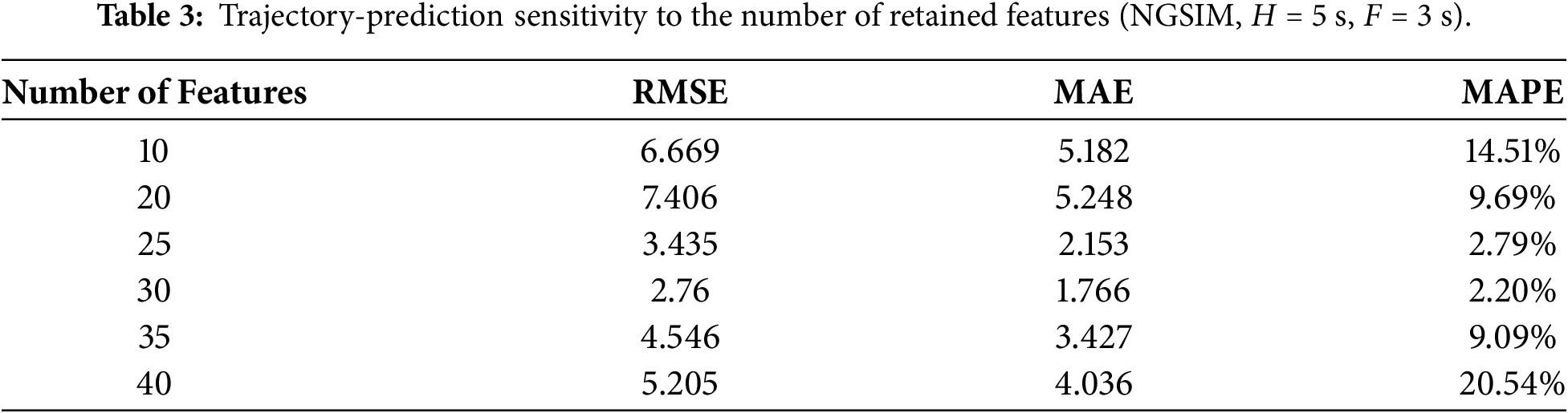
As shown in Table 3, the model achieves the lowest RMSE and MAE when 30 features are selected. When too few features are retained, the input representation may lose important interaction information. Conversely, when too many features are included, redundant or weakly relevant variables may introduce noise and reduce generalization. Therefore, 30 key features are used in the subsequent experiments.

To evaluate the influence of different historical observation and future prediction horizons on trajectory prediction performance, we considered five observation horizons (H∈{2,3,4,5,6} s) and five future prediction horizons (F∈{1,2,3,4,5} s). All combinations of H and F were evaluated, and the experimental results are presented in Table 4.

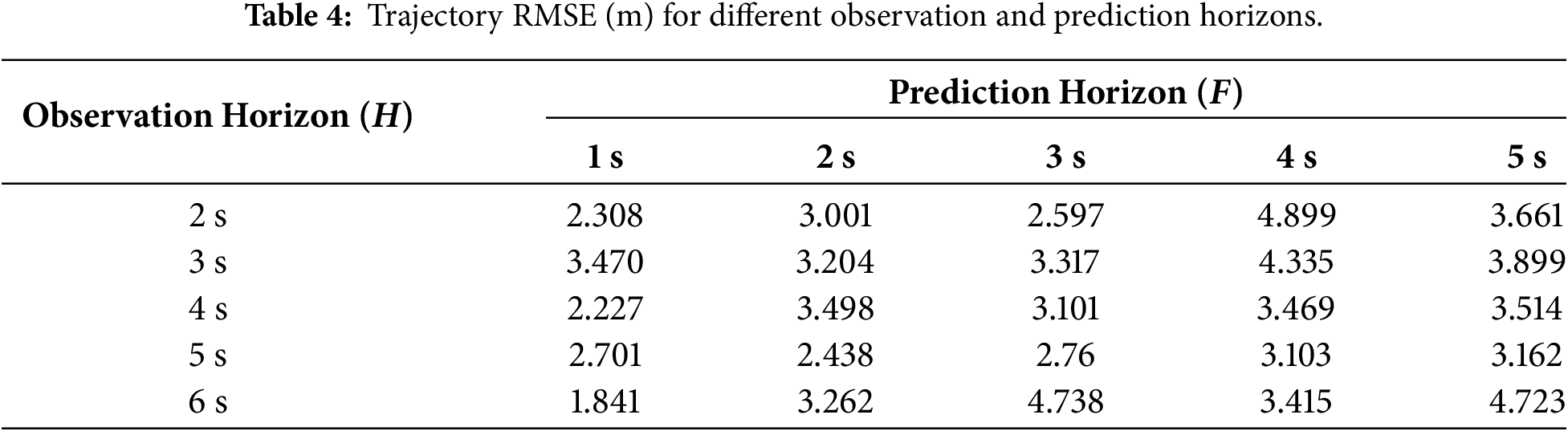
Table 4 shows that the error does not vary monotonically with observation length, indicating that additional history is not uniformly beneficial. The setting H=5 s and F=3 s is used as the principal evaluation scenario because it provides a sufficiently long observation window while retaining a practically relevant 3-s forecast. This setting should be described as a predefined evaluation protocol rather than the unique numerical optimum. The corresponding intention-recognition results are reported in Table 5.

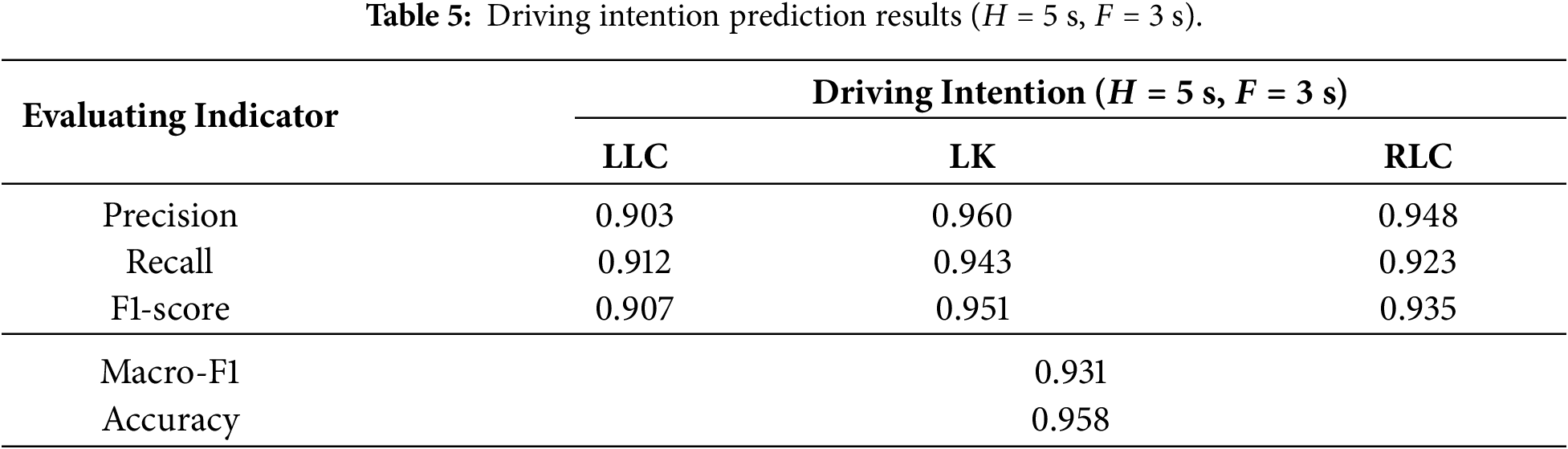
The results indicate that the proposed method achieves stable performance for all three intention classes. In particular, the model maintains competitive precision and recall for LLC and RLC, which are more safety-critical than lane keeping in autonomous driving applications.

4.4 Detailed Trajectory-Prediction Analysis

To provide a more detailed evaluation of trajectory-prediction performance, we report the FDE, lateral RMSE, and longitudinal RMSE on the NGSIM dataset under H=5 s and F=3 s. The results are presented in Table 6.

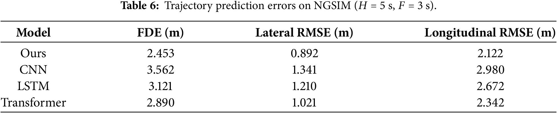
As shown in Table 6, the proposed method achieves the lowest FDE as well as the lowest lateral and longitudinal RMSE values among the evaluated in-house baselines. These results indicate that the proposed model provides more accurate trajectory estimates in both lateral and longitudinal directions. Because lateral and longitudinal motion have different physical ranges, however, the magnitudes of their RMSE values should not be directly interpreted as indicators of relative modeling difficulty. In addition, the increase in displacement error over longer prediction horizons is consistent with the accumulation of motion uncertainty. Ablation experiments were conducted on the NGSIM dataset with H=5 s and F=3 s to evaluate the contribution of the major components. Six configurations were considered. The variant without MI-based feature selection retains all 40 candidate features while keeping the remaining components of the complete model unchanged. This configuration is equivalent to the 40-feature setting reported in Table 3, since retaining all 40 candidate features effectively removes the feature-screening effect of MI. The variant without wavelet preprocessing omits trajectory denoising. A CNN-only model without MI was constructed by using all 40 candidate features and removing the Transformer branch. Two additional variants retained MI-based feature selection but used either the Transformer branch alone or the CNN branch alone. These variants were compared with the complete model incorporating MI-guided feature selection, wavelet preprocessing, and CNN–Transformer fusion. The complete model achieved an intention-recognition accuracy of 95.81% and a trajectory RMSE of 2.76 m. When MI-based feature selection was removed and all 40 candidate features were retained, the accuracy decreased to 91.23% and the trajectory RMSE increased to 5.205 m, consistent with the 40-feature result reported in Table 3. Removing wavelet preprocessing resulted in an accuracy of 93.10% and an RMSE of 3.02 m. The CNN-only model without MI obtained an accuracy of 89.76% and an RMSE of 3.87 m. When MI-based feature selection was introduced into the CNN-only architecture, the accuracy increased to 93.52% and the RMSE decreased to 3.33 m, indicating that feature selection improves both intention recognition and trajectory regression. The Transformer-only model achieved an accuracy of 92.45% and an RMSE of 3.21 m, which remained inferior to the complete model. Overall, these results indicate that MI-guided feature selection, wavelet-based trajectory preprocessing, and complementary local-global temporal modeling contribute to the final prediction performance. In particular, the comparison between the complete model and the all-feature configuration demonstrates that retaining all candidate variables does not necessarily improve prediction accuracy; instead, irrelevant or redundant variables may introduce additional noise into the trajectory-regression process. The comparison between the two CNN variants further isolates the contribution of feature selection from that of the Transformer branch. Nevertheless, classification-only and regression-only variants would be required to further quantify the independent contribution of multi-task optimization.

4.5 Comparison with In-House Baselines

To compare the performance of different models in vehicle trajectory prediction, we evaluated several architectures, including a CNN, LSTM, CNN-LSTM, Transformer, and spatiotemporal-attention LSTM (STA-LSTM) [29,30]. The models were compared based on their predictions of trajectory coordinates (x and y), with the results illustrated in Fig. 8.

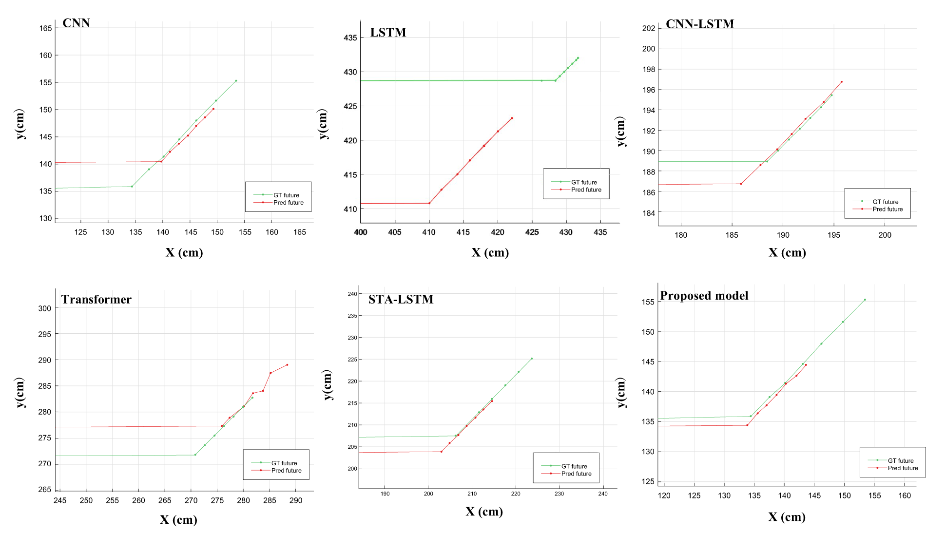
Figure 8: Comparison of trajectory prediction results.

As shown in Fig. 8, the predicted trajectories generated by the proposed model are closely aligned with the ground-truth trajectories, especially during lane-changing-related lateral motion. This indicates that the selected features and CNN–Transformer fusion can effectively represent both local kinematic variation and longer-term motion tendency. Furthermore, we employ a confusion matrix to visualize the classification results of the three driving intention categories, as shown in Fig. 9.

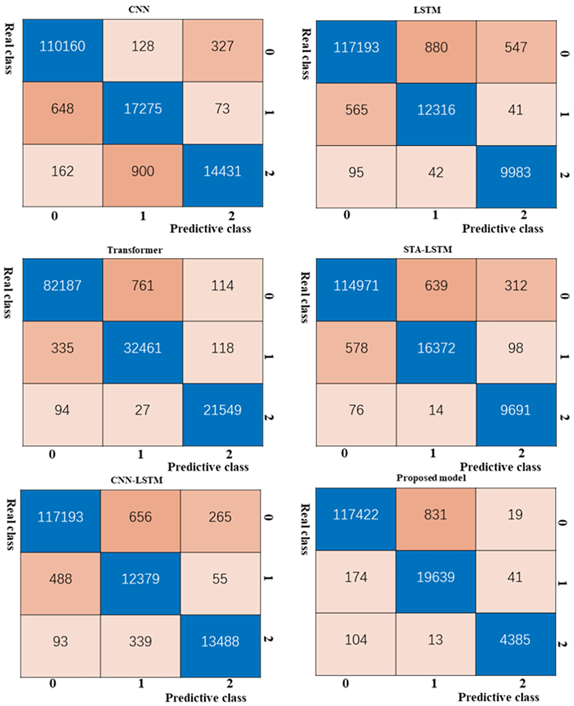
Figure 9: Confusion matrix of driving intention prediction results.

As indicated in the figure, label 0 corresponds to LK, 1 to LLC, and 2 to RLC. Vehicle intention recognition constitutes a class-imbalanced problem, as the majority of samples belong to the lane-keeping category. However, in practical applications, lane-changing scenarios cannot be overlooked due to their critical impact on safety. The confusion matrix shows that most samples are correctly classified, and the proposed method reduces confusion between lane keeping and lane-changing categories. This is important because misclassifying an imminent lane change as lane keeping may lead to delayed decision-making in autonomous driving systems.

4.6 Intention-Recognition Results across Prediction Horizons

To further evaluate intention prediction performance, the proposed method is compared with CNN, LSTM, and Transformer baselines on NGSIM and highD. The results are reported under three prediction horizons (F=1 s, F=2 s, and F=3 s). Tables 7 and 8 summarize the class-wise precision, recall, F1-score, and overall accuracy for NGSIM and highD, respectively.

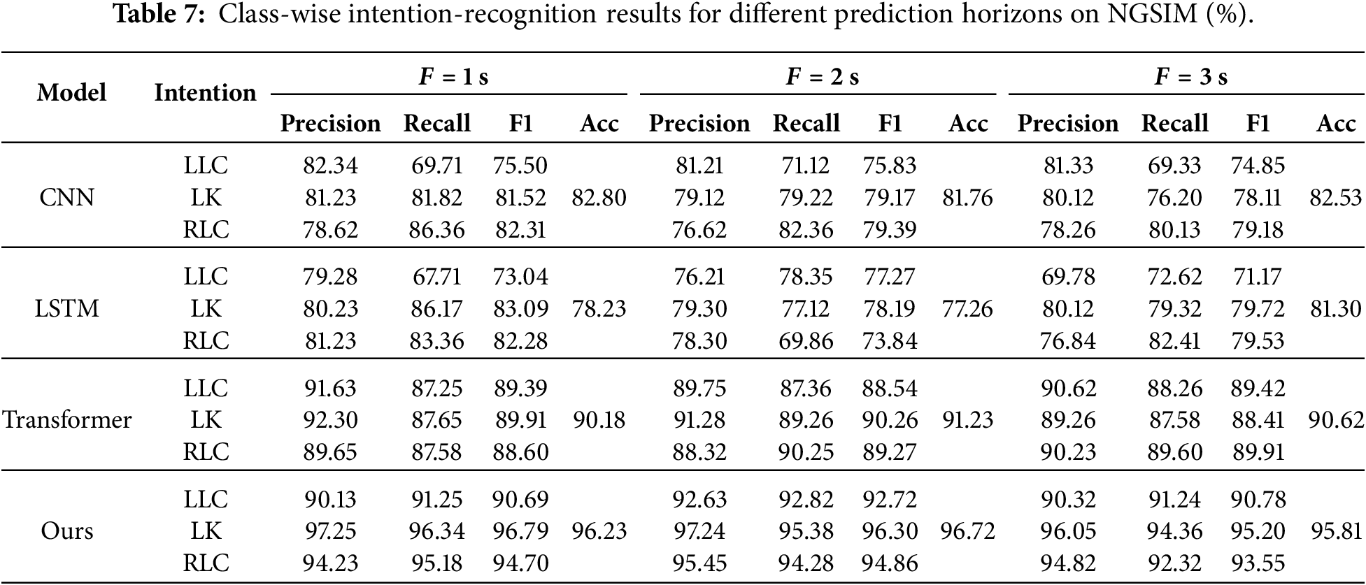
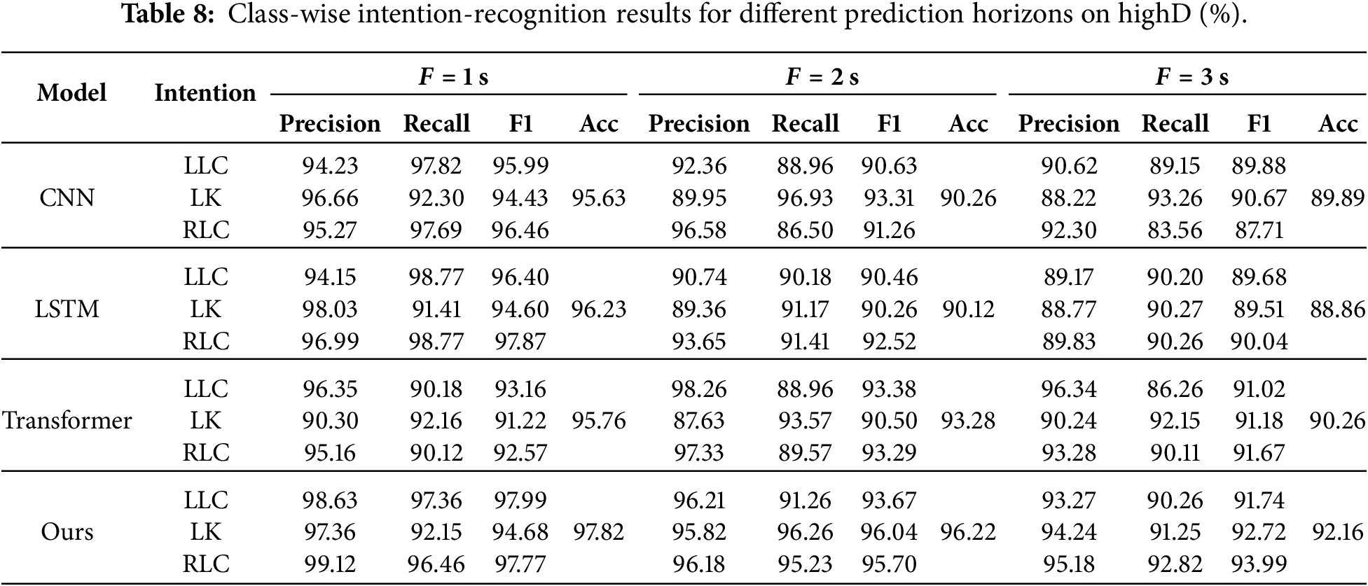
Based on Tables 7 and 8, the proposed method generally achieves higher overall accuracy than the baseline models on both datasets. The improvement is more evident for longer prediction horizons, where local motion cues alone are insufficient and global temporal dependencies become more important. Compared with CNN, the proposed method benefits from self-attention-based long-range dependency modeling. Compared with LSTM, it avoids purely sequential information propagation and supports more efficient parallel temporal representation. Compared with the standalone Transformer, the CNN branch provides local motion features that help identify early lane-changing cues. These results confirm the complementary role of mutual-information-guided feature selection and CNN–Transformer fusion.

5  Conclusion

This paper presented a joint lane-changing intention and vehicle trajectory prediction framework based on MI-guided feature selection and hybrid CNN–Transformer encoding. The method constructs target-vehicle, surrounding-vehicle, and road-context variables from denoised and standardized trajectories. MI ranking is performed only on the training partition to retain a compact feature subset. The selected sequence is then processed by complementary convolutional and self-attention branches, and the fused representation is optimized through intention-classification and trajectory-regression objectives.

Experiments on NGSIM and highD indicate that retaining 30 ranked features provides a favorable balance between input compactness and predictive performance. With 5 s of observation and a 3-s prediction horizon, the model achieves intention-recognition accuracies of 95.81% and 92.16% on NGSIM and highD, respectively. The in-house baseline and ablation results support the contributions of feature selection, trajectory denoising, and local–global temporal representation. The implementation measurements reported with the experimental settings indicate that the network can perform low-latency inference on the stated desktop GPU.

Several limitations remain. First, the benefit of multi-task learning should be quantified through classification-only and regression-only variants and through sensitivity analysis of the loss weight. Second, repeated experiments and statistical significance analysis are required to characterize variability across random initialization and data partitioning. Third, cross-road and cross-dataset transfer experiments are needed to evaluate generalization under domain shift. Future work will also investigate uncertainty-aware multimodal trajectory prediction, causal or redundancy-aware feature selection, and end-to-end deployment tests on embedded automotive hardware.

Acknowledgement: Not applicable.

Funding Statement: This work was supported by the National Natural Science Foundation of China under Grant (62341118,62503241), in part by the Natural Science Foundation of Jiangsu Province of China under Grant (BK20250664), and by the Talent Recruitment Foundation of Huaiyin Institute of Technology (HYIT) under Grant (Z301B25508).

Author Contributions: The authors confirm contribution to the paper as follows: study conception and design: Huaran Zhou, Gaoteng Yuan and Ping Qiu; data processing: Gaoteng Yuan and Ping Qiu; analysis and interpretation of results: Gaoteng Yuan; draft manuscript preparation: Huaran Zhou, Gaoteng Yuan and Ping Qiu; review and editing: Ping Qiu; funding acquisition: Ping Qiu. All authors reviewed and approved the final version of the manuscript.

Availability of Data and Materials: The Next Generation Simulation (NGSIM) Open Data used in this study are publicly available from the U.S. Department of Transportation, Federal Highway Administration, at https://ops.fhwa.dot.gov/trafficanalysistools/ngsim.htm. The highD dataset is publicly available from levelXdata at https://levelxdata.com/highd-dataset/. No new dataset was generated in this study.

Ethics Approval: Not applicable.

Conflicts of Interest: The authors declare no conflicts of interest.

References

1. Gao K, Li X, Chen B, Hu L, Liu J, Du R, et al. Dual transformer based prediction for lane change intentions and trajectories in mixed traffic environment. IEEE Trans Intell Transp Syst. 2023;24(6):6203–16. doi:10.1109/tits.2023.3248842. [Google Scholar] [CrossRef]

2. Mozaffari S, Arnold E, Dianati M, Fallah S. Early lane change prediction for automated driving systems using multi-task attention-based convolutional neural networks. IEEE Trans Intell Veh. 2022;7(3):758–70. doi:10.1109/tiv.2022.3161785. [Google Scholar] [CrossRef]

3. Sarker A, Shen H, Rahman M, Chowdhury M, Dey K, Li F, et al. A review of sensing and communication, human factors, and controller aspects for information-aware connected and automated vehicles. IEEE Trans Intell Transp Syst. 2020;21(1):7–29. doi:10.1109/tits.2019.2892399. [Google Scholar] [CrossRef]

4. Wang Y, Jiang J, Li S, Li R, Xu S, Wang J, et al. Decision-making driven by driver intelligence and environment reasoning for high-level autonomous vehicles: a survey. IEEE Trans Intell Transp Syst. 2023;24(10):10362–81. doi:10.1109/tits.2023.3275792. [Google Scholar] [CrossRef]

5. Wang X, Hao M, Wu M, Shang C, Yu R, Kang J, et al. Digital-twin-assisted safety control for connected automated vehicles in mixed-autonomy traffic. IEEE Internet Things J. 2025;12(1):472–87. doi:10.1109/jiot.2024.3464521. [Google Scholar] [CrossRef]

6. Liu HX, Feng S. Curse of rarity for autonomous vehicles. Nat Commun. 2024;15(1):4808. doi:10.1038/s41467-024-49194-0. [Google Scholar] [CrossRef]

7. Yang M, Zhang B, Wang T, Cai J, Weng X, Feng H, et al. Vehicle interactive dynamic graph neural network-based trajectory prediction for internet of vehicles. IEEE Internet Things J. 2024;11(22):35777–90. doi:10.1109/jiot.2024.3362433. [Google Scholar] [CrossRef]

8. Li Y, Li K, Zheng Y, Morys B, Pan S, Wang J. Threat assessment techniques in intelligent vehicles: a comparative survey. IEEE Intell Transp Syst Mag. 2021;13(4):71–91. doi:10.1109/mits.2019.2907633. [Google Scholar] [CrossRef]

9. Wu R, Li L, Shi H, Rui Y, Ngoduy D, Ran B. Integrated driving risk surrogate model and car-following behavior for freeway risk assessment. Accid Anal Prev. 2024;201(2):107571. doi:10.1016/j.aap.2024.107571. [Google Scholar] [CrossRef]

10. Wang Y, Liu Z, Zuo Z, Li Z, Wang L, Luo X. Trajectory planning and safety assessment of autonomous vehicles based on motion prediction and model predictive control. IEEE Trans Veh Technol. 2019;68(9):8546–56. doi:10.1109/tvt.2019.2930684. [Google Scholar] [CrossRef]

11. Okamoto K, Berntorp K, Di Cairano S. Driver intention-based vehicle threat assessment using random forests and particle filtering. IFAC-PapersOnLine. 2017;50(1):13860–5. doi:10.1016/j.ifacol.2017.08.2231. [Google Scholar] [CrossRef]

12. Wang X, Alonso-Mora J, Wang M. Probabilistic risk metric for highway driving leveraging multi-modal trajectory predictions. IEEE Trans Intell Transp Syst. 2022;23(10):19399–412. doi:10.1109/tits.2022.3164469. [Google Scholar] [PubMed] [CrossRef]

13. Song Z, Qian Y. Interactive vehicle trajectory prediction for highways based on a graph attention mechanism. World Electr Veh J. 2024;15(3):96. doi:10.3390/wevj15030096. [Google Scholar] [CrossRef]

14. Sheng Z, Xu Y, Xue S, Li D. Graph-based spatial-temporal convolutional network for vehicle trajectory prediction in autonomous driving. IEEE Trans Intell Transp Syst. 2022;23(10):17654–65. doi:10.1109/tits.2022.3155749. [Google Scholar] [CrossRef]

15. Sharma O, Sahoo NC, Puhan NB. Transformer based composite network for autonomous driving trajectory prediction on multi-lane highways. Appl Intell. 2024;54(7):5486–520. doi:10.1007/s10489-024-05461-7. [Google Scholar] [CrossRef]

16. Chen G, Gao Z, Hua M, Shuai B, Gao Z. Lane change trajectory prediction considering driving style uncertainty for autonomous vehicles. Mech Syst Signal Process. 2024;206(1):110854. doi:10.1016/j.ymssp.2023.110854. [Google Scholar] [CrossRef]

17. Han J, Zhao J, Zhu B, Song D. Spatial-temporal risk field for intelligent connected vehicle in dynamic traffic and application in trajectory planning. IEEE Trans Intell Transp Syst. 2023;24(3):2963–75. doi:10.1109/tits.2022.3232157. [Google Scholar] [CrossRef]

18. Zhao Q, Yang L, Lyu N. A driver stress detection model via data augmentation based on deep convolutional recurrent neural network. Expert Syst Appl. 2024;238(1):122056. doi:10.1016/j.eswa.2023.122056. [Google Scholar] [CrossRef]

19. Yu B, Yin H, Zhu Z. Spatio-temporal graph convolutional networks: a deep learning framework for traffic forecasting. In: Proceedings of the Twenty-Seventh International Joint Conference on Artificial Intelligence; 2018 Jul 13–18; Stockholm, Sweden. p. 3634–40. [Google Scholar]

20. Guo S, Lin Y, Feng N, Song C, Wan H. Attention based spatial-temporal graph convolutional networks for traffic flow forecasting. Proc AAAI Conf Artif Intell. 2019;33(1):922–9. doi:10.1609/aaai.v33i01.3301922. [Google Scholar] [CrossRef]

21. Wu Z, Pan S, Long G, Jiang J, Zhang C. Graph WaveNet for deep spatial-temporal graph modeling. In: Proceedings of the Twenty-Eighth International Joint Conference on Artificial Intelligence; 2019 Aug 10–16; Macao, China. p. 1907–13. [Google Scholar]

22. Gupta A, Maurya MK, Goyal N, Chaurasiya VK. ISTGCN: integrated spatio-temporal modeling for traffic prediction using traffic graph convolution network. Appl Intell. 2023;53(23):29153–68. [Google Scholar]

23. Bai L, Yao L, Li C, Wang X, Wang C. Adaptive graph convolutional recurrent network for traffic forecasting. Adv Neural Inf Process Syst. 2020;33(13):17804–15. doi:10.1109/jiot.2023.3244182. [Google Scholar] [CrossRef]

24. Zheng C, Fan X, Wang C, Qi J. GMAN: a graph multi-attention network for traffic prediction. Proc AAAI Conf Artif Intell. 2020;34(1):1234–41. [Google Scholar]

25. Li M, Zhu Z. Spatial-temporal fusion graph neural networks for traffic flow forecasting. Proc AAAI Conf Artif Intell. 2021;35(5):4189–96. doi:10.1609/aaai.v35i5.16542. [Google Scholar] [CrossRef]

26. Jiang J, Han C, Zhao WX, Wang J. PDFormer: propagation delay-aware dynamic long-range transformer for traffic flow prediction. Proc AAAI Conf Artif Intell. 2023;37(4):4365–73. [Google Scholar]

27. Liu H, Dong Z, Jiang R, Deng J, Deng J, Chen Q, et al. Spatio-temporal adaptive embedding makes vanilla transformer SOTA for traffic forecasting. In: Proceedings of the 32nd ACM International Conference on Information and Knowledge Management; 2023 Oct 21–25; Birmingham, UK. p. 4125–9. [Google Scholar]

28. Li X, Ying X, Chuah MC. GRIP: graph-based interaction-aware trajectory prediction. In: Proceedings of the 2019 IEEE Intelligent Transportation Systems Conference (ITSC); 2019 Oct 27–30; Auckland, New Zealand. p. 3960–6. [Google Scholar]

29. Lin L, Li W, Bi H, Qin L. Vehicle trajectory prediction using LSTMs with spatial–temporal attention mechanisms. IEEE Intell Transp Syst Mag. 2022;14(2):197–208. doi:10.1109/mits.2021.3049404. [Google Scholar] [CrossRef]

30. Izquierdo R, Quintanar A, Parra I, Fernández-Llorca D, Sotelo MA. Experimental validation of lane-change intention prediction methodologies based on CNN and LSTM. In: Proceedings of the 2019 IEEE Intelligent Transportation Systems Conference (ITSC); 2019 Oct 27–30; Auckland, New Zealand. p. 3657–62. [Google Scholar]

31. Klein K, De Candido O, Utschick W. Interpretable classifiers based on time-series motifs for lane change prediction. IEEE Trans Intell Veh. 2023;8(7):3954–61. doi:10.1109/tiv.2023.3276650. [Google Scholar] [CrossRef]

32. Zhang K, Pu T, Zhang Q, Nie Z. Coordinated decision control of lane-change and car-following for intelligent vehicle based on time series prediction and deep reinforcement learning. Sensors. 2024;24(2):403. doi:10.3390/s24020403. [Google Scholar] [CrossRef]

33. Hu X, Chen S, Zhao J, Wang R, Liu W. Risk identification and prediction model for continuous-lane-change vehicles considering driving style. Expert Syst Appl. 2025;259:125292. doi:10.1016/j.eswa.2024.125292. [Google Scholar] [CrossRef]

34. Liao X, Zhao X, Wang Z, Zhao Z, Han K, Gupta R, et al. Driver digital twin for online prediction of personalized lane-change behavior. IEEE Internet Things J. 2023;10(15):13235–46. doi:10.1109/jiot.2023.3262484. [Google Scholar] [CrossRef]