SSA-Optimized Ensemble Learning Models for Accurate and Interpretable Crest Settlement Prediction of Concrete-Faced Rockfill Dams

1  Introduction

As a mainstream dam type, the Concrete-Faced Rockfill Dam (CFRD) has been widely applied globally due to its advantages, such as the full utilization of local materials, strong adaptability to geological conditions, and ease of construction [1,2]. However, dam deformation is a major challenge during its construction and long-term operation, with crest settlement being a key indicator that reflects the dam’s overall deformation behavior. Excessive crest settlement can adversely affect the main seepage control structure and even threaten the overall safety and stable operation of the dam [3–5]. Therefore, the accurate prediction of crest settlement is of great significance for the safety of the dam during its design, construction, and long-term service periods.

At present, CFRD deformation prediction methods can be roughly divided into two categories: empirical formula methods and machine learning methods. The empirical formula method makes predictions by establishing a specific functional relationship between dam deformation and key influencing factors. Early studies mainly focused on fitting simple empirical formulas. For example, based on an analysis of observational data from multiple constructed rockfill dams, Sowers proposed an empirical formula for the relationship between maximum settlement and dam height [6]. Dascal systematically analyzed the post-construction deformation of a large number of existing dams, incorporating the time effect into the scope of empirical prediction [7]. As research progressed, researchers began to consider more factors and proposed more complex empirical prediction models based on nonlinear regression theory. For example, Wen et al. considering multiple influencing factors, proposed empirical prediction formulas for three different deformation indicators [8]. However, due to the extremely complex deformation mechanism of rockfill dams, which is influenced by multiple factors, existing empirical formulas often consider only a limited number of factors and are based on a relatively small number of cases, which limits their prediction accuracy and generalizability.

To overcome the shortcomings of traditional empirical formula methods and to handle more influencing factors and actual monitoring cases, machine learning methods are increasingly being applied in the research of predicting rockfill dam crest settlement [9]. Artificial Neural Network (ANN) is an early-applied machine learning model. For example, Kim and Kim established a neural network model for predicting dam crest settlement based on measured data from 30 rockfill dams [10]. Behnia et al. used Adaptive Neuro-Fuzzy Inference System (ANFIS) and Gene Expression Programming (GEP) to predict dam crest settlement, achieving excellent fitting results [11]. In recent years, with the improvement in the quantity and quality of monitoring time-series data, Long Short-Term Memory (LSTM) networks and their improved models have been gradually introduced into dam settlement prediction. For example, Hu et al. used an LSTM model optimized by Cuckoo Search and multi-monitoring-point correlations to predict CFRD settlement, which was significantly superior to traditional regression methods [12]. Zheng et al. combined Variational Mode Decomposition (VMD), LSTM, and Support Vector Regression (SVR) to establish a hybrid model, which showed higher accuracy in settlement prediction [13]. At the same time, the application of Support Vector Machines (SVM) has also received widespread attention. For example, Su et al. constructed an SVM prediction model based on wavelet analysis and particle swarm optimization (PSO) for dam deformation prediction [14]. Wen et al. used a method combining SVM and threshold regression to predict the settlement of rockfill dams [15]. Although SVM can effectively handle complex deformation data under the influence of multiple factors, when the data features of crest settlement from different engineering cases vary greatly and there are significant non-linear abrupt changes, the model’s generalization ability may be weakened.

Although the above studies have promoted the development of dam settlement prediction technology using various machine learning models, most studies mainly focus on prediction accuracy and neglect interpretability research. Many of these high-performance models often suffer from limited interpretability, operating like “black boxes”. This makes it difficult to assess the contribution of individual input variables to the final predicted value. To address the “black-box” limitation inherent in complex ensemble learning models (e.g., RF, XGBoost, and LightGBM), this study presents an integrated framework for predicting dam crest settlement. In this framework, the Squirrel Search Algorithm (SSA) is solely applied as an optimization algorithm to determine the optimal hyperparameters for the ensemble models. To achieve model interpretability, SHAP (SHapley Additive exPlanations) and ICE (Individual Conditional Expectation) methods are explicitly introduced as the interpretation modules. By applying these techniques, the proposed method quantifies the contribution of each input variable and visualizes the non-linear relationships between the features and the settlement, providing a physically interpretable analysis of the prediction process.

2  Methods

2.1 Extreme Gradient Boosting (XGBoost)

Proposed by Chen and Guestrin, XGBoost stands as a very effective machine learning technique derived from the Gradient Boosting framework [16]. In recent years, XGBoost has attracted substantial attention in engineering prediction because of its strong nonlinear learning capability and predictive performance [17]. A robust ensemble model is assembled by XGBoost via the sequential training of numerous weak learners. Using step-by-step improvements, every iteration refines the subsequent model through addressing the residuals from the present model, which gradually improves the complete model’s performance. The structure of XGBoost is shown in Fig. 1.

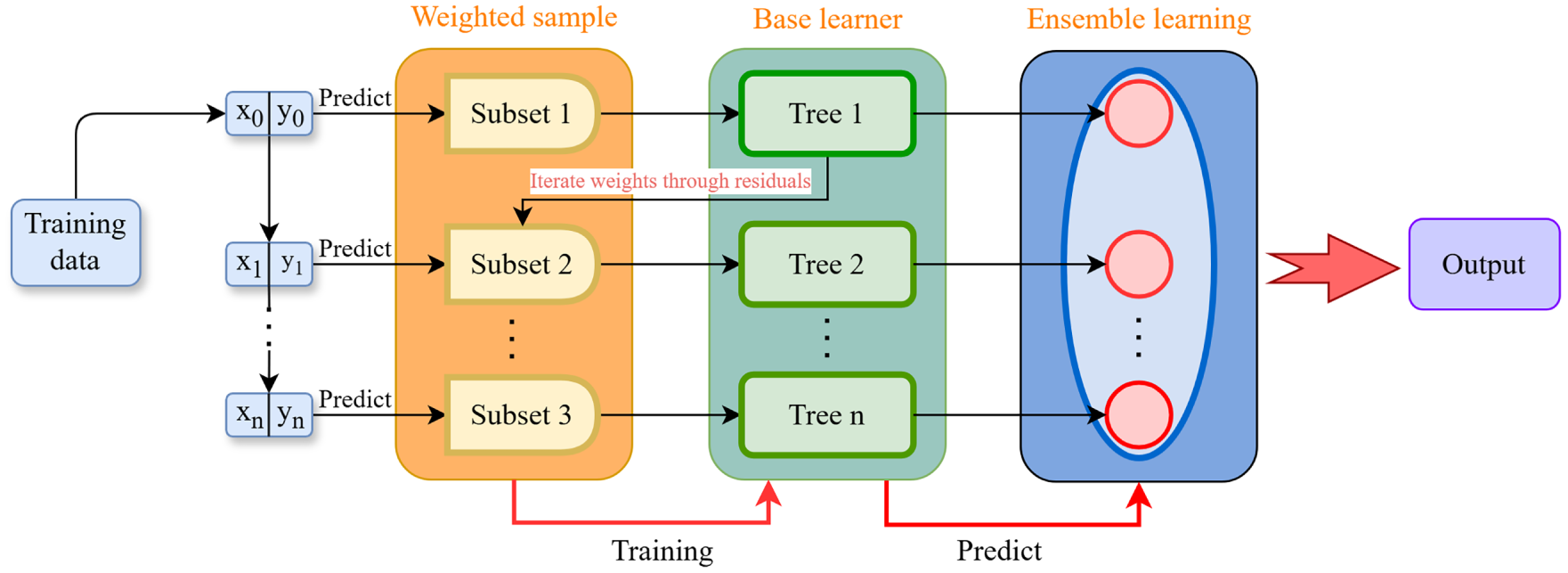
Figure 1: The structure of XGBoost.

XGBoost has demonstrated excellent prediction accuracy and generalization ability in various engineering applications, including rock-property prediction and dam deformation prediction [18,19]. Additionally, impressive scalability is a key feature of XGBoost. It can process data sets of different magnitudes, support different feature types (such as numerical and categorical), and utilize parallel processing to achieve optimal resource utilization to address the needs of diverse tasks [16]. Furthermore, by using regularization strategies, XGBoost can inhibit overfitting of the model [20]. This is particularly significant when dealing with limited sample sizes, as it contributes to better generalization ability of the model and mitigates overfitting to the training data.

At its core, XGBoost seeks to reduce the objective loss function by addressing the optimization task below:

ℒ(ϕ)=∑il(y^i,yi)+∑kΩ(fk)(1)

Ω(f)=γT+12λ‖w‖2(2)

where the function l(y^i, yi) quantifies the loss between the actual value yi and its prediction y^i, and Ω(f) serves as a regularization term to evaluate model complexity and mitigate overfitting. In the Ω(f), γ and λ denote the regularization parameters, T stands for the total number of leaf nodes in the tree, and w is the weight assigned to the leaf. This weight is determined during training and reflects how much that specific leaf contributes to the final prediction result.

2.2 Light Gradient Boosting Machine (LGBM)

Recent studies have demonstrated the applicability of LGBM-based ensemble learning models to dam deformation prediction [21]. As a boosting ensemble model, LGBM integrates multiple weak learners into a more powerful single model. This algorithm was released as open-source by Microsoft in 2017 [22]. Compared to Gradient Boosted Decision Trees (GBDT), LGBM improves computation speed and reduces memory usage while preserving high predictive accuracy [22]. Recent research has further demonstrated the predictive capability and interpretability of LGBM-based models in dam safety analysis [23]. The LGBM model counters the impact of high-dimensional data using an algorithm based on histograms, which also enhances computation speed. Moreover, the training process of LGBM utilizes a parallel voting Decision Tree (DT) method, which enables parallel learning for the model. The structure of LGBM is shown in Fig. 2. For optimization, LGBM utilizes the Leaf-wise strategy to identify appropriate leaves. Regression trees are linked sequentially and can transmit detailed residual information obtained from previous learners in the sequence. The ultimate outcome results come from aggregating these residual trees. The final prediction is created by summing the outputs of the trees modeling residuals. The objective function of LGBM is as follows:

Obj(t)=L(t)+Ω(t)(3)

L(t)=∑i=1n(yit−y^i(t))2(4)

where Ω(t) signifies the regularization term and L(t) stands for the loss function. t denotes the boosting iteration number. The model’s complexity is captured by the regularization term Ω(t). In L(t), yi represents the actual values and y^i signifies the predicted values.

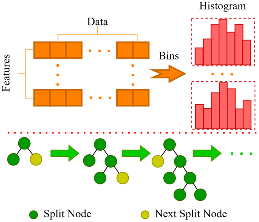
Figure 2: The structure of LGBM.

2.3 Random Forest (RF)

RF is a supervised learning algorithm based on Ensemble Learning, widely used in classification and regression problems. It was proposed by Breiman in 2001 [24]. This method constructs and combines multiple decision trees for prediction, aiming to improve the prediction accuracy and stability of a single decision tree model, and effectively alleviate its problem of overfitting. The structure of RF is shown in Fig. 3. The core mechanism of RF lies in introducing ‘randomness’ to enhance the diversity of the base learners. Specifically, it mainly utilizes two randomization strategies: firstly, to use Bootstrap Aggregating (Bagging) technology to randomly sample the original training dataset with replacement, generating different training subsets for each tree; Secondly, in the process of constructing a decision tree, when each node splits, the optimal segmentation feature is not selected from all features, but from a randomly selected subset of features. Through these two layers of randomness, low correlation between decision trees in the forest is ensured. In the prediction stage, the RF integrates the prediction results of all member trees: for classification tasks, the final category is usually determined by majority voting; for regression tasks, the average of all tree predictions is usually calculated as the final result. This integrated strategy enables RF to have high prediction accuracy, excellent noise tolerance, strong generalization ability, and the ability to evaluate the importance of features.

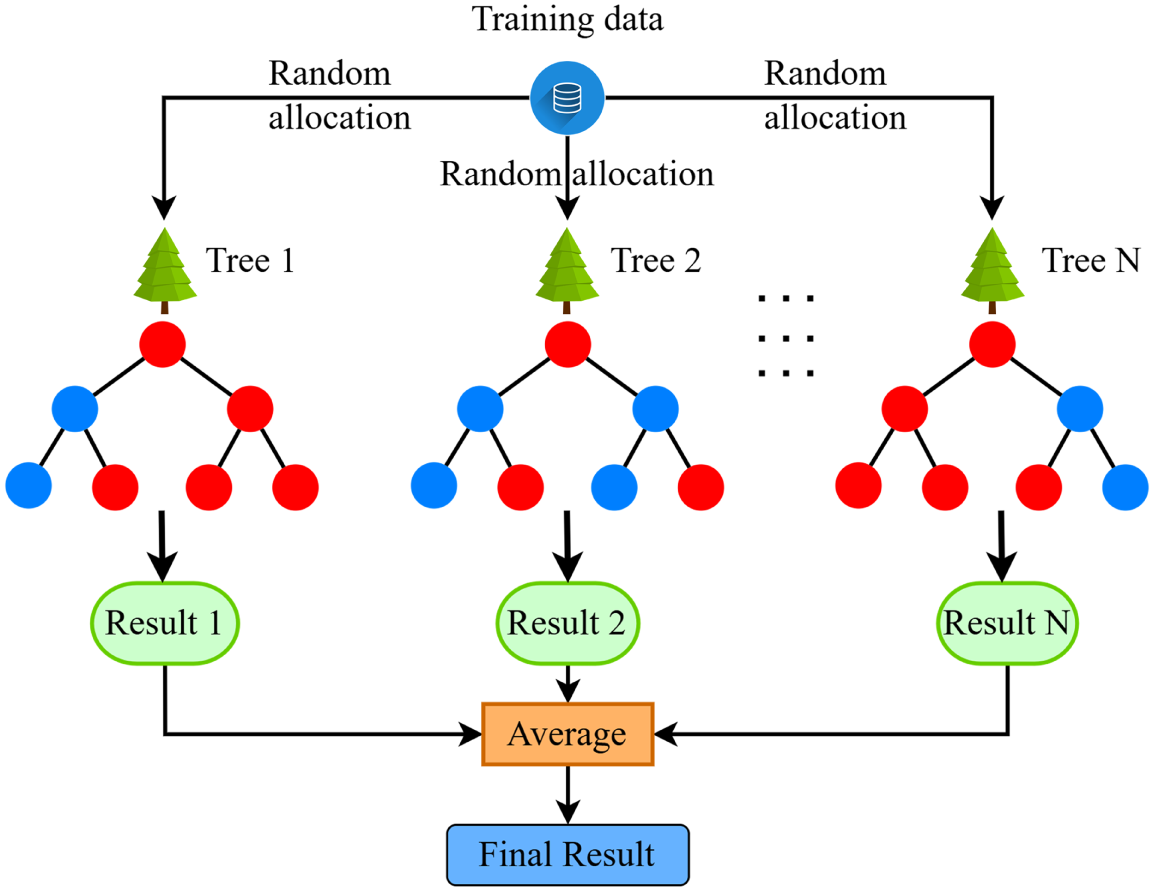
Figure 3: The structure of RF.

2.4 Squirrel Search Algorithm (SSA)

The SSA algorithm was proposed by Jain et al., inspired by the dynamic gliding behavior of flying squirrels during foraging [25]. Flying squirrels utilize their parachute-like skin membrane to regulate aerodynamic forces, effectively controlling lift and drag to achieve complex and economical gliding flight. The algorithm models the inherent behaviors of flying squirrels concerning foraging and food storing, particularly highlighting their gliding actions and specific tree preferences (like acorn tree and hickory) throughout the foraging activity. Furthermore, SSA incorporates a dynamic adaptation strategy for seasonal shifts: In warmer periods, squirrels frequently glide between trees looking for food and saving surplus food. Conversely, winter brings scarcity of food sources and a lack of foliage cover. These conditions lead to less movement of squirrels. Squirrels can only restore their normal activity ability after winter ends. This mechanism reduces the possibility of the algorithm falling into the local optimal solution.

The Squirrel Search Algorithm (SSA) is particularly suitable for this study because dam settlement data is typically highly non-linear and limited in sample size. SSA’s unique “seasonal monitoring condition” dynamically balances global exploration and local exploitation, which effectively prevents the machine learning models from getting trapped in local optima and avoids overfitting during hyperparameter tuning. The algorithm runs as follows:

2.4.1 Individual Location Update Methods

Squirrels adjust their locations through gliding movements between various trees. These squirrels update their positions in three ways. These stages are differentiated based on their gliding start and end positions. The process of squirrels updating their positions is shown in Fig. 4.

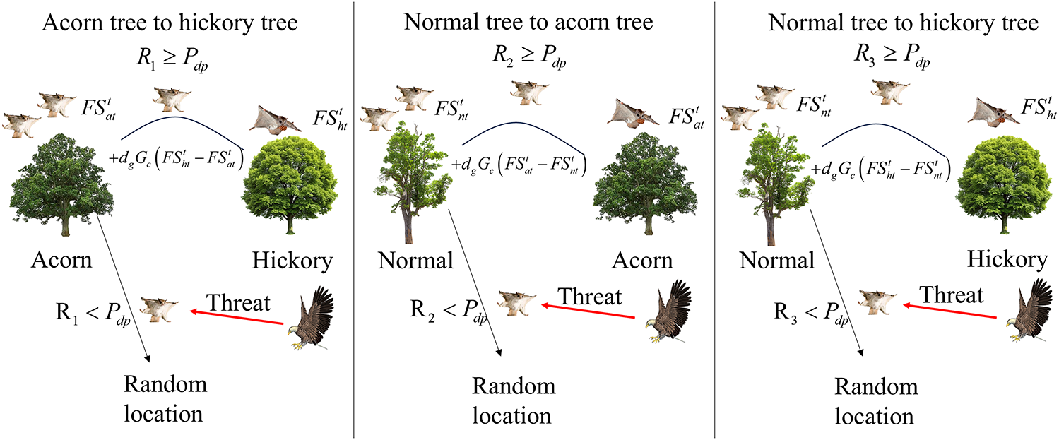
Figure 4: The process of flying squirrels searching for food.

(1) Squirrels on acorn trees move towards the hickory trees in the following way:

FSatt+1={FSatt+dgGc(FShtt−FSatt)R1≥Pdprandom locationotherwise(5)

(2) Squirrels on normal trees move towards the acorn trees in the following way:

FSntt+1={FSntt+dgGc(FSatt−FSntt)R2≥Pdprandom locationotherwise(6)

(3) Squirrels on normal trees move towards hickory trees in the following way

FSntt+1={FSntt+dgGc(FShtt−FSntt)R3≥Pdprandom locationotherwise(7)

where FSat,FSnt, and FSht denote the positions of squirrels on the acorn, normal, and hickory trees, respectively. dg indicates a random gliding distance, Gc refers to a gliding constant, and R1, R2, R3 are randomly generated numbers between 0 and 1. The chance of a predator’s presence is denoted by Pdp.

2.4.2 Season Monitoring Condition

To avoid the algorithm converging to a local optimum, seasonal detection conditions are applied after all individuals update their positions, as detailed below:

Sct=∑k=1d(FSat,kt−FSht,k)2t=1,2,3(8)

Smin=10e−6(365)t/(T/2.5)(9)

where T signifies the total iteration count allowed, and t denotes the present iteration number. If Sct falls below Smin and the seasonal requirement is met, this signals the end of winter. During this phase, any squirrel that has not yet found its food source will randomly move according to the following formula:

FSntnew=FSL+Le´vy(n)×(FSU−FSL)(10)

within the equation, Lévy(n) represents the step size following a Lévy-flight pattern, while FSU and FSL define the maximum and minimum limits for an individual’s location, respectively. The Lévy-flight step size is generated using Mantegna’s algorithm as follows:

Leνy(n)=0.01×α×ra|rb|1β(11)

α=[Γ(1+β)×sin⁡(πβ2)Γ(1+β2)×β×2(β−12)]1β(12)

where ra and rb are two random numbers distributed within the range of [0, 1]. β represents a constant.

3  Data Preparation

3.1 Data Source

The dataset used for model development was compiled from multiple published studies. These studies investigated various aspects of CFRD behavior, including face-slab cracking, long-term deformation, foundation conditions, and parameter back-analysis [26–29]. Further studies focused on three-dimensional dam behavior, statistical characteristics derived from case histories, and dynamic damage of face slabs [30–32]. After data cleaning, records with missing target variable values were removed, yielding a final dataset of 74 cases (Table 1).

Based on previous studies, this study utilizes the following input variables to predict dam crest settlement: dam height (H), intact rockfill strength classification (IRS), foundation condition, valley shape factor (SF), void ratio (e), and measuring period (MP) [33]. Among these, the variables H, SF, e, and MP, as numerical variables, can be directly input into the model, whereas Foundation condition and IRS, as categorical variables, require preprocessing before being input into the model.

The selection of input variables is based on the physical and mechanical mechanisms of rockfill dam deformation. Specifically: (1) Dam height (H) directly determines the self-weight stress within the dam body, which is the primary driving force for settlement; (2) Foundation condition (Fc) governs the stiffness of the supporting base, where softer foundations contribute additional compressive deformation compared to rigid rock foundations; (3) Rockfill strength classification (IRS) reflects the material’s resistance to particle crushing and structural deformation under load; (4) Void ratio (e) indicates the initial volumetric compression potential of the rockfill materials; and (5) Measuring period (MP) captures the time-dependent rheological effects of the dam after construction.

For the processing of categorical features in the dataset, the pandas.get_dummies function from Python’s pandas library was adopted [34]. This function implements one-hot encoding, a technique that converts non-numerical categorical data into a binary (0 or 1). Specifically, for each category in the original feature, this method creates a new column. If a sample belongs to that category, the value in the corresponding new column is 1; otherwise, it is 0. Such an encoding method allows machine learning algorithms to effectively handle non-numeric data. After processing, IRS was converted into three variables: IRS_M-MH, IRS_MH-VH, and IRS_VH, while Foundation condition was transformed into Fc_G and Fc_R. Each sub-variable is composed of 1 and 0, representing presence and absence, respectively.

3.2 Data Augmentation

To enhance the model’s generalization ability and robustness, and to effectively mitigate the overfitting problem on limited training data, a data augmentation strategy based on additive Gaussian noise was designed and implemented. Specifically, for each data point xi (excluding categorical variables) in the original training set, four new synthetic training samples, xij′, were generated by adding noise. This process begins by sampling a noise vector εj of the same dimensionality as xi, from a standard Gaussian distribution with a mean of 0 and a standard deviation of 1. To ensure that the augmented data points remain close to the original ones, this noise is scaled by 5% of the original data point’s value and then added to it. Therefore, the formula for generating an augmented sample is xij′ = xi + (εj · 0.05 · xi). Gaussian noise was chosen because it effectively simulates the random, minor perturbations that arise from various factors in the real world and has been widely validated as an effective regularization technique in machine learning [35–39]. The choice of parameters is crucial: the noise mean μ was set to 0 to ensure the augmentation process does not introduce systematic bias in expectation. This means the average effect of the noise does not shift data points in a specific direction, thus preserving the central tendency of the original data distribution. The standard deviation of the noise applied to each data point was dynamically adjusted to 5% of its own value. This method aims to introduce meaningful, minor changes proportional to the magnitude of the data point, simulating natural fluctuations that may exist in real data. This facilitates effective augmentation while avoiding distortion of the data’s intrinsic structure and information. Four augmented samples were generated for each original data point, expanding the dataset to five times its original size. This number was chosen to provide the model with a sufficiently rich set of training samples, enabling it to explore a broader region of the feature space around the data points. This helps the model learn smoother and more robust decision boundaries while achieving a balance between computational resources and training efficiency. In summary, this data augmentation method is intended to introduce controlled and meaningful variations, compelling the model to learn more essential features and enhancing its predictive accuracy and stability.

3.3 Data Distribution

To verify that data augmentation did not alter the distributional characteristics of the original data, a detailed comparison of the statistical distributions of the datasets before and after augmentation was conducted, as illustrated in Figs. 5 and 6. Morphologically, the frequency histograms of all variables, whether exhibiting a right-skewed distribution like ‘SF’ and ‘MP’ or an approximately normal distribution like ‘e’ and ‘H’, showed no significant visual changes after augmentation. More importantly, from a quantitative standpoint, the measures of central tendency (mean, median) and dispersion (standard deviation) for each variable demonstrated a high degree of stability.

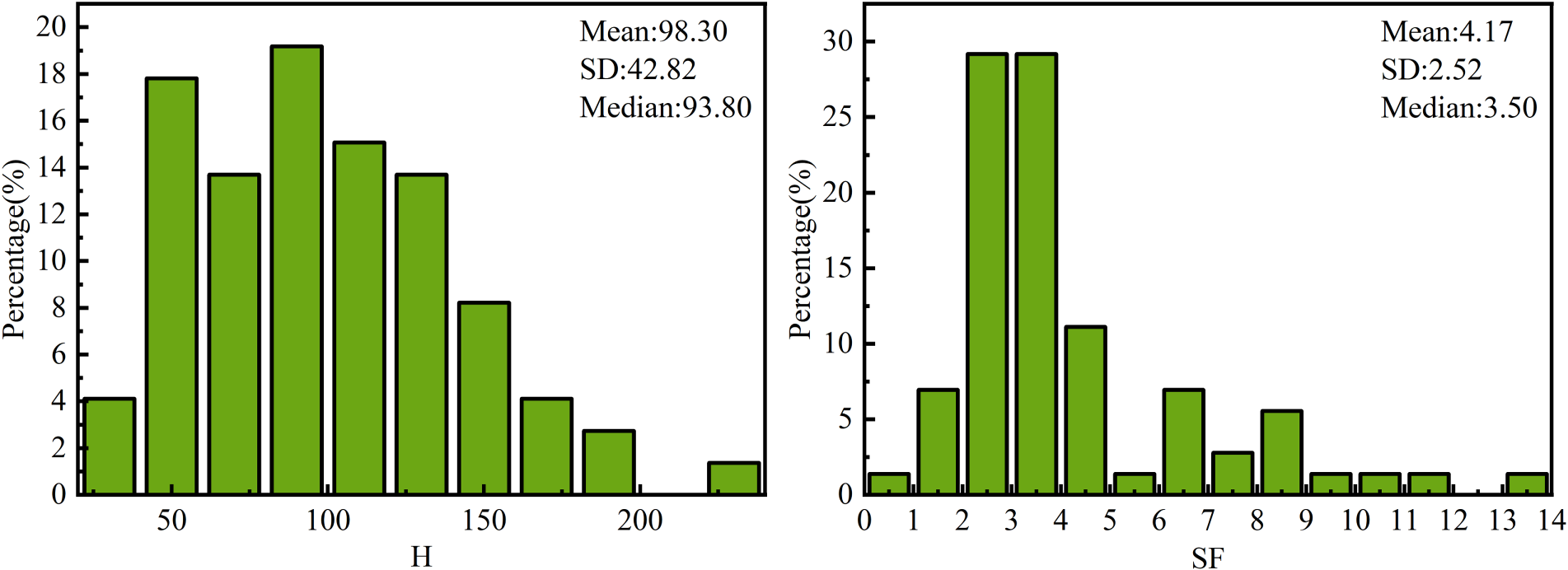
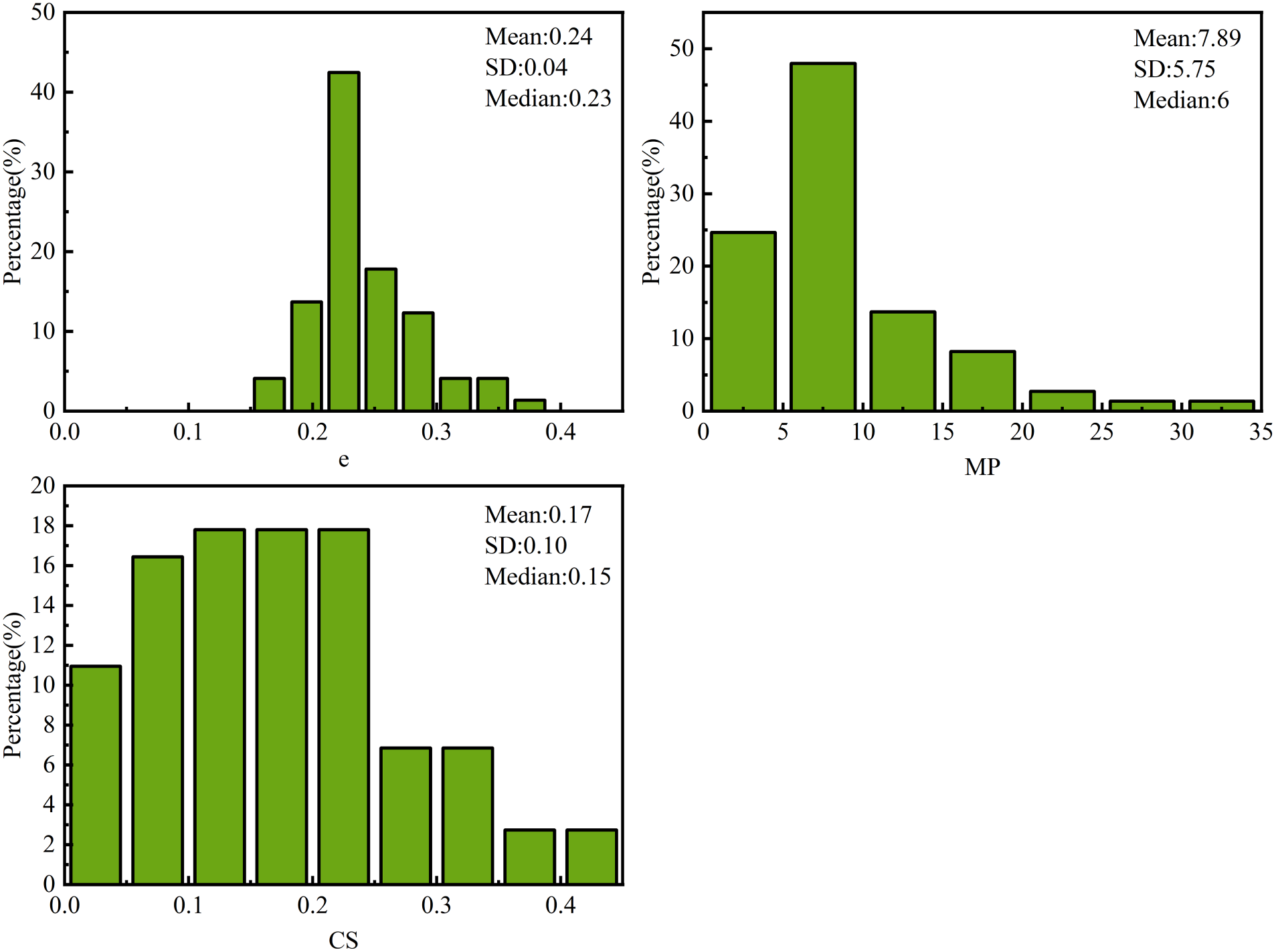
Figure 5: Data distribution before data augmentation.

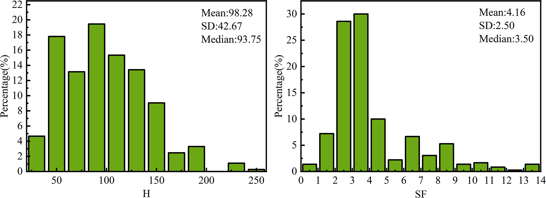
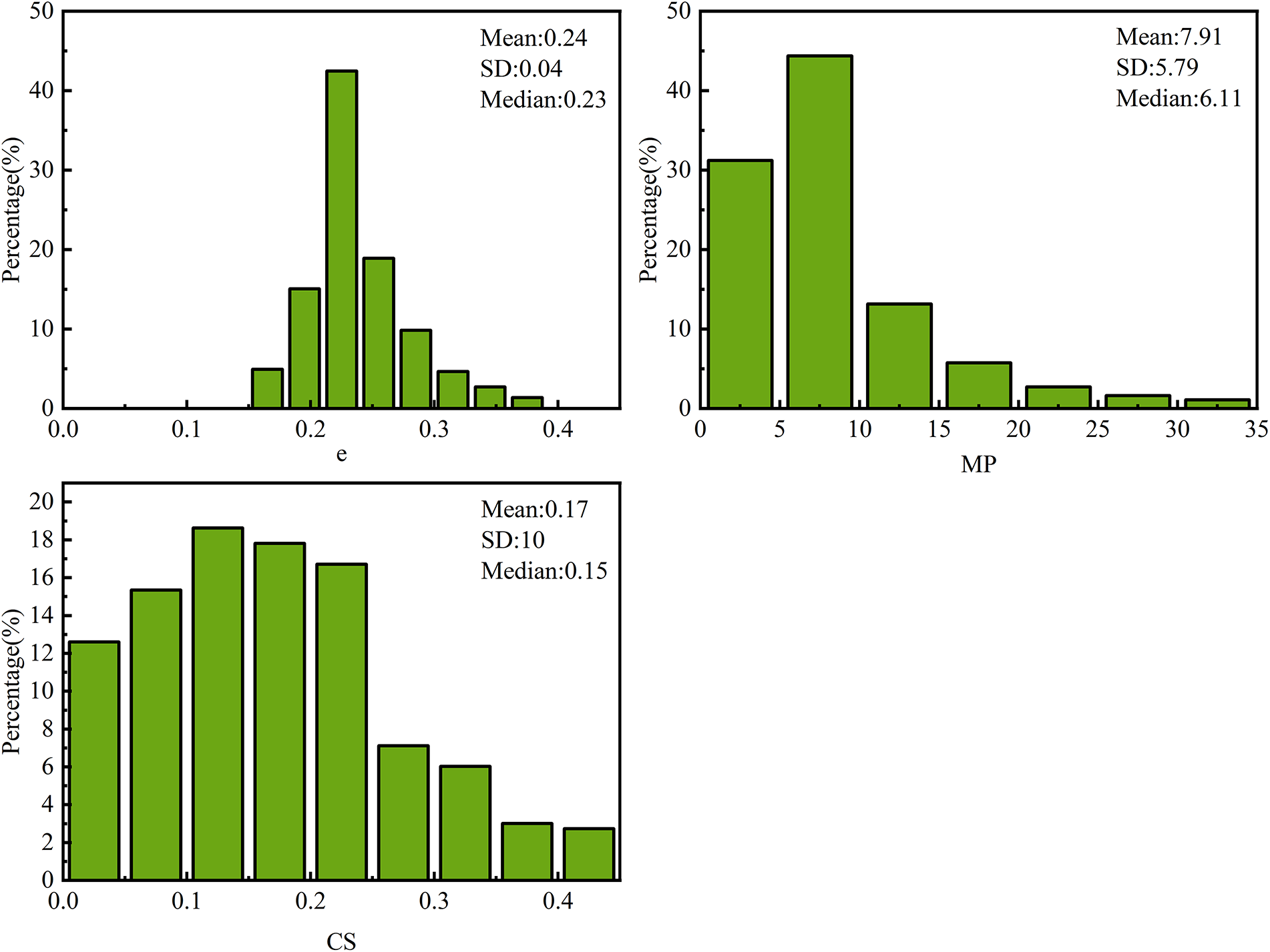
Figure 6: Data distribution after data augmentation.

The observed similarity in these descriptive statistics supports the reasonableness of the adopted data augmentation strategy, suggesting that the augmentation process did not substantially alter the distributional characteristics of the original data while effectively expanding the sample space.

The correlation between variables is depicted in Fig. 7. As can be seen from the figure, significant negative correlations exist among some variables. For instance, strong negative correlations are observed between IRS_VH and IRS_M-MH (−0.78), and between Fc_G and Fc_R (−0.91). Concurrently, some moderate negative correlations (H with SF at −0.46) and positive correlations (e with Fc_R at 0.31, SF with IRS_M-MH at 0.29) were also noted. The correlations between most variable pairs are relatively weak. Although highly negatively correlated variables are present, this is expected because they are subcategories of the same categorical variable, implying a mutually exclusive relationship. Considering the inherent robustness of the selected models to such situations and for the integrity of the feature space, these features are ultimately preserved.

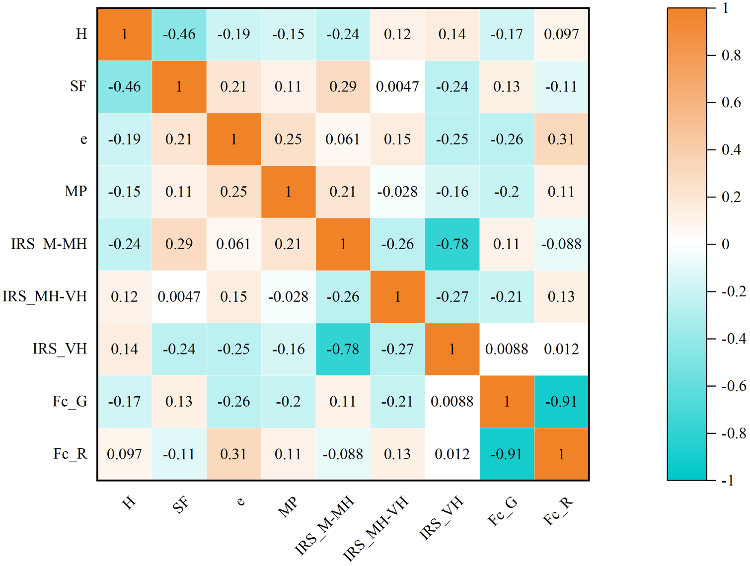
Figure 7: The correlation between input variables.

4  Construction of Models

The tuning of model hyperparameters is important during the training of predictive models. In this study, hyperparameter adjustment was accomplished by optimization with SSA.

4.1 The Hyperparameters Used by Each Model

(1) Hyperparameters used in Xgboost

In XGBoost, n_estimators (number of trees) and learning_rate jointly control the model’s learning iterations and convergence speed, preventing overfitting. max_depth limits the maximum depth of each decision tree, avoiding the learning of noise which can lead to overfitting. reg_lambda penalizes model complexity through L2 regularization, enhancing generalization ability. Meanwhile, subsample controls the proportion of randomly sampled training instances for training each tree. This introduces randomness, training on subsets of data and features reduces the model’s variance and improves its robustness.

(2) Hyperparameters used in LGBM

Within LGBM, n_estimators (the quantity of trees) and learning_rate collectively dictate the model’s learning iterations and convergence rate, serving a similar purpose as in XGBoost. In LightGBM, num_leaves (the number of leaf nodes) acts as the more pivotal parameter for managing tree complexity. This is attributed to LightGBM’s distinct leaf-wise (growing per leaf) strategy, which differs from XGBoost’s level-wise (growing per level) methodology. To counteract overfitting, subsample (the fraction of samples used for fitting individual base learners) is utilized to introduce data randomness, and reg_lambda (L2 regularization) is employed to penalize model complexity.

(3) Hyperparameters used in RF

For RF models, the n_estimators parameter (specifying the number of decision trees in the ensemble) is selected to provide the model with adequate ensemble strength and stability. To manage the complexity of individual trees and mitigate overfitting, max_depth (the maximum depth of each tree), min_samples_split (the minimum number of samples needed to split a node), min_samples_leaf (the minimum number of samples needed at a leaf node) and max_features (the maximum number of features that can be randomly selected when a single tree splits) are tuned; these parameters jointly serve to regularize tree development.

The hyperparameters used in models are shown in Table 2.

4.2 Model Training and Hyperparameter Optimization Process

(1) Data preparation

In the dataset, 80% of the data was allocated to the training set, and 20% was assigned to the test set. To prevent data leakage and ensure an unbiased evaluation of model generalization, the data augmentation was exclusively applied to the training set after the initial train-test split.

(2) Hyperparameters optimization

In this study, the metaheuristic algorithm employed (SSA) is population-based, and the population size is a crucial parameter influencing its optimization process. For each base model to be optimized (RF, LGBM, and XGBoost), the SSA algorithm was independently executed under four different population sizes (25, 50, 75, and 100). This setup aims to investigate the impact of different population sizes on the search efficiency and optimization performance of SSA, in order to identify the optimal hyperparameter combinations for the three models. During the process of optimizing models, the SSA algorithm searches among various combinations of hyperparameters with different population sizes and the performance of each combination was evaluated on the training set using five-fold cross-validation, with the root mean square error (RMSE) serving as the fitness function to be minimized. During this period, the fitness loss value is constantly updated to measure the effectiveness of each combination. As a result, a best set of optimized hyperparameter configurations was determined for each base model under different population sizes, which was then used for subsequent performance comparison and evaluation.

(3) Performance evaluation

To comprehensively evaluate and compare the predictive performance of the different models, this study employed five statistical metrics: the Coefficient of Determination (R2), Root Mean Squared Error (RMSE), Mean Absolute Error (MAE), Variance Accounted For (VAF) and the A-20 index [40–43]. R2 measures the proportion of variance in the actual values explained by the model; a value closer to 1 indicates a better fit of the model. Both RMSE and MAE quantify the average magnitude of prediction errors. RMSE is more sensitive to larger errors, while MAE provides the average absolute magnitude of errors. Smaller values for these two metrics signify higher predictive accuracy of the model. VAF measures the extent to which the model’s predictions can explain the fluctuations in the data. It is typically expressed as a percentage, and a value closer to 100% indicates a better fit. A-20 index represents the proportion of samples for which the predicted values fall within ±20% of the actual values. A higher value for this index indicates a greater prediction accuracy of the model within an acceptable error margin. Collectively, these metrics provide a multi-dimensional and comprehensive assessment of model performance. The mathematical expressions for these metrics are as follows:

R2=1−∑i=1n(yi−y^i)2∑i=1n(yi−y¯i)2(13)

RMSE=1n∑i=1n(yi−y^i)2(14)

MAE=1n∑i=1n|yi−y^i|(15)

VAF=(1−var(yi−y^i)var(yi))×100%(16)

A−20=m20n(17)

where yi signifies the actual value, y^i stands for the predicted value. The mean for all true values is given by yi¯. n represents the total sample size, and m20 indicates the number of instances satisfying 0.8≤y^i/yi≤1.2, where the predicted value falls within ±20% of the actual value.

5  Results and Discussion

5.1 Model Optimization

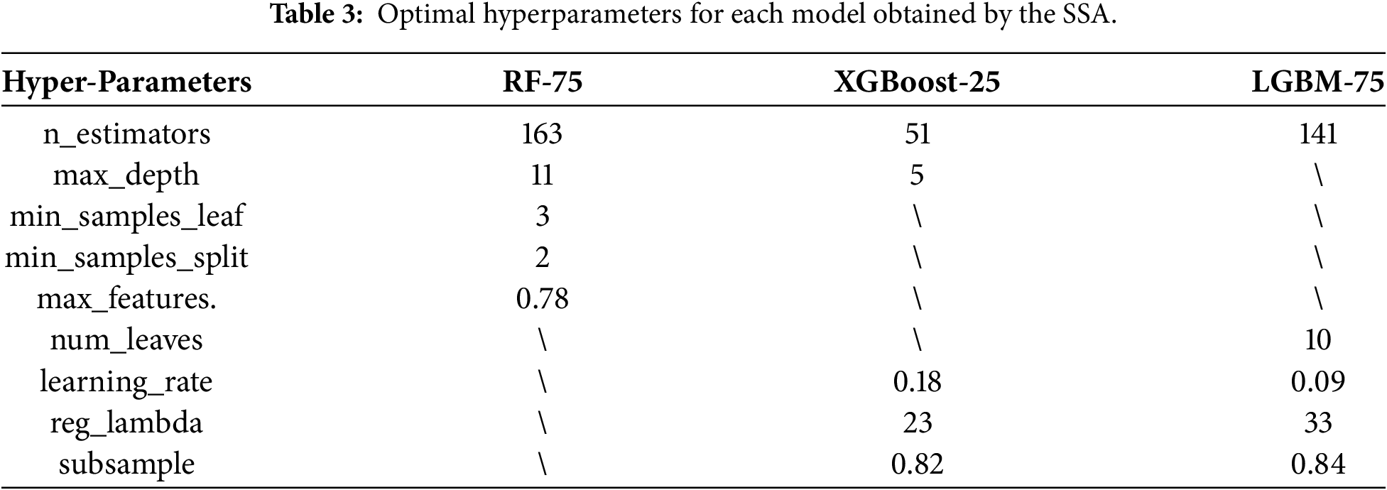
Fig. 8 illustrates the SSA-driven optimization processes for RF, XGBoost, and LGBM. For RF, with a population size of 75, convergence was achieved within 50 iterations, yielding the lowest fitness value. Other population sizes also reached convergence around 50 iterations, exhibiting very similar convergence processes. Their final fitness values are very close but higher than 75 population sizes. For XGBoost, when the population size was 25, convergence was attained around 50 iterations, achieving the lowest fitness value. In contrast, other population sizes also converged around 50 iterations, but their convergence processes were more tortuous, and their final fitness values were higher. For LGBM, with a population size of 75, convergence was reached around 25 iterations, yielding the lowest fitness value. The number of iterations required for convergence varied greatly among different population sizes. For instance, when the population size was 100, convergence was achieved in only 10–15 iterations, whereas with a population size of 50, it took around 40 iterations to converge. Table 3 presents the hyperparameter values for each model that correspond to the lowest fitness value achieved by SSA optimization with different population sizes.

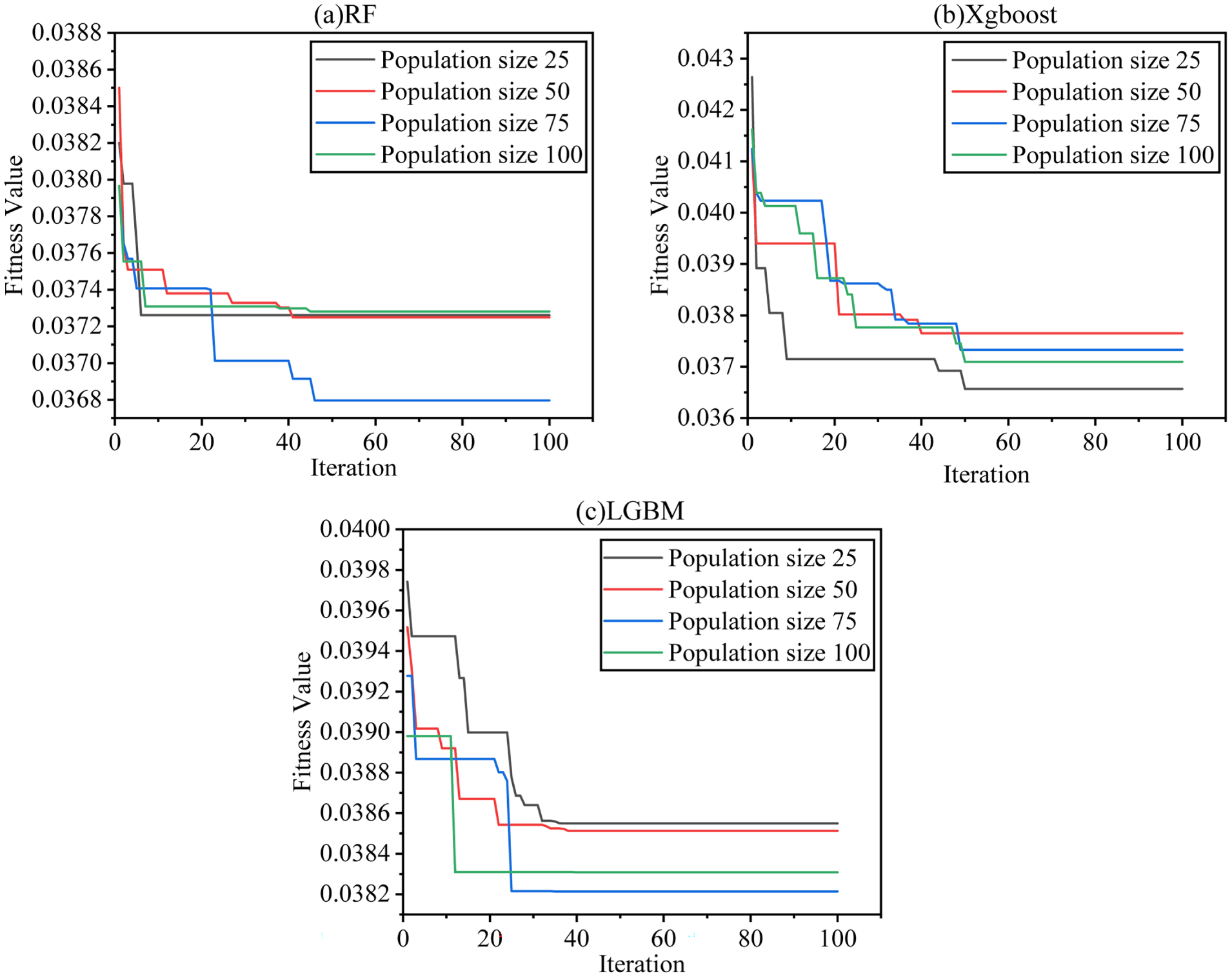
Figure 8: Iterative curves of hybrid models.

5.2 Model Evaluation

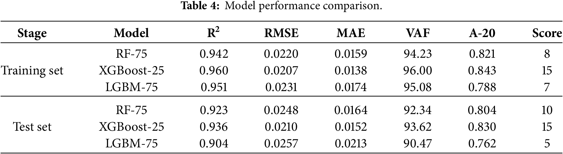
The models that achieved the lowest fitness values under the SSA optimization with different populations in the previous section require further evaluation. For the selection of the optimal model, this study employed the evaluation methodology from Zorlu et al. [44]. This approach involves ranking the models based on each metric and assigning scores accordingly, with the best-performing model achieving the highest rank. Then summarize the scores of all indicators to generate the final total score for each model.

As shown in Table 4, the R2 values on the training sets for the three models are 0.942, 0.960, and 0.951, corresponding to scores of 1, 3, and 2, respectively. This scoring process is repeated for all indicators, and the total score determines the relative performance of each model. For example, RF-75 received a score of 1 for R2, 2 for RMSE, 2 for MAE, 1 for VAF and 2 for A-20 on the training set, and a score of 2 for R2, 2 for RMSE, 2 for MAE, 2 for VAF and 2 for A-20 on the test set, for a total score of 18. Ultimately, XGBoost-25 achieved the highest score (30), followed by RF-75 (18), and finally LGBM-75 (12).

In order to further investigate the differences in performance between models, this study used the nonparametric Friedman test [45,46]. The Friedman test was used to assess the performance differences among the models based on the five evaluation metrics. Fig. 9 presents the average performance ranks of the models across these five evaluation metrics. The performance level decreases from left to right, and a lower average rank indicates better performance.

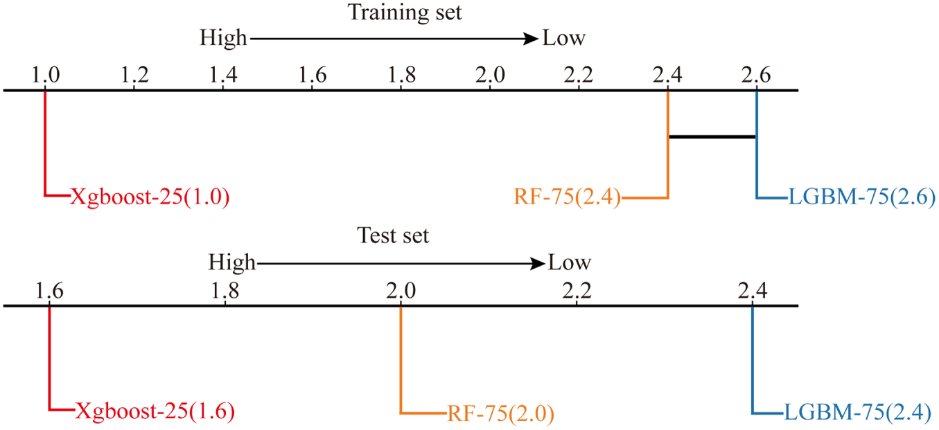
Figure 9: Comparison of different models.

As can be seen from Fig. 9, the XGBoost-25 model performed the best on the training set, ranking first with an average rank of 1.0. The performance of the RF-75 and LGBM-75 models was comparable, and they followed with average ranks of 2.4 and 2.6, respectively. On the test set, the average rank of XGBoost-25 increased, while those of RF-75 and LGBM-75 decreased, but their relative order remained unchanged. The XGBoost-25 model continued to lead with an average rank of 1.6, followed by the RF-75 model with an average rank of 2.0, and the LGBM-75 model with an average rank of 2.4. On the training set, the Friedman test yielded a statistic of 7.600 (p = 0.0224), indicating statistically significant differences among the three models at the 0.05 level. On the test set, the Friedman test yielded a statistic of 1.600 (p = 0.4493), indicating that the performance differences among the three models were not statistically significant. Overall, XGBoost-25 achieved the highest average ranking on both the training and test sets, as shown in Table 4 and Fig. 9.

Fig. 10 visually demonstrates the performance of the three models—XGBoost-25, RF-75, and LGBM-75—on the training and test sets through scatter plots of predicted values and actual values. Each subplot includes a ‘y = x’ diagonal line representing perfect prediction, while two dashed lines (y = 1.2x and y = 0.8x) define the ±20% error bounds. Observing the overall distribution, the predicted points for all three models show a trend of clustering along the diagonal line, indicating their effective predictive capabilities. The vast majority of data points fall within the error band formed by the dashed lines y = 1.2x and y = 0.8x, which indicates a small overall prediction bias. A comparative analysis among the models shows that the XGBoost-25 model (Fig. 10a,b) exhibits the most concentrated data point distribution. For both the training and test sets, its points are most closely clustered about the diagonal, demonstrating the least amount of scatter. This suggests that the predictive results of the XGBoost-25 model are both precise and highly stable, with a consistently high level of accuracy across various samples. By contrast, the RF-75 model (Fig. 10c,d) displays a slightly more dispersed scatter plot, with its data points exhibiting a greater deviation from the diagonal compared to the XGBoost-25 model. The LGBM-75 model (Fig. 10e,f) demonstrates the most scattered distribution. This is particularly evident in the test set, where the data points span a broader range. In summary, a visual analysis of the scatter plot distributions leads to the conclusion that the XGBoost-25 model yields the most precise and reliable predictions. Its compact data point distribution, low dispersion, and strong generalization ability make it the optimal choice among the three models.

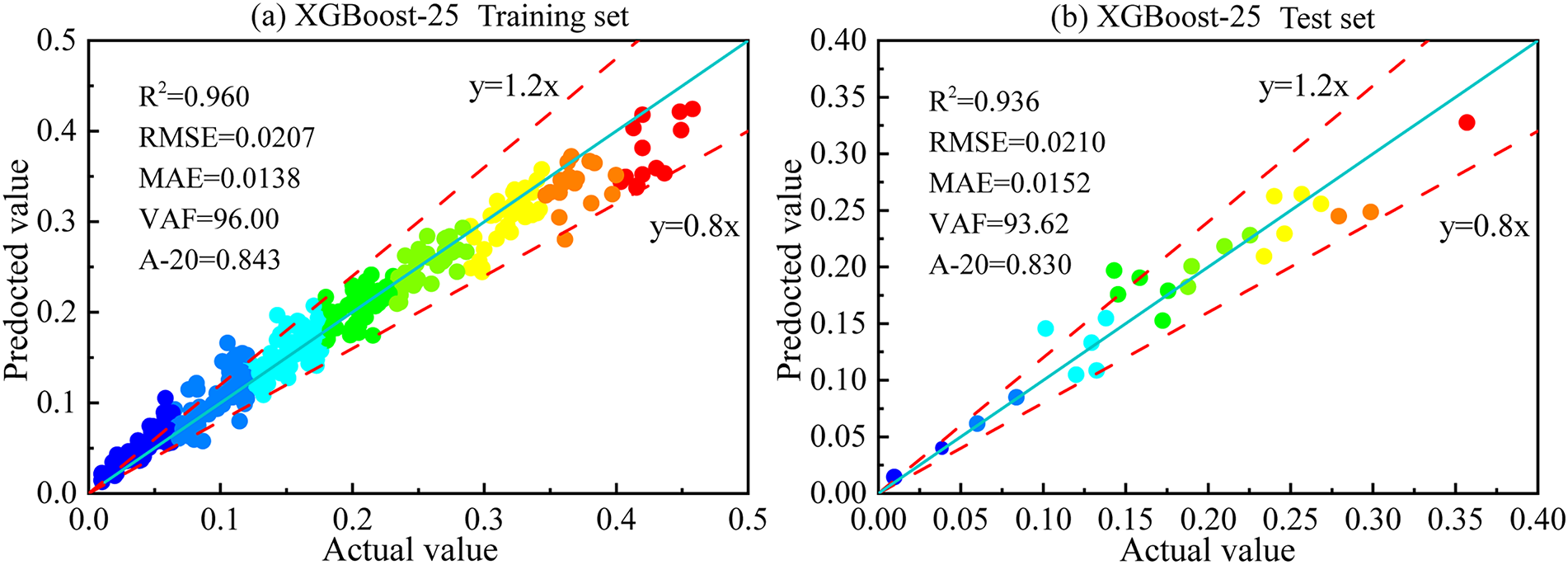
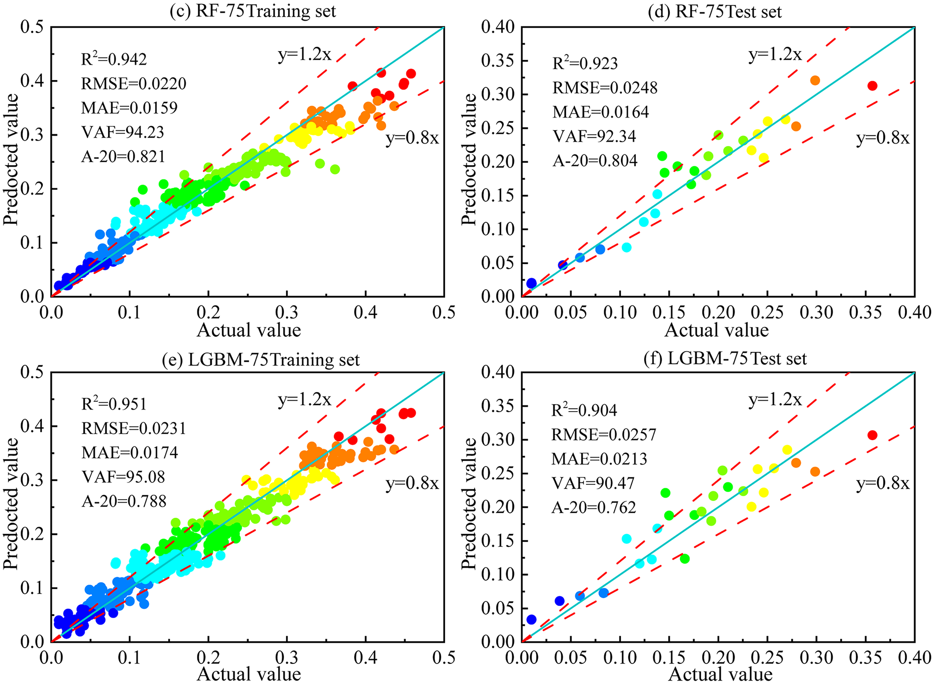
Figure 10: Scatter regression analysis of models on training and test sets.

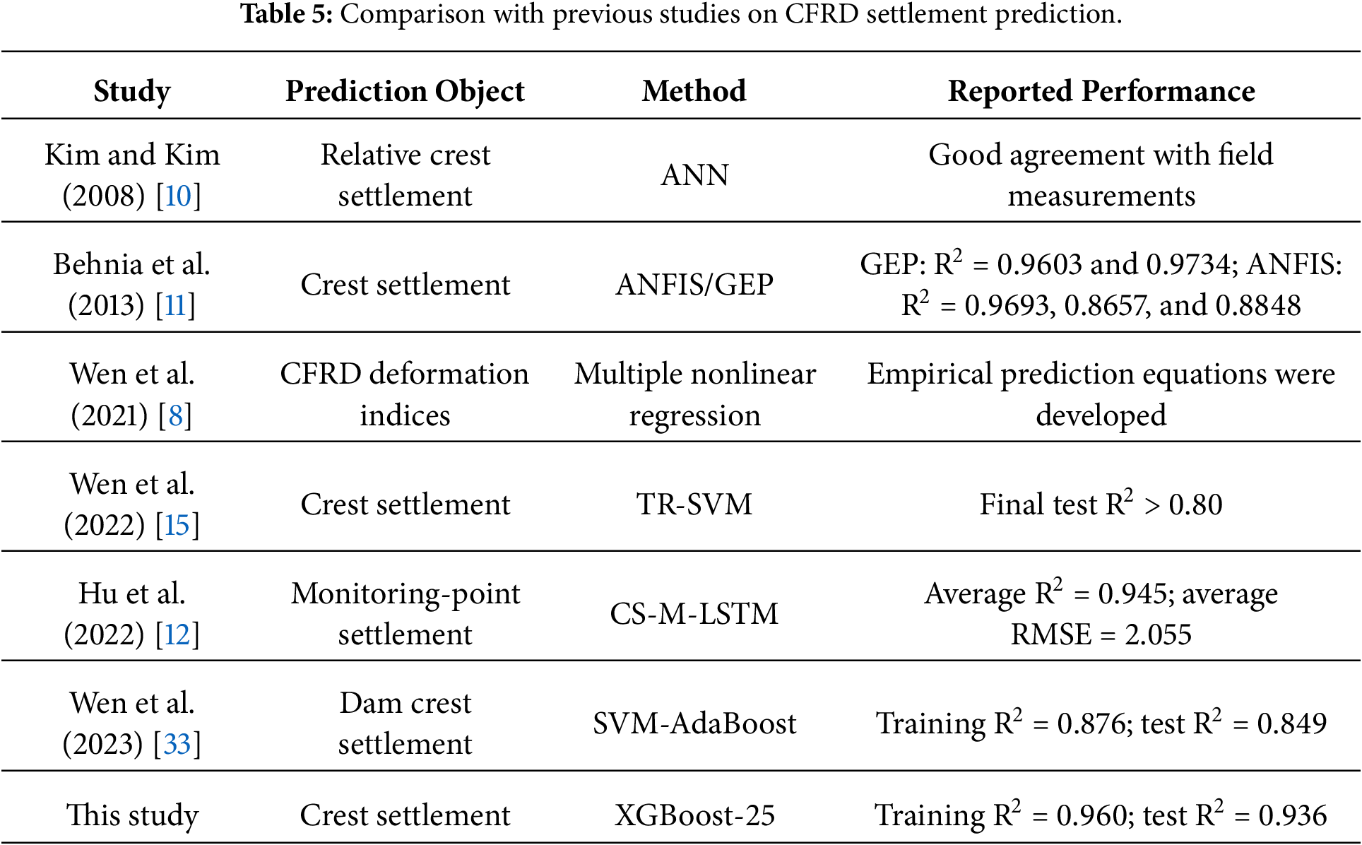
To provide a broader context for the present study, Table 5 summarizes representative empirical and machine-learning-based studies on CFRD settlement prediction. It should be noted that the datasets, target variables, data distributions, and evaluation procedures differ among these studies. Therefore, the reported performance metrics are not directly comparable and are presented only as a descriptive overview of previous research rather than as a statistically rigorous benchmark. Under the dataset partition and evaluation procedure adopted in this study, the proposed XGBoost-25 model achieved a training R2 of 0.960 and a test R2 of 0.936. The corresponding test RMSE, MAE, VAF, and A-20 were 0.0210, 0.0152, 93.62%, and 0.830, respectively. In addition to predictive accuracy, the proposed framework provides model interpretability through SHAP and ICE analyses.

5.3 Model Interpretation

Conducting a contribution analysis on the model helps to understand the degree of contribution of each input variable to the model’s prediction results, thereby enhancing the model’s interpretability [47]. Based on the preceding comparison of model performance, XGBoost-25 was selected as the optimal model for this study. This section will employ several methods, including SHapley Additive exPlanations (SHAP) and the Individual conditional expectation (ICE) plots [48–50], to conduct a contribution analysis of the model, with the aim of revealing its operational mechanism and predictive logic.

Fig. 11 shows the influence of different features on the model’s output. In the plot, each point represents a sample. The vertical axis lists the features, which are ranked by the mean absolute value of their SHAP values, with the most influential feature at the top. The horizontal axis represents the SHAP value, which quantifies the contribution of each sample’s feature value to the prediction. A positive SHAP value indicates that the feature’s value for that sample increases the model’s prediction, while a negative value indicates it decreases the prediction. The color of a point represents the original magnitude of its feature value, with red typically indicating a higher value and blue a lower one. By observing the distribution, color, and corresponding SHAP values of the points, the specific way each feature impacts the model’s prediction can be interpreted.

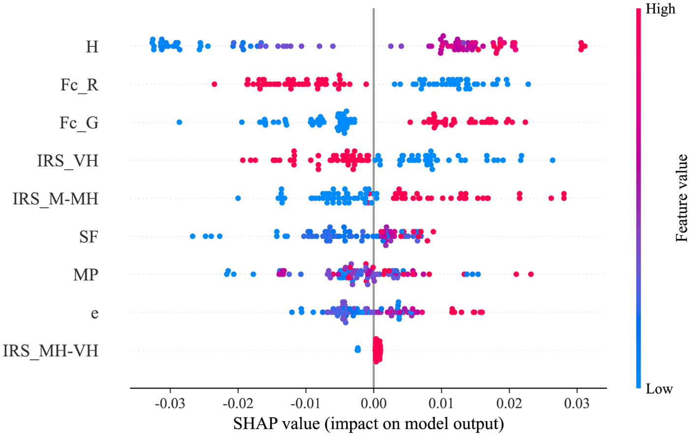
Figure 11: Shapley diagram analysis of XGBoost-25 model.

From the figure, it is evident that H has the greatest impact on the model. Samples with high H values almost all correspond to positive SHAP values, while those with low H values correspond to negative SHAP values, indicating a strong positive correlation between feature H and the model’s prediction. The influence of Fc_R is secondary, but its trend is opposite to that of feature H, showing a clear negative correlation. And its higher feature values are concentrated in the negative SHAP value region. In contrast, Fc_G exhibits a positive correlation, as its higher feature values are concentrated in the positive SHAP value region, which suggests that higher Fc_G values tend to increase the model’s prediction. For IRS_VH, lower feature values tend to have a positive impact, while higher values tend to have a negative impact. IRS_M-MH mainly shows a positive correlation, with its high values concentrated in the positive SHAP value region. The impact of SF is primarily reflected at its lower value. Lower SF values produce significant negative SHAP values, while the impact of high values is not obvious. The influences of MP and e on the model are relatively small, and they exhibit similar trends. Their most data points are clustered around the centerline of SHAP value 0, but they also approximate a trend where larger feature values promote the model’s prediction and smaller values suppress it. Finally, as the least influential feature, the data points for IRS_MH-VH are almost clustered around the centerline, indicating that this feature contributes very little to the model’s prediction.

It should be noted that tree-based ensemble models (e.g., XGBoost) inherently rely on space partitioning and lack mathematical extrapolation capabilities. Consequently, their performance tends to deteriorate in sparse-data regions. An evaluation of the testing set revealed that for a few extreme boundary cases, the prediction errors increased. Therefore, the prediction results should be interpreted with caution when the input parameters of a new project approach or exceed the statistical boundaries of the current training dataset.

Fig. 12 displays the mean absolute SHAP value for each feature. It is clear from the plot that the importance ranking of the features is consistent with that observed in Fig. 11. H has the longest bar, indicating the highest mean absolute SHAP value, undoubtedly becoming the most critical factor affecting the model’s prediction results. Following closely are Fc_R and Fc_G, which also make a significant contribution to the model. The importance of the remaining features, such as IRS_VH, IRS_M-MH, SF, MP, and e, decreases sequentially. The contribution of IRS-MH-VH is the smallest.

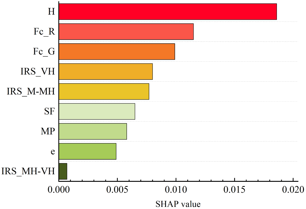
Figure 12: Comparison of the contributions of each input variable.

From the SHAP graph, it can be seen that dam height is the most critical factor affecting settlement, and its SHAP average absolute value far exceeds other variables. The settlement of the dam body is mainly caused by the compression deformation of the rockfill material under self weight stress, and the dam height directly determines the stress level inside the dam body. The higher the dam body, the greater the compressive stress at the bottom and inside, resulting in the compression of internal material pores, which macroscopically manifests as greater settlement. The higher the dam height value in the SHAP diagram, the greater the positive SHAP value, which is a manifestation of this mechanism. Secondly, the foundation conditions (rock foundation, alluvial foundation) also show significant influence. The rock foundation itself has high stiffness and low compressibility, so its SHAP value shows a negative correlation (suppressing settlement). On the contrary, the alluvial foundation is relatively soft, and it will also undergo compression under the load of the dam body, so its SHAP value is positively correlated (promoting settlement). In addition, the changes in SHAP values of the strength (IRS) and porosity ratio (e) of the rockfill material also conform to engineering knowledge: the higher the strength of the rockfill material, the stronger its resistance to deformation and the smaller its settlement; The larger the initial porosity ratio of the material, the greater its potential compression space and the corresponding increase in settlement.

To gain a deeper insight into how the distribution and variation of each feature affect the model’s predictions, Fig. 13 shows the relationship between the model’s predictions and the corresponding changes in input features. For the most important feature H, when its value is below about 100, it stably exerts a suppressive effect on prediction, while as its value increases, it transforms into a significant promoting effect. For Fc_R, when its value changes from 0 to 1, its effect shifts from promoting to suppressive. Conversely, as the value of Fc_G changes from 0 to 1, it exhibits a shift from suppressive to promoting. IRS_VH also shows a similar trend, promoting the prediction when its value is 0 and inhibiting it when its value is 1. For IRS_M-MH, a change in its value from 0 to 1 shifts its effect from suppressive to promoting. For SF, a non-linear relationship is observed, where it only has a significant suppressive effect on the prediction when its value is low, and as its value increases, its impact on the prediction is significantly reduced. For MP, the change in its value did not show a clear or consistent impact on the prediction. For e, when its value is less than about 0.23, it tends to suppress the model’s prediction; when its value is greater than about 0.23, it tends to promote the prediction. Finally, changes in the value of the IRS_MH-VH have the least impact on the prediction results.

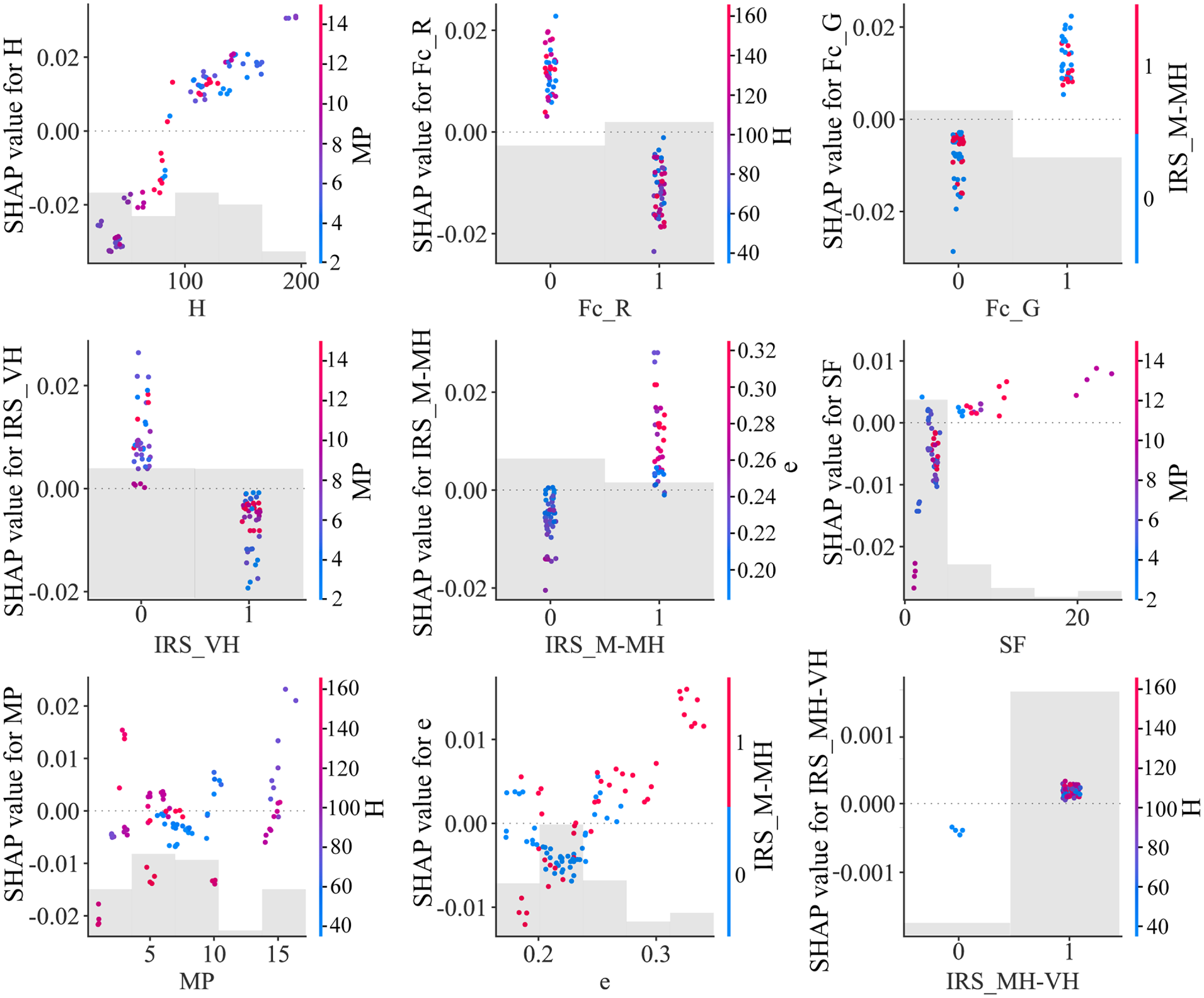
Figure 13: Influence analysis of variables on prediction.

To verify the impact of individual features on model prediction of average performance, Individual Conditional Expectation (ICE) plots were used [49]. As shown in Fig. 14, the results from the plots are highly consistent with the SHAP analysis: Features H, Fc_G, and IRS_M-MH all exhibit a clear positive trend, meaning an increase in their values leads to a rise in the model’s average predicted value. Conversely, Fc_R and IRS_VH show a negative correlation. The non-linear effect of SF was also confirmed, with its influence mainly concentrated in the lower value range. As for MP, e, and IRS_MH-VH, the average influence curve (the red dashed line) is relatively flat, reaffirming their small contribution to the overall model prediction.

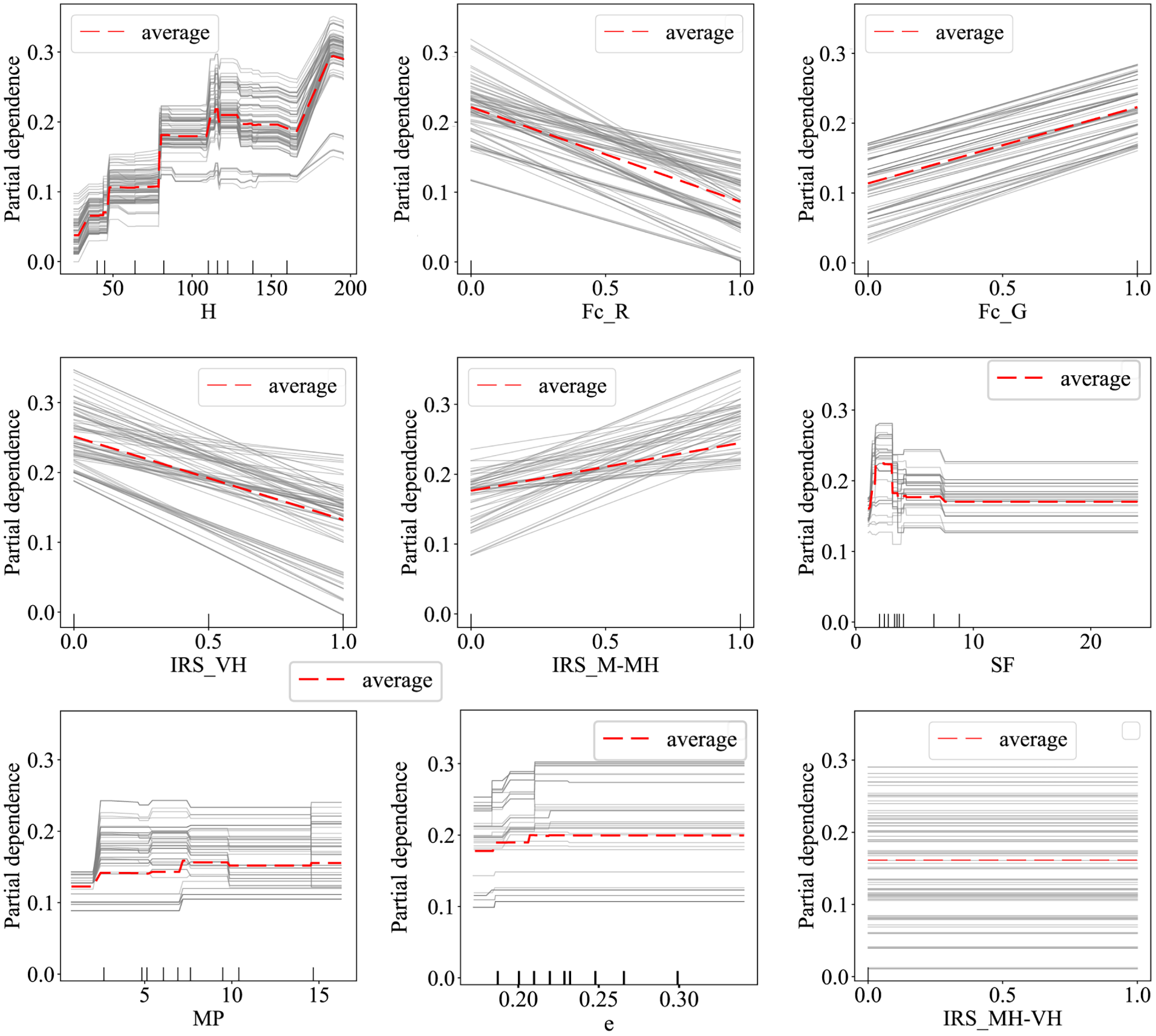
Figure 14: ICE plots for input variables.

6  Conclusions

Given the adverse effects of crest settlement on rockfill dams, it is necessary to develop a settlement prediction model with high accuracy and interpretability. Based on previous studies, this study proposes a new hybrid model (XGBoost-25) with excellent capability in predicting dam crest settlement. The model evaluation results show that XGBoost-25 achieved excellent performance, with an R2 of 0.936, RMSE of 0.0210, MAE of 0.0152, VAF of 93.62%, and an A-20 index of 0.830 on the test set. The contribution analysis indicates that H, Fc_R, Fc_G, IRS_VH, and IRS_M-MH are the most influential variables for predicting dam crest settlement, with H being the most critical variable. In summary, the dam crest settlement prediction model established in this study not only has high prediction accuracy but also excellent interpretability, and can serve as a reference for future researchers.

However, the relatively limited size of the original dataset and the heterogeneity of data collected from different published studies may constrain the generalizability of the proposed model. Future studies should further validate the model using larger and independent datasets from additional CFRDs.

Acknowledgement: None.

Funding Statement:: This research was funded by National Natural Science Foundation of China, grant number 52474121, awarded to Jian Zhou.

Author Contributions:: Xiaoyuan Li: data curation, formal analysis, visualization, and writing—original draft preparation; Ming Xu: data collection, validation, formal analysis, conceptualization, methodology, and software; Shibin Yao: conceptualization and methodology; Su Wang: validation, resources, and writing—review and editing; Jian Zhou: supervision, methodology, project administration, funding acquisition, and writing—review and editing. All authors reviewed and approved the final version of the manuscript.

Availability of Data and Materials: The 74-case crest settlement dataset used in this study is provided in Table 1 and was compiled from previously published studies [26–32]. The trained models, prediction scripts, example input files, and usage instructions are publicly available at: https://github.com/yaoshibin/prediction-of-concrete-faced-rockfill-dams.

Ethics Approval: Not applicable.

Conflicts of Interest:: The authors declare no conflicts of interest.

References

1. Kan ME, Taiebat H. Application of advanced bounding surface plasticity model in static and seismic analyses of Zipingpu Dam. Can Geotech J. 2016;53(3):455–71. doi:10.1139/cgj-2015-0120. [Google Scholar] [CrossRef]

2. Shao C, Gu C, Yang M, Xu Y, Su H. A novel model of dam displacement based on panel data. Struct Control Health Monit. 2018;25(1):e2037. doi:10.1002/stc.2037. [Google Scholar] [CrossRef]

3. Jia JS, Xu Y, Hao JT, Zhang LM. Localizing and quantifying leakage through CFRDs. J Geotech Geoenviron Eng. 2016;142(9):06016007. doi:10.1061/(ASCE)GT.1943-5606.0001501. [Google Scholar] [CrossRef]

4. Kim YS, Seo MW, Lee CW, Kang GC. Deformation characteristics during construction and after impoundment of the CFRD-type Daegok Dam. Korea Eng Geol. 2014;178:1–14. doi:10.1016/j.enggeo.2014.06.009. [Google Scholar] [CrossRef]

5. Liu Y, Zheng D, Cao E, Wu X, Chen Z. Cracking risk analysis of face slabs in concrete face rockfill dams during the operation period. Structures. 2022;40:621–32. doi:10.1016/j.istruc.2022.04.054. [Google Scholar] [CrossRef]

6. Sowers GF. Compressibility of broken rock and the settlement of rockfills. In: Proceedings of the 6th International Conference on Soil Mechanics and Foundation Engineering; 1965 Sep 8–15; Montreal, QC, Canada. p. 561–5. [Google Scholar]

7. Dascal O. Postconstruction deformations of rockfill dams. J Geotech Eng. 1987;113(1):46–59. doi:10.1061/(ASCE)0733-9410(1987)113:1(46). [Google Scholar] [CrossRef]

8. Wen L, Li Y, Chai J. Multiple nonlinear regression models for predicting deformation behavior of concrete-face rockfill dams. Int J Geomech. 2021;21(2):04020253. doi:10.1061/(ASCE)GM.1943-5622.0001912. [Google Scholar] [CrossRef]

9. Zhang Y, Zhong W, Li Y, Wen L, Sun X. ResGRU: a deep learning approach for settlement prediction in CFRD based on the spatiotemporal feature fusion method. Comput Geotech. 2024;173(2):106518. doi:10.1016/j.compgeo.2024.106518. [Google Scholar] [CrossRef]

10. Kim YS, Kim BT. Prediction of relative crest settlement of concrete-faced rockfill dams analyzed using an artificial neural network model. Comput Geotech. 2008;35(3):313–22. doi:10.1016/j.compgeo.2007.09.006. [Google Scholar] [CrossRef]

11. Behnia D, Ahangari K, Noorzad A, Moeinossadat SR. Predicting crest settlement in concrete face rockfill dams using adaptive neuro-fuzzy inference system and gene expression programming intelligent methods. J Zhejiang Univ Sci A. 2013;14(8):589–602. doi:10.1631/jzus.A1200301. [Google Scholar] [CrossRef]

12. Hu Y, Gu C, Meng Z, Shao C, Min Z. Prediction for the settlement of concrete face rockfill dams using optimized LSTM model via correlated monitoring data. Water. 2022;14(14):2157. doi:10.3390/w14142157. [Google Scholar] [CrossRef]

13. Zheng X, Ren T, Lv F, Wang Y, Zheng S. Settlement prediction for concrete face rockfill dams considering major factor mining based on the HHO-VMD-LSTM-SVR model. Water. 2024;16(12):1643. doi:10.3390/w16121643. [Google Scholar] [CrossRef]

14. Su H, Li X, Yang B, Wen Z. Wavelet support vector machine-based prediction model of dam deformation. Mech Syst Signal Process. 2018;110(10):412–27. doi:10.1016/j.ymssp.2018.03.022. [Google Scholar] [CrossRef]

15. Wen L, Li Y, Zhang H, Liu Y, Zhou H. Predicting the crest settlement of concrete face rockfill dams by combining threshold regression and support vector machine. Int J Geomech. 2022;22(6):04022074. doi:10.1061/(ASCE)GM.1943-5622.0002401. [Google Scholar] [CrossRef]

16. Chen T, Guestrin C. XGBoost: a scalable tree boosting system. In: Proceedings of the 22nd ACM SIGKDD International Conference on Knowledge Discovery and Data Mining; 2016 Aug 13–17; San Francisco, CA, USA. p. 785–94. doi:10.1145/2939672.2939785. [Google Scholar] [CrossRef]

17. Shao L, Wang T, Wang Y, Wang Z, Min K. A prediction model and factor importance analysis of multiple measuring points for concrete face rockfill dam during the operation period. Water. 2023;15(6):1081. doi:10.3390/w15061081. [Google Scholar] [CrossRef]

18. Huang S, Yong W, Wang L, Zhou J. From measurement while drilling data to rock strength: a robust LMWOA-XGBoost model for predicting uniaxial compressive strength with SHAP interpretability. Expert Syst Appl. 2026;325:132535. doi:10.1016/j.eswa.2026.132535. [Google Scholar] [CrossRef]

19. Chen X, Hu Y, Wang Y, Zhu X. Dam deformation interval prediction model based on XGBoost. J Hydroelectr Eng. 2024;43(10):121–36. doi:10.11660/slfdxb.20241011. [Google Scholar] [CrossRef]

20. Jing H, He X, Tian Y, Lancia M, Cao G, Crivellari A, et al. Comparison and interpretation of data-driven models for simulating site-specific human-impacted groundwater dynamics in the North China Plain. J Hydrol. 2023;616(8):128751. doi:10.1016/j.jhydrol.2022.128751. [Google Scholar] [CrossRef]

21. Liu M, Wen Z, Su H. Deformation prediction based on denoising techniques and ensemble learning algorithms for concrete dams. Expert Syst Appl. 2024;238:122022. doi:10.1016/j.eswa.2023.122022. [Google Scholar] [CrossRef]

22. Ke G, Meng Q, Finley T, Wang T, Chen W, Ma W, et al. LightGBM: a highly efficient gradient boosting decision tree. In: Proceedings of the 31st International Conference on Neural Information Processing Systems; 2017 Dec 4–9; Long Beach, CA, USA. p. 3149–57. doi:10.5555/3294996.3295074. [Google Scholar] [CrossRef]

23. Li B, Ning J, Yang S, Zhang L. Prediction model for high arch dam stress during the operation period using LightGBM with MSSA and SHAP. Adv Eng Softw. 2024;192:103635. doi:10.1016/j.advengsoft.2024.103635. [Google Scholar] [CrossRef]

24. Breiman L. Random forests. Mach Learn. 2001;45(1):5–32. doi:10.1023/A:1010933404324. [Google Scholar] [CrossRef]

25. Jain M, Singh V, Rani A. A novel nature-inspired algorithm for optimization: squirrel search algorithm. Swarm Evol Comput. 2019;44:148–75. doi:10.1016/j.swevo.2018.02.013. [Google Scholar] [CrossRef]

26. Arici Y. Investigation of the cracking of CFRD face plates. Comput Geotech. 2011;38(7):905–16. doi:10.1016/j.compgeo.2011.06.004. [Google Scholar] [CrossRef]

27. Gan L, Shen ZZ, Xu LQ. Long-term deformation analysis of the Jiudianxia concrete-faced rockfill dam. Arab J Sci Eng. 2014;39(3):1589–98. doi:10.1007/s13369-013-0788-6. [Google Scholar] [CrossRef]

28. Li GY, Miao Z, Mi ZK. A review of foundation condition and design scheme for seepage prevention system of high CFRD built on deep alluvium deposit. Hydro-Sci Eng. 2014;4:1–6. [Google Scholar]

29. Jia Y, Chi S. Back-analysis of soil parameters of the Malutang II concrete face rockfill dam using parallel mutation particle swarm optimization. Comput Geotech. 2015;65:87–96. doi:10.1016/j.compgeo.2014.11.013. [Google Scholar] [CrossRef]

30. Mahabad NM, Imam R, Javanmardi Y, Jalali H. Three-dimensional analysis of a concrete-face rockfill dam. Proc Inst Civ Eng Geotech Eng. 2014;167(4):323–43. doi:10.1680/geng.11.00027. [Google Scholar] [CrossRef]

31. Wen L, Chai J, Xu Z, Qin Y, Li Y. A statistical review of the behaviour of concrete-face rockfill dams based on case histories. Geotechnique. 2018;68(9):749–71. doi:10.1680/jgeot.17.P.095. [Google Scholar] [CrossRef]

32. Xu B, Zou D, Kong X, Hu Z, Zhou Y. Dynamic damage evaluation on the slabs of the concrete faced rockfill dam with the plastic-damage model. Comput Geotech. 2015;65(2):258–65. doi:10.1016/j.compgeo.2015.01.003. [Google Scholar] [CrossRef]

33. Wen L, Li Y, Zhao W, Cao W, Zhang H. Predicting the deformation behaviour of concrete face rockfill dams by combining support vector machine and AdaBoost ensemble algorithm. Comput Geotech. 2023;161(8):105611. doi:10.1016/j.compgeo.2023.105611. [Google Scholar] [CrossRef]

34. McKinney W. Data structures for statistical computing in Python. In: Proceedings of the 9th Python in Science Conference; 2010 Jun 28–Jul 3; Austin, TX, USA. p. 56–61. doi:10.25080/Majora-92bf1922-00a. [Google Scholar] [CrossRef]

35. Bishop CM. Training with noise is equivalent to Tikhonov regularization. Neural Comput. 1995;7(1):108–16. doi:10.1162/neco.1995.7.1.108. [Google Scholar] [CrossRef]

36. Neelakantan A, Vilnis L, Le QV, Sutskever I, Kaiser L, Kurach K, et al. Adding gradient noise improves learning for very deep networks. arXiv:1511.06807. 2015. doi:10.48550/arXiv.1511.06807. [Google Scholar] [CrossRef]

37. Shorten C, Khoshgoftaar TM. A survey on image data augmentation for deep learning. J Big Data. 2019;6(1):60. doi:10.1186/s40537-019-0197-0. [Google Scholar] [CrossRef]

38. Srivastava N, Hinton G, Krizhevsky A, Sutskever I, Salakhutdinov R. Dropout: a simple way to prevent neural networks from overfitting. J Mach Learn Res. 2014;15:1929–58. [Google Scholar]

39. van Dyk DA, Meng XL. The art of data augmentation. J Comput Graph Stat. 2001;10(1):1–50. doi:10.1198/10618600152418584. [Google Scholar] [CrossRef]

40. Nguyen BM, Hoang B, Nguyen T, Nguyen G. nQSV-Net: a novel queuing search variant for global space search and workload modeling. J Ambient Intell Humaniz Comput. 2021;12(1):27–46. doi:10.1007/s12652-020-02849-4. [Google Scholar] [CrossRef]

41. Qiu Y, Zhou J, Khandelwal M, Yang H, Yang P, Li C. Performance evaluation of hybrid WOA-XGBoost, GWO-XGBoost and BO-XGBoost models to predict blast-induced ground vibration. Eng Comput. 2022;38(5):4145–62. doi:10.1007/s00366-021-01393-9. [Google Scholar] [CrossRef]

42. Rezaeineshat A, Monjezi M, Mehrdanesh A, Khandelwal M. Optimization of blasting design in open pit limestone mines with the aim of reducing ground vibration using robust techniques. Geomech Geophys Geo-Energy Geo-Resour. 2020;6(2):40. doi:10.1007/s40948-020-00164-y. [Google Scholar] [CrossRef]

43. Zhou J, Qiu Y, Armaghani DJ, Zhang W, Li C, Zhu S, et al. Predicting TBM penetration rate in hard rock condition: a comparative study among six XGB-based metaheuristic techniques. Geosci Front. 2021;12(3):101091. doi:10.1016/j.gsf.2020.09.020. [Google Scholar] [CrossRef]

44. Zorlu K, Gokceoglu C, Ocakoglu F, Nefeslioglu HA, Acikalin S. Prediction of uniaxial compressive strength of sandstones using petrography-based models. Eng Geol. 2008;96(3):141–58. doi:10.1016/j.enggeo.2007.10.009. [Google Scholar] [CrossRef]

45. Demšar J. Statistical comparisons of classifiers over multiple data sets. J Mach Learn Res. 2006;7:1–30. [Google Scholar]

46. Zhou J, Li X, Mitri HS. Classification of rockburst in underground projects: comparison of ten supervised learning methods. J Comput Civ Eng. 2016;30(5):04016003. doi:10.1061/(ASCE)CP.1943-5487.0000553. [Google Scholar] [CrossRef]

47. Koh PW, Liang P. Understanding black-box predictions via influence functions. In: Proceedings of the 34th International Conference on Machine Learning; 2017 Aug 6–11; Sydney, Australia. p. 1885–94. [Google Scholar]

48. Lundberg SM, Lee SI. A unified approach to interpreting model predictions. Adv Neural Inf Process Syst. 2017;30:4765–74. [Google Scholar]

49. Goldstein A, Kapelner A, Bleich J, Pitkin E. Peeking inside the black box: visualizing statistical learning with plots of individual conditional expectation. J Comput Graph Stat. 2015;24(1):44–65. doi:10.1080/10618600.2014.907095. [Google Scholar] [CrossRef]

50. Winter E. The Shapley value. In: Aumann RJ, Hart S, editors. Handbook of game theory with economic applications. Vol. 3, Amsterdam, The Netherlands: Elsevier; 2002. p. 2025–54. doi:10.1016/S1574-0005(02)03016-3. [Google Scholar] [CrossRef]