
 Login
Login Register
 Submit a Paper
 Propose a Special lssue
 Open Access
ARTICLE
Adaptive Multi-Scale Grid Search with Ensemble Integration for ANN Surrogate Optimization: Application to Multi-Objective Design of Slider–Crank Mechanisms with Springs
1 Faculty of Mechanical Engineering, Industrial University of Ho Chi Minh City, Ho Chi Minh City, Vietnam
2 Faculty of Aerospace Engineering, Le Quy Don Technical University, Hanoi, Vietnam
* Corresponding Author: Van Binh Phung. Email:
(This article belongs to the Special Issue: AI-Enhanced Computational Mechanics and Structural Optimization Methods)
Computer Modeling in Engineering & Sciences 2026, 148(3), 13 https://doi.org/10.32604/cmes.2026.086495
Received 31 May 2026; Accepted 01 September 2026; Issue published 28 September 2026
 View Full Text
 Download PDF
Abstract
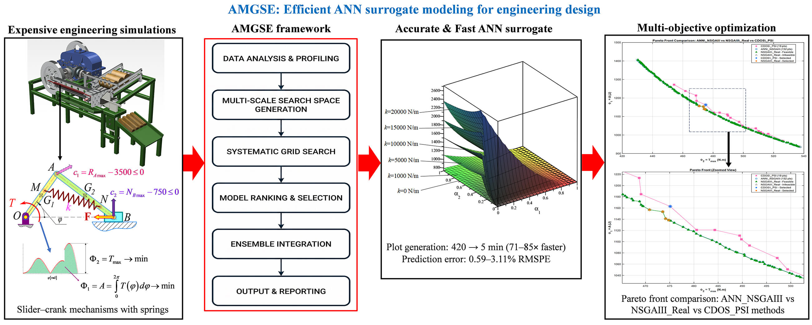
Evaluating objectives and constraints in complex dynamical or multi-physics systems can take minutes to hours per design point, which motivates the use of artificial neural network (ANN) surrogates; in practice, however, their architectures and hyperparameters are still largely chosen by trial and error. This study proposes the Adaptive Multi-scale Grid Search with Ensemble Integration (AMGSE), an automated framework that constructs ANN surrogates from a fixed, previously generated dataset under an explicit training-time budget and without any additional calls to the expensive model. AMGSE couples four explicit decision rules: budget-tiered search scales, dataset-size-triggered complexity scaling, multi-restart training with algorithm-specific restart selection, and a gap-thresholded conditional ensemble rule that withholds ensembling when candidate models are too heterogeneous. Every accepted surrogate must pass an external acceptance test, and every optimization candidate is re-evaluated on the exact model. Under matched search spaces and data partitions over ten independent runs, AMGSE attains mean prediction errors of 0.11%–0.67%, 3.3–10.6 times lower than those of Bayesian optimization, the Tree-structured Parzen Estimator and random search on three of four response functions; Gaussian process regression remains more accurate on three of these smooth, low-dimensional responses, while the AMGSE-selected ANN provides orders-of-magnitude faster batch inference inside the optimization loop. Applied to the multi-objective design of spring-assisted slider-crank mechanisms, the framework enables NSGA-III to return 151 exact-model-verified feasible solutions, of which 150 are mutually non-dominated; these collectively dominate all 19 previously published solutions and improve the hypervolume indicator by 16.1%. Beyond the case study, the same decision protocol was applied without modification to analytic benchmarks with two, six, and eight input dimensions, either certifying a surrogate or declining certification and returning a structured diagnostic. These contrasting outcomes indicate that response multimodality relative to sample density, rather than input dimensionality as such, determined whether the prescribed accuracy could be certified.Graphic Abstract
Keywords
Supplementary Material
Supplementary Material FileIn the design of mechanical systems, machinery, and multi-physics systems, the evaluation of objective functions and constraints often requires computationally expensive numerical simulations such as finite element analysis (FEA), computational fluid dynamics (CFD), or multibody dynamics simulations [1]. In many practical engineering design problems, a single simulation run may take from several hours to several days, depending on the complexity of the model. Consequently, the direct application of multi-objective optimization (MOO) algorithms is extremely challenging [2], as they typically require thousands or even millions of objective function evaluations to find Pareto-optimal solutions.
To address this issue, surrogate modeling (also known as metamodeling) techniques have been developed to replace high-fidelity simulations with computationally efficient approximations. Among these, Artificial Neural Networks (ANNs) are widely used for their strong ability to capture highly nonlinear relationships between design variables and system responses [3–6]. For instance, Han and Kim proposed an ANN-based sequential approximate optimization framework integrated with finite element simulations for metal sheet design, thereby achieving greater efficiency than polynomial response surface methods [7]. In mechanical system design, ANN-based surrogate-assisted multi-objective optimization has also been applied to multibody dynamics problems, where ANN models replace expensive simulations [8]. Similarly, in aerospace engineering, ANN surrogates have been used to substitute CFD simulations in aero-engine nacelle optimization, significantly reducing computational cost during preliminary design [9].
Despite the effectiveness of ANN surrogate models in engineering design optimization, determining an appropriate network architecture remains challenging. In many studies, the ANN structure–including the number of hidden layers, the number of neurons, activation functions, and other hyperparameters–is typically determined through trial-and-error procedures. For example, Massoudi applied ANN surrogate models to describe the relationship between design parameters and compressor performance; however, the ANN architecture was determined by experimentally testing multiple network configurations until satisfactory accuracy was achieved [10]. Similarly, Thaddeus used ANN models to predict the mechanical properties of topology-optimized structures [11], where the network architecture was also selected through repeated testing of different configurations. Another example is the work of Hossein, in which a Taguchi-based approach was used to identify suitable ANN architectures for predicting the elastic properties of short-fiber-reinforced composites [12]. However, this approach still requires evaluating multiple candidate network configurations before selecting the best one. In the context of mechanical system optimization, Lee and Kang also employed ANN surrogate models to optimize vehicle suspension design [13]. Nevertheless, the ANN architecture was still determined through repeated experimentation with various network configurations during training. These examples indicate that trial and error remains a common practice in ANN architecture selection. However, this approach is typically time-consuming and does not guarantee that the selected ANN configuration is optimal for a given engineering problem.
Beyond manual architecture selection, numerous studies in the machine learning community have proposed hyperparameter optimization (HPO) techniques to search for optimal model configurations [14] automatically. A comprehensive overview of hyperparameter optimization techniques is provided in [15]. These approaches can generally be categorized into several groups, including random search-based methods [16], Bayesian optimization, and evolutionary optimization. Traditional approaches, such as grid search and random search, explore predefined hyperparameter spaces but often become inefficient as the number of hyperparameters increases. To overcome this limitation, Bayesian optimization has been proposed as a more efficient strategy for expensive optimization problems by constructing a probabilistic surrogate model–typically a Gaussian process–to approximate the objective function and guide the search for promising hyperparameter configurations through acquisition functions. For example, Snoek et al. demonstrated that Bayesian optimization can significantly reduce the number of evaluations required to optimize the hyperparameters of complex machine learning algorithms [17]. Similarly, Bergstra et al. proposed the Tree-structured Parzen Estimator (TPE), which allows efficient optimization in hierarchical hyperparameter spaces [18]. In addition, evolutionary algorithms and metaheuristic methods, such as genetic algorithms and particle swarm optimization, have been applied to optimize neural network hyperparameters in complex nonlinear engineering problems [19]. Furthermore, López-González et al. proposed a multi-objective evolutionary computation approach that simultaneously optimizes ANN architectures and surrogate model performance in structural engineering applications [20]. Another related approach was presented by Wang et al., who developed an automated framework to optimize neural architectures for physics-informed neural networks [21]. However, in the context of surrogate-based engineering optimization, many existing HPO approaches still require substantial computational resources because they must train multiple ANN models during the search process. This requirement can limit their practical applicability when training data are limited and simulation costs are high.
Another approach to improving the accuracy and robustness of surrogate models is ensemble learning, in which multiple predictive models are combined to form a more reliable, better-generalizing model. Ensemble methods such as bagging, boosting, and stacking have been shown to reduce model variance and improve predictive accuracy in many machine learning applications [22]. In the context of surrogate modeling for engineering design optimization, ensemble surrogate models combine multiple metamodels, such as ANNs, Kriging, and radial basis function (RBF) models, to leverage the strengths of each. For example, Goel et al. proposed an ensemble-of-surrogates framework that integrates multiple metamodels to improve prediction accuracy in surrogate-based design optimization [23]. Similarly, Acar and Rais-Rohani developed an ensemble metamodeling strategy for multi-objective engineering design problems. They demonstrated that combining multiple surrogate models can significantly improve the accuracy of approximations for complex objective functions [24]. However, many existing studies apply ensemble strategies using fixed or simple averaging schemes, which may increase computational cost and may even degrade prediction performance if some component models are significantly less accurate than others. Therefore, developing adaptive ensemble strategies that selectively combine surrogate models based on their predictive quality remains an important research direction for surrogate-based optimization of complex engineering systems.
In recent years, increasing attention has also been devoted to Automated Machine Learning (AutoML), which aims to automate the entire machine learning pipeline, including data preprocessing, model selection, hyperparameter tuning, and ensemble construction [25]. For example, Elsken et al. provided a comprehensive survey of neural architecture search (NAS) methods, where neural network architectures are optimized using strategies such as reinforcement learning, evolutionary algorithms, or gradient-based search [26]. In addition, frameworks such as Auto-WEKA, proposed by Thornton et al. (2013) [27], and Auto-sklearn, proposed by Feurer et al. [28], have been developed to select machine learning models and optimize their hyperparameters automatically. Sun (2025) proposed an automated neural architecture optimization scheme based on probability distribution modeling to optimize ANN architectures and hyperparameters simultaneously [29]. This approach enables efficient exploration of ANN configurations in complex design spaces without manual intervention. Furthermore, Vincent and Jidesh (2023) proposed an evolutionary hyperparameter optimization framework for AutoML systems, in which each individual in the population represents a candidate hyperparameter configuration, and evolutionary operators such as selection, crossover, and mutation are used to search for optimal configurations [30]. A related approach combines Bayesian optimization with evolutionary search strategies. For example, Li et al. (2025) developed a Bayesian Genetic Optimization (BGO) method in which a Bayesian surrogate model approximates the objective function in the hyperparameter space, while genetic operators enhance the search’s exploration capability [31]. Experimental results demonstrated that this approach can outperform traditional strategies such as grid search and random search. However, the method requires training multiple models during the optimization process, leading to relatively high computational cost for simulation-based engineering design problems. Moreover, most existing studies focus primarily on general machine learning applications, whereas the use of such automated approaches in surrogate modeling for mechanical and multiphysics engineering design remains limited. More importantly, many neural architecture search and hyperparameter optimization approaches require substantial computational resources because hundreds or even thousands of network configurations must be trained during the search process. While this cost may be acceptable in large-scale machine learning problems, it becomes a significant limitation in simulation-based engineering design, where training data are typically scarce and expensive to obtain through FEA, CFD, or multibody simulations. Therefore, despite the advances in automated neural architecture design, an effective ANN surrogate modeling framework must simultaneously address several critical challenges: reducing the search cost for ANN configurations in large design spaces, ensuring prediction accuracy and robustness under small-data regimes, and providing explicit mechanisms to manage the trade-off between training cost and surrogate model quality. In this context, developing ANN surrogate modeling methods that can automatically determine suitable network architectures while maintaining computational efficiency and model reliability remains an important research gap in mechanical design optimization.
A review of the existing literature indicates that although ANN surrogate models have been widely applied in engineering design optimization, several critical limitations remain. First, most existing studies focus primarily on maximizing predictive accuracy. In contrast, the trade-off between model accuracy and training cost–a key factor in simulation-based optimization–has not been systematically addressed. Second, many hyperparameter optimization and neural architecture search methods involve large search spaces and high computational costs, which can reduce the practical benefits of surrogate modeling in engineering design problems with limited computational budgets. Third, in many mechanical and multi-physics design problems, training data are typically limited due to the high cost of simulations, making ANN surrogate models prone to overfitting if model complexity is not properly controlled. Consequently, although ANN models are powerful tools for approximating black-box functions in nonlinear mechanical systems, constructing effective and reliable surrogate models remains challenging. The main challenges include:
– Difficulty in selecting appropriate network architectures and hyperparameters in large search spaces.
– Lack of mechanisms to systematically manage the trade-off between training cost and prediction accuracy.
– Risk of overfitting under small-data regimes, which are common in simulation-based engineering design.
– Lack of explicit criteria for determining when ensemble surrogate models should be applied instead of using ensemble strategies by default.
These limitations highlight the need for surrogate modeling frameworks that not only improve ANN prediction accuracy but also effectively manage training cost, model complexity, and training robustness, particularly in data-scarce engineering design scenarios. To address these challenges, this study proposes AMGSE (Adaptive Multi-scale Grid Search with Ensemble Integration)—a comprehensive and automated framework for surrogate-based optimization in computationally expensive engineering problems. The proposed framework introduces four key contributions. First, AMGSE explicitly manages the time budget through a multi-scale grid search strategy. Instead of using a fixed grid search, AMGSE provides four discrete search levels (Micro, Small, Medium, and Large) with increasing numbers of candidate configurations and expected search times ranging from approximately 60 to 600 min. This allows users to select a search level that matches the available computational budget, effectively transforming ANN tuning into a structured and controllable process. Second, AMGSE incorporates adaptive complexity control to mitigate overfitting. When the available dataset is small (Ntotal < 300 samples), the framework automatically scales down the number of neurons using a scaling factor of 0.7 while preserving the overall network structure. This mechanism reduces the risk of over-parameterization and improves model robustness under small-data conditions. Third, AMGSE enhances training robustness through a multi-restart strategy that selects restarts algorithmically. For each candidate configuration, the framework performs multiple independent training runs (R = 8) with different random initializations and, where the training algorithm exposes a validation subset, early stopping is applied. The best restart is then selected by the validation RMSE for trainlm and by the root-mean-square error over the full development set for trainbr, whose toolbox implementation folds the validation partition into the training set, reducing sensitivity to random initialization and enabling fair comparison among configurations. Fourth, AMGSE introduces a conditional ensemble strategy based on gap-thresholding. Instead of applying ensemble learning by default, AMGSE evaluates the performance gap between the top-M candidate models and the best-performing single model. If the maximum gap exceeds 30%, the ensemble strategy is discarded to avoid degrading the best model’s performance. The effectiveness of the AMGSE framework is demonstrated through the multi-objective optimization of dynamic performance, including spring placement and stiffness, in slider–crank mechanisms, a representative case study in mechanical engineering [32].
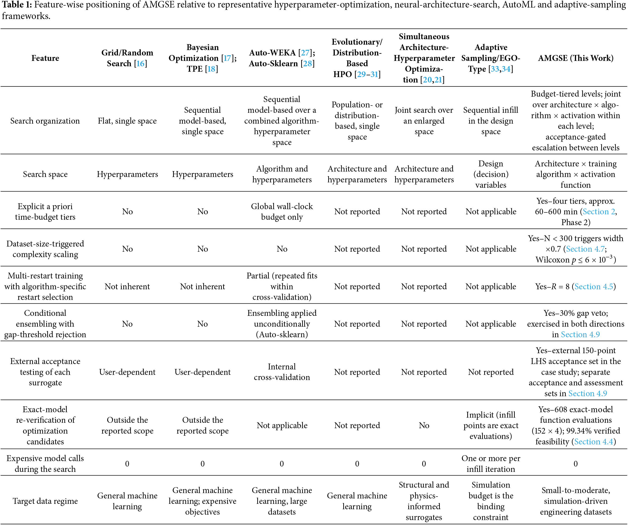
Contribution and scope. We state at the outset what is not claimed. Grid search, multi-restart training, dataset-size-dependent capacity control and inverse-error ensemble weighting are established techniques, and no novelty is claimed for any of them individually. The contribution of this work is stated as four items, each tied to specific evidence. (C1) A decision protocol rather than a heuristic recipe: four tightly specified, auditable rules–budget-tiered search scales, a dataset-size-triggered capacity rule, restart-and-select, and a gap-thresholded ensemble veto–together with the complete pseudo-code of Appendix C, make the surrogate-construction pipeline reproducible without case-by-case intervention once the search scales, thresholds and acceptance tolerance have been specified. Table 1 positions this conjunction feature-by-feature against representative hyperparameter optimization, neural architecture search, AutoML, and adaptive sampling frameworks. (C2) A cost- and variance-justified hierarchy, empirically examined in two complementary settings: a fivefold larger simultaneous search on the case study (Section 4.6.2), and the escalation rule itself exercised on analytic benchmarks (Section 4.9). (C3) A two-stage verification protocol in which every surrogate accepted for downstream use must pass an external acceptance test before optimization, failing which the framework returns a structured diagnostic, an untouched assessment set being recommended whenever escalation occurs and implemented in the benchmark study of Section 4.9, and every optimization candidate is re-evaluated on the exact model afterwards; machine-learning studies generally stop at held-out test error, whereas in mechanism design a constraint violation means an unusable device. (C4) A verifiable advance on published results for this problem class: the exact-model-verified non-dominated front dominates all 19 CDOS-PSI solutions of [32] with no reverse dominance and improves the hypervolume indicator by 16.1% (Section 4.4). We further note that this manuscript reports findings unfavorable to its own framework—the ablation study of Section 4.5, the surrogate-level comparison of Section 4.3.3, and the sampling analysis of Section 4.7—because delineating where a framework does and does not work is, in our view, part of what a methodological contribution owes its readers.
Scope of the framework. AMGSE operates on a fixed, previously generated dataset and never invokes the expensive high-fidelity model during hyperparameter search; the exact model is used offline only to generate the development and independent assessment data and to verify the final Pareto candidates. The framework, therefore, does not aim to reduce the number of expensive simulations—a goal pursued by surrogate-assisted optimization with adaptive sampling and by multi-objective hyperparameter optimization approaches that jointly address accuracy, overfitting, and evaluation cost [14]–but to extract the most reliable surrogate from a given dataset under an explicit training-time budget. The two goals are complementary rather than competing. We emphasize, because it is central to how the present results should be read, that the search performed by AMGSE takes place entirely in the ANN configuration space and consumes zero evaluations of the expensive model (Section 4.6); optimizer-driven selection of new design points, which addresses the complementary problem of data acquisition, is analyzed separately in Section 4.7.
Relation to our previous work. Reference [32] contributed the mathematical model of the spring-assisted slider–crank mechanism, the 2048-point dataset, and the 19 CDOS-PSI Pareto solutions, which are reused here solely as training data and as a comparison baseline. All methodological content of the present study–the AMGSE framework, the surrogate-construction protocol, the verification methodology, and the NSGA-III-based optimization results–is new and does not overlap with [32].
Table 1 makes this positioning explicit rather than declarative. Entries for prior work reflect features documented in the cited publications; “Not reported” indicates that a feature is not documented in the cited source, and each entry has been checked against the original publication (the full, unabridged version of this comparison is retained in Supplementary Section S9).
We state plainly that grid search, multi-restart training, capacity control, and ensembling are all established techniques; the differentiator is the combination of rows 3–9 into a single deterministic, auditable decision protocol. Partial overlaps exist and are acknowledged: Auto-sklearn does construct ensembles, but unconditionally and without a quality-gap rejection rule; Bayesian optimization is designed for expensive objectives but provides no dataset-size-dependent capacity control; ensemble-of-surrogates methods [23,24] combine metamodels but perform no architecture search; and [20,21] optimize architectures and hyperparameters simultaneously over a joint space, but without per-function acceptance certification, a priori budget tiers, or exact-model re-verification of the optimization outcome. To the best of our knowledge, none of the frameworks compared here addresses the small-data, simulation-driven engineering regime under a single explicit and reproducible decision protocol.
From a broader perspective, AMGSE not only improves surrogate model accuracy and reduces computational cost but also enables the effective application of advanced multi-objective evolutionary algorithms (MOEA) in black-box optimization problems with extremely expensive simulations. In this way, the proposed framework helps bridge the gap between advanced optimization theory and practical engineering applications, where high simulation costs remain a major barrier to adopting sophisticated optimization techniques.
2 Methodology: Proposed AMGSE Framework
Terminological clarification. The “grid” in AMGSE is a grid over the ANN configuration space (architectures × training algorithms × activation functions); traversing it requires no evaluation of the expensive model. It is not a grid over the design-variable space: the design-space samples are exogenous to AMGSE–here, the 2048-point dataset inherited from [32]–and AMGSE adds zero exact-model calls during its search. Throughout this study, the term configuration-space grid search is used whenever the distinction matters.
2.1 Overview of the Six-Phase Framework
This section introduces the Adaptive Multi-scale Grid Search with Ensemble Integration (AMGSE) framework, a systematic methodology designed to optimize artificial neural network (ANN) configurations for surrogate modeling applications (Fig. 1). The framework addresses three fundamental challenges in contemporary ANN optimization: the time–quality trade-off inherent in hyperparameter search, the need for adaptive model complexity calibration based on dataset characteristics, and the characterization of inter-model prediction disagreement in practical deployment environments. Unlike traditional grid search methods that operate on fixed configuration spaces without explicit management of computational budgets, AMGSE employs a hierarchical multi-scale strategy that enables practitioners to balance search thoroughness against available computational resources explicitly. Compared with conventional ANN hyperparameter tuning approaches, AMGSE organizes three mechanisms under explicit decision rules: time-budget management, adaptive complexity control for small datasets, and conditional ensemble integration. None of these mechanisms is new in itself; the claimed contribution is their integration under a single auditable protocol, as set out in Section 1 and shown in Table 1.
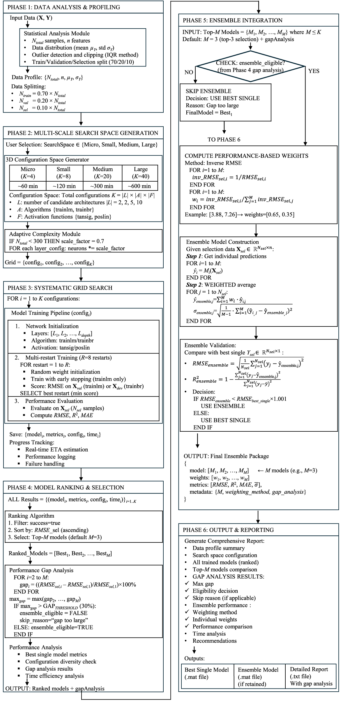
Figure 1: Flowchart of adaptive multi-scale grid search with ensemble integration (AMGSE) framework.
The framework operates through six interconnected phases that progressively transform raw input data into validated predictive models with an ensemble-based disagreement indicator. Beginning with comprehensive data profiling, the methodology constructs a structured three-dimensional configuration space spanning layer architectures, training algorithms, and activation functions. An adaptive complexity module automatically adjusts network capacity based on dataset size to mitigate the risk of overfitting in data-scarce regimes. Systematic grid search with multi-restart training explores this configuration space, followed by performance-based ranking and ensemble integration. The ensemble mechanism not only combines multiple high-quality models to improve predictive accuracy but also provides sample-wise inter-model disagreement indicators via prediction variance analysis, enabling risk-aware decision-making in practical engineering applications.
The framework organizes explicit time–quality trade-off management through four discrete search scales (Micro, Small, Medium, Large), adaptive complexity adjustment informed by statistical learning principles, and built-in ensemble construction with ensemble-disagreement characterization. The following subsections describe each phase of the methodology in detail and establish the conceptual workflow illustrated in Fig. 1, which summarizes the progression from initial data profiling to final surrogate model deployment.
Phase 1 (Data Profiling) establishes a data foundation through comprehensive statistical characterization, including outlier detection via the interquartile range (IQR) method, and randomized partitioning into training (70%), validation (20%), and selection (10%) subsets. This rigorous separation prevents information leakage between model development and final performance evaluation.
Phase 2 (Multi-Scale Search Space Generation) introduces the framework’s primary design feature: explicit time-quality trade-off management through four discrete search scales (Micro: ~60 min, Small: ~120 min, Medium: ~300 min, Large: ~600 min), each exploring K = {4, 8, 20, 40} configurations respectively across three hyperparameter dimensions: network architectures (layer sizes and depths), training algorithms (Levenberg-Marquardt and Bayesian regularization), and activation functions (hyperbolic tangent and positive linear; the Micro scale explores the hyperbolic tangent only, giving K = 4, while both activations are explored from the Small scale upward). An adaptive complexity module automatically reduces network capacity when the total dataset size falls below 300 samples (scaling factor 0.7), mitigating overfitting in data-scarce regimes while preserving representational capability.
Phase 3 (Systematic Grid Search) executes rigorous training for each configuration using multi-restart initialization (R = 8 independent training runs with different random seeds) to overcome the sensitivity of neural networks to initial weights. For each configuration, the best restart is selected by the validation RMSE for trainlm and by the development-set RMSE for trainbr, then evaluated on the isolated selection split using three complementary metrics: root mean squared error (RMSE), coefficient of determination (R2), and mean absolute error (MAE).
Phase 4 (Model Ranking and Gap Analysis) ranks all successfully trained configurations by selection-split RMSE and performs critical gap analysis to determine ensemble eligibility. An explicit decision criterion evaluates whether the top-M candidate models (typically M = 3) exhibit sufficient quality homogeneity by comparing their performance against a 30% gap threshold. If the maximum performance gap among top models exceeds this threshold, ensemble construction is skipped to prevent degradation of the best single model; otherwise, proceeding with ensemble integration reduces variance through complementary predictions.
Phase 5 (Ensemble Integration and Ensemble-Disagreement Characterization) constructs weighted ensembles using inverse-RMSE weighting when eligible, combining M constituent models into a single predictor with explicit per-sample disagreement characterization through prediction variance analysis. This supports risk-aware decision-making through an input-specific inter-model disagreement indicator that distinguishes regions of strong model agreement from regions of high disagreement, where model predictions diverge substantially.
Phase 6 (Comprehensive Output) generates complete documentation, including ranked model listings, gap analysis results, ensemble performance comparison, and deployment recommendations, along with trained model files (*.mat format) ready for immediate application in downstream multi-objective optimization.
The complete procedural details and mathematical formulations for all six phases are provided in the Supplementary Material (Sections S1–S6); the governing equations are summarized in Appendix B. The symbols and mathematical notation used throughout the paper are summarized in Table A1 of Appendix B.
2.2 Rationale for Hierarchical Escalation over Simultaneous Joint Search
Simultaneous optimization of architectures and hyperparameters over a single enlarged space, as pursued in [20,29], and the escalation strategy adopted here answer different decision questions. The former seeks the most accurate configuration that is affordable within a global budget; the latter seeks the least expensive search level that meets a prescribed per-function accuracy tolerance ε. When several objective and constraint functions of differing difficulty must each be certified–four functions in the present case study–a per-function decision is the natural formulation. We first remove a possible ambiguity: within each level, architectures, training algorithms, and activation functions are optimized simultaneously over the full Cartesian product; the hierarchy concerns complexity scales separated by an acceptance test, not sequential, one-hyperparameter-at-a-time optimization. Selecting the largest tier at the outset, with escalation disabled, recovers the simultaneous full-space search as a special case. Hence, the hierarchy is a resource-allocation protocol and does not restrict the class of searchable hypotheses.
The rationale rests on three arguments. Statistically, complexity-ordered search is motivated by the principle of structural risk minimization: ranking a large number of candidates against a single finite internal validation split inflates selection-induced optimism. This is not a hypothetical concern here—Section 4.3.2 documents it on RA,max, and the ablation study of Section 4.5 shows that on Φ2 a single-restart variant attained 0.091% against 0.224% for the full framework. A flat search over a larger configuration space precisely amplifies this effect, whereas escalation limits the number of ranked candidates unless the acceptance test demands more. Economically, the expected escalation cost is
3 Application of the AMGSE Framework
3.1 ANN-Based Mathematical Optimization Model Construction Using AMGSE Framework with Hierarchical Multi-Scale Refinement
This flowchart illustrates a systematic framework for constructing mathematical optimization models in which all objective functions {Φ1, Φ2, …, ΦN}, inequality constraint functions {c1, c2, …, cP} ≤ 0, and equality constraint functions {ceq1, ceq2, …, ceqQ} = 0 are approximated using Artificial Neural Network (ANN) surrogate models (Fig. 2). The framework employs the AMGSE (Adaptive Multi-scale Grid Search with Ensemble Integration) methodology as a self-contained modeling engine, ensuring that each surrogate function meets predefined accuracy requirements before being incorporated into the final optimization formulation. This approach is particularly suitable for problems where explicit analytical expressions of objectives and constraints are unavailable and function evaluations are obtained solely from experimental measurements or high-fidelity simulations.
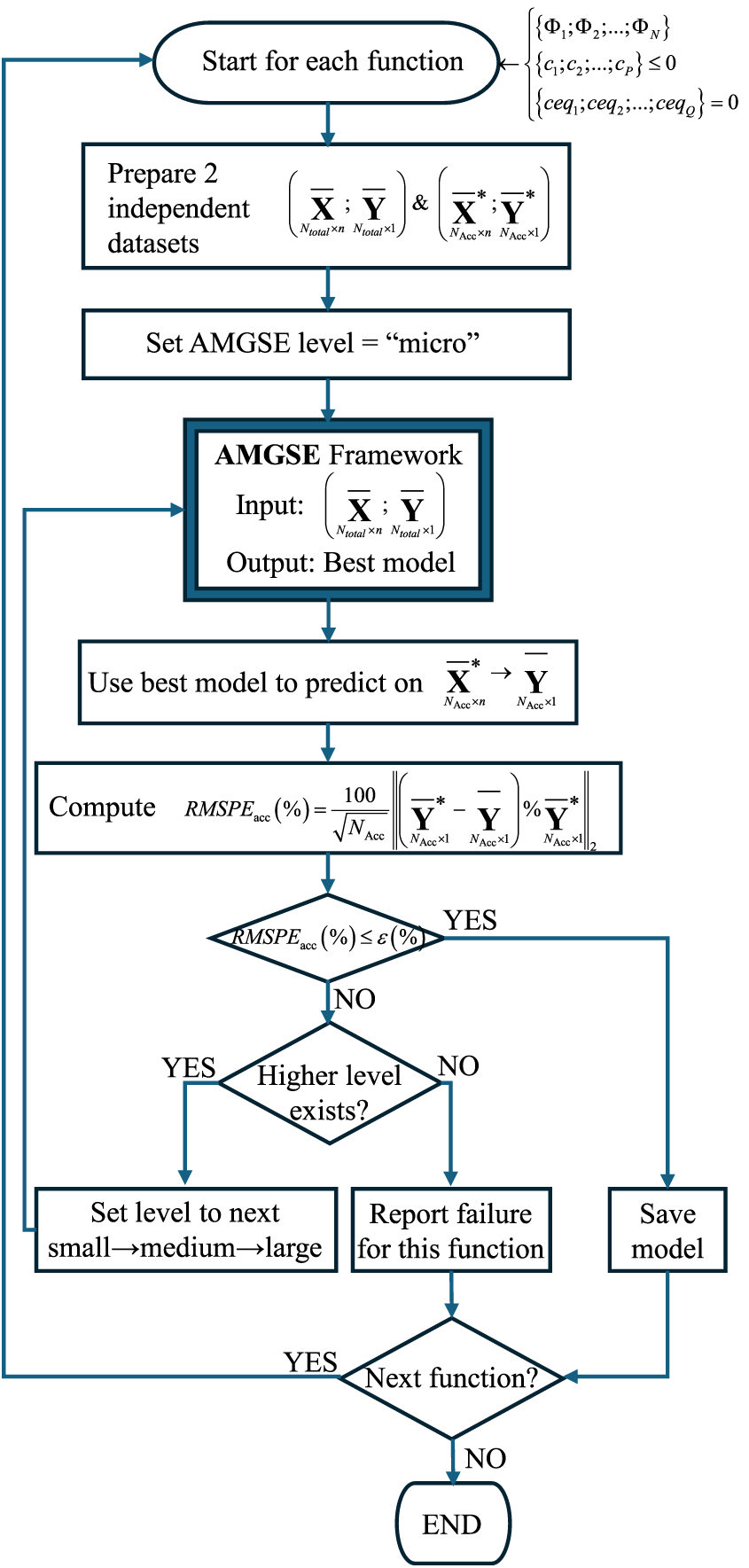
Figure 2: Flowchart of hierarchical AMGSE-based process for constructing ANN surrogate models of objective and constraint functions from experimental data.
The process starts by iterating sequentially over each objective or constraint function. For each function, two statistically independent datasets are prepared: (i) a training dataset {
For a given function, the AMGSE framework is first executed at the micro level, corresponding to the smallest model complexity and the least computational cost. Using only the training dataset {
The resulting ANN surrogate model is then evaluated on the external acceptance dataset {
Because of the 1/NAcc averaging factor the metric does not grow mechanically with the number of acceptance samples, and the relative formulation makes it invariant under a common non-zero rescaling of the response and of its prediction; it is therefore directly interpretable as a percentage and comparable across responses of different physical magnitudes. It presupposes true outputs bounded away from zero, and for responses that can vanish over the design domain a normalized root-mean-square error is used instead (Section 4.9). If the computed RMSPE (%) is smaller than or equal to a predefined tolerance threshold ε (%), the surrogate model is deemed sufficiently accurate and is accepted and saved as the mathematical representation of the corresponding objective or constraint function. The external acceptance set is used solely for the pass/fail decision between search levels. If escalation occurs, an additional untouched evaluation set is advisable for final generalization reporting.
If the accuracy requirement is not satisfied, the framework escalates the AMGSE execution to the next higher complexity level along the ordered ladder micro → small → medium → large; because execution starts at the micro level, the first escalation is to small, and the framework then proceeds to medium and to large as required. Each level corresponds to an increased model capacity and a broader hyperparameter search space, enabling the framework to capture more complex functional relationships when necessary. At each level, a new ANN surrogate model is constructed from the same training dataset {
If all AMGSE levels are exhausted without meeting the prescribed accuracy threshold, the framework reports a failure for the corresponding function, along with diagnostic information such as the best achieved RMSPE and potential causes (e.g., insufficient training data, high noise levels, strong nonlinearity, or inadequate input features). The process then proceeds to the next objective or constraint function.
This procedure is repeated until all objective and constraint functions {Φ1, Φ2, …, ΦN, c1, c2, …, cP, ceq1, ceq2, …, ceqQ} have been processed. The final outcome is a complete optimization model composed entirely of independently validated ANN surrogate functions, which can subsequently be employed in gradient-based or gradient-free optimization algorithms for efficient design exploration and decision-making.
3.2 Multi-Objective Optimization Using AMGSE-Based Surrogate Models with Real-Model Verification
Once all objective and constraint functions have been successfully approximated using validated AMGSE surrogate models, resulting in the model files model_fi.mat (i = 1, 2, …, N + P + Q)—the complete multi-objective optimization problem can be formulated as (Fig. 3):
where all functions
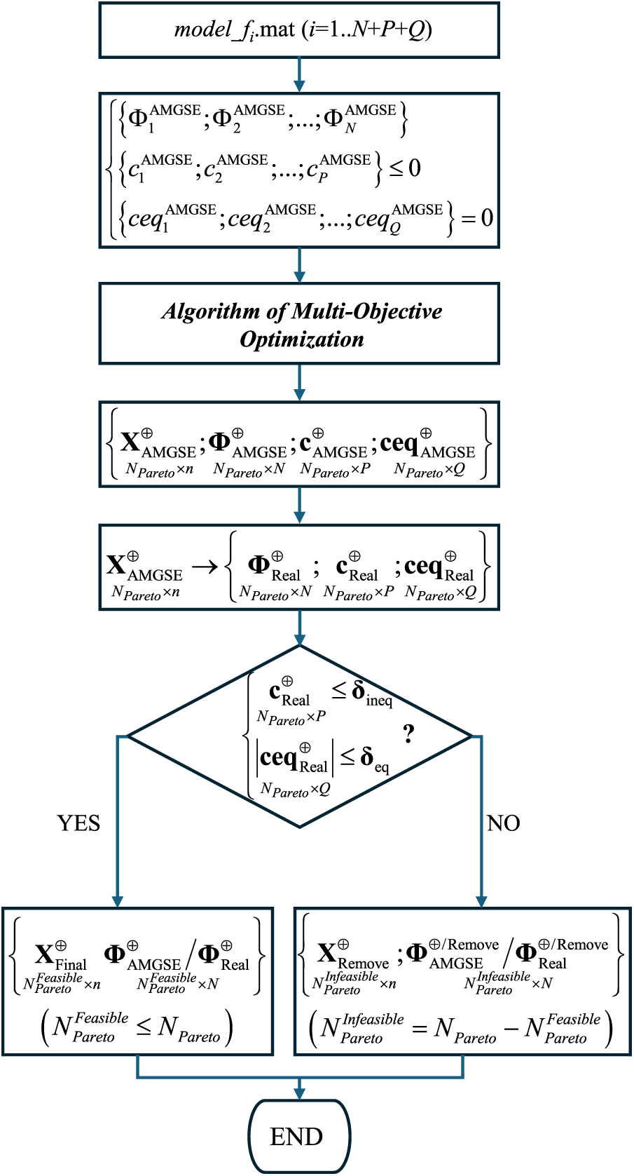
Figure 3: Flowchart of multi-objective optimization using AMGSE-based surrogate models with real-model verification.
Step 1: Surrogate-Based Pareto Front Generation
A multi-objective optimization algorithm (e.g., NSGA-II, NSGA-III, MOEA/D, or decomposition-based methods) is applied to the surrogate-model-based optimization problem. Because the surrogate models provide computationally inexpensive function evaluations, the algorithm can perform extensive exploration of the design space with minimal computational cost. This process yields a Pareto-optimal solution set denoted as:
where
Step 2: Real-Model Re-Evaluation
Although the surrogate models have been validated to satisfy
To ensure the reliability of the final Pareto front, every candidate solution
for
Important note on computational feasibility: In typical engineering multi-objective optimization scenarios, the number of Pareto-optimal solutions
Where exhaustive verification is impractical (very large Pareto sets, or extremely expensive single evaluations), a representative subset of the front can be verified instead; candidate subset-selection strategies are outlined in Supplementary Section S8.
Step 3: Feasibility Filtering Based on Real Constraints
Each solution is then checked against the real constraint values to determine its true feasibility:
where
– Feasible solutions are retained and constitute the exact-model-verified feasible candidate set:
where
– Infeasible solutions are discarded:
where
Exact-objective non-dominated re-sorting. Feasibility filtering alone does not establish Pareto optimality with respect to the exact models. Because the objective vector of every retained candidate is recomputed with the high-fidelity models, a solution that was non-dominated under the surrogate predictions may become dominated once the exact values are substituted. The retained set is therefore subjected to a non-dominated sorting under the exact objectives, and any dominated member is removed, before the result is reported as a Pareto set; duplicate objective vectors are identified at the same stage. Three quantities are consequently distinguished throughout this work: the surrogate-nondominated candidates returned by the optimizer, the subset of these that passes exact-model feasibility verification, and the exact non-dominated subset of that subset, which constitutes the final validated Pareto set reported to the decision-maker. In the present case study they number 152, 151 and 150, respectively, the last comprising 146 distinct objective vectors (Section 4.4).
Step 4: One-Pass Strategy and Potential Extensions
The framework presented here adopts a one-pass strategy, which was sufficient for the present case study: the multi-objective optimization algorithm is executed once using the surrogate models, and the resulting Pareto front is subsequently verified against the real models without further iteration. This approach is justified by the following considerations:
1. Surrogate model quality assurance: All AMGSE surrogate models have been accepted on their external acceptance datasets to ensure
2. Computational efficiency: The one-pass strategy minimizes the number of expensive real-model evaluations, which are performed only for the final candidate solutions rather than iteratively throughout the optimization process.
3. Practical applicability: When the verified feasible fraction is high, as in the present case study, the final validated Pareto set obtained from
An iterative optimization–verification extension is possible when the infeasible fraction of the front is unacceptably high; it is outlined in Supplementary Section S8 and is typically unnecessary when the surrogate models have been validated as described above.
The computational implications of this one-pass strategy (a single surrogate-based optimization pass followed by exact-model verification) for the present case study–including the realized training and verification costs–are quantified in Section 4.6.
4 Case Study: Multi-Objective Design of Slider–Crank Mechanisms with Springs
4.1 Mathematical Model Description of SCM with Springs
Application of the AMGSE Framework to Multi-Objective Optimization of Spring Placement and Stiffness in Slider-Crank Mechanisms. Details of the mathematical model for the slider-crank mechanism incorporating springs, with application to a wood-splitting machine, are presented in the publication [32] and Fig. 4:
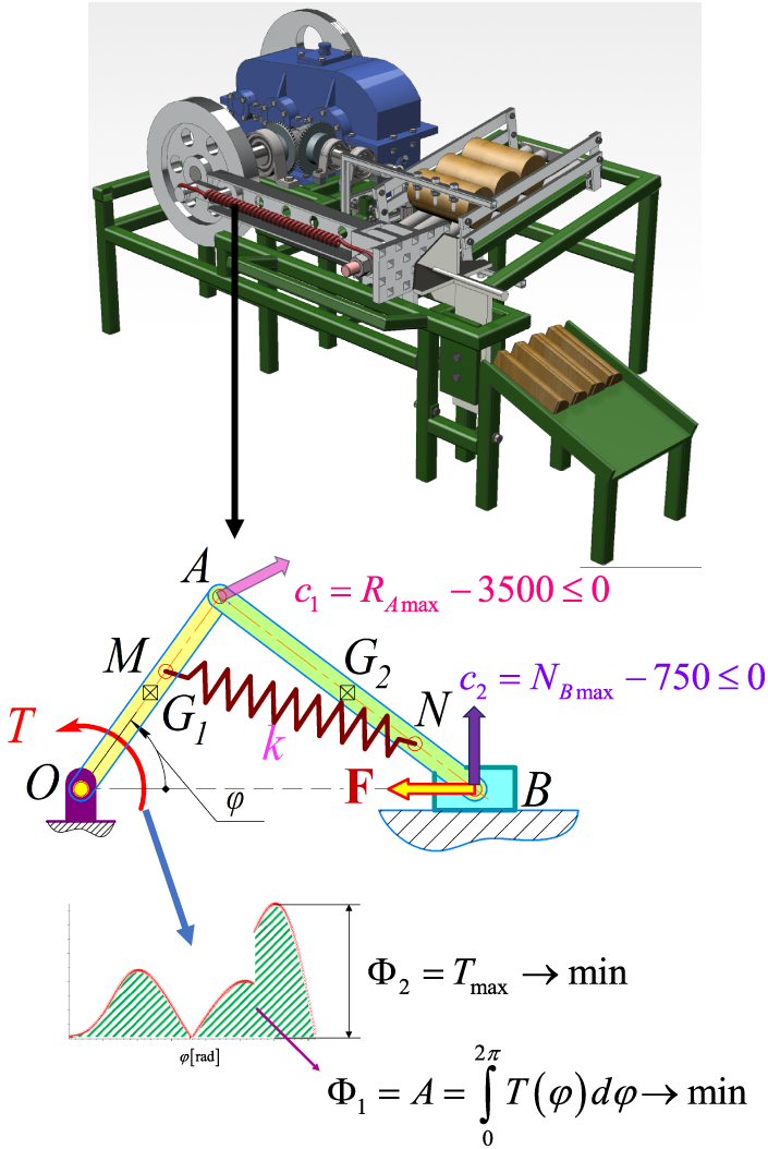
Figure 4: Mathematical model of the slider-crank mechanism with springs for wood-splitting machine application.
The mathematical model comprises two primary objective functions: the energy required to rotate the driving link through one full cycle (Φ1 = A → min) and the maximum torque during one rotation cycle of the driving link (Φ2 = Tmax → min). The two inequality constraints are that the maximum dynamic reaction force at joint A must not exceed 3500 N (c1 = RA,max − 3500 N ≤ 0) and the maximum reaction force from the groove on slider B must not exceed 750 N (c2 = NB,max − 750 N ≤ 0). The design variables for the problem are the parameters defining the positions of the spring attachment points M and N: α1 = OM/OA = 0…1; α2 = AN/AB = 0…1; and the spring stiffness k = 0…20,000 N/m.
4.2 Development of ANN-Based Surrogate Models Using the AMGSE Framework
Due to the relatively high computational time required to evaluate each function (RA,max, NB,max, Φ1, Φ2) for every design variable vector (α1, α2, k) (≈5 s), directly performing multi-objective optimization on this model would be excessively time-consuming and could result in an “endless computation” scenario. Therefore, we employ the AMGSE framework to train an equivalent surrogate model based on the primary dataset consisting of 2048 points from [32].
The training data, denoted as
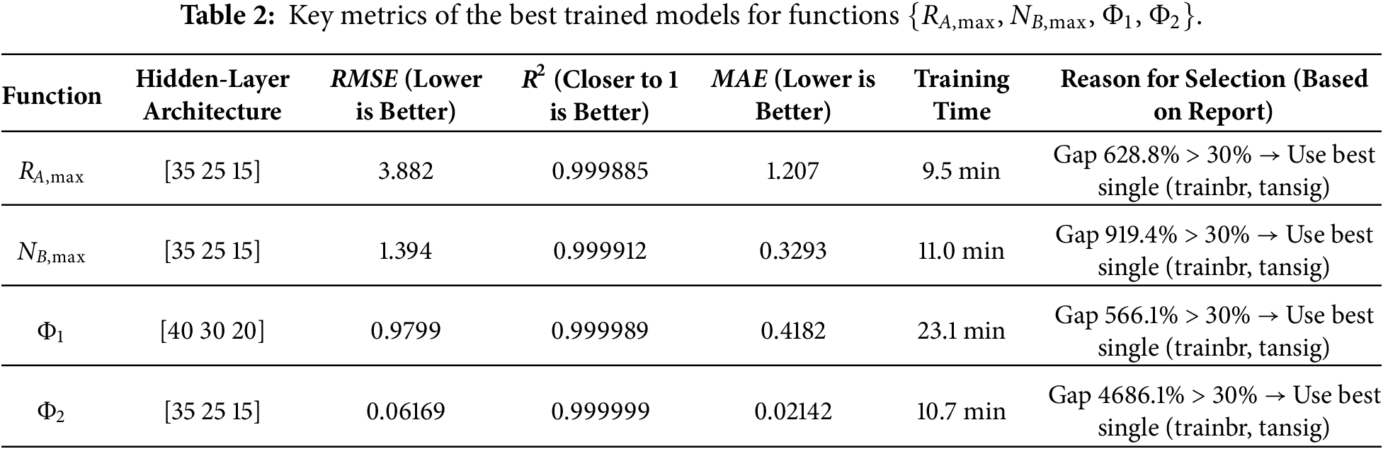
After applying the AMGSE framework to the four functions {RA,max, NB,max, Φ1, Φ2} the report indicates that, in all cases, the selection mechanism favors the best single surrogate rather than an ensemble, according to the AMGSE “gap” criterion (30% threshold). This outcome is reasonable for the present setting, which is essentially a deterministic dynamical system: once the parameters (α1, α2, k) are fixed, the input–output mapping follows stable, repeatable mechanical laws over cycles, while any noise in the available dataset is negligible. Consequently, the training data tend to reflect a smooth and consistent relationship, enabling an ANN to learn an accurate approximation; when a single model already achieves very small errors and an R2 value close to 1, the incremental benefit of ensembling is often limited because the individual models lack sufficient diversity, whereas the training and deployment cost may increase.
In contrast, for more complex multiphysics engineering problems–where data may involve noise, parameter uncertainty, or strongly nonlinear behavior that leads to high variability across training configurations–ensembles can be more advantageous, reducing predictive variance and improving generalization. A systematic investigation of ensemble benefits under such multiphysics scenarios is left for future work.
4.3 Validation of the Surrogate Models
4.3.1 Comparison with the High-Fidelity (Exact) Model
Throughout Sections 4.3–4.7, the 150-point external set denotes the independently generated dataset that was used once for the micro-level acceptance decision and subsequently for comparative evaluation; the errors reported on it are therefore acceptance-set rather than fully untouched post-selection estimates.
The trained models are re-evaluated using an assessment dataset of 150 design points, generated independently via Latin Hypercube Sampling over the full design domain and evaluated with the exact model of [32]; this set has zero overlap with the 2048-point training set (verified by nearest-neighbor distance). Specifically, the four selected models are employed to predict the values of the four functions. The relative errors between the predicted and actual function values at these 150 assessment points are illustrated in Fig. 5.
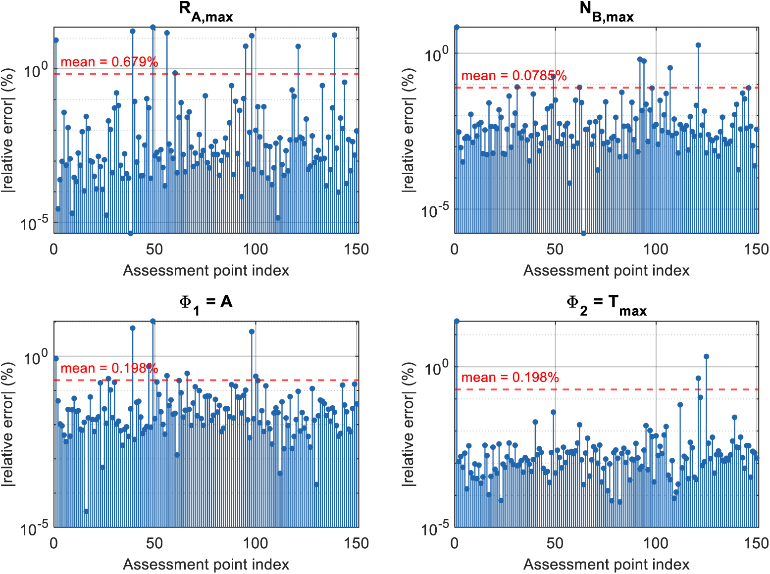
Figure 5: Percentage error between AMGSE-ANN predictions and exact model of functions RA,max, NB,max, Φ1, Φ2.
The RMSPE(%) values, aggregated from the error table for the 150-point assessment dataset for each function, are presented in Table 3. The RMSPE values in Table 3 are computed using the same prediction pipeline as the AMGSE ANN RMSPE column reported in Section 4.3.3 and are therefore consistent.

As shown in Fig. 5 and Table 3, the numerical results confirm the effectiveness of the AMGSE framework in automating architecture optimization and model selection, achieving RMSPE values between 0.59% and 3.11% across the four functions on the independent 150-point assessment set.
The equivalent AMGSE-ANN model is utilized to plot the graphs of the functions RA,max(α1, α2); NB,max(α1, α2); Φ1 = A(α1, α2); Φ2 = Tmax(α1, α2) and compare them with the graphs constructed from the accurate model in [32].
The comparative plots for the functions shown in Figs. 6–9 demonstrate that the equivalent models trained via the AMGSE Framework yield low average prediction error, producing response surfaces that are visually very close to those generated by the exact model, consistent with the 0.59%–3.11% RMSPE range reported in Table 3. Furthermore, the computational time required to generate plots from these equivalent models is approximately 71–85 times shorter (about 81× overall; for generating the complete response-surface plots; per-point inference takes milliseconds vs. ≈5 s per function for the exact model). This highlights the superior efficiency of surrogate models, provided that high training quality is achieved.
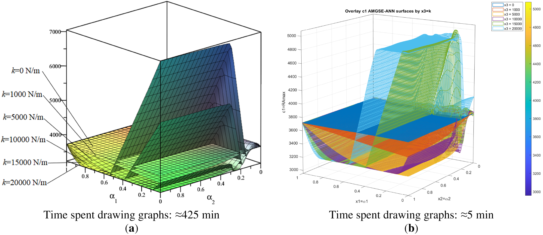
Figure 6: Overlay RA,max(α1, α2) surfaces by x3 = k; (a) exact model [32]; (b) AMGSE-ANN surrogate model.
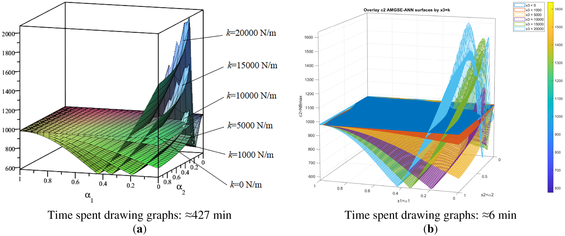
Figure 7: Overlay NB,max(α1, α2) surfaces by x3 = k; (a) exact model [32]; (b) AMGSE-ANN surrogate model.
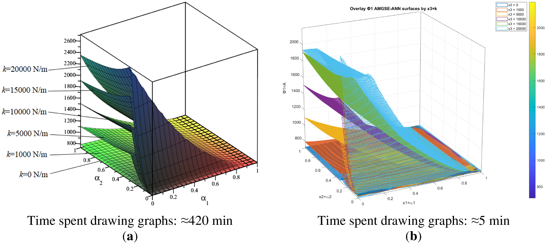
Figure 8: Overlay Φ1 = A(α1, α2) surfaces by x3 = k; (a) exact model [32]; (b) AMGSE-ANN surrogate model.
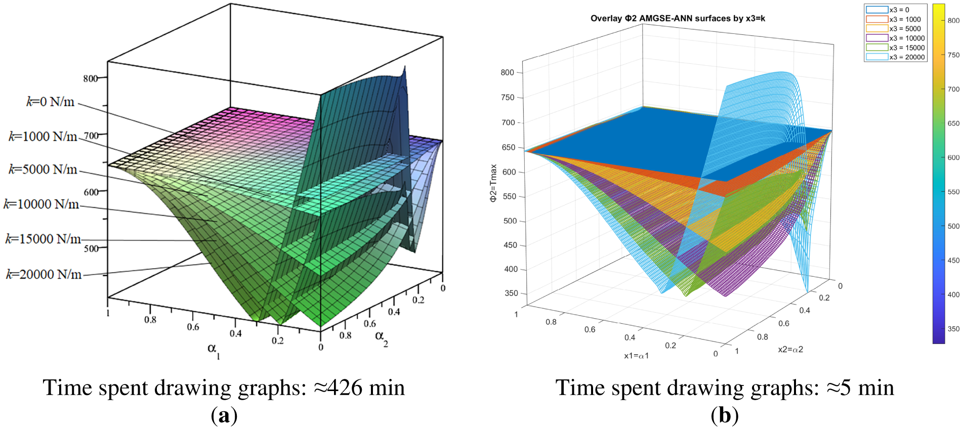
Figure 9: Overlay Φ2 = Tmax(α1, α2) surfaces by x3 = k; (a) exact model [32]; (b) AMGSE-ANN surrogate model.
4.3.2 Comparative Analysis with Hyperparameter-Optimization Baselines
This subsection compares strategies for selecting ANN hyperparameters: in all compared methods, the final surrogate remains an ANN, and the methods differ only in how its configuration is chosen. Claims in this subsection, therefore, concern hyperparameter optimization, not surrogate families; a comparison with fundamentally different surrogate models is provided in Section 4.3.3. We conduct a systematic comparison of prediction accuracy achieved by the AMGSE-trained models against three representative hyperparameter optimization baselines: Bayesian Optimization (BO), Tree-structured Parzen Estimator (TPE), and Random Search (RS). This comparative analysis evaluates all four methods using the same independent 150-point assessment dataset (Latin Hypercube Sampling, evaluated with the exact model of [32], with zero overlap with the training set), providing a common external evaluation basis without confounding factors from differences in data selection.
Experimental protocol and statistical evaluation. Because all compared algorithms are stochastic, the comparison was repeated over ten independent runs (seeds 101–110) per method and per function under a matched-conditions protocol: identical candidate architectures {[40, 30, 20], [35, 25, 15]}, training algorithms {trainlm, trainbr}, activation function {tansig}, data partition (70/20/10), and a common wall-clock ceiling of 900 s for the three baselines under each method’s own stopping protocol, while AMGSE executes its prescribed micro-scale protocol of 32 trainings; performance is measured as the mean absolute relative error over the 150-point independent assessment set. Table 4 reports the resulting statistics. AMGSE mean-error values for the full 2048-point design differ slightly between the ten-run campaign reported here and the values reported in Sections 4.3.3, 4.5 and 4.7.2 and in Supplementary Table S4, because the present campaign reports ten-run statistics, whereas those report, respectively, the single deployed surrogate, five-run ablation averages, and single reference runs executed with the seeds of their respective experiments. AMGSE achieves the lowest mean error on three of the four functions (NB,max, Φ1, Φ2), with margins of 3.3–10.6× in mean error over all three baselines (ratios computed from unrounded means), and is more accurate than TPE on the fourth function (RA,max); on RA,max, AMGSE is modestly outperformed by BO and RS (by approximately 25% in mean error). The Friedman test rejects the hypothesis of equal performance on every function (p < 5 × 10⁻⁵), and post-hoc Wilcoxon signed-rank tests against each baseline, with Holm correction, are significant in all twelve pairwise comparisons (p ≤ 7.8 × 10⁻³). Distribution plots are provided in Supplementary Fig. S1. Fig. 10 directly visualizes the ten-run campaign statistics from Table 4 (mean ± standard deviation across the ten seeds). Fig. 11 shows the spatial error pattern across the 150 assessment points for a single representative run (seed 101); aggregate run-to-run statistics are reported in Table 4 and Supplementary Fig. S1. For clarity, the data roles are as follows: the training split (70%) updates network weights; the validation split (20%) drives early stopping and restart selection; the internal selection split (10%; Xsel, Ysel in the Appendix C pseudocode) is used for configuration ranking and ensemble decisions; and the external 150-point assessment set, together with the 608 exact-model verification evaluations (152 designs × 4 responses), did not influence weight fitting, restart selection, configuration ranking or ensemble construction. It was used once, as an external acceptance set, to determine whether escalation beyond the micro level was required; because the tolerance was satisfied, the escalation branch was not triggered. Its reported errors should therefore be read as acceptance-set performance rather than as a fully untouched post-selection estimate.
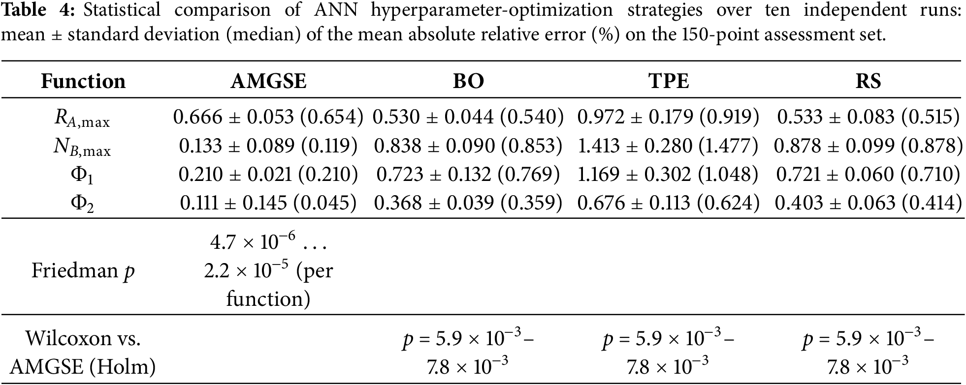
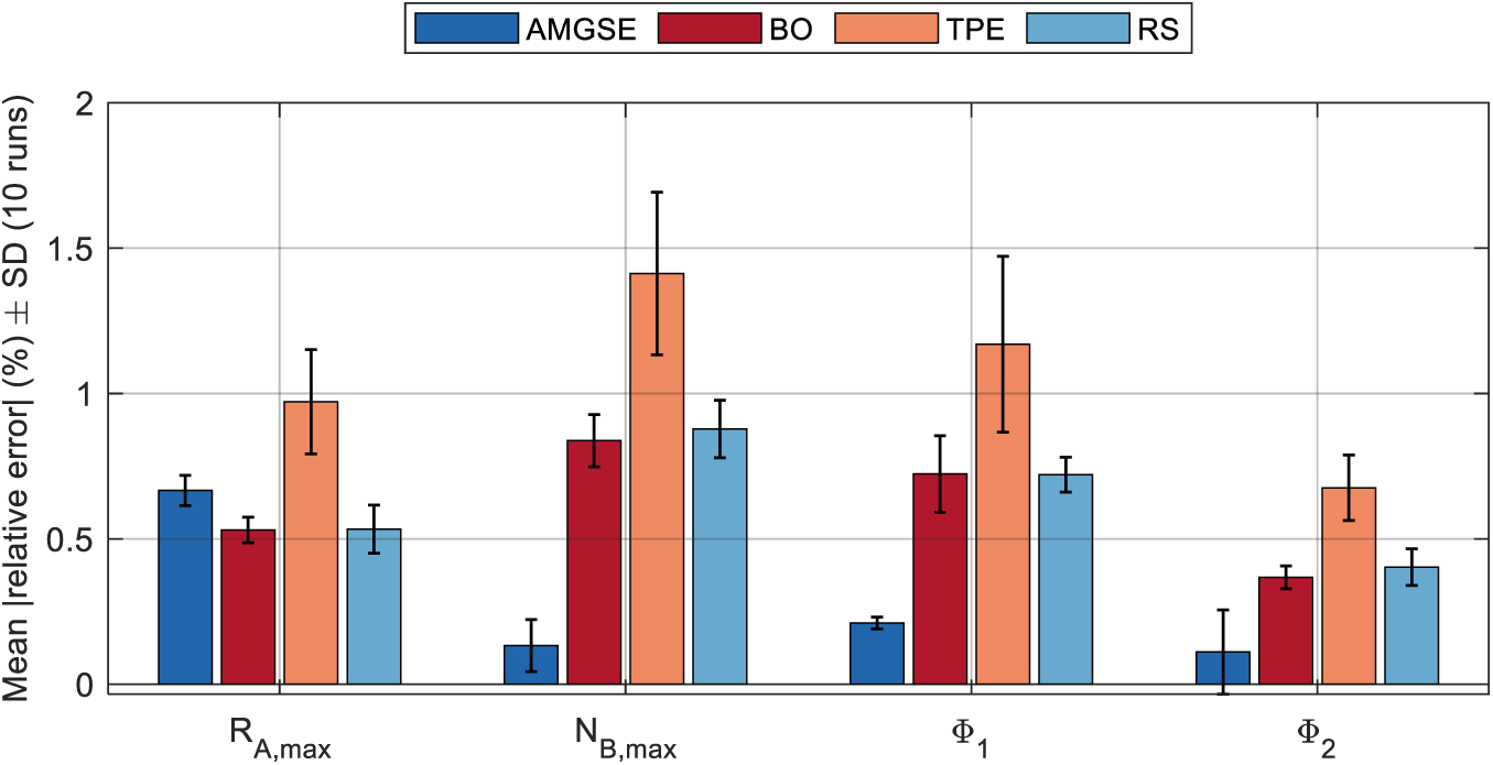
Figure 10: Prediction accuracy comparison across all objective and constraint functions (ten-run campaign statistics, mean ± standard deviation; see Table 4).
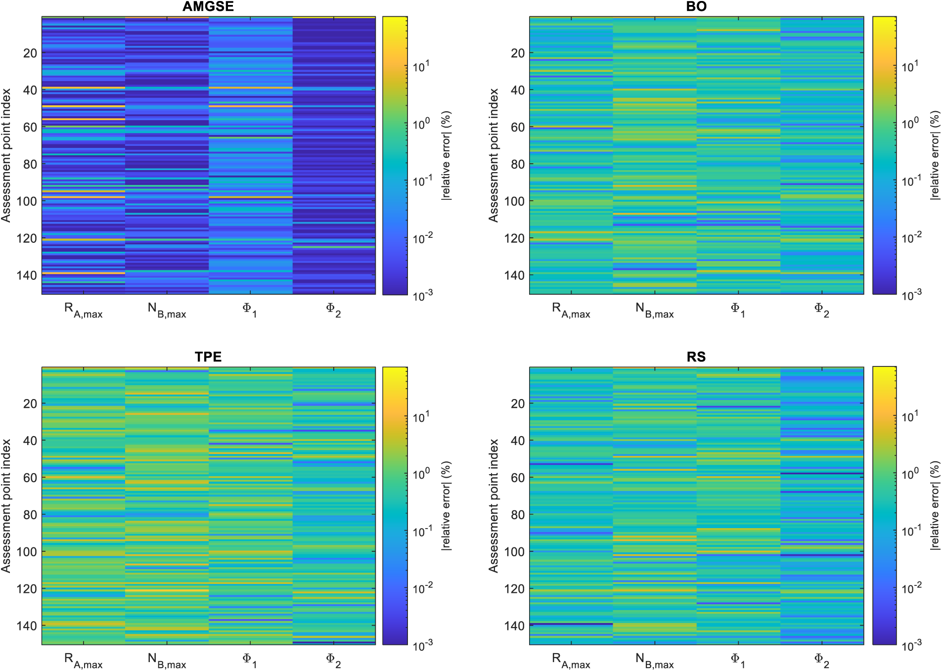
Figure 11: Spatial error distribution and model robustness.
Fig. 10 presents a quantitative comparison of mean prediction errors and their variability (depicted via error bars representing standard deviation) achieved by AMGSE and three competing methods across the four functions {RA,max, NB,max, Φ1, Φ2}. The analysis reveals AMGSE’s significantly superior predictive accuracy and consistency, attaining the lowest mean error on three of the four functions (NB,max, Φ1, Φ2), whereas its relative standing on RA,max is discussed below:
– AMGSE achieves mean errors (± standard deviation across ten seeds) of 0.666 ± 0.053% (RA,max), 0.133 ± 0.089% (NB,max), 0.210 ± 0.021% (Φ1), and 0.111 ± 0.145% (Φ2), attaining the lowest mean error among the four compared methods on NB,max, Φ1, and Φ2.
– Bayesian Optimization attains mean errors of 0.530% (RA,max), 0.838% (NB,max), 0.723% (Φ1), and 0.368% (Φ2). BO is 3.3–6.6× less accurate than AMGSE on NB,max, Φ1, and Φ2, but modestly more accurate than AMGSE on RA,max (0.530% vs. 0.666%, about 26% lower).
– Random Search attains mean errors of 0.533% (RA,max), 0.878% (NB,max), 0.721% (Φ1), and 0.403% (Φ2). RS is 3.3–6.6× less accurate than AMGSE on NB,max, Φ1, and Φ2, but modestly more accurate than AMGSE on RA,max (0.533% vs. 0.666%, about 25% lower), similarly to BO.
– TPE attains mean errors of 0.972% (RA,max), 1.413% (NB,max), 1.169% (Φ1), and 0.676% (Φ2), the least accurate of the three baselines on every function; AMGSE is 1.5–10.6× more accurate than TPE across all four functions.
Key observation: AMGSE attains the lowest mean error on three of the four functions (NB,max, Φ1, Φ2), by margins of 3.3–10.6× over all three baselines, and is more accurate than TPE on the fourth function (RA,max) while being modestly outperformed there by BO and RS. This pattern is consistent across all ten independent runs (Table 4; a large absolute rank-biserial effect size–equal to 1.0 in nine of the twelve significant pairwise comparisons and between 0.93 and 0.96 in the remaining three (RA,max vs. RS, and Φ2 vs. BO and RS), the sign indicating whether AMGSE or the corresponding baseline attained the lower paired error).
AMGSE’s advantage on three of the four functions is associated primarily with its systematic grid coverage and full-convergence training at the micro scale; the ablation study (Section 4.5) indicates that multi-restart selection adds little measurable mean-accuracy benefit in this deterministic case study (R = 8 restarts per configuration), which more thoroughly explores the fixed architecture-algorithm space than the stochastic search strategies of BO, TPE, and RS under their respective method-specific stopping protocols, with realized computational costs reported separately. On RA,max, however, AMGSE’s exhaustive search does not translate into better held-out accuracy than the more sparingly-sampled BO and RS baselines; a plausible explanation is a mild selection-induced optimism effect (an “optimizer’s curse”), whereby ranking many candidates by a noisy internal validation criterion increases the risk of selecting a configuration that is well matched to that split’s particular sampling noise rather than to the true underlying function–an effect naturally attenuated when fewer candidates are evaluated. In the present N = 2048 campaign, the adaptive complexity module is inactive (its activation threshold is 300 samples); its role is exercised separately in the small-sample stress test of Section 4.7.
Fig. 11 provides a heatmap comparing absolute prediction errors across all 150 assessment points for each method in a single representative run (seed 101); aggregate run-to-run statistics are reported in Table 4. All four methods exhibit a small number of design points with locally large errors, most likely corresponding to regions of the design domain that are sparsely represented in the 2048-point training set: for this run, the maximum pointwise error reaches 22.8% (AMGSE, RA,max), 29.0% (TPE, NB,max), and 71.5% (AMGSE, Φ2, a single isolated point), while the 90th-percentile error remains below 3% for every method and function. This indicates that, despite its mean-accuracy advantage on three of the four functions, AMGSE’s surrogate is not uniformly reliable across the full design domain, and occasional large local errors can occur for any of the four methods; this behavior is discussed further as a limitation in Section 4.8.
The comparative analysis in Figs. 10 and 11 shows that AMGSE delivers higher surrogate model quality on three of the four response functions–lower mean prediction error, consistent with the 3.3–10.6-fold differences reported in Table 4—compared to three established hyperparameter optimization alternatives. Although the AMGSE-trained surrogates attain the lowest mean error on three of the four functions, the spatial error analysis (Fig. 11) reveals occasional large local errors; the reported mean accuracy therefore reflects average rather than uniform pointwise reliability, and exact-model verification of the final Pareto candidates remains essential before subsequent design-space visualization and multi-objective optimization.
Building upon these results, a rigorous validation process was conducted for each surrogate function, including error-plot analysis, RMSPE (%) evaluation, and graphical comparison with the exact model. The results consistently demonstrate that the AMGSE-based surrogate models achieve low average error on the external assessment set, although the occasional large local errors in Fig. 11 preclude claims of uniformly reliable point-wise accuracy. Consequently, these validated models provide a solid foundation for subsequent multi-objective optimization and can be applied to the class of problems studied here, while retaining exact-model verification for all final optimization candidates.
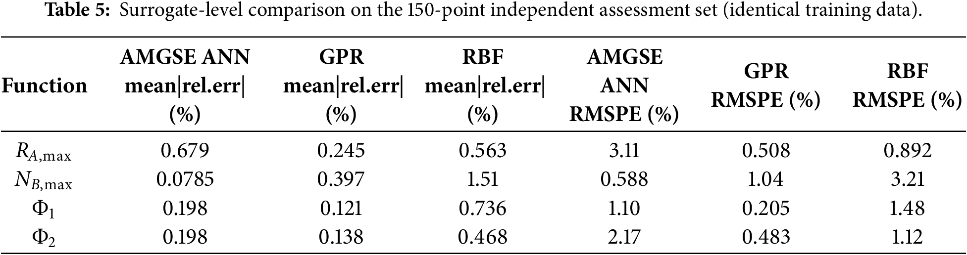
4.3.3 Surrogate-Level Comparison with Gaussian Process Regression and RBF Networks
The comparison in Section 4.3.2 concerns hyperparameter-optimization strategies for ANNs. To assess AMGSE at the surrogate level, the AMGSE-selected ANN is further compared against two fundamentally different surrogate families trained on the identical 2048-point dataset and evaluated on the identical 150-point independent assessment set: Gaussian Process Regression (GPR/Kriging) with automatic kernel selection over squared-exponential, Matérn and rational-quadratic families including ARD variants, automatic basis-function selection (constant, linear, pure quadratic), 5-fold cross-validation and multi-restart hyperparameter fitting; and Radial Basis Function (RBF) networks with a systematic sweep over spread and error-goal parameters. Table 5 summarizes the results. To match the statistical rigor of the ten-run hyperparameter-optimization campaign, 95% bootstrap confidence intervals (10,000 resamples) and paired Wilcoxon signed-rank tests on the point-wise absolute relative errors were computed on the 150-point set: every AMGSE-ANN-vs-GPR and AMGSE-ANN-vs-RBF difference is statistically significant (Holm-corrected p < 10−10). Although GPR attains the lower mean on three functions, the AMGSE ANN attains the lower median point-wise error on all four, with a larger mean arising from a heavier tail of a few large local errors (consistent with Fig. 11); the full confidence intervals are listed in Supplementary Section S10. GPR attains the lowest mean absolute relative error on three of the four functions (RA,max, Φ1, Φ2), outperforming the AMGSE ANN by 2.8× on RA,max, 1.6× on Φ1, and 1.4× on Φ2; the AMGSE ANN attains the lowest error on the remaining function, NB,max, outperforming GPR by 5.1× and RBF by 19.2×. RBF is the least accurate family among NB,max, Φ1, and Φ2, but modestly outperforms the ANN on RA,max (1.2×). Training cost is comparable across the three families (AMGSE ANN ≈ 39 min on average vs. 38–65 min for the tuned GPR and RBF sweeps). GPR’s strong showing on three of the four functions is consistent with the well-documented strength of Kriging on smooth, low-dimensional (here, three-variable) response surfaces; however, its cubic training complexity in the number of samples limits scalability to larger datasets, whereas the ANN surrogate additionally provides millisecond-level batch inference used by NSGA-III in Section 4.4 (a dedicated benchmark measured 10–28 ms for the ANN vs. 3.2–34 s for GPR and 4.0–44 s for RBF over batches of 1000–10,000 points–two to three orders of magnitude faster; Supplementary Section S10), and remains the most accurate family on NB,max.
4.4 Multi-Objective Optimization of the Slider–Crank Mechanism Using the Developed Surrogate Models
The multi-objective optimization problem is solved using the surrogate models trained via the AMGSE Framework. The mathematical model is formulated as follows:
The constrained bi-objective optimization problem is solved using the Non-dominated Sorting Genetic Algorithm III (NSGA-III) [35,36] which extends the classical NSGA-II [37] by incorporating a reference-point-based selection mechanism to maintain solution diversity along the Pareto front.
NSGA-III employs uniformly distributed reference points, generated using the Das-Dennis approach [38], to guide the search toward well-distributed Pareto-optimal solutions. The algorithm follows an elitist evolutionary framework in which, at each generation, offspring solutions are created using binary tournament selection, simulated binary crossover (SBX), and polynomial mutation. The combined parent-offspring population undergoes constrained non-dominated sorting, where Deb’s constrained-dominance principle ensures that feasible solutions are always preferred over infeasible ones [37].
Survival selection fills the next generation by first including complete non-dominated fronts, then applying a niching mechanism based on reference-point association to select the remaining individuals from the critical front. This mechanism prioritizes reference points with fewer associated solutions, ensuring balanced coverage of the objective space.
Although NSGA-III was originally designed for many-objective problems (N ≥ 3), its systematic diversity preservation offers advantages for bi-objective problems, particularly in maintaining uniformly distributed solutions along the Pareto front.
Upon applying the NSGA-III algorithm, a set of 152 non-dominated candidate solutions was obtained.
By substituting the obtained optimal parameter set
Upon verifying the constraint conditions
Fig. 12 presents a comparative analysis of Pareto fronts obtained from three multi-objective optimization approaches applied to the slider-crank mechanism problem: the hybrid CDOS-PSI method [32], the ANN_NSGAIII surrogate model trained via the AMGSE Framework, and the NSGAIII_Real validation using the exact mathematical model. The pink squares represent 19 Pareto solutions from CDOS-PSI, while the blue circles denote 152 solutions from ANN_NSGAIII. The green-filled triangles correspond to 151 feasible solutions from NSGAIII_Real, satisfying constraints c1 ≤ 0 and c2 ≤ 0, with one infeasible point (gray hollow triangle, solution #64) violating c2. Selected solutions are highlighted as blue and orange eight-pointed stars for CDOS-PSI and NSGAIII_Real, respectively.
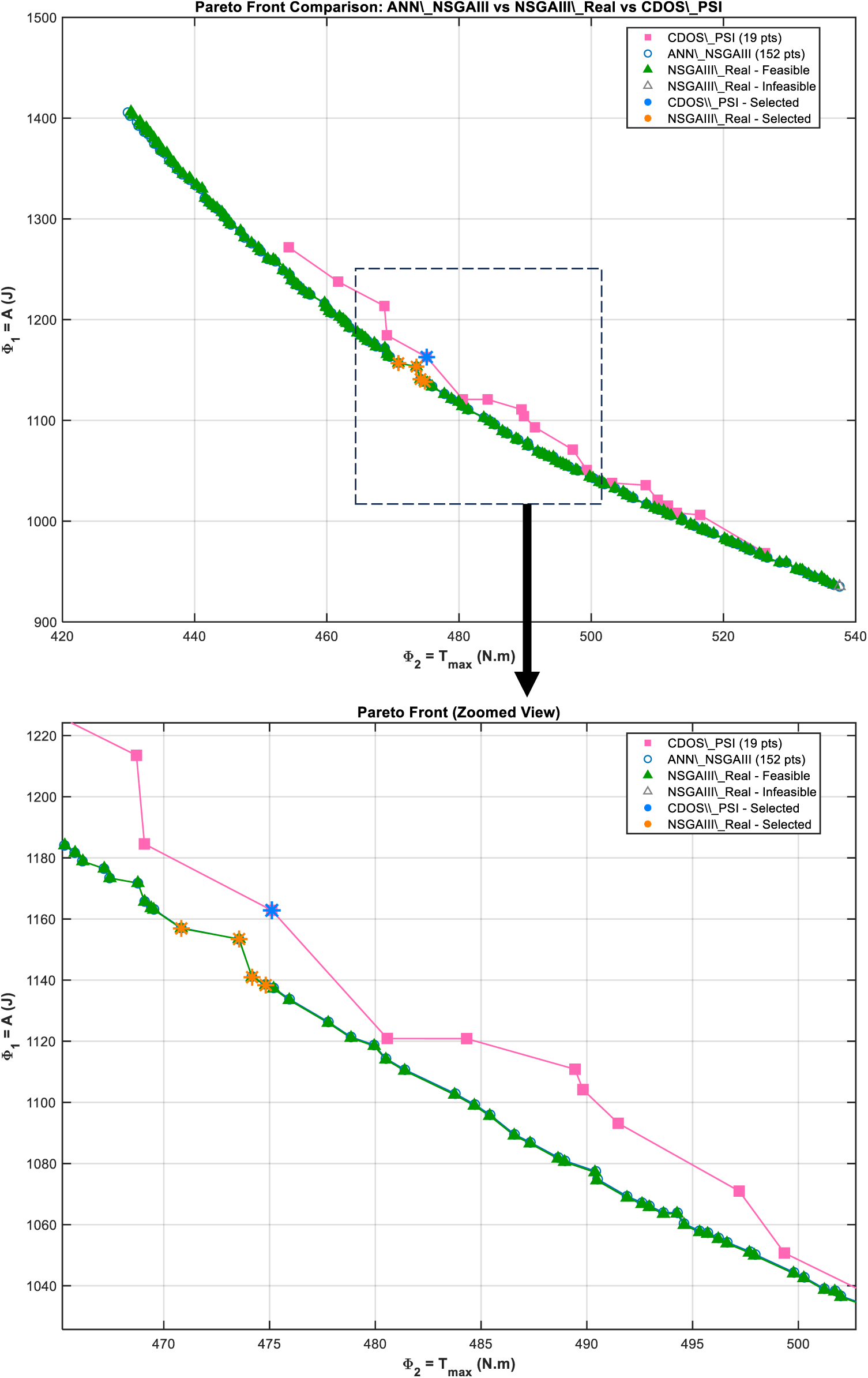
Figure 12: Pareto front comparison: ANN_NSGAIII vs. NSGAIII_Real vs. CDOS_PSI methods.
Notably, the ANN_NSGAIII and NSGAIII_Real solution sets exhibit close alignment, with 151 out of 152 ANN-derived solutions validated as feasible through exact computation, underscoring the high fidelity of the AMGSE-trained surrogate model in approximating the true objective space. This congruence validates the AMGSE Framework’s efficacy in generating accurate neural network surrogates for complex dynamics.
In comparison, the exact-model-verified feasible candidate set (NSGAIII_Real) contains substantially more solutions than CDOS-PSI, 151 against 19, and its exact non-dominated subset, referred to below as the exact-model-verified front, contains 150 of them. That front consistently dominates the CDOS-PSI front, lying entirely below in the objective space (Φ1 = A (J) vs. Φ2 = Tmax (N·m)). This dominance indicates enhanced trade-offs between minimizing A and minimizing Tmax, attributed to NSGA-III’s reference-point-based niching, which promotes diversity and convergence even in bi-objective scenarios.
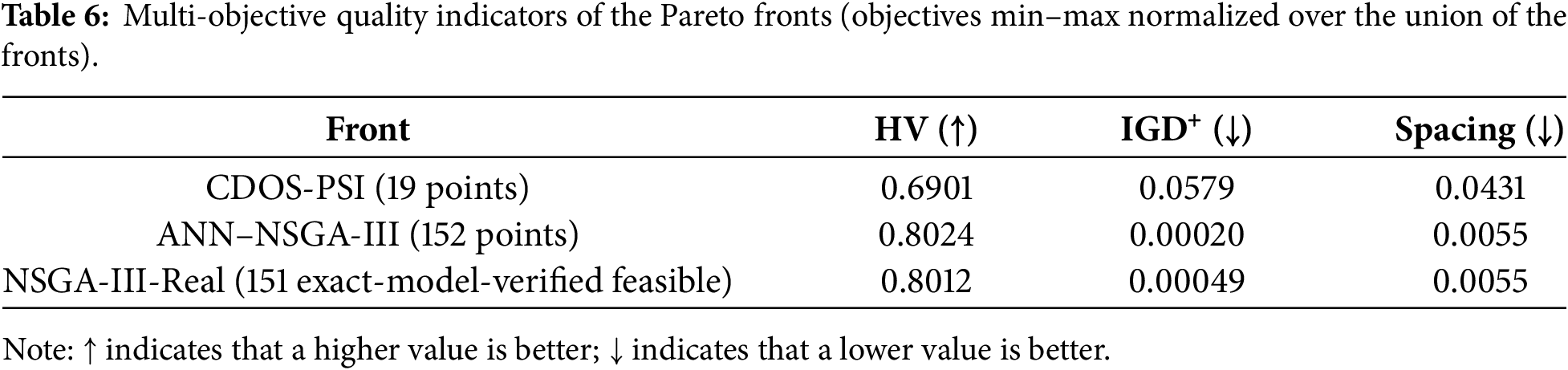
Quantitative Pareto-front assessment. To complement the visual comparison, three standard multi-objective quality indicators were computed on objectives normalized to [0, 1] over the union of the three fronts: the Hypervolume (HV, reference point (1.1, 1.1); higher is better), the Inverted Generational Distance Plus (IGD+, a dominance-compliant variant of IGD; reference set = non-dominated union front, 181 points; lower is better), and Schott’s Spacing (lower means a more uniform distribution). As summarized in Table 6, the ANN–NSGA-III front improves the hypervolume by 16.3% over CDOS-PSI (0.8024 vs. 0.6901)–and the exact-model-verified front improves it by 16.1% (0.8012 vs. 0.6901), the value quoted in the abstract and in contribution C4–reduces IGD+ by two orders of magnitude (2.0 × 10⁻⁴ vs. 5.8 × 10⁻²), and reduces Spacing by a factor of 7.9 (0.0055 vs. 0.0431), quantitatively confirming superior convergence, coverage, and uniformity. Moreover, the exact-model-verified front is nearly indistinguishable from the surrogate-predicted front (HV 0.8012 vs. 0.8024; IGD+ 4.9 × 10⁻⁴ vs. 2.0 × 10⁻⁴; Spacing 0.0055 for both), independently corroborating the fidelity of the AMGSE surrogates at the level of the final Pareto set. Because this comparison contrasts the complete AMGSE–NSGA-III pipeline with the previously reported CDOS-PSI solutions, the indicator gains are attributable to the pipeline as a whole rather than to any single component; the reported indicators were further confirmed to be robust to optimizer stochasticity: across ten independent NSGA-III runs the AMGSE–NSGA-III front was highly stable (median hypervolume 0.805, interquartile range 0.805–0.806, computed over the union of the ten runs and the CDOS-PSI front) and dominated the CDOS-PSI front in all ten runs, with every indicator significantly better than CDOS-PSI (Wilcoxon signed-rank test, p = 2.0 × 10⁻³, the smallest value attainable for ten paired runs and hence unanimous); each run returned 152 candidates, of which a median of 150 were mutually non-dominated on the surrogate front, whereas all 152 were mutually non-dominated in the representative run retained for exact-model verification. The point-wise quality of the representative front reported in Table 6 was certified by exact re-evaluation, and the union-based IGD+ reference naturally favors denser fronts. Recomputing the three indicators on the 150 mutually non-dominated exact solutions (146 distinct objective vectors) leaves HV, IGD+, and Spacing unchanged to the reported precision, because the single exact-dominated candidate lies within the front and Fig. 12 is unaffected. These evaluation caveats are acknowledged in Section 4.8.
Overall, these results highlight the AMGSE Framework’s potential for surrogate-based multi-objective optimization within the studied problem class, enabling rapid design-space exploration with modest computational overhead while preserving solution integrity through exact-model verification.
Among the 151 verified feasible solutions (150 mutually non-dominated), four solutions representing the best balance between the two objectives–specifically #44, #60, #70, and #142–are selected and presented in Table 7:
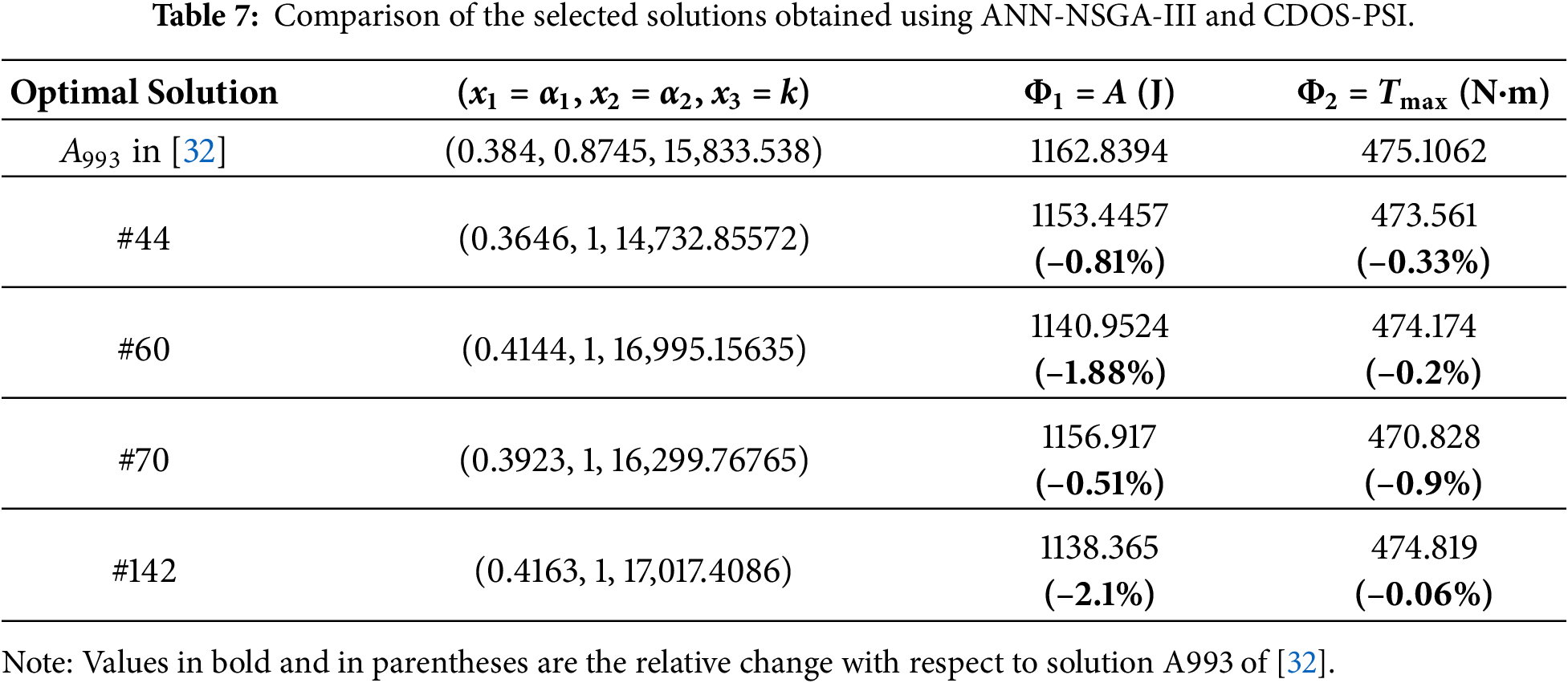
Based on Fig. 12 and Table 7, the four solutions selected via the proposed approach–utilizing the AMGSE framework for ANN training combined with the NSGA-III algorithm–exhibit superior quality compared to those obtained by the hybrid CDOS-PSI method. In terms of Pareto dominance, every solution of the CDOS-PSI front is dominated by at least one solution of the exact-model-verified front (19 of 19 points), while none of the 151 verified solutions is dominated by any CDOS-PSI solution; the same relations hold for the surrogate-predicted front.
4.5 Ablation Study of the AMGSE Modules
To quantify the contribution of the individual AMGSE modules, four variants were executed on identical data with identical seeds (five independent runs each; fewer than the ten of Section 4.3.2, as the run-to-run variance of the ablation variants proved comparatively small): (V1) the full framework; (V2) no multi-restart (R = 1); (V3) the 30% gap rule disabled, so that the ensemble is always eligible while the final ensemble-vs-single acceptance test of Phase 5 remains active; and (V4) ensembling disabled entirely. Table 8 reports the mean absolute relative error on the 150-point independent assessment set. On RA,max, NB,max, and Φ1, removing the multi-restart mechanism (V2) or disabling the gap rule (V3) changes the mean error by only a few percent relative to V1, well within one run-to-run standard deviation, indicating no material difference on these three functions. On Φ2, V2 and V3 both outperform V1 (0.091% and 0.200%, respectively, vs. 0.224% for V1); rather than degrading performance, disabling either mechanism modestly improved held-out accuracy for this function. This pattern differs from what would be expected if multi-restart selection and the gap rule reliably improved generalization, and is consistent with a mild selection-induced optimism effect: ranking more candidate models by a single internal validation split can occasionally favor a configuration that fits that split’s particular sampling noise slightly better without a corresponding gain in true generalization. Variant V4 coincides exactly with V1 on all four functions, because the gap criterion consistently favors the best single model in this deterministic, low-noise case study, so disabling ensembling has no effect by construction. Because the case-study dataset (N = 2048) exceeds the 300-sample activation threshold, the adaptive complexity module is not triggered here; its role is assessed separately in the small-sample experiment of Section 4.7. Fig. 13 visualizes these results. We further note that variant V2–one training per configuration over the same grid–is equivalent in practice to a single-restart grid-search baseline under the present implementation; even at this reduced cost (four single-shot trainings, on the order of the baselines’ realized costs in Table 9), it retains AMGSE’s advantage over BO, TPE, and RS on NB,max, Φ1, and Φ2, and its accuracy on RA,max remains close to that of V1 (both similar to BO and RS on this function). Overall, the ablation results indicate that the largest, most consistent contributor to AMGSE’s accuracy on this case study is the systematic grid coverage at the micro scale itself, rather than the multi-restart or conditional-ensemble mechanisms individually; the latter two provide a safety margin against poor initializations and heterogeneous candidate quality without an accuracy cost resolvable at five runs–the largest observed difference, on Φ2, lies within one run-to-run standard deviation–but do not appear to be the primary drivers of the accuracy advantage over BO/TPE/RS observed in Table 4.
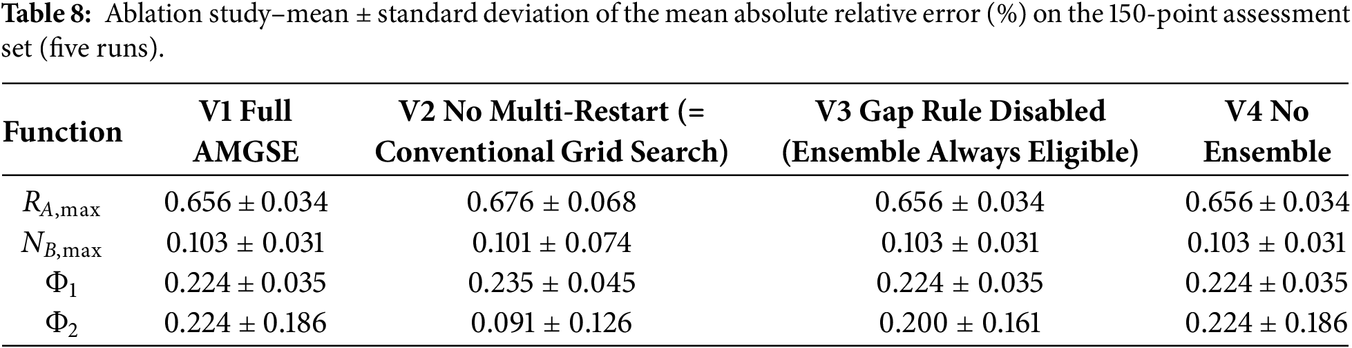
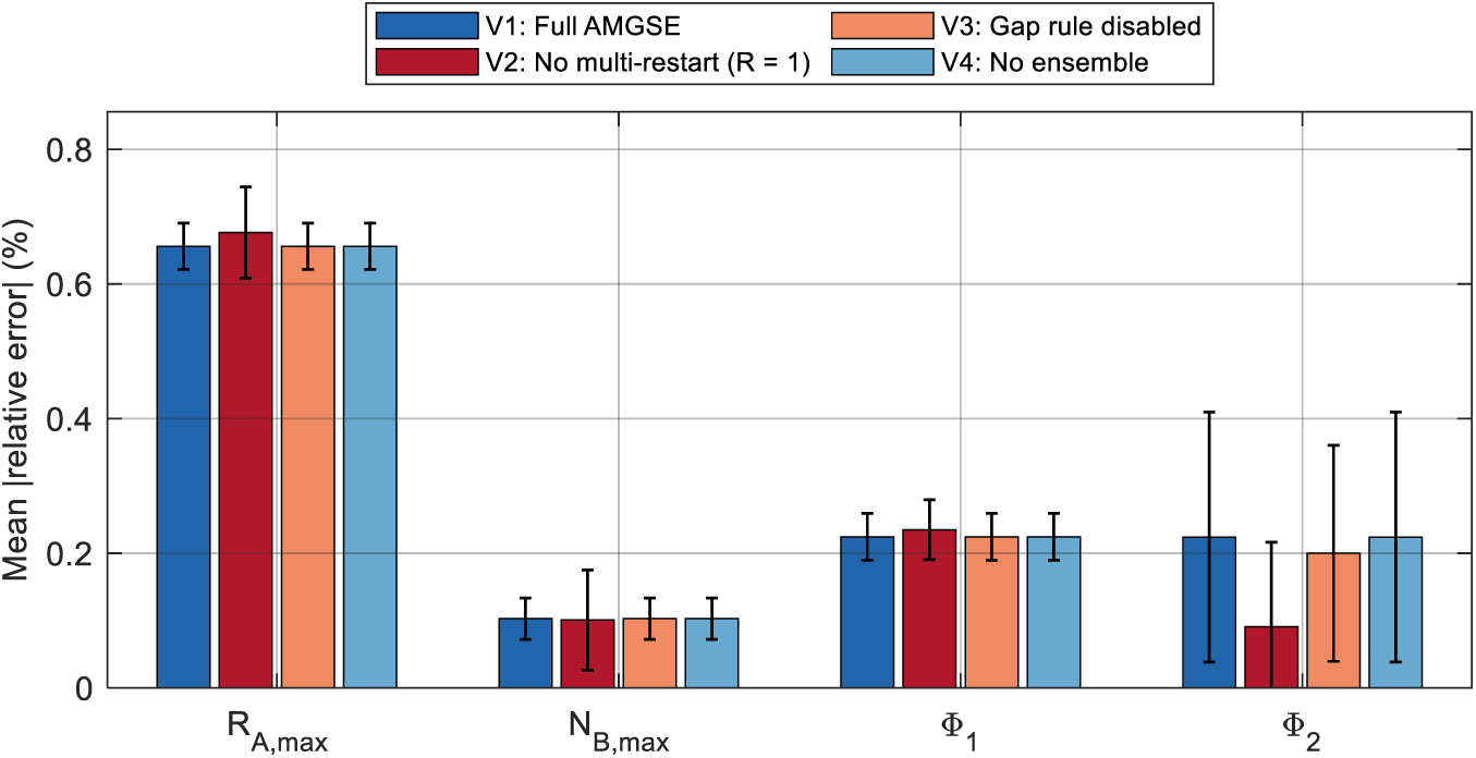
Figure 13: Ablation study–mean absolute relative error (%) on the 150-point assessment set (mean ± standard deviation over five runs).
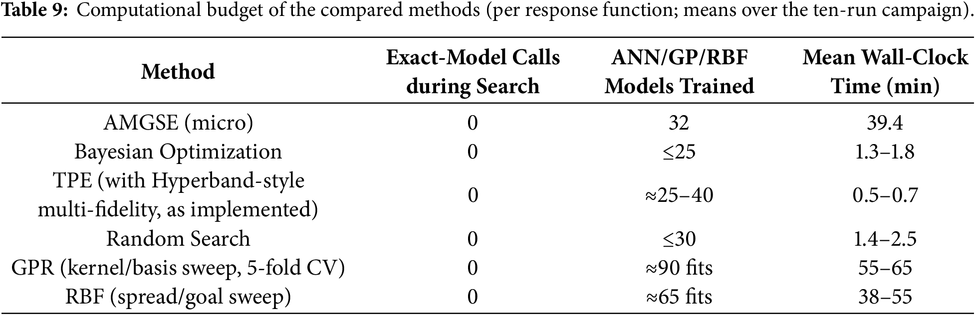
4.6 Computational Cost Analysis
4.6.1 Budget Accounting and Matched-Evaluation Check
A recurring concern with multi-layer search strategies is computational expense. It is essential to distinguish between the two budgets. The simulation budget–evaluations of the expensive exact model–is fixed and identical for all surrogate approaches: the 2048 offline samples inherited from [32] plus the verification of the 152 candidate designs (152 × 4 = 608 function evaluations); AMGSE performs no additional exact-model evaluations during its search. The training budget is the cost of fitting ANN candidates to the fixed dataset: at the micro scale, 4 configurations × 8 restarts = 32 training runs per function, requiring 39.4 min on average per function in our campaign (mean over 10 runs; hardware as in Section 4.2). The shorter per-function times in Table 2 (9.5–23.1 min) correspond to the single original deployed run executed under different machine-load conditions, whereas Table 9 reports campaign means on the current hardware. Under this matched-conditions protocol the baselines terminated at their own recommended stopping criteria after training a comparable number of models (25–30) in 0.5–2.5 min; their errors in Table 4 are thus obtained at a lower realized training cost; the corresponding budget question is addressed quantitatively both by the single-shot grid-search variant V2 of the ablation study (Section 4.5) and, more directly, by a matched-evaluation sanity check reported below. The tuned GPR and RBF sweeps of Section 4.3.3 required 38–65 min per function, comparable to AMGSE. For CFD-class applications, the dominant cost is data generation, which is common to all methods; AMGSE adds a training overhead of minutes to hours, negligible relative to typical simulation campaigns. When training a single ANN becomes expensive (e.g., due to very large datasets or architectures), the grid-with-restarts strategy becomes costly; this limitation is acknowledged in Section 4.8.
As an additional, more direct sanity check on the fairness of the comparison in Table 4, a matched-evaluation experiment was performed on two representative response quantities–Φ1 (the objective on which AMGSE shows its largest margin over the baselines) and RA,max (one of the two quantities on which the baselines attain the lowest mean error in Table 4)–over five independent seeds, evaluated on the 150-point independent assessment set. Two matched settings were compared: AMGSE run at its minimum realizable cost (Restarts = 1, four trainings, one-eighth of its default micro-scale budget of 32) against the baselines constrained to a comparable number of model fits (Bayesian optimization and random search capped at 32 evaluations; TPE bounded to its native 300-s stopping criterion). On Φ1, minimum-cost AMGSE attained a substantially lower mean absolute relative error (0.21%) than Bayesian optimization (0.78%), TPE (1.17%), and random search (0.76%), even though the latter trained up to eight times as many models, indicating that AMGSE’s advantage on this function is not an artifact of a larger training budget. On RA,max, the picture is mixed: the equal-fit-count random search (0.57%) and Bayesian optimization (0.61%) were marginally more accurate than minimum-cost AMGSE (0.71%), while TPE remained less accurate (1.01%)–a pattern consistent with the function-dependent trade-off already noted in Section 4.3.3, where the comparably inexpensive GPR surrogate attains the lowest mean error on three of the four response functions. Full per-method statistics are given in Supplementary Section S10.4.
4.6.2 Hierarchical Escalation Vs. a Flat Simultaneous Search
Because all four responses of the case study were accepted at the micro level, the escalation mechanism itself was not exercised there, and the argument of Section 2.2 would otherwise rest on analysis alone. We therefore re-ran the surrogate construction for Φ1 in flat mode, searching the medium space directly–20 configurations against the 4 of the micro level, that is 160 trainings against 32–on the identical dataset, data partition and restart budget, and evaluated the result on the same 150-point independent assessment set. The hierarchical arm reuses the micro-scale models already trained for the ten-run campaign in Section 4.3.2 (seeds 101–110), re-evaluating them on the same set without retraining. Table 10 reports the comparison. The medium space shares one of the two microarchitectures but does not contain the other, so the comparison is framed as a fivefold larger configuration space rather than a superset relation.

A fivefold increase in the number of training sessions reduced the assessment error from 0.2104 ± 0.0206% to 0.1889%, a relative improvement of about ten percent that places the flat result at the lower edge of the run-to-run band of the hierarchical arm (mean minus one standard deviation is 0.1898%). The individual hierarchical runs were 0.1805%, 0.1891%, 0.1911%, 0.1971%, 0.2060%, 0.2135%, 0.2274%, 0.2285%, 0.2330% and 0.2379%: one of the ten micro-scale runs was in fact more accurate than the fivefold more expensive flat search, and a second matched it to three significant figures. We deliberately report this comparison as a difference relative to run-to-run variability, in the same manner as the ablation study in Section 4.5, and do not attach a p-value to it: with a single flat run, a paired rank test has no power. Cost is reported as the number of trainings because that quantity is independent of hardware and of any interruption of the run. The corresponding comparison on an analytic benchmark, for which three independent flat runs were feasible, is reported in Section 4.9 and points in the same direction. The seed of the flat run and the full composition of the medium configuration space are given in Supplementary Section S11.
4.7 Behavior in the Small-Sample Regime
Experimental research often permits only 15–30 physical experiments. Although AMGSE targets the offline setting with moderate-sized datasets, its behavior under extreme data scarcity was examined by drawing a random 30-sample subset of the case-study data (fixed seed) and repeating surrogate construction. With N = 30 < 300 the adaptive complexity module activates automatically, scaling all layer widths by 0.7 (minimum eight neurons). Table 11 summarizes the errors on the 150-point independent assessment set. As expected, accuracy degrades markedly relative to N = 2048; the framework nevertheless remains operational without catastrophic overfitting. The comparison with GPR at N = 30 is mixed rather than uniformly favoring either family: the ANN is more accurate on NB,max (9.04% vs. 10.2%) and Φ2 (2.29% vs. 2.82%), while GPR is more accurate on RA,max (3.49% vs. 5.87%) and marginally more accurate on Φ1 (5.39% vs. 5.49%). We therefore explicitly note that Gaussian-process surrogates remain a competitive, and sometimes preferable, choice in the extremely small-sample regime, and that sequential model-based approaches with active sampling are more appropriate when the experimental budget itself is the binding constraint; integrating such adaptive sampling into AMGSE is identified as future work. Fig. 14 contrasts the three settings, making the operating envelope of the framework explicit. The N = 30 experiment is intended as an initial small-data stress test based on a single fixed subset; it is not a comprehensive validation across sample sizes, repeated subsets, or noisy experimental conditions. As a targeted test of the adaptive-complexity module (active only for N < 300), the N = 30 experiment was repeated with the module enabled and disabled over ten random subsets: enabling adaptive complexity significantly reduced the mean absolute relative error on Φ1 (10.9% vs. 18.7%, p = 6 × 10⁻³) and Φ2 (3.3% vs. 5.6%, p = 2 × 10⁻³), and did not degrade accuracy on the other two functions (Wilcoxon signed-rank tests over ten subsets). This provides direct evidence that the adaptive-complexity mechanism is beneficial in the small-data regime for which it was designed.
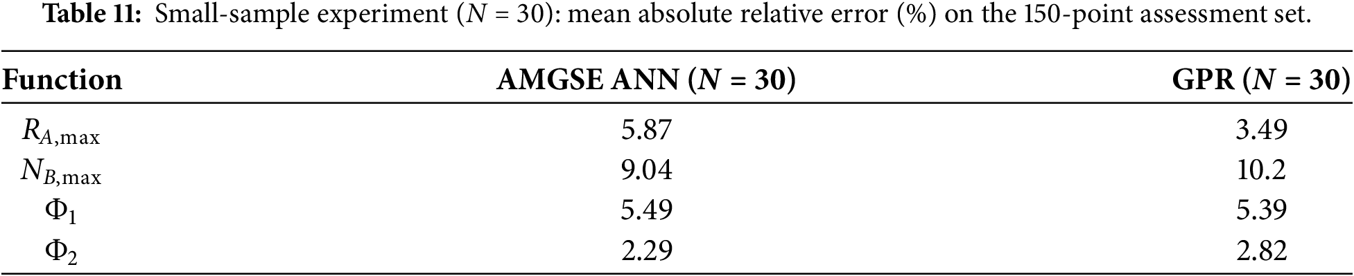
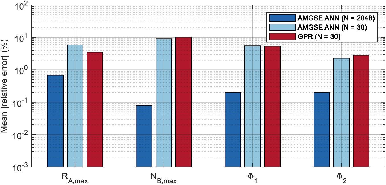
Figure 14: Behavior in the small-sample regime–mean absolute relative error (%) of the AMGSE ANN at N = 2048 and N = 30, and of GPR at N = 30 (logarithmic scale).
4.7.1 How Much of the Inherited Design Was Necessary
Whether the design points should instead be selected by an optimizer is a question that presupposes that the inherited fixed design may be larger than necessary. That premise was tested directly. Surrogates were rebuilt on random subsets of the existing 2048-point dataset of sizes N = 30, 60, 100, 200, 400, 800, 1600 and 2048, with three independent subsets per level (necessarily a single set at N = 2048), and evaluated on the same 150-point assessment set; no additional exact-model evaluation was required. Fig. 15 shows the resulting learning curves. For Φ1 the error falls from 6.92% at N = 30 to 0.368% at N = 400 and 0.220% at N = 1600, and is statistically indistinguishable between N = 1600 and N = 2048. For RA,max the error is still decreasing at the full design size (0.891% at N = 400, 0.826% at N = 800, 0.672% at N = 1600 and 0.599% at N = 2048). Diminishing returns therefore set in around N = 400, but no plateau is reached: on the evidence of these curves, the inherited design was not demonstrably redundant for the two responses examined, and for one of them it was, if anything, not yet saturated. We note that the adaptive-complexity module is active for the three smallest levels, so the left-hand portion of each curve reflects the combined effect of sample size and of that module. The subset sizes, the number of repetitions per level, the seed-generation scheme and the tabulated errors behind Fig. 15 are reported in Supplementary Section S12.
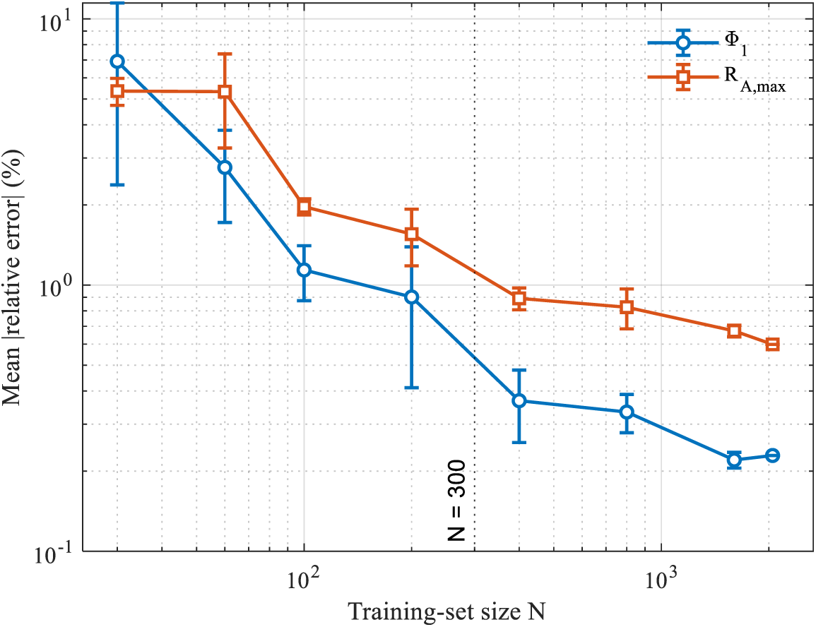
Figure 15: Learning curves of AMGSE (micro level) as a function of training-set size, evaluated on the 150-point independent assessment set. Markers show the mean over three random subsets (a single set at N = 2048); error bars show one standard deviation. Both axes are logarithmic.
4.7.2 Optimizer-Guided Selection of Design Points at a Matched Budget
We next compared design-of-experiments strategies at a matched budget of 160 design points. Three settings were evaluated: a random subset of the existing dataset; a pool-based adaptive selection in which a Gaussian-process model with an anisotropic Matern kernel is refitted after each batch and the ten points of maximum predictive standard deviation are added, starting from a 60-point space-filling design; and the full 2048-point design as an upper reference. Candidate locations were drawn from the existing dataset rather than from the continuous design domain, so the experiment consumes no additional exact-model evaluation and does not depend on an infill implementation of our own; this restriction is stated explicitly because it bounds what the result can support. Table 12 reports the outcome over three seeds. The full-design column of Table 12 is a single reference run of this experiment and is therefore not identical to the ten-run campaign mean discussed in Section 4.3.2.

At a matched budget, the adaptive selection was indistinguishable from random subsampling on both responses, and both were two to five times less accurate than the full design. This outcome is consistent with the nature of the criterion used: a pure maximum-variance rule is an exploration criterion, and on a pool that is already space-filling, it essentially reproduces a space-filling design. The benefits of adaptive sampling are concentrated in goal-oriented settings–expected improvement for optimization, or expected-feasibility refinement near constraint boundaries–which pursue a different objective from the global accuracy required of a surrogate embedded in a population-based evolutionary algorithm. Goal-oriented acquisition functions were not tested here and remain an open question, stated as such in Section 4.8. Fig. 16 summarizes the comparison.
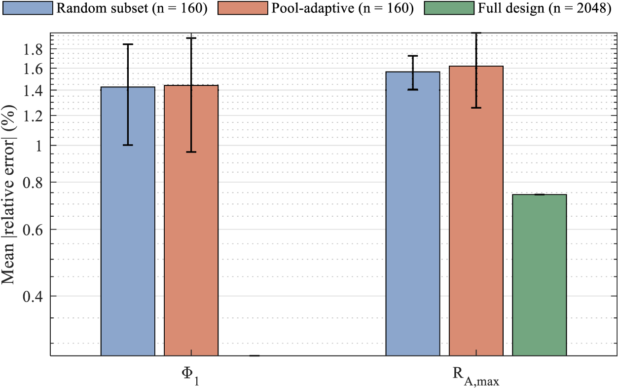
Figure 16: Design-of-experiments strategies at a matched budget of 160 design points, against the full 2048-point design. Bars show the mean over three seeds; error bars show one standard deviation; the vertical axis is logarithmic.
4.7.3 Positioning Relative to Sequential Adaptive-Sampling Methods
Sections 4.7.1 and 4.7.2 address the empirical question. The conceptual distinction is summarized in Table 13. The two paradigms address different bottlenecks: AMGSE extracts the most reliable surrogate from the data already obtained, whereas sequential adaptive sampling reduces the number of expensive evaluations required to obtain data. In the terminology of the data-driven optimization literature, the present setting is an offline one [39], and the framework is compatible with, rather than an alternative to, the online setting.
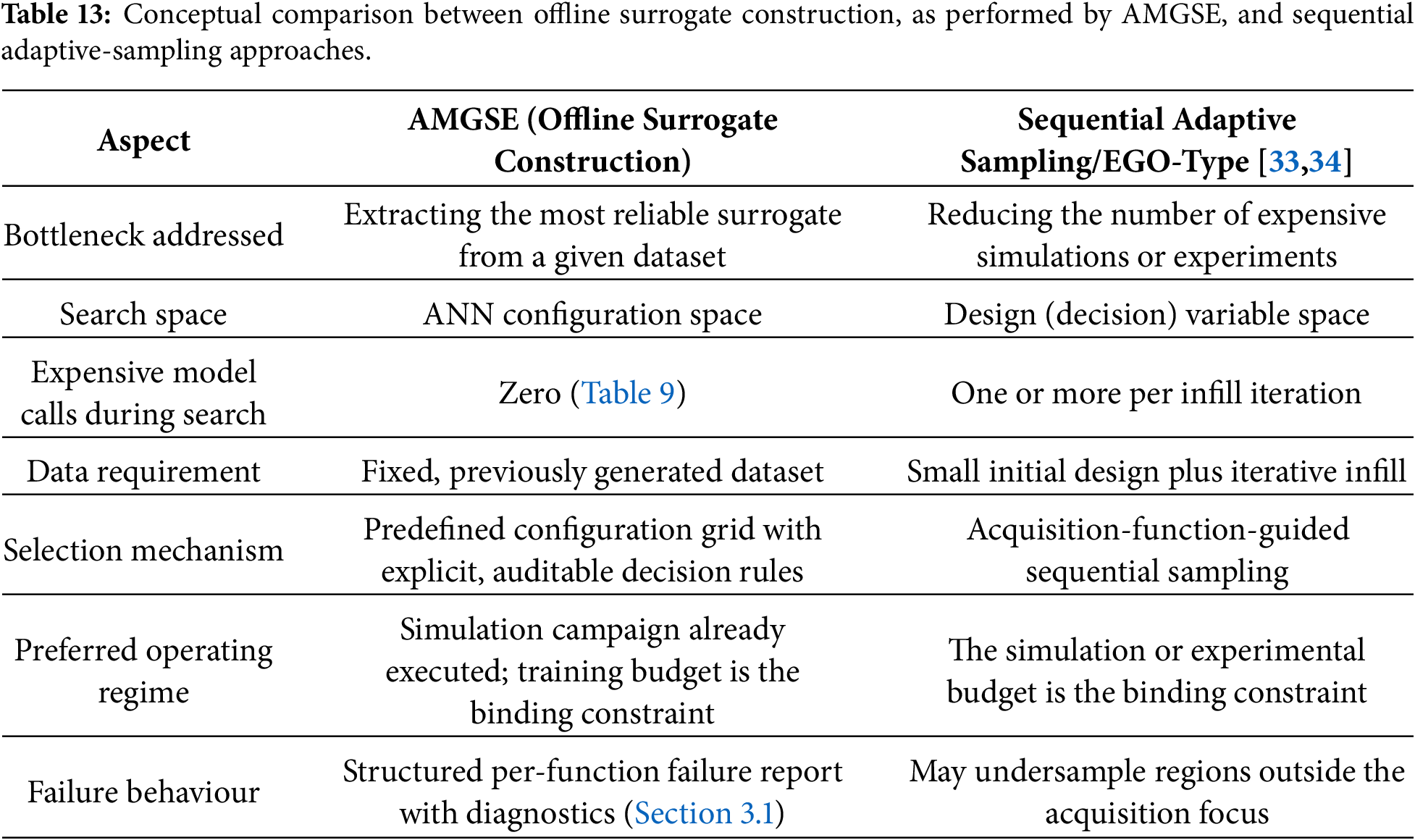
Avenues of improvement. Six concrete directions in which the framework could be extended are identified. First, an outer adaptive-sampling loop with AMGSE as the inner surrogate builder; when the conditional ensemble branch activates, the ensemble-disagreement indicator of Phase 5 supplies a natural acquisition signal, and in the single-model regime, the restart-to-restart prediction spread can serve the same role. Second, goal-oriented acquisition–expected improvement, or expected-feasibility refinement near the constraint boundaries c1 and c2—which Section 4.7.2 did not test. Third, a hybrid configuration grid combined with model-based search over continuous hyperparameters, which would matter once learning rates or regularization strengths are included in the search space. Fourth, multi-fidelity selection of the starting tier. Fifth, a hybrid surrogate-family rule exploiting the accuracy-vs-inference-speed trade-off documented in Section 4.3.3. Sixth, re-assessment of the conditional ensemble rule under noisy multi-physics data, the regime for which it was designed. We state without reservation that optimizer-selected sampling is the single most valuable extension of the present framework.
The evidence presented in this study is subject to the following limitations. First, the engineering validation is confined to a single mechanism-design problem with three design variables, two objectives, and two constraints; although the comparison protocol is rigorous (ten independent runs, statistical testing, independent assessment data, and exact-model re-evaluation of every Pareto candidate), claims of generality beyond this problem class remain to be established. Second, the training budget of the multi-restart grid search grows linearly with the number of configurations and restarts; for problems in which a single ANN training is itself expensive, the medium and large scales may become impractical. Third, the case-study data are deterministic and essentially noise-free, a regime in which the conditional ensemble rule systematically favors the best single model, and in which the ablation study (Section 4.5) found that neither multi-restart training nor forced ensembling provided a measurable accuracy benefit over a single-restart grid-search baseline on the independent assessment set; the benefits of both mechanisms under noisy, multi-physics data, where model-to-model variability is expected to be larger, remain to be quantified. Fourth, AMGSE does not perform active data acquisition; when the number of affordable simulations or experiments is the binding constraint, sequential adaptive-sampling methods are more appropriate (Section 4.7). Fifth, the default decision parameters (complexity scaling 0.7 with a 300-sample threshold; 30% ensemble gap; R = 8 restarts) are heuristics; the ablation study bounds the influence of the restart and gap parameters, but a full sensitivity sweep across problem classes is left for future work. Finally, the implementation is bound to the MATLAB neural-network toolchain; porting the decision rules to other ecosystems is straightforward in principle but has not been demonstrated. Several further limitations are recorded here. The escalation mechanism carries a worst-case overhead: because the four levels are search spaces of increasing cardinality rather than a strictly nested ladder, a response that had to climb every level would consume the sum of the level costs, about 1.8 times the cost of committing directly to the largest level; Section 4.9 provides a measured instance of cumulative escalation through the medium level. The conditional ensemble branch is exercised only sparsely by the present evidence: it is rejected by the gap rule for all four case-study responses and is accepted in only one of the benchmark configurations of Section 4.9, so the practical value demonstrated here lies in the rule-based rejection of ensembling rather than in ensemble construction itself. In addition, the default decision parameters remain heuristics tied to the dimensionality of the present problem: the sample-count trigger of 300 was calibrated on a three-variable response and does not fire at N = 500 in six or eight dimensions, where the sample density per input dimension is far lower; replacing the absolute count by a dimension-aware criterion is identified as future work. The pool-based sampling analysis in Section 4.7.2 used only a pure-exploration acquisition criterion, so no conclusion is drawn about goal-oriented acquisition functions. A further limitation concerns the data-profiling stage, which caps training targets that lie beyond three interquartile ranges from the quartiles. Because the case-study data are deterministic outputs of an exact model rather than noisy measurements, this operation is a winsorization of physically valid response tails and not a correction of erroneous records, and it is reported as such. It modified 133 of the 8192 scalar training targets, concentrated in 77 of the 2048 design points (3.8%), predominantly in the upper tail of the two constraint responses (Supplementary Section S1). Its effect on the optimization can be bounded exactly, because the winsorization thresholds lie far inside the infeasible region: 4947.9 N for RA,max against an allowable 3500 N, and 1451.4 N for NB,max against an allowable 750 N. The 76 designs affected through one of the two constraint responses are therefore infeasible by construction; the single remaining design, affected only through Φ1, was checked directly and also violates both constraints, so a point-by-point audit confirms that all 77 are infeasible, the smallest violation of RA,max being 33% above the allowable value. None could have appeared on a feasible Pareto front, whether or not the rule had been applied. Moreover, the rule reduces large values, so an affected design appears less constrained rather than more, which enlarges rather than contracts the region the optimizer explores; the resulting failure mode is a false-feasible candidate rather than the exclusion of a genuinely feasible trade-off. Mandatory exact-model re-verification is designed to detect exactly that failure mode, and in the present optimization, it identified one infeasible candidate among the 152, although that individual error cannot be attributed specifically to the winsorization. Winsorizing physically valid tails nevertheless remains a preprocessing choice better suited to noisy measurements than to deterministic simulation outputs, and it is not recommended as a default for the latter.
4.9 Generality Check and Behavior of the Escalation Rule on Analytic Benchmarks
Branin, Hartmann-6 and Borehole are adopted here as the natural next step for assessing generality. This section serves a second purpose that the slider-crank case study could not: because all four responses there were accepted at the micro level, the escalation rule of Section 3.1 was never exercised. On these benchmarks, it is. For each benchmark, three mutually independent Latin-hypercube sets were generated with the analytic function: a 500-point training set, a 100-point acceptance set used solely for the pass/fail decision between search levels, and a 150-point assessment set used solely for reporting. This separation also removes the ambiguity identified in Section 3.1, where a single set would otherwise serve both roles. Accuracy is reported as normalized root-mean-square error, NRMSE = RMSE/SD(Y) × 100%, rather than as a relative error, because Hartmann-6 takes values arbitrarily close to zero over its domain and a relative-error metric is not defined there. The acceptance tolerance was fixed a priori at ε = 1% NRMSE.
Three regimes emerge, and dimensionality is not what separates them. Branin, a smooth two-variable response, is fitted with essentially the same accuracy by both surrogate families. Borehole, despite having eight inputs, is also fitted essentially exactly, and the AMGSE-selected ANN is there slightly more accurate than a Gaussian process whose kernel family, basis function and hyperparameters were selected automatically by cross-validation. Hartmann-6, with six inputs but four sharp Gaussian basins, defeats both families at N = 500: the AMGSE ANN reaches 44.6% NRMSE and the tuned Gaussian process 38.2%, a ratio of 1.17. The binding constraint is therefore the multimodality of the response relative to the sample density, not the input dimension or the ANN family as such. That ordering is not a surprise, and reproducing it is the point of the check: the three responses are standard, well-characterized benchmarks (Supplementary Section S13), Borehole a smooth eight-variable function dominated by a few of its inputs, Hartmann-6 a six-variable function with four sharp Gaussian basins. A decision rule that could not separate a nominally higher-dimensional but well-behaved response from a lower-dimensional multimodal one would have little diagnostic value; the agreement between the accept and decline decisions and the established character of these functions is therefore evidence that the acceptance test measures what it is intended to measure, rather than a claim that input dimensionality is immaterial in general.
Table 14 records the behavior of the decision rule itself. On the two responses it can model, the framework stops after four configurations and 32 trainings. On Hartmann-6, it climbs through micro, small, and medium, fails the tolerance at each, and terminates with the structured diagnostic of Section 3.1, reporting insufficient training data and strong nonlinearity relative to the available sample as the likely causes. That diagnosis is independently corroborated: a Gaussian process fitted to the same data with automatic kernel and basis selection reaches 38.2% NRMSE, so the refusal to certify a surrogate reflects a property of the problem at N = 500 rather than a deficiency of the search. The escalation path consumed 256 trainings, that is 0.8 times the 320 required by a direct search of the largest level; because the ladder was capped at the medium level for tractability, this run does not realize the worst case stated in Section 4.8, in which climbing all four levels would consume 576 trainings, about 1.8 times a direct large-level search. The conditional ensemble rule was also exercised in both directions on these benchmarks: at the small level on Hartmann-6, the gap criterion admitted a three-network weighted ensemble, whereas on Borehole it rejected ensembling with a maximum gap far above the 30% threshold. Fig. 17 presents both panels of this analysis. Two caveats are stated explicitly: Hartmann-6 and Borehole were run with a single seed, and the ladder was capped at the medium level for tractability, so Table 14 demonstrates the mechanism rather than a statistical study; and the hyperparameter-optimization baselines in Section 4.3.2 are not reported for the benchmarks. Those runs were attempted on the benchmark files but none completed, for an infrastructure reason rather than a property of the methods: the baseline routines address the data worksheet by index and expect the two-sheet layout of the case-study files, whereas the benchmark data files contain a single worksheet, so the loader fails before any training begins; the same routines executed without incident in the 120 baseline runs of Section 4.3.2; an independently tuned Gaussian process is therefore used as the external comparator in Table 15. This does not bear on the two questions the section addresses–whether the framework transfers to other response classes, and whether the escalation rule behaves as designed–and the baseline comparison itself was carried out on the case study, over ten independent runs with formal significance testing. The analytic definitions of the three benchmarks, the reference optima against which our implementations were verified, and the sampling protocol for the three Latin-hypercube sets are given in Supplementary Section S13.
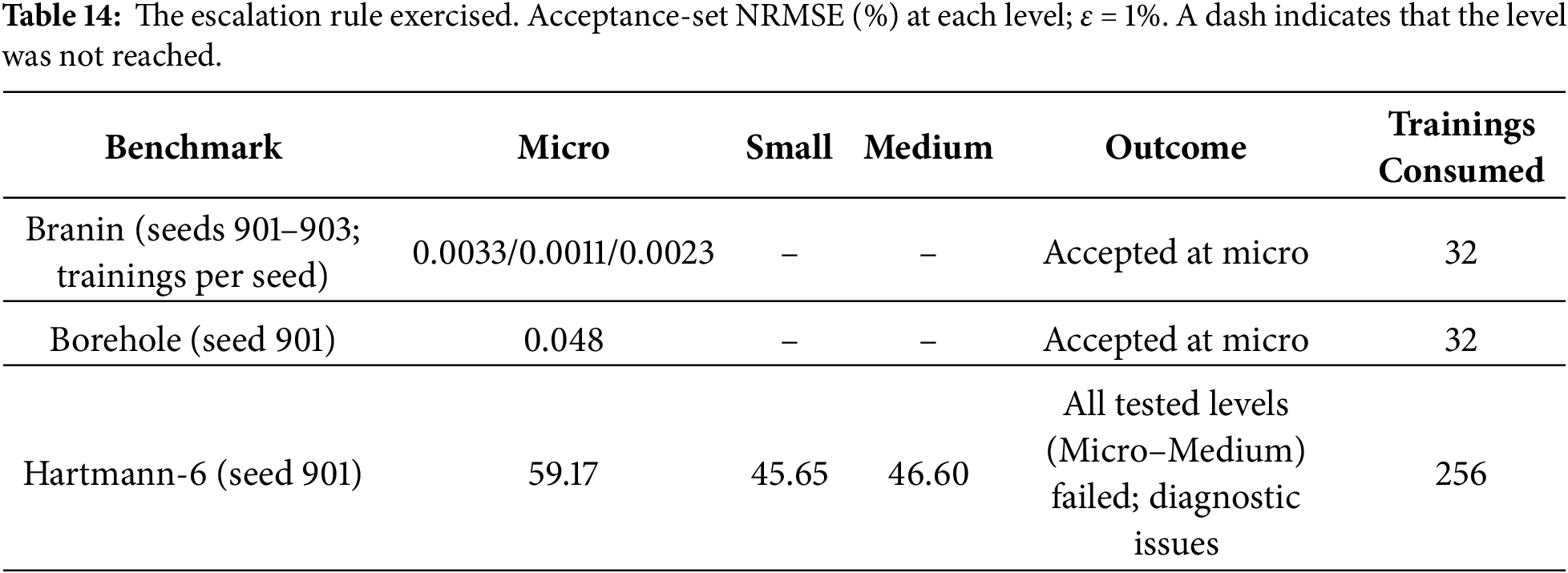
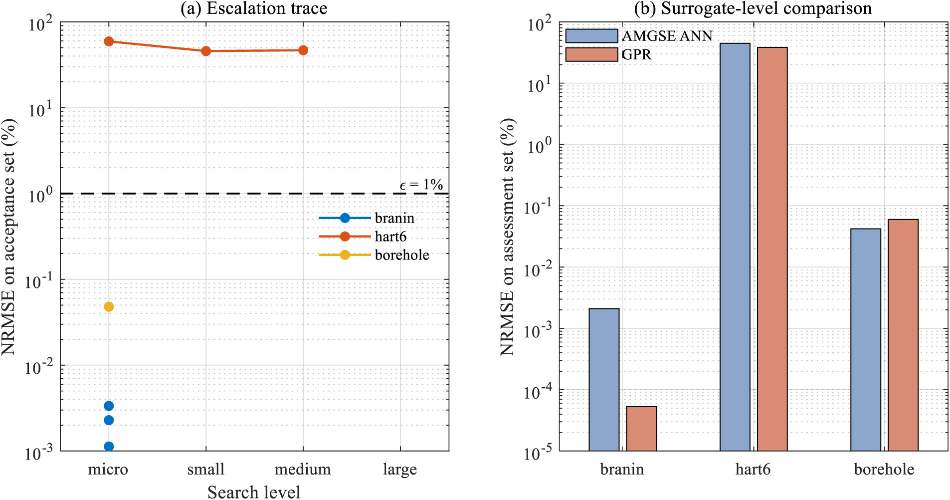
Figure 17: Behavior on the analytic benchmarks. (a) Acceptance-set NRMSE at each search level, with the acceptance tolerance ε = 1% shown as a dashed line; (b) Assessment-set NRMSE of the AMGSE-selected ANN and of a tuned Gaussian process trained on identical data. Both vertical axes are logarithmic.
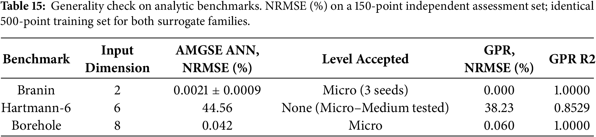
This study introduces the Adaptive Multi-scale Grid Search with Ensemble Integration (AMGSE), an integrated and reproducible framework for optimizing artificial neural network (ANN) surrogate models for computationally intensive engineering optimization problems. By integrating hierarchical multi-scale hyperparameter search, adaptive complexity adjustment, multi-restart training, performance-based ensemble integration, and a conditional ensemble-disagreement characterization (active when the ensemble is selected), AMGSE addresses key challenges in ANN optimization, including time-quality trade-offs, overfitting in small datasets, and prediction reliability.
A systematic comparative evaluation was conducted at two levels. At the hyperparameter-optimization level, under a matched-conditions protocol (matched search spaces and data partitions, with realized computational costs reported separately) repeated over ten independent runs, AMGSE achieved mean prediction errors of 0.11%–0.67% across the four response functions on a 150-point independent assessment set–3.3–10.6 times below Bayesian Optimization, TPE, and Random Search on three of the four functions, and below TPE on the fourth (on which AMGSE was modestly outperformed by Bayesian Optimization and Random Search)–with all Friedman and Holm-corrected Wilcoxon tests significant at p < 0.01. At the surrogate level, Gaussian process regression attained the lowest error on three of the four functions, consistent with its known strength on smooth, low-dimensional responses, while the AMGSE-selected ANN attained the lowest error on the remaining function and retained an advantage in batch-inference speed. An ablation study found that multi-restart training and the conditional ensemble rule contributed little measurable accuracy benefit on this case study relative to a single-restart grid-search baseline, indicating that the systematic grid coverage of the micro-scale search, rather than these two mechanisms individually, is the primary driver of AMGSE’s accuracy advantage; they nonetheless provide a safety margin against poor initializations without an accuracy cost resolvable at the five-run resolution of that study.
Applied to the multi-objective optimization of spring placement and stiffness in slider-crank mechanisms to enhance dynamic performance, the AMGSE–NSGA-III pipeline produced a larger, better-performing verified Pareto set than the previously reported CDOS-PSI solutions. Using prior evaluation data, the framework trained accurate surrogate models that enabled NSGA-III to identify 152 surrogate-nondominated candidates, of which 151 were verified as feasible against the exact model and 150 were mutually non-dominated under exact objectives (146 distinct objective vectors)–outperforming the previous grid-based CDOS-PSI method’s 19 solutions in both quantity and quality. The surrogate models achieved RMSPE between 0.59% and 3.11% on the 150-point independent assessment set, facilitating rapid design-space exploration; at the inference level, the ANN surrogate evaluates candidate batches two to three orders of magnitude faster than GPR and RBF (Supplementary Section S10.1), a practical advantage inside the evolutionary optimization loop.
Within the scope delineated in Section 4.8, the results underscore AMGSE’s potential for surrogate modeling in complex dynamical systems, offering improved predictive accuracy, ensemble-based disagreement estimation (when conditional ensembling is active), and efficient integration with advanced optimization algorithms. Future work will explore extensions to many-objective problems, the incorporation of active learning for adaptive data collection, and applications in multiphysics domains with inherent noise and uncertainty. Two additions of the present revision bear directly on the scope of these claims. A flat search over a fivefold larger configuration space reduced the assessment error of Φ1 by about ten percent, an improvement that lies at the edge of the run-to-run band of the hierarchical stop and that one of ten micro-scale runs matched unaided; the hierarchy is therefore justified as a resource-allocation protocol rather than as a route to higher accuracy. On analytic benchmarks spanning two, six, and eight input dimensions, the framework transfers without modification to the two responses that a 500-point design can support, and on the third, it declines to certify a surrogate and reports why–a refusal independently corroborated by a tuned Gaussian process on the same data. We regard this explicit delineation of the operating envelope, together with the negative findings retained in Sections 4.5, 4.3.3 and 4.7, as part of the contribution rather than a qualification of it. More broadly, the elements that make the pipeline auditable—a stated training-time budget, a capacity rule keyed to sample size, restart-and-select, a gap-thresholded ensemble veto, and an external acceptance test that every surrogate must pass before downstream use–depend on nothing specific to mechanism design. They require a dataset already generated from an expensive model, a stated training-time budget, and a prespecified acceptance tolerance. Surrogate-assisted design problems with this structure arise in computational mechanics, thermo-fluid and multiphysics analysis, structural and materials optimization, and process design; whether the protocol behaves in those settings as it does here–certifying when the data support a surrogate and refusing when they do not—is not established by the present evidence, and is the limitation recorded in Section 4.8.
Acknowledgement: Many thanks are due to the Engineering Mathematics Research Group (EMRG) of the Industrial University of Ho Chi Minh City for the motivation that helped us complete this research.
Funding Statement: This research is supported by Industrial University of Ho Chi Minh City (IUH) under grant number 65/HD-DHCN, dated 11/12/2025.
Author Contributions: The authors confirm contribution to the paper as follows: study conception and design: Hoang Minh Dang, Van Binh Phung; data collection: Hoang Minh Dang; analysis and interpretation of results: Hoang Minh Dang, Van Binh Phung; draft manuscript preparation: Hoang Minh Dang, Van Binh Phung, Van Thanh Tien Nguyen. All authors reviewed and approved the final version of the manuscript.
Availability of Data and Materials: All experiments were performed in MATLAB (Student version) on an Intel Core i7 vPro processor with 64 GB of memory; the exact-model verification computations were performed in Maple. Random seeds are fixed as reported (HPO campaign seeds 101–110; ablation seeds 501–505; small-sample seeds 2026–2035; flat-search arm seed 601; design-of-experiments seeds 801–803; analytic-benchmark seeds 901–903). The 150-point external evaluation dataset and the exact-model verification data supporting the findings of this study are available from the corresponding author upon reasonable request. The MATLAB implementation of the AMGSE framework is part of an ongoing proprietary research infrastructure and is not publicly available at this time.
Ethics Approval: Not applicable. This study did not involve human participants or animals.
Conflicts of Interest: The authors declare no conflicts of interest.
Supplementary Materials: The supplementary material is available online at https://www.techscience.com/doi/10.32604/cmes.2026.086495/s1.
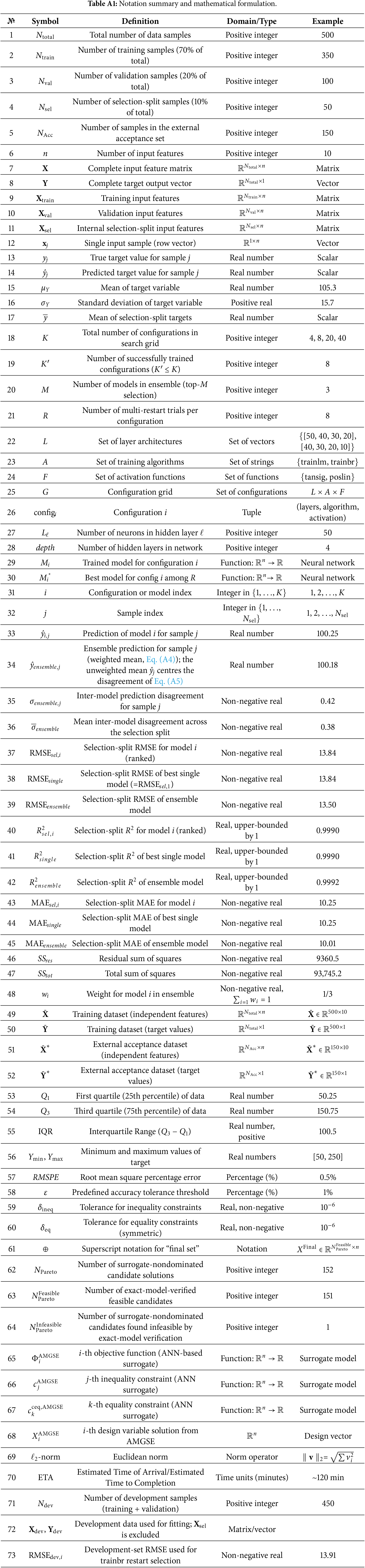
Appendix B Detailed Methodology Descriptions and Mathematical Formulations
For reasons of length, the detailed phase-by-phase methodology descriptions and mathematical formulations are provided in the Supplementary Material (Sections S1–S6), which also includes the distribution plots of the ten-run comparison campaign (Fig. S1). The main-text description of the six phases is given in Section 2.
Appendix C PSEUDO-CODE

References
1. Du X, Xu H, Zhu F. Understanding the effect of hyperparameter optimization on machine learning models for structure design problems. Comput Aided Des. 2021;135(5):103013. doi:10.1016/j.cad.2021.103013. [Google Scholar] [CrossRef]
2. Ghafariasl P, Mahmoudan A, Mohammadi M, Nazarparvar A, Hoseinzadeh S, Fathali M, et al. Neural network-based surrogate modeling and optimization of a multigeneration system. Appl Energy. 2024;364(12):123130. doi:10.1016/j.apenergy.2024.123130. [Google Scholar] [CrossRef]
3. Khatouri H, Benamara T, Breitkopf P, Demange J. Metamodeling techniques for CPU-intensive simulation-based design optimization: a survey. Adv Model Simul Eng Sci. 2022;9(1):1. doi:10.1186/s40323-022-00214-y. [Google Scholar] [CrossRef]
4. Abdolrasol MGM, Hussain SMS, Ustun TS, Sarker MR, Hannan MA, Mohamed R, et al. Artificial neural networks based optimization techniques: a review. Electronics. 2021;10(21):2689. doi:10.3390/electronics10212689. [Google Scholar] [CrossRef]
5. Soori M, Karimi F, Jough G. Artificial intelligent in optimization of steel moment frame structures: a review. Int J Struct Constr Eng. 2024;18(3):1–19. [Google Scholar]
6. Sun G, Wang S. A review of the artificial neural network surrogate modeling in aerodynamic design. Proc Inst Mech Eng Part G J Aerosp Eng. 2019;233(16):5863–72. doi:10.1177/0954410019864485. [Google Scholar] [CrossRef]
7. Han SS, Kim HK. Artificial neural network-based sequential approximate optimization of metal sheet architecture and forming process. J Comput Des Eng. 2024;11(3):265–79. doi:10.1093/jcde/qwae049. [Google Scholar] [CrossRef]
8. Amakor AC, Berkemeier MB, Wohlleben M, Sextro W, Peitz S. Surrogate-assisted multi-objective design of complex multibody systems. In: Proceedings of the 34th International Conference on Artificial Neural Networks and Machine Learning, ICANN 2025; 2025 Sep 9–12; Kaunas, Lithuania. p. 251–62. [Google Scholar]
9. Tejero F, MacManus D, Heidebrecht A, Sheaf C. Artificial neural network for preliminary design and optimisation of civil aero-engine nacelles. Aeronaut J. 2024;128(1328):2261–80. doi:10.1017/aer.2024.38. [Google Scholar] [CrossRef]
10. Massoudi S, Picard C, Schiffmann J. Robust design using multiobjective optimisation and artificial neural networks with application to a heat pump radial compressor. Des Sci. 2022;8:e1. doi:10.1017/dsj.2021.25. [Google Scholar] [CrossRef]
11. Persia JT, Sung MK, Lee S, Burns DE. Neural network-based surrogate model in postprocessing of topology optimized structures. Neural Comput Appl. 2025;37(15):8845–67. doi:10.1007/s00521-025-11039-2. [Google Scholar] [CrossRef]
12. Nikzad MH, Heidari-Rarani M, Mirkhalaf M. A novel Taguchi-based approach for optimizing neural network architectures: application to elastic short fiber composites. Compos Sci Technol. 2025;259:110951. doi:10.1016/j.compscitech.2024.110951. [Google Scholar] [CrossRef]
13. Lee S, Kang N. Vehicle suspension recommendation system: multi-fidelity neural network-based mechanism design optimization. Struct Multidiscip Optim. 2025;68(3):44. doi:10.1007/s00158-024-03957-x. [Google Scholar] [CrossRef]
14. Morales-Hernández A, Van Nieuwenhuyse I, Rojas Gonzalez S. A survey on multi-objective hyperparameter optimization algorithms for machine learning. Artif Intell Rev. 2023;56(8):8043–93. doi:10.1007/s10462-022-10359-2. [Google Scholar] [CrossRef]
15. Adekunle AA, Fofana I, Picher P, Rodriguez-Celis EM, Arroyo-Fernandez OH, Zemouri R. Optimizing deep learning predictive models: a comprehensive review of RNN and its variant architectures. Appl Soft Comput. 2025;185(3):114015. doi:10.1016/j.asoc.2025.114015. [Google Scholar] [CrossRef]
16. Bergstra J, Bengio Y. Random search for hyper-parameter optimization. J Mach Learn Res. 2012;13:281–305. [Google Scholar]
17. Snoek J, Larochelle H, Adams RP. Practical Bayesian optimization of machine learning algorithms. Adv Neural Inf Process Syst. 2012;25:2960–8. doi: 10.48550/arxiv.1206.2944. [Google Scholar] [CrossRef]
18. Bergstra J, Bardenet R, Bengio Y, Kégl B. Algorithms for hyper-parameter optimization. Adv Neural Inf Process Syst. 2011;24:2546–54. [Google Scholar]
19. Young SR, Rose DC, Karnowski TP, Lim SH, Patton RM. Optimizing deep learning hyper-parameters through an evolutionary algorithm. In: Proceedings of the Workshop on Machine Learning in High-Performance Computing Environments; 2015 Nov 15; Austin, TX, USA. [Google Scholar]
20. López-González N, Rodríguez E, Greiner D. A multi-objective evolutionary computation approach for improving neural network-based surrogate models in structural engineering. Algorithms. 2025;18(12):754. doi:10.3390/a18120754. [Google Scholar] [CrossRef]
21. Wang Y, Han X, Chang CY, Zha D, Braga-Neto U, Hu X. Auto-PINN: understanding and optimizing physics-informed neural architecture. arXiv:2205.13748. 2022. [Google Scholar]
22. Zhou ZH. Ensemble methods: foundations and algorithms. Boca Raton, FL, USA: CRC Press; 2012. [Google Scholar]
23. Goel T, Haftka RT, Shyy W, Queipo NV. Ensemble of surrogates. Struct Multidiscip Optim. 2007;33(3):199–216. doi:10.1007/s00158-006-0051-9. [Google Scholar] [CrossRef]
24. Acar E, Rais-Rohani M. Ensemble of metamodels with optimized weight factors. Struct Multidiscip Optim. 2009;37(3):279–94. doi:10.1007/s00158-008-0230-y. [Google Scholar] [CrossRef]
25. Takenaga S, Ozaki Y, Onishi M. Parameter-free dynamic fidelity selection for automated machine learning. Appl Soft Comput. 2025;171:112750. doi:10.1016/j.asoc.2025.112750. [Google Scholar] [CrossRef]
26. Elsken T, Metzen JH, Hutter F. Neural architecture search: a survey. J Mach Learn Res. 2019;20(55):1–21. doi:10.1007/978-3-030-05318-5_3. [Google Scholar] [CrossRef]
27. Thornton C, Hutter F, Hoos HH, Leyton-Brown K. Auto-WEKA: combined selection and hyperparameter optimization of classification algorithms. In: Proceedings of the 19th ACM SIGKDD International Conference on Knowledge Discovery and Data Mining; 2013 Aug 11–14; Chicago, IL, USA. p. 847–55. [Google Scholar]
28. Feurer M, Klein A, Eggensperger K, Springenberg JT, Blum M, Hutter F. Auto-sklearn: efficient and robust automated machine learning. In: Automated machine learning: methods, systems, challenges. Cham, Switzerland: Springer; 2019. p. 113–34. [Google Scholar]
29. Sun L. Automated neural network architecture design and hyperparameter adjustment integrating distribution-based optimization strategy. Appl Comput Eng. 2025;147(1):181–6. doi:10.54254/2755-2721/2025.22721. [Google Scholar] [CrossRef]
30. Vincent AM, Jidesh P. An improved hyperparameter optimization framework for AutoML systems using evolutionary algorithms. Sci Rep. 2023;13(1):4737. doi:10.1038/s41598-023-32027-3. [Google Scholar] [CrossRef]
31. Li Q, Kamaruddin N, Zhang J, Peng C, Sui Ki Khoo A. A novel method of Bayesian genetic optimization on automated hyperparameter tuning. Sci Rep. 2025;15(1):43181. doi:10.1038/s41598-025-29383-7. [Google Scholar] [CrossRef]
32. Dang HM, Phung VB, Nguyen VTT. Multi-objective optimizing spring placement and stiffness in slider-crank mechanisms for enhanced dynamic parameters. PLoS One. 2025;20(9):e0331341. doi:10.1371/journal.pone.0331341. [Google Scholar] [CrossRef]
33. Jones DR, Schonlau M, Welch WJ. Efficient global optimization of expensive black-box functions. J Glob Optim. 1998;13(4):455–92. doi:10.1023/A:1008306431147. [Google Scholar] [CrossRef]
34. Liu Z, Huang H, Xu X, Xiong M, Li Q. An efficient global optimization algorithm combining revised expectation improvement criteria and Kriging. Eng Optim. 2024;56(4):608–24. doi:10.1080/0305215X.2023.2170367. [Google Scholar] [CrossRef]
35. Jain H, Deb K. An evolutionary many-objective optimization algorithm using reference-point based nondominated sorting approach, part II: handling constraints and extending to an adaptive approach. IEEE Trans Evol Comput. 2014;18(4):602–22. doi:10.1109/TEVC.2013.2281534. [Google Scholar] [CrossRef]
36. Deb K, Jain H. An evolutionary many-objective optimization algorithm using reference-point-based nondominated sorting approach, part I: solving problems with box constraints. IEEE Trans Evol Comput. 2014;18(4):577–601. doi:10.1109/TEVC.2013.2281535. [Google Scholar] [CrossRef]
37. Deb K, Pratap A, Agarwal S, Meyarivan T. A fast and elitist multiobjective genetic algorithm: NSGA-II. IEEE Trans Evol Comput. 2002;6(2):182–97. doi:10.1109/4235.996017. [Google Scholar] [CrossRef]
38. Das I, Dennis JE. Normal-boundary intersection: a new method for generating the Pareto surface in nonlinear multicriteria optimization problems. SIAM J Optim. 1998;8(3):631–57. doi:10.1137/s1052623496307510. [Google Scholar] [CrossRef]
39. Wang H, Jin Y, Sun C, Doherty J. Offline data-driven evolutionary optimization using selective surrogate ensembles. IEEE Trans Evol Comput. 2019;23(2):203–16. doi:10.1109/tevc.2018.2834881. [Google Scholar] [CrossRef]
Cite This Article
 Copyright © 2026 The Author(s). Published by Tech Science Press.
This work is licensed under a Creative Commons Attribution 4.0 International License , which permits unrestricted use, distribution, and reproduction in any medium, provided the original work is properly cited.
 Downloads
 Citation Tools
