A Novel Multiscale Approach for Modelling Fracture Response of Heterogeneous Materials

1  Introduction

At their lower levels, modern engineering materials often exhibit a significant material heterogeneity. This heterogeneity manifests itself in the form of different microconstituents (material phases) with arbitrary shape, volume fraction, spatial distribution and mechanical properties [1]. Therefore, the overall mechanical behaviour of the material is the result of the mutual interaction and contribution of each of its microconstituents. This becomes particularly important when numerical modelling of damage and fracture is considered.

In the field of numerical modelling of damage and fracture in heterogeneous materials, multiscale analysis [2] is a valuable tool since it allows for the coupling of the microstructural stress state with the macroscopic calculation. Concurrent multiscale methods [3–5] (a class of multiscale methods) achieve this coupling by homogenising (averaging) the values at the microlevel, which are then used for the analysis at each macroscopic point. This essentially ensures a full incorporation of the material heterogeneity into the numerical model, thus providing a more accurate modelling in contrast to the classical phenomenological approach [6]. Alongside higher accuracy, concurrent multiscale analysis also introduces the need for significant computational resources. This is because homogenised values at the macroscopic point are a direct result of the boundary value analysis of the microstructure, which is defined through the representative volume element, i.e., RVE [7–10]. When the boundary value problem at both micro and macrolevel is tackled using finite element method (FEM) [11,12], fast Fourier transform (FFT) [13], advanced mesh-superposition formulations like the s-version of FEM [14] or when a mixed approach is used [15,16], the total computation cost will reach unacceptable levels. Calculation of the RVE boundary value problem at each macroscopic point via direct numerical simulation, i.e., DNS (either through FEM or FFT), is the main reason for the high computational cost, which only increases when damage enters the equation. Moreover, the incorporation of damage analysis into a concurrent multiscale approach requires consideration of issues related to mesh dependence at the macrolevel [1,17], calculation of the macroscopic value of damage [18,19] and RVE representativeness during strain softening [20,21]. In the recent decade, data-driven multiscale methods have become particularly attractive. As the exponential rise in computational resources allows for storage and analysis of large amounts of raw data, the cost of DNS analysis of the RVE boundary value problem can be dramatically decreased. For instance, neural networks (NNs) have experienced great success in multiscale modelling of heterogeneous materials. With the appropriate architecture and sufficient amount of data, NNs are able to model mechanical response of heterogeneous materials with porosity [22], hyperelastic heterogeneous materials [23,24], elastoplastic [25,26] and even granular like materials [27]. However, their applicability in multiscale modelling of damage and fracture of heterogeneous materials is still quite challenging [28,29]. Highly non-linear and history-dependent phenomenon such as damage requires careful consideration of the type of NN to be used, which, in addition to the need for a large amount of raw data, adds another layer of complexity. In contrast to NNs, reduced-order models (ROMs) target the problem of low computational efficiency of the concurrent multiscale simulation by reducing the number of degrees of freedom (DOF) of the RVE boundary value problem. Over the last decade, many ROMs have been proposed, most notably transformation field analysis [30], non-uniform transformation field analysis [31] and proper orthogonal decomposition [32]. In recent years, a class of data-driven cluster-based ROMs has emerged [33,34]. Different from the mentioned ROMs, cluster-based ROMs are based on discretisation of the RVE into large subdomains called clusters, and the utilisation of a Lippmann-Schwinger equation [35]. A cluster-based ROM called self-consistent clustering analysis (SCA), formulated by Liu et al. [33], represents a pioneering work in this category. Shortly after it was introduced, SCA quickly attracted lots of attention and a large number of contributions [17,36–43] have shown its capabilities in solving the RVE boundary value problem in an accurate and computationally efficient way. A particularly important feature of the SCA is its applicability to different types of RVEs [41–43], constitutive laws [33,39], but also problems of small [33,41,42] as well as finite strains [37,38]. Because of the above, SCA is actively being developed in order to simulate damage and fracture of heterogeneous materials [17,40,44–47]. Being first in this category, contribution [17] represents a major milestone in the field of concurrent multiscale modelling of damage in heterogeneous materials. The approach presented in [17] not only met the requirement of computational efficiency, it also introduced a novel three-step homogenization scheme and a non-local formulation at the macroscopic level. However, this procedure has two main drawbacks. Firstly, the calculation of damage in the microstructural domain, which is decomposed into a relatively small number of clusters, cannot be performed without energy regularisation, i.e., subsequent calibration of the damage parameters using DNS. The second drawback follows from the damage formulation itself, which requires that the energy dissipated by plasticity is negligible compared to the energy dissipated during elastic deformation. Following the idea of FEM h-adaptivity, in [48], authors aimed to mitigate the first issue by proposing an adaptive cluster-based ROM in which the number of clusters can be increased during the analysis. The approach aims to improve the clusters resolution in order to achieve a better description of localised microstructural fields such as plasticity or damage, and was utilised in [44,45] for modelling damage in 3D woven composites. However, the process of h-adaptivity in a cluster-based ROM is not physically justified since cluster discretisation is not the product of a direct geometrical decomposition of an RVE; rather, it is the result of grouping of points which exhibit similar mechanical behaviour. Furthermore, the main goal of a cluster-based ROM is to accurately calculate homogenised values of an RVE, not to give a smooth and detailed description of highly localised fields. But most importantly, this approach is not suitable for large concurrent multiscale analysis since the process of reclustering would need to be performed hundreds (if not thousands of times) since each macroscopic point is directly linked to an RVE. Damage analysis of a 3D woven composites was also the subject of the work done by Li et al. [46], while in [47], alongside experimental investigation, numerical modelling of damage in concrete with the help of the SCA and a concrete micromechanical model [49] was presented. Although the results of [46,47] show a good match with the experimental results, both contributions do not represent a fully concurrent multiscale approach since the link between macroscopic and microscopic level is present only at one point. This is also true for the work presented in [40], where experimental and numerical investigation was done on a 3D braided composites, but again, without the presence of a fully concurrent multiscale procedure.

Although ROMs have the ability to significantly improve the computational efficiency at the microlevel, the problem of pathological mesh dependence at the macrolevel must be addressed separately. The aforementioned contribution [17] showed that the presence of a non-local formulation at the macrolevel is not an option but a necessity in preventing physically meaningless results. Over the years, several methods have been proposed to mitigate the problem of mesh dependence, which occurs during strain softening. One such method, called phase-field (PF) fracture formulation [50], represents a well-established non-local continuum damage model. The PF method has proven to be an accurate and robust procedure for solving problems of damage and fracture for both small [50–52] and finite strains configuration [53,54], under static [51,55,56] and dynamic loading [56,57], as well as fatigue-induced fracture [52,58]. Furthermore, the PF method has successfully been implemented to model fracture in various types of materials, including brittle [50,58,59], ductile [53,58], hyperelastic [60] and viscoelastic–viscoplastic materials [61]. To eliminate mesh dependence and ensure objective and physically meaningful results, PF relies on the use of two parameters, i.e., the length-scale parameter and a critical value of energy release rate. The former helps to diffuse (smear) the sharp crack topology over a finite region, while the latter limits the energy dissipation per unit area in the crack region. For a comprehensive review and more details on the PF method itself, see [62].

In this manuscript, a new, fully concurrent two-scale approach for modelling damage and fracture in both brittle and ductile heterogeneous materials is presented. The proposed procedure aims to tackle issues and shortcomings in the field of numerical modelling of damage and fracture in heterogeneous materials by combining some of the best features of both SCA and the PF fracture method. By employing the SCA at the microlevel, the framework ensures fast, accurate and reliable calculation of the RVE boundary value problem. On the other hand, the utilisation of a non-local damage model, such as PF, at the macrolevel enables objectivity and robustness, but also eliminates mesh dependence at the macrolevel. The full decoupling of the damage analysis from the RVE boundary value problem is an important characteristic of the procedure, which sets it apart from other algorithms. This novelty opens up the possibility for a more stable and computationally efficient calculation of damage and fracture in heterogeneous materials. Because of that, the analysis of the macroscopic material degradation does not include any kind of damage analysis at the microlevel. The generated RVE will serve exclusively for obtaining the homogenised (macroscopic) values, primarily the macroscopic stress tensor, material tangent and strain energy density. By upscaling the macroscopic values, the PF fracture algorithm will receive all the necessary input for the determination of the macroscopic material degradation level.

The paper is organised as follows. The first ingredient of the proposed approach, i.e., the SCA, is briefly described in Section 2. Section 3 gives a short overview of the PF method and its implementation into the finite element method (FEM) framework for modelling damage and fracture in both brittle and ductile materials. In Section 4, a new concurrent multiscale procedure is presented and described in detail. Section 5 includes results related to the accuracy and computational efficiency of the developed procedure obtained by means of numerical simulations on different microstructures and geometrical specimens. Influence of the PF fracture parameters, namely the length-scale parameter and the critical value of energy release rate, on the fracture behaviour is the subject of Section 6, while concluding remarks are given in the last section, i.e., Section 7.

2  Reduced-Order Homogenization

2.1 Self-Consistent Clustering Analysis

The self-consistent clustering analysis (SCA) [33] represents a data-driven, reduced-order homogenization method that allows for computationally efficient and accurate calculation of the RVE boundary value problem. This is achieved through two major innovations: (1) the use of data compression algorithm (k-means clustering [63] or self-organizing map [64]) that drastically reduces the number of degrees of freedom (DOF) by decomposing the RVE into large subdomain (clusters), and (2) a cluster-based numerical procedure for the RVE boundary value problem calculation—which is applicable to any constitutive law of each material phase, without the need for additional calculation. The whole SCA procedure can be broken down into two steps—offline and online. Conveniently, the first innovation is performed in the offline step, while the online step is related to the second innovation. In what follows, a brief description of the SCA and its two steps is given.

2.2 Offline and Online Step

The offline step represents a first stage of the SCA, which needs to be performed only once, but the quality of its execution will greatly impact speed as well as the accuracy of the final solution. It tackles the problem of low computational efficiency at the microlevel, by discretising the RVE in question into a finite number of large subdomains, i.e., material clusters—Fig. 1.

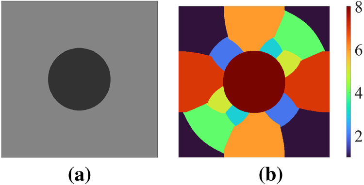
Figure 1: Microstructure decomposition into an appropriate number of material clusters: (a) 2D unit cell geometry; (b) Discretisation with 8 material clusters.

Each material phase in the RVE is represented by a minimum of one material cluster, and the distribution of any arbitrary local variable η inside the cluster is constant [33]. Although this leads to discontinuous distribution of any local variable η, its averaged (homogenised) value η¯ which is given by

η¯=∑I=1kηIcIΩ,(1)

can be calculated with high accuracy using a relatively small number of material clusters. In the averaging equation above, k stands for the total number of material clusters, cI defines the volume fraction of the I-th material cluster in the RVE defined by the volume Ω.

Before the actual decomposition into material clusters, the microstructure first needs to be discretised by an appropriate number of finite elements. This discretisation is necessary since the clustering analysis by itself always involves grouping of points that have similar behaviour into one cluster. The points in this case are finite elements, and the similarity between them is determined by their mechanical behaviour. More precisely, points that exhibit similar mechanical behaviour are placed together into one material cluster using machine learning algorithms such as k-means clustering or self-organising map. This similarity is expressed using strain concentration tensor A, defined as [33]

ε(x)=A(x):ε¯,(2)

where ε¯ denotes the homogenised (macroscopic) value of the small strain tensor, while ε represents the microscopic small strain tensor. Although the number of finite elements (with which the RVE domain is discretised) is arbitrary, it is beneficial to use high resolution as it will allow for an accurate description of both RVE geometry and the microstructural strain field.

The second part of the SCA is called the online step and, in plain terms, represents the calculation of the RVE boundary value problem using the information from the previous (offline) step. The analysis is performed with the help of the incremental form of the Lippmann-Schwinger equation, which is discretised by clusters [33]

ΔεI+∑J=1kDIJ:[ΔσJ−C0:ΔεJ]−Δε0=0,(3)

where Δε defines incremental small strain tensor, Δσ stands for incremental Cauchy stress tensor, C0 is the so-called reference material stiffness tensor, Δε0 represents the incremental far-field small strain tensor while the DIJ denotes the interaction tensor. In the identity above, indices I and J range from 1 to k, and simply determine the current cluster number.

The interaction tensor DIJ, which is given by the double volume integral of the Green’s function G0(x,x′)

DIJ=1cIΩ∫Ω∫ΩχI(x)χJ(x′)G0(x, x′)dx′dx,(4)

is an important ingredient of the online step of the SCA. In essence, it gives the information on how the stress in the J−th cluster is influencing the strain in the I−th cluster. Its value can be determined in numerous ways [39,65]; however, in this study, a fast Fourier transform (FFT) algorithm alongside the Green’s function (defined in the frequency domain) is adopted. In the case of a linearly elastic reference material, the Green’s function is known explicitly and can be expressed in terms of the frequency vector ξ and Lamé parameters of the reference material (λ0 and μ0) as

G^ijkl0(ξ)=14μ0G^ijkl1(ξ)+λ0+μ0μ0(λ0+2μ0)G^ijkl2(ξ),(5)

where G^ijkl1(ξ) and G^ijkl2(ξ) are expressed as

G^ijkl1(ξ)=1ξmξm(δikξjξl+δilξjξk+δjlξiξk+δjkξiξl),(6)

and

G^ijkl2(ξ)=−ξiξjξkξlξmξmξnξn.(7)

In most problems, the incremental stress in the J-th cluster ΔσJ is a nonlinear function of the incremental strain ΔεJ, which means that the system of equations given by Eq. (3) requires an iterative approach in each increment of the analysis. Herein, as is the case in most studies, an implicit type of analysis is adopted. The unknown variables of the system are: incremental strain in each cluster ΔεI and the incremental far field strain Δε0. For the case of macro-strain constraint, the residual of the integral equation in the cluster I is defined as

rI=ΔεI+∑J=1kDIJ:[ΔσJ−C0:ΔεJ]−Δε0=0,(8)

while the remaining part of the residual vector r is equal to

rk+1=∑I=1kcIΔε−Δε¯,→Δε0=Δε¯.(9)

However, the SCA also accepts the macro-stress constraint, where a macroscopic value of Cauchy stress tensor σ¯ is prescribed on the RVE. In that case, only the last part of the residual vector r needs to be modified, i.e.,

rk+1=∑I=1kcIΔσ−Δσ¯.(10)

This ultimately allows the use of the SCA for both displacement as well as force boundary conditions at the macrolevel, providing an additional level of applicability to a broad range of problems.

To maintain self-consistency and ensure a high level of accuracy, the SCA utilises the recalculation of the reference material parameters after each converged increment. Recalculation is done such that new Lamé parameters approximate the homogenised material stiffness in an optimal way, i.e., C0→C¯. This can be utilised using either regression- or projection-based approach [34]. The former represents a more accurate but also more unstable approach when compared with the latter [1]. Although the value of the interaction tensor DIJ changes during the online part of the SCA, the compact form of Eq. (5) means FFT does not need to be performed in each increment. Rather, it is applied once, in the offline part of the SCA.

3  Numerical Modelling of Damage and Fracture

3.1 Phase-Field Method

Generally speaking, phase-field (PF) modelling represents an approach for the description of the behaviour of physical systems that consists of two or more phases that are divided by sharp interfaces. It achieves this by introducing a continuous field variable (order parameter), which differentiates between multiple physical phases within a given system through a smooth transition. When talking about numerical modelling of damage and fracture, such an order parameter describes a gradual evolution from intact to fully broken material, thus serving as a diffuse approximation of a sharp crack discontinuity. Due to its simplicity, robustness, and applicability to a wide range of different materials and different types of fracture, the PF method has earned its reputation as one of the most popular methods for numerical modelling of damage and fracture. The next subsection represents a brief description of the PF fracture formulation for both brittle and ductile materials for the case of static loading and under the assumption of small strain.

3.2 Phase-Field Fracture Formulation

The PF formulation present in this work was conceived by Francfort and Marigo [66], who proposed a generalisation of the original Griffith’s approach [67] by introducing the energy associated with the creation of new fracture surfaces into the total energy functional. Mathematically speaking, this can be written as

Π=Πb+Πs+Πext=∫Ω∖Γψ(ε(u),Γ)dΩ+∫ΓGcdΓ−∫Ωu⋅bdΩ−∫∂Ωu⋅hd∂Ω(11)

where Π defines the total energy functional consisting of body’s bulk energy (Πb), dissipated fracture energy (Πs) and the work done by external forces (Πext). Herein, the strain energy density ψ depends on the small strain tensor ε, i.e., displacement vector u, but also fracture surface Γ. The scalar value Gc, which appears in the second integral, is called the critical Griffith force (also known as the critical value of energy release rate), and in the case of brittle and quasi-brittle type materials, can be considered as a material’s fracture toughness. b and h define volume force and surface traction, respectively.

For equilibrium to be achieved, the total free energy functional in Eq. (11) needs to be minimised with respect to both displacement field u and crack surface Γ, thus creating a free discontinuity problem in which both quantities are a priori unknown. However, PF avoids this issue by approximating the discontinuous crack (of zero width) with a diffusive layer of a finite width—Fig. 2.

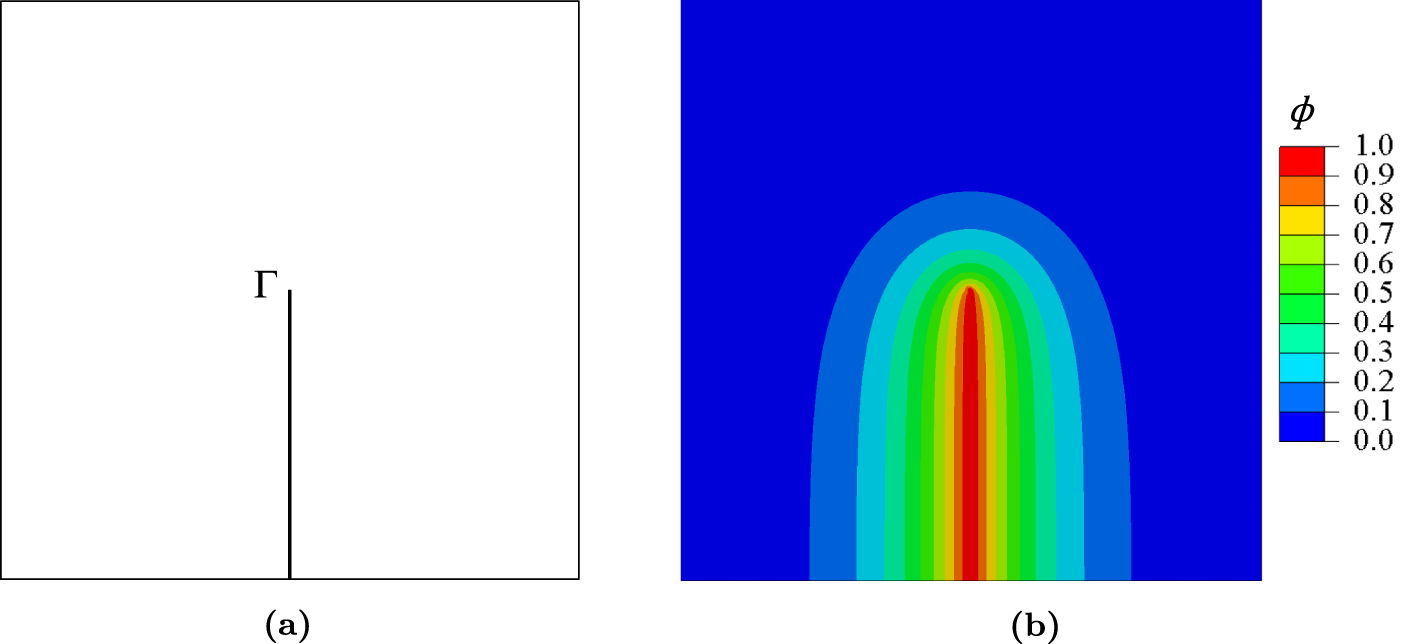
Figure 2: Phase-field regularisation of the discrete crack surface Γ: (a) Discrete crack surface Γ; (b) Regularised discrete crack surface Γ.

This regularisation of the sharp crack is achieved through the use of the crack surface density function γ [50] and the degradation function g [68]. The former ensures approximation of the sharp crack, while the latter gradually degrades the material, with both functions being governed by the PF parameter ϕ, which takes values between 0 (virgin material) and 1 (fully degraded material). Because of that, the internal part of the free energy functional is thus expressed as

Πint=Πb+Πs≈∫Ωg(ϕ)ψ+(ε(u))+ψ−(ε(u))dΩ+∫ΩGcγ(ϕ;∇ϕ)dΩ,(12)

allowing for the integration to be performed over the whole domain Ω, which was not possible in Eq. (11).

In contrast to the weak form, the strong form of the PF fracture formulation is more complex, and is defined using a system of equations

[g(ϕ)∇⋅σ++∇⋅σ−]+b=0,in Ω,(13)

[g(ϕ)σ++σ−]⋅n−h=0,on ∂Ωh,(14)

ψ+(ε(u))dg(ϕ)dϕ+Gc(∂γ(ϕ;∇ϕ)∂ϕ−∇⋅∂γ(ϕ;∇ϕ)∂∇ϕ)=0,in Ω,(15)

Gc∂γ(ϕ;∇ϕ)∂∇ϕ⋅n=0,on ∂Ω.(16)

where the plus/minus sign in the superscript indicates the positive/negative part of the specific quantity. This decomposition is necessary as it ensures physical behaviour, i.e., prevents the formation and propagation of cracks under compression, and needs to be performed for the material stiffness tensor C as well. Different techniques exist for this purpose. Most notably spectral decomposition [50], volumetric-deviatoric decomposition [69], no-tension decomposition [70] and directional stress decomposition [71].

In most cases, as it is in the presented work, the degradation function is represented using a second-order polynomial, i.e., g(ϕ)=(1−ϕ)2. Similarly, the crack surface density function γ can also be expressed in different ways [1]. Herein, it is defined following [50]

γ(ϕ,∇ϕ)=12(1lϕ2+l∇ϕ⋅∇ϕ),(17)

where l defines a length-scale parameter—a scalar value which controls the width of the diffusive layer. When l→0, a discrete crack surface Γ is recovered.

The PF method has experienced great success in modelling material damage and fracture in both brittle [55,58,59,72,73] and ductile materials [52,53,58,74]. In the former, the total strain energy density ψ is influenced only by the elastic small strain tensor εe, ensuring simple formulation of the body’s bulk energy Πb

Πb=∫Ω[g(ϕ)ψe+(εe)+ψe−(εe)]dΩ,(18)

while in the latter the total strain energy density ψ, as well as total small strain tensor ε, can be additively decomposed into plastic and elastic part. Because of that, the PF ductile formulation branches into two different approaches. In the first approach, the plastic part of the body’s bulk energy is not affected by the PF crack growth

Πb=∫Ω[g(ϕ)ψe+(εe)+ψe−(εe)+ψp(εp)]dΩ,(19)

while in the second, which is used in this work, both elastic and plastic parts of the body’s bulk energy are affected by the PF crack growth

Πb=∫Ω[g(ϕ)ψe+(εe)+ψe−(εe)]dΩ+∫Ωgp(ϕ)ψp(εp)dΩ,(20)

where gp stands for plastic degradation function which is also defined through a second-order polynomial as the standard degradation function g. For more details on different PF ductile fracture implementations, see Alessi et al. [75].

In terms of numerical implementation, the PF method offers a straightforward coupling with the finite element method since along the displacement field u, the PF variable ϕ becomes another quantity that is represented with the help of shape functions Ni and nodal values in each node i.

Obtaining the solution of the matrix system of equations can be achieved using either monolithic or staggered approach. In the monolithic approach, the system of equations is fully coupled, i.e., the values of the global displacement vector V and the global PF vector Φ are obtained simultaneously—in one iteration. However, due to a non-convex total free energy function Π, monolithic solvers can exhibit significant convergence issues, especially during the process of crack propagation. In contrast, a staggered scheme is characterised by a decoupled system of equations where solution vectors are obtained separately. The global displacement vector V in the iteration i+1 of the increment n is obtained as

Vni+1=Vni−KVV⋅RV,(21)

while for the PF part of the simulation the following is true

Φni+1=Φni−KΦΦ⋅RΦ.(22)

Global stiffness matrices KVV and KΦΦ, as well as the global residual vectors RV and RΦ are obtained from their local counterparts which are defined through

rv=∫Ωg(ϕ)BvTσdΩ−∫ΩNvTbdΩ−∫∂ΩNvThd∂Ω,(23)

rϕ=∫Ω[NϕT(ℋ(t)dg(ϕ)dϕ+Gclϕ)+GclBϕTBϕϕ]dΩ,(24)

kvv=∂rv∂v=∫Ωg(ϕ)BvTCBvdΩ,(25)

kϕϕ=∂rϕ∂ϕ=∫Ω[GclBϕTBϕ+NϕTNϕ(Gcl+ℋ(t)d2g(ϕ)dϕ2)]dΩ.(26)

with ℋ(t) being the strain energy density history field defined as

ℋ(t)=maxτ∈[0,t][ψe+(εe,t)+ψp(εp,t)],(27)

and N and B defining matrices of shape functions and shape functions derivatives, respectively.

The stability and robustness that come with staggered schemes are a significant advantage. This is especially important when damage in heterogeneous materials is in question. Although numerous staggered PF implementations exist, this work utilises the procedure proposed by Lesičar et al. [52]. For more details on monolithic and staggered schemes, see [76].

4  Multiscale Modelling of Damage and Fracture

4.1 Proposed Procedure

The proposed multiscale procedure for modelling damage and fracture in both brittle and ductile heterogeneous materials represents a synergy of the SCA and PF fracture formulation into one algorithm that combines the best features of the two methods. In it, the SCA and PF method each serve specific roles. The function of the SCA at the microlevel is to:

•   ensure computational efficiency by performing fast and accurate calculation of the RVE boundary value problem,

•   link two scales by performing first-order computational homogenization of the Cauchy stress tensor, material stiffness tensor, and strain energy density,

•   provide a straightforward extension to any type of constitutive law for a given material phase.

In contrast, the PF algorithm, which is present at the macrolevel, needs to:

•   cure pathological mesh dependence of the final results,

•   enable efficient and robust calculation of the macroscopic fracture processes,

•   provide additional stability and ensure objectivity by being present at the macrolevel instead of the microlevel.

It is important to note that the proposed procedure requires both Gc and l to be known a priori, since the calculation of damage is performed exclusively at the macrolevel. Because of that, Gc as well as l are treated as the macroscopic properties of the heterogeneous material and, from now on, will be designated as G¯c and l¯.

Although it operates under the assumption of small strains, the nature of the developed framework allows for the extension to model fracture at finite strains. The PF algorithm, as well as the SCA, represent flexible procedures which are not bound only to small strains configuration. Not only that, but the Lippmann-Schwinger equation, which is the basis of the SCA, is applicable to any physical problem that can be defined by elliptic partial differential equations. This includes problems of thermal conduction, electrical conduction, electromagnetism and many others. Ultimately, this opens up the possibility of tackling multiphysics problems, where fracture is influenced by multiple fields [77].

4.2 Methodology

Having described the main characteristics and aspects, the algorithmic implementation of the concurrent procedure is given in the Box 1, but also more vividly represented through Fig. 3.

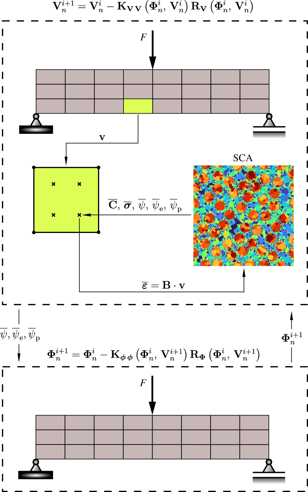
Figure 3: Proposed multiscale procedure algorithm.

Box 1: Concurrent multiscale damage algorithm for the increment n.

As can be seen from Box 1 and Fig. 3, the whole procedure requires two layers of finite elements. The first layer (also the starting layer) allows for the calculation of the displacement vector in each finite element, while the second layer performs PF analysis and therefore stores the value of the PF variable in each element.

Macroscopic values of the Cauchy stress tensor σ¯ and the material stiffness tensor C¯ are obtained directly from the SCA, which is present at the microlevel. These values are necessary for the first layer of elements, as the displacement finite element analysis requires the formation of the displacement stiffness matrix, using Eq. (25), and the displacement internal force vector, using Eq. (23), at each integration point of each element. Alongside macroscopic material stiffness tensor C¯, Eq. (25) also requires the information on the phase-field variable ϕ itself, which is the product of the analysis at the second layer of elements. However, at the beginning of every analysis, for each finite element, ϕ is equal to zero. This gives the value of 1 for the degradation function g and therefore ensures intact (virgin) material at the beginning of the simulation. Alongside macroscopic Cauchy stress tensor and macroscopic material stiffness tensor, the SCA also calculates macroscopic values of the total strain energy density ψ¯ as well as its elastic ψ¯e but also plastic ψ¯p part. These values are not used in the first layer of elements as they are sent to the second layer of elements, since they are required by the PF analysis.

In contrast to the total number of five output variables, the SCA requires only one input variable, more precisely the macroscopic small strain tensor ε¯ or the macroscopic Cauchy stress tensor σ¯. In one iteration, the SCA needs to be called e⋅j times, where e represents the total number of finite elements, while j stands for the total number of integration points in the finite element.

In the second layer of elements, the PF fracture formulation algorithm relies on the macroscopic values of the total strain energy density, plastic strain energy density and elastic strain energy density to formulate the PF stiffness matrix, defined by Eq. (26), and the PF internal force vector which is calculated using Eq. (24). To be more precise, formation of both PF stiffness matrix as well as PF internal force vectors is performed using strain energy density history field ℋ defined by Eq. (27). Definition of strain energy density history field ℋ stems directly from the description of the body’s bulk energy Πb in Eq. (20), ensuring participation of only positive part of the elastic strain energy density as well as thte total plastic strain energy density; however, only if the material exhibits elastoplastic behaviour. When the body is loaded fully by tension, no energy decomposition is needed. In that case, the total strain energy density is enough to determine the strain energy density history field. However, in the case of complex loading, strain energy density decomposition is needed, and is performed only on the elastic part. Recall that the values of the macroscopic length scale parameter l¯ as well as the critical value of the energy release rate G¯c are prescribed in advance and are used in each integration point of each element through Eqs. (24) and (26). After the formation of the global system, the global phase-field vector Φn in the current increment n is obtained. Its values are then used in the first layer of elements for the calculation of the degradation function g, which participates in the formation of the displacement stiffness matrix.

The described procedure is performed iteratively between the two layers until the equilibrium in both layers is achieved. The number of required iterations is primarily driven by the level of degradation the heterogeneous material has sustained. This is particularly true in the case of rapid crack propagation in brittle fracture, where the total number of iterations often climbs above 1000 and therefore leads to long computational time. Utilisation of the line search algorithm [78] or the Broyden–Fletcher–Goldfarb–Shanno (BFGS) Quasi-Newton method [79] can improve convergence and therefore lead to the need for fewer iterations. Since the presented framework is based on a staggered PF scheme [52], utilisation of the BFGS method does not represent a sensible choice as it is primarily used in a monolithic PF scheme [79]. A line search assisted algorithm, on the other hand, is integrated into the presented framework, improving convergence and adding an additional layer of numerical stability. For more information on the convergence of the phase-field method, see [52,77,79].

The described concurrent framework ensures a high level of computational efficiency by utilising SCA at the microlevel, prevents numerical instability by removing calculation of damage from the microlevel and prevents pathological mesh dependence at the macrolevel by employing a non-local continuum damage model, i.e., PF. However, these improvements do not come free of charge. Since the framework intentionally avoids numerical analysis of damage and fracture at the microlevel, information on micro crack initiation and propagation, as well as void coalescence, is not present in any form. Moreover, the macroscopic value of the length-scale parameter l¯ as well as the macroscopic value of the critical energy release rate G¯c needs to reflect the overall behaviour of the microstructure in question, and must be calculated from the information of the length-scale parameter and the critical value of energy release rate of each microconstituent. The accurate and effective determination of both l¯ and G¯c does not represent a trivial task. Therefore, this study does not attempt to compute these quantities and instead adopts prescribed values for them.

Although the k-means clustering and the formation of interaction tensor DIJ are performed in the commercial software Matlab [80], the finite element procedure described above is fully implemented in the commercial finite element software Abaqus [81] with the help of user subroutines.

5  Numerical Examples

5.1 Test Setup

The performance of the implemented concurrent approach is assessed using two different 2D and 3D microstructures, which are depicted in Fig. 4, and four different geometrical specimens, which are shown in Fig. 5. The microstructures in question are a 2D unit cell, a 3D unit sphere, a complex 2D RVE and a complex 3D RVE. The geometry of both 2D and 3D complex microstructures is coming directly from the statistical analysis of the experimental metallography of nodular cast iron that was produced by the Tundish method of casting, as explained in [82]. All four samples consist of two material phases-matrix and inclusion. The volume fraction of a single inclusion is 12.5%, for a 2D unit cell, i.e., 11.3% for a 3D unit sphere. In contrast, the volume fraction of elliptical inclusions in 2D and 3D complex RVEs are 7.6% and 3.5%, respectively. For simplicity, the dimension of an edge in both 2D unit cell and 3D unit sphere is 1 millimetre, while the edge length in the case of a complex 2D RVE is equal to 0.5 millimetres, i.e., 0.2 millimetres for the case of a complex 3D RVE.

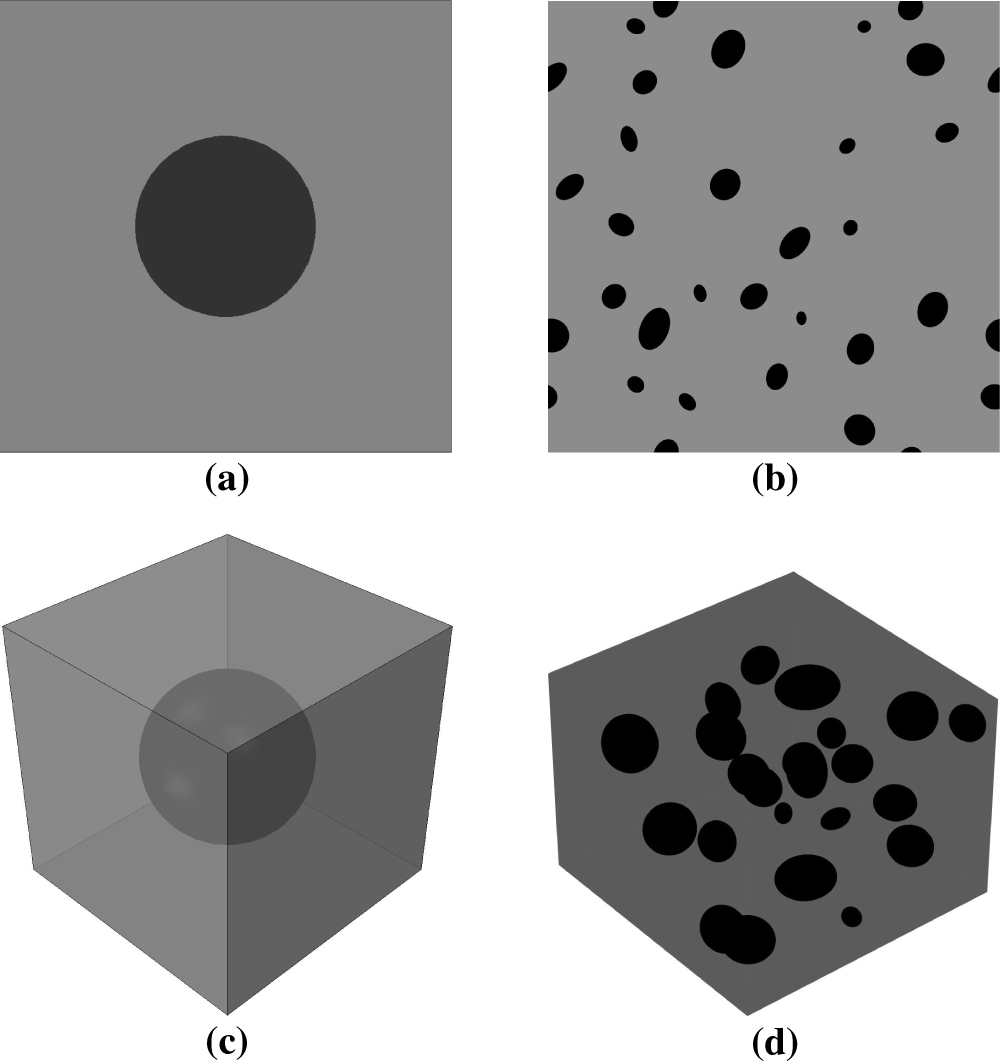
Figure 4: Microstructural samples: (a) 2D unit cell geometry; (b) 3D unit sphere geometry; (c) Complex 2D RVE; (d) Complex 3D RVE.

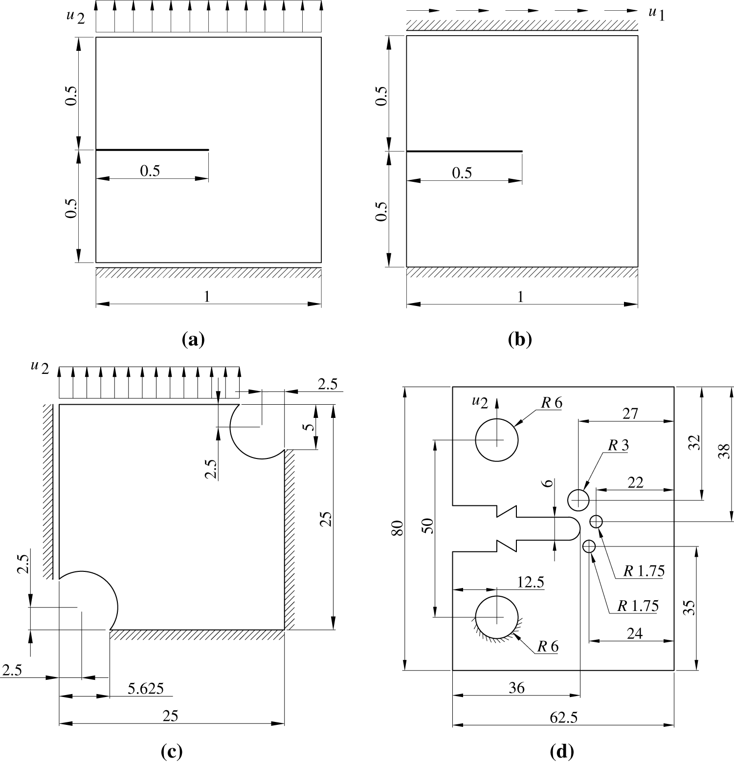
Figure 5: Test specimens: (a) Single-edge notched plate-pure tension loading; (b) Single-edge notched plate-pure shear loading; (c) Double-notched specimen; (d) Sandia fracture challenge specimen.

On the other hand, test specimens in Fig. 5 represent frequently used samples for numerical evaluation of fracture algorithms, with all dimensions being given in millimetres. Notice that for all four samples, only displacement-type boundary conditions are applied, implying the presence of only macro-strain constraints in the calculation of the RVE boundary value problem. Last but not least, when three-dimensional analysis is in question, the thickness of the three samples is 0.1 millimetres for the single-edge notched plate [50], 10 millimetres for the double-notched specimen [17] and 2 millimetres for the Sandia fracture challenge specimen [53].

With the definition of all test microstructures and all test specimens, the testing procedure can now be specified. It consists of two stages, and in each stage, both brittle and ductile fracture (with the assumption of small strains) are considered.

The first or initial stage of testing will focus on the proposed algorithm’s accuracy and computational efficiency. This part of numerical testing includes analysis of a 2D unit cell and a 3D unit sphere (for both brittle and ductile fracture) with two different material configurations. The first material configuration essentially forms a homogeneous material, as both the matrix and one inclusion possess equivalent mechanical properties. The aim is to show that both SCA and DNS (performed with homogeneous material properties) will give almost identical results since no material heterogeneity exists. The second material configuration downgrades, by 5%, some mechanical properties of the inclusion. Now, the goal is to demonstrate that there will be a difference in force-displacement response, as the material heterogeneity is present in the microstructure. The mechanical properties chosen for the first, i.e., second material configuration are given in Table 1.

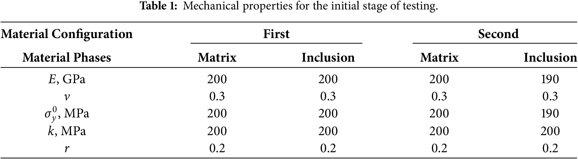
As can be seen from Table 1, in the second material configuration both modules of elasticity E and initial yield strength σy0 of the inclusion are degraded by 5%, while the Poisson ratio ν and two material parameters of the Swift’s non-linear isotropic hardening law σy=σy0(1+kεeqp)r are identical in both configurations. It is important to clarify that in the case of brittle fracture, both matrix and inclusion are treated as linearly elastic material, in contrast to ductile fracture, where both material phases are described using the von Mises plasticity model.

Complex RVEs depicted by Fig. 4 will serve to evaluate the robustness and stability of the proposed concurrent procedure, which is the subject of the second stage of testing. Random geometrical configuration of inclusions will produce a highly nonuniform distribution of stress and strain fields, thus ensuring an appropriate level of complexity. As was the case in the first stage of testing, both brittle and ductile fracture (assuming small strains) is considered; however, inclusions (in all analyses) are treated as linearly elastic material. Mechanical properties of the elastoplastic matrix correspond to those from [1], and their values are

E=228.9 GPa, ν=0.282,σy0=246.67 MPa, k=117.95,r=0.208,(28)

while the mechanical behaviour of inclusions is modelled by means of material properties of isotropic graphite [83]

E=25.5 GPa, ν=0.312.(29)

In addition to multiscale phase-field analysis, the second stage also includes DNS analysis using homogeneous properties of the complex RVE. Homogeneous properties of the microstructures shown in Fig. 4b,d can be obtained by running a simple concurrent multiscale analysis using one linear macroscopic finite element with four (in 2D) and eight (in 3D) nodes. The element needs to be subjected to a uniaxial tension to ensure a homogeneous state of the macroscopic stress and strain tensor, while the total mechanical response of the element is governed by the analysis and homogenization of the complex RVE boundary value problem. From the obtained macro stress-strain curve it is possible to calculate the macro values of: modulus of elasticity E¯, Poisson ratio ν¯, initial yield strength σ¯y0, Swift’s law parameter k¯ and Swift’s law parameter r¯. For the 2D complex RVE depicted in Fig. 4b the homogeneous properties are

E¯=195.1 GPa, ν¯=0.2815,σ¯y0=248.9 MPa, k¯=44.7468 MPa, r¯=0.48836,(30)

while for the 3D complex RVE depicted by Fig. 4d the homogeneous properties are equal to

E¯=216 GPa, ν¯=0.28,σ¯y0=252.8 MPa, k¯=51.3573 MPa, r¯=0.3865.(31)

It is also necessary to define phase-field fracture parameters, namely the length-scale parameter l¯ and the critical value of the energy release rate (critical Griffith force) G¯c. Recall from Section 4.2 that the value of both length-scale parameter l¯ and the critical Griffith force G¯c need to be defined a priori, i.e., they are not the product of the analysis at the microlevel. As well as the values given in Table 1, values of both l¯ and G¯c have a direct impact on the overall mechanical behaviour and cannot be chosen randomly.

For the case of brittle fracture in the first stage of testing, the critical value of Griffith force is taken to be 2.7 N/mm, while its value in the problems of ductile fracture is equal to 29.7 N/mm. The value of 2.7 N/mm is present in many contributions where analysis of PF fracture in brittle or quasi-brittle materials is considered [50–52,59]. On the other hand, 29.7 N/mm simply represents an increase of 11 times from 2.7 N/mm, as ductile materials have significantly higher values of critical energy release rate. For the case of a complex RVE, the values of critical Griffith force for brittle and ductile fracture are 1.2957 N/mm [84], i.e., 86.0 N/mm [82], respectively. The former represents a value of G¯c for a high-carbon martensitic steel, while the latter is the value of G¯c of the nodular cast iron. The defined values are fixed and are not (in any way) dependent on the type of geometrical specimen.

In contrast to G¯c, l¯ represents both material and geometrical property as it relates to the type of material but also the dimensions of the domain which is being analysed. Decreasing the value of this parameter leads to improved approximation of the discrete crack; however, it also results in the need for a fine element mesh in the region of crack initiation and propagation [50,51]. An increase in the overall number of finite elements at the macrolevel undoubtedly increases the computational complexity of the concurrent multiscale approach. From their own experience, authors have observed that the value of l¯ should be about 50 to 100 times smaller than the characteristic dimension of the body. This interval provides correct physical behaviour but also ensures an acceptable level of computational complexity.

Last but not least, a “quick check” before the multiscale concurrent analysis is performed in order to compare SCA and DNS (which is conducted using FEM) for all four microstructural samples. Tests are carried out under two different macro-strain constraints—pure shear and pure hydrostatic loading, since these constraints represent a problematic type of macroscopic constraints for the SCA. The material properties of a 2D unit cell, as well as the 3D unit sphere, match those from the second material configuration presented in Table 1, while their values in the case of complex RVEs are given by Eqs. (28) and (29). Results of the k-means clustering analysis are depicted in Figs. 6–9, while diagrams of macroscopic stress-strain relations can be seen in Figs. 10–13.

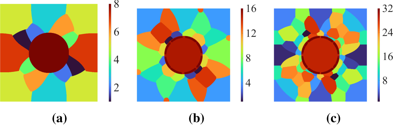
Figure 6: Results of the k-means clustering for a 2D unit cell: (a) k=8; (b) k=16; (c) k=32.

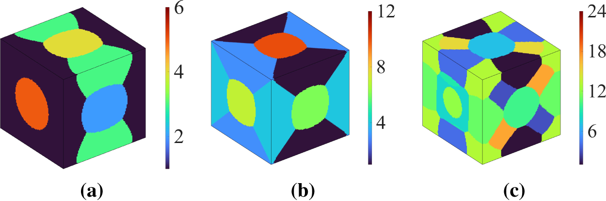
Figure 7: Results of the k-means clustering for a 3D unit sphere: (a) k=6; (b) k=12; (c) k=24.

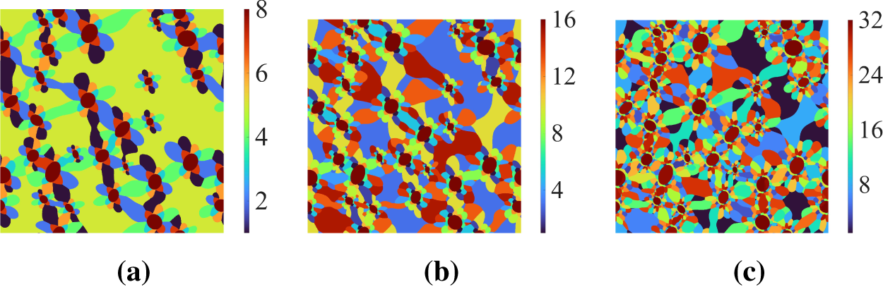
Figure 8: Results of the k-means clustering for a complex 2D RVE: (a) k=8; (b) k=16; (c) k=32.

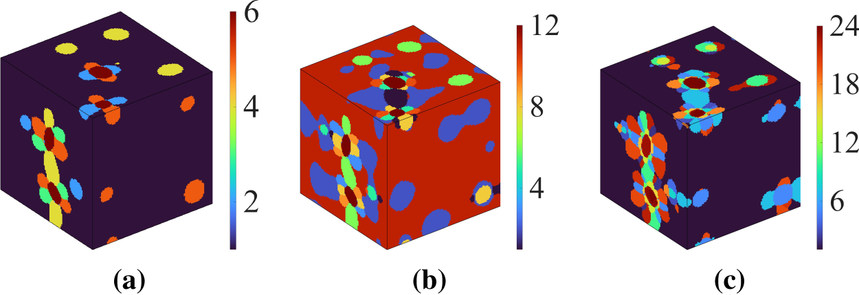
Figure 9: Results of the k-means clustering for a complex 3D RVE: (a) k=6; (b) k=12; (c) k=24.

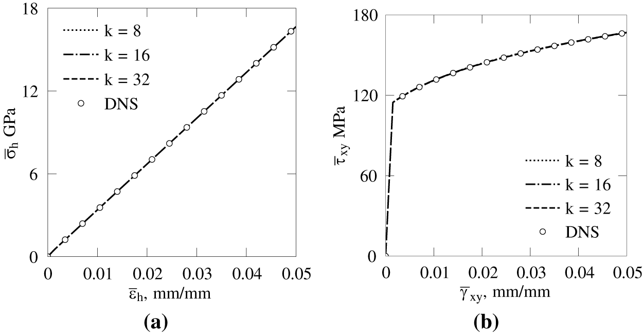
Figure 10: Comparison of the macroscopic results for a 2D unit cell: (a) Hydrostatic loading; (b) Shear loading.

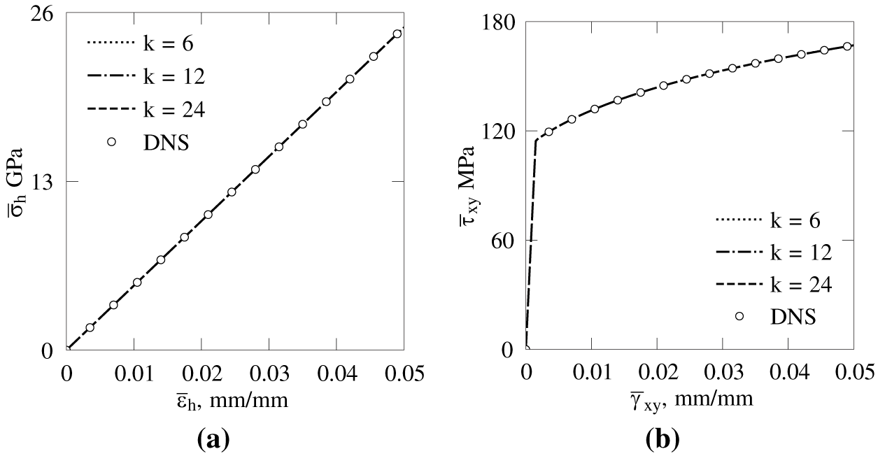
Figure 11: Comparison of the macroscopic results for a 3D unit sphere: (a) Hydrostatic loading; (b) Shear loading.

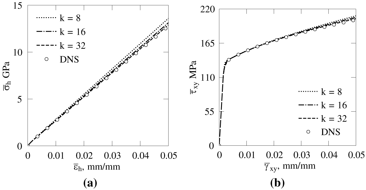
Figure 12: Comparison of the macroscopic results for a complex 2D RVE: (a) Hydrostatic loading; (b) Shear loading.

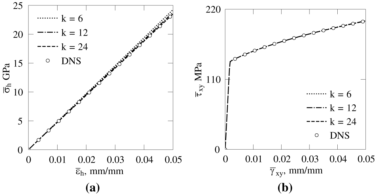
Figure 13: Comparison of the macroscopic results for a complex 3D RVE: (a) Hydrostatic loading; (b) Shear loading.

Cluster decompositions provided by Figs. 6–9 show that each microstructural sample is decomposed with three different cluster discretisations, each being two times finer than the previous one. The starting number of material clusters for a 2D unit cell and the 2D complex RVE is 8, while 6 represents the initial discretisation for a 3D unit sphere, i.e., the 3D complex RVE. The choice of the number of material clusters k does not follow a strict rule, as it is problem-dependent and heavily based on experience. From the authors’ experience, k=8 (for 2D) and k=6 (for 3D) have proven to be appropriate starting points, while the increase by a factor of 2 represents a sensible choice since k−means clustering reduces the error by 50% each time the number of clusters increases fourfold.

Due to a simple geometry and similar mechanical properties, SCA is able to predict macroscopic response of the 2D unit cell, as well as the 3D unit sphere, with pinpoint accuracy for both hydrostatic and pure shear type of macroscopic constraints. This, unfortunately, is not possible for the case of a complex microstructures, as can be seen from Figs. 12 and 13. However, even with 8 material clusters, SCA is able to achieve satisfactory results, with the maximum error of “only” 6.5 % for the case of hydrostatic loading of a complex 2D RVE.

For the first stage of testing, decompositions with 8 (for a 2D unit cell) and 6 (for a 3D unit sphere) material clusters are used, while for the second stage of testing, decompositions with 8, i.e., 16 material clusters (for a complex 2D RVE) and 6, i.e., 12 material clusters (for a complex 3D RVE) are present. In both the first and the second stage, every analysis was executed using a single thread of an Intel Xeon E5-1620 (version 2) processor, which ensures an objective comparison of the CPU time needed to complete the analysis. All simulations are performed with a fixed increment size and using a projection-based scheme algorithm for the update of the reference material stiffness tensor C0. The projection-based scheme represents a more stable approach for finding the optimal values of Lamé parameters that form the stiffness of the reference homogeneous material. Moreover, the overall computational efficiency of the SCA is higher when a projection-based scheme is used instead of a regression-based scheme [1]. In addition to the actual CPU times, which were taken directly from the analysis, the first stage of testing also provides an approximated CPU time for an FE2 approach. This approximation is the result of using the average value of the SCA acceleration in contrast to DNS, and assumes that the DNS calculation of the RVE boundary value problem is performed on the 100 × 100 pixel grid using fully integrated linear quadrilateral plane strain elements in 2D, and 40 × 40 × 40 voxel grid using fully integrated linear hexahedral elements in 3D, and of course using one thread of the same Intel processor.

5.2 First Stage of Testing

This subsection includes results obtained by the DNS (with homogeneous material properties), the proposed concurrent approach with the first material configuration for the unit cell (“MS1”) and the proposed concurrent approach with the second material configuration for the unit cell (“MS2”). Each analysis includes the force-displacement diagram, alongside its zoomed-in view and images depicting the crack-phase field for both DNS and MS2 simulations. In addition to figures, each result is accompanied by a table of CPU time for all three analyses. Recall that one of the goals of this testing is to determine the computational efficiency of the proposed concurrent approach; therefore, comparing CPU times is not optional but mandatory. Results from the first six analyses are related to the brittle fracture, while the ductile fracture is present in the next four analyses. For every analysis, the total number of finite elements in the finite element mesh at the macroscale are given. The finite element mesh is always finer near the area of crack propagation, and following [50], the size of the finite element is at least two times smaller than the value of the macroscopic length-scale parameter l¯.

The first specimen to be tested is the 2D single-edge notched plate depicted in Fig. 5a. The model is discretised by 12,122 fully integrated linear quadrilateral plane strain elements. The chosen length-scale parameter is equal to 0.01 mm. The analysis is performed in 100 increments using no energy split. The results are presented in Fig. 14, and corresponding computational times are displayed in Table 2.

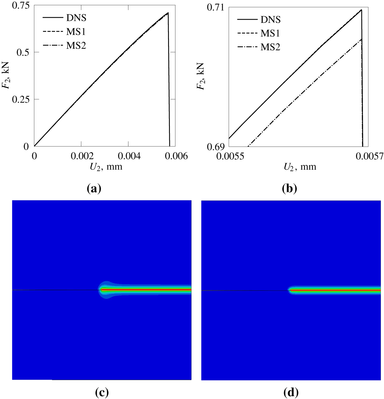
Figure 14: A 2D single-edge notched plate—pure tension loading: (a) Force-displacement curves; (b) Zoomed-in view; (c) Crack topology—DNS; (d) Crack topology—MS2.

A 2D single-edge notched plate is also present in the second example, although this time it is loaded by pure shear Fig. 5b. The model is discretised by 28,447 fully integrated linear quadrilateral plane strain elements. The chosen length-scale parameter is equal to 0.01 mm, and the analysis is performed using a volumetric-deviatoric energy split. The results are presented in Fig. 15, and corresponding computational times are displayed in Table 3.

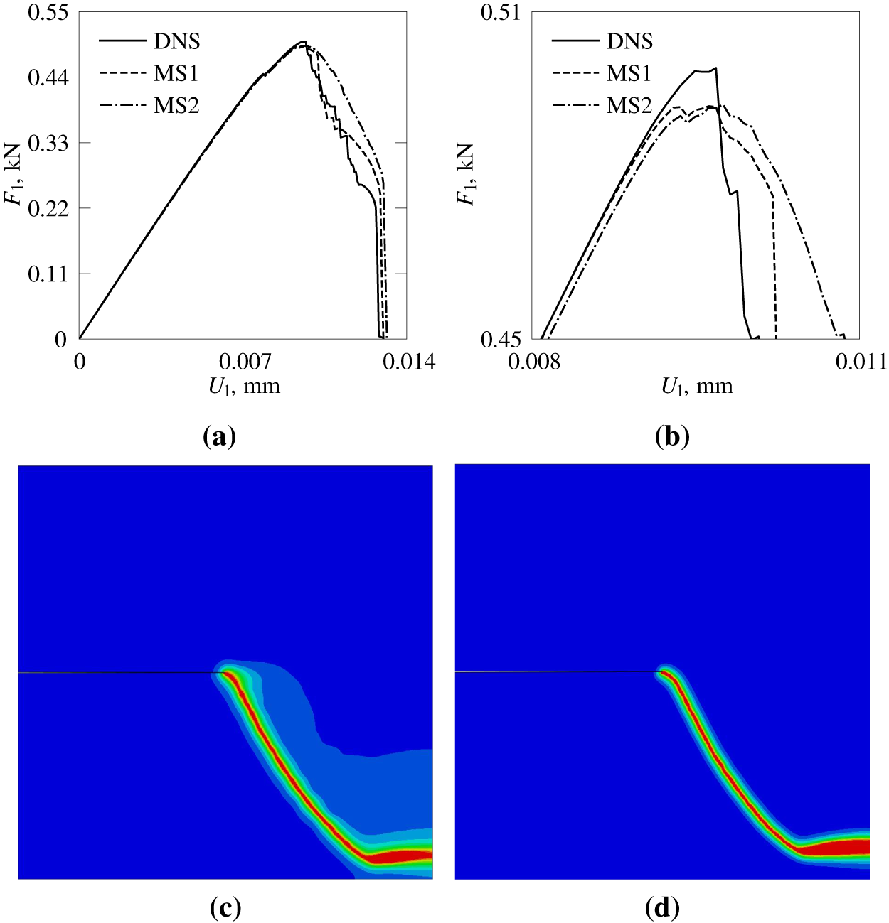
Figure 15: A 2D single-edge notched plate—pure shear loading (volumetric-deviatoric decomposition): (a) Force-displacement curves; (b) Zoomed-in view; (c) Crack topology—DNS; (d) Crack topology—MS2.

The third example is identical to the previous one, with the only difference being the utilisation of a spectral energy decomposition. Results, which again include force-displacement diagrams, crack topologies and CPU times, are visible in Fig. 16 and Table 4.

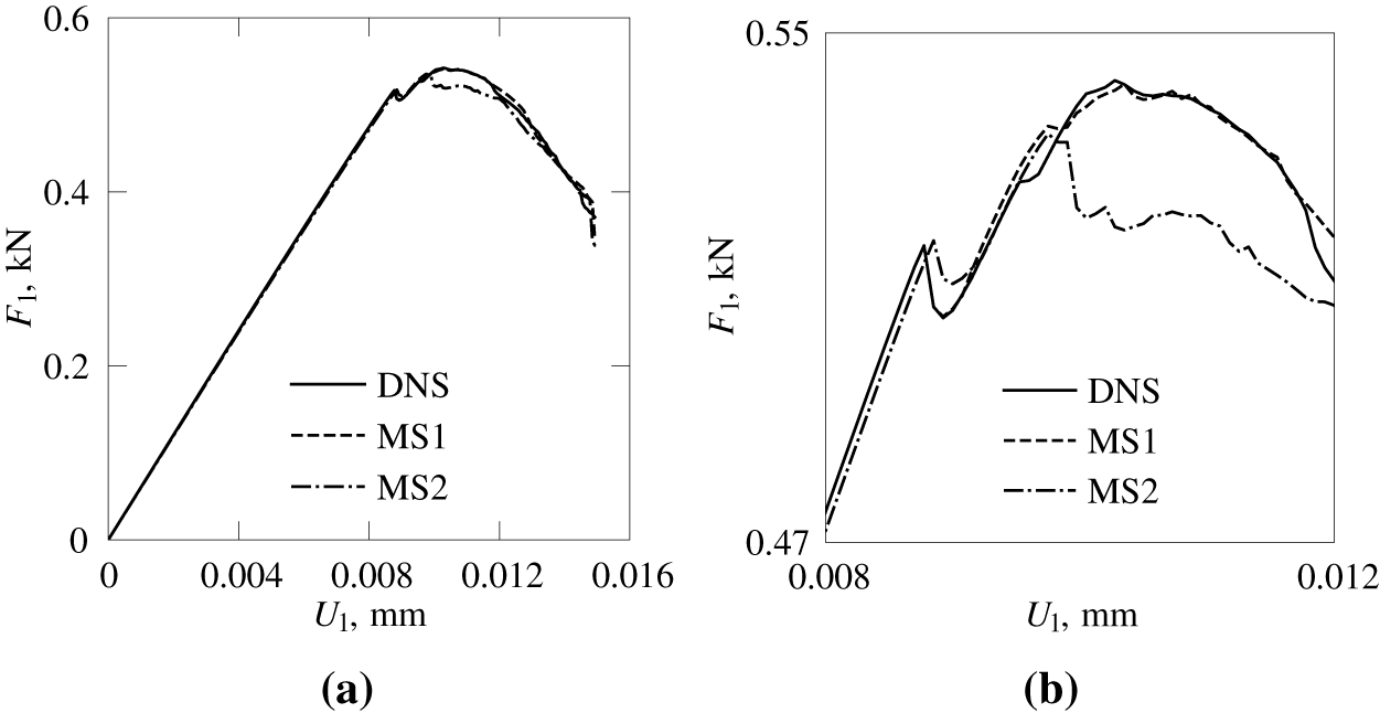
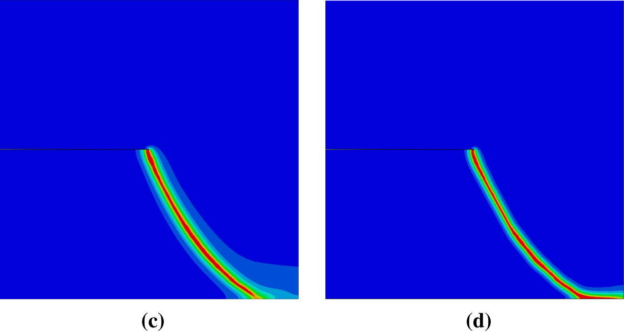
Figure 16: A 2D single-edge notched plate—pure shear loading (spectral decomposition): (a) Force-displacement curves; (b) Zoomed-in view; (c) Crack topology—DNS; (d) Crack topology—MS2.

The next example represents an extension of the first, i.e., a three-dimensional single-notched plate also loaded by tension. The model is discretised by 13,680 fully integrated linear hexahedral elements. The chosen length-scale parameter is equal to 0.01 mm. The analysis is performed in 100 increments using no energy split. The results are presented in Fig. 17, and corresponding computational times are displayed in Table 5.

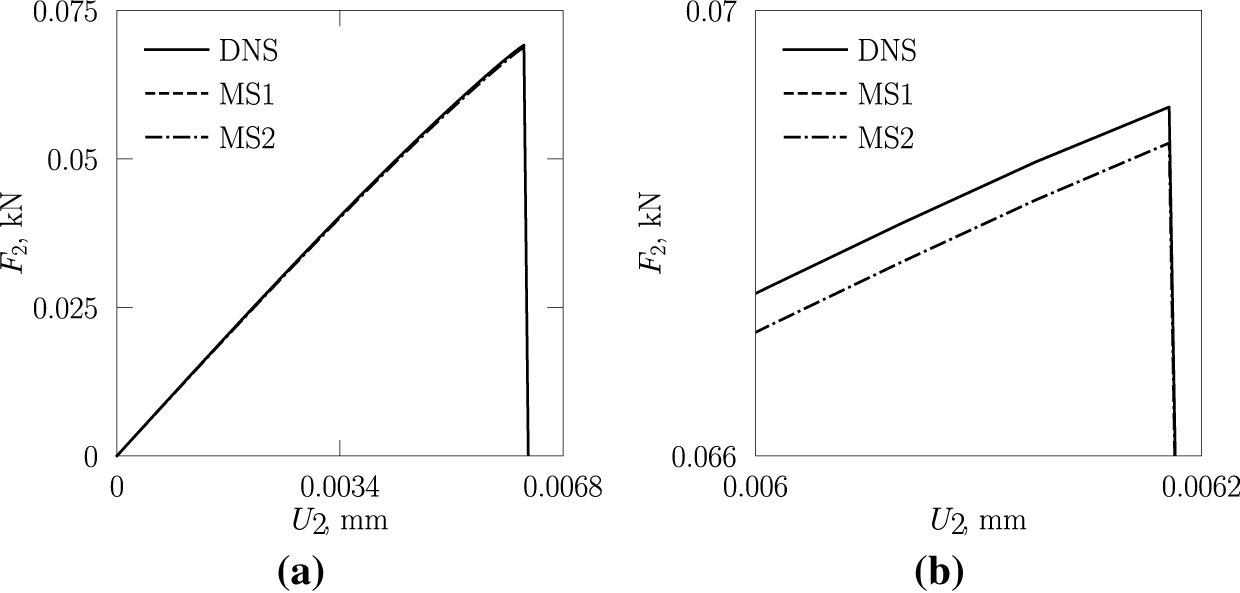
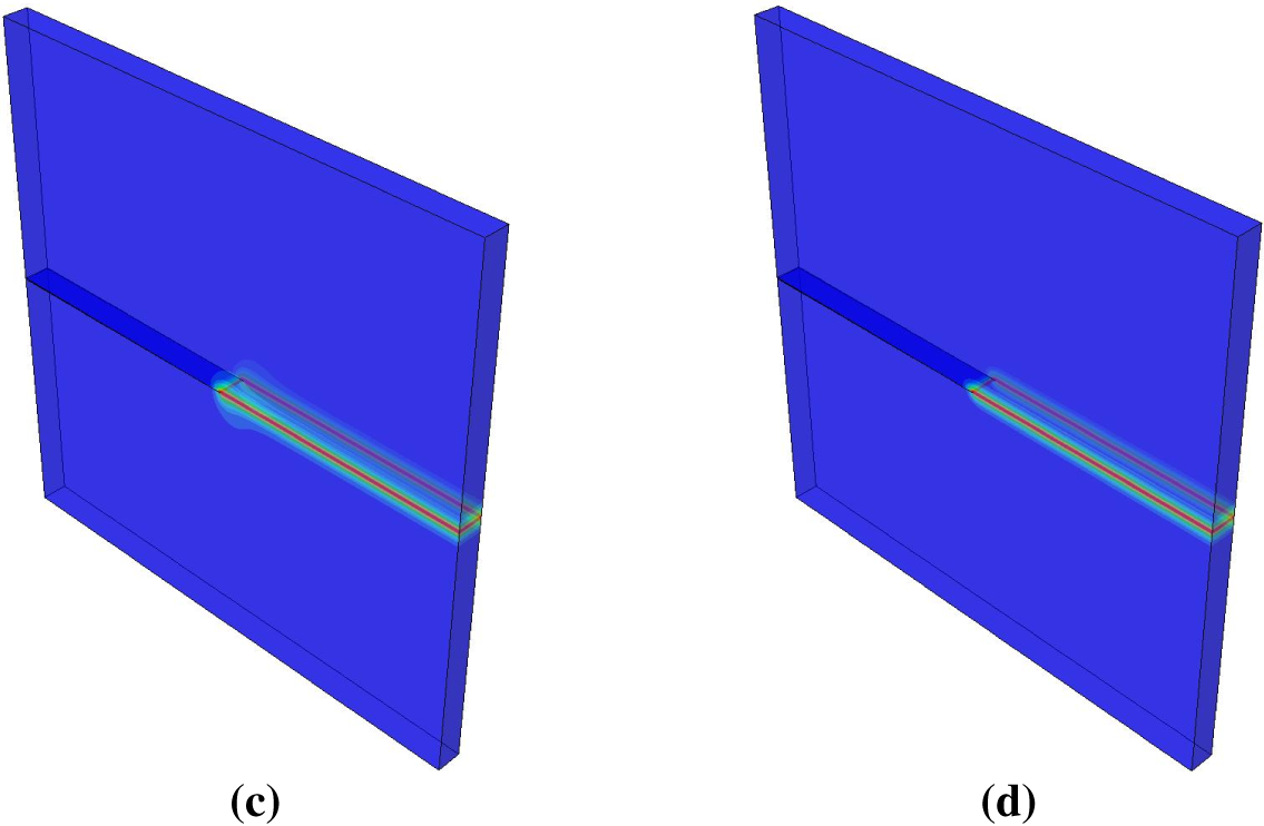
Figure 17: A 3D single-edge notched plate: (a) Force-displacement curves; (b) Zoomed-in view; (c) Crack topology—DNS; (d) Crack topology—MS2.

A 2D double-notched specimen Fig. 5c is next in line. The model is discretised by 22,127 fully integrated linear quadrilateral plane strain elements. The chosen length-scale parameter is equal to 0.3 mm. The analysis is performed in 100 increments using no energy split. The results are presented in Fig. 18, and corresponding computational times are displayed in Table 6.

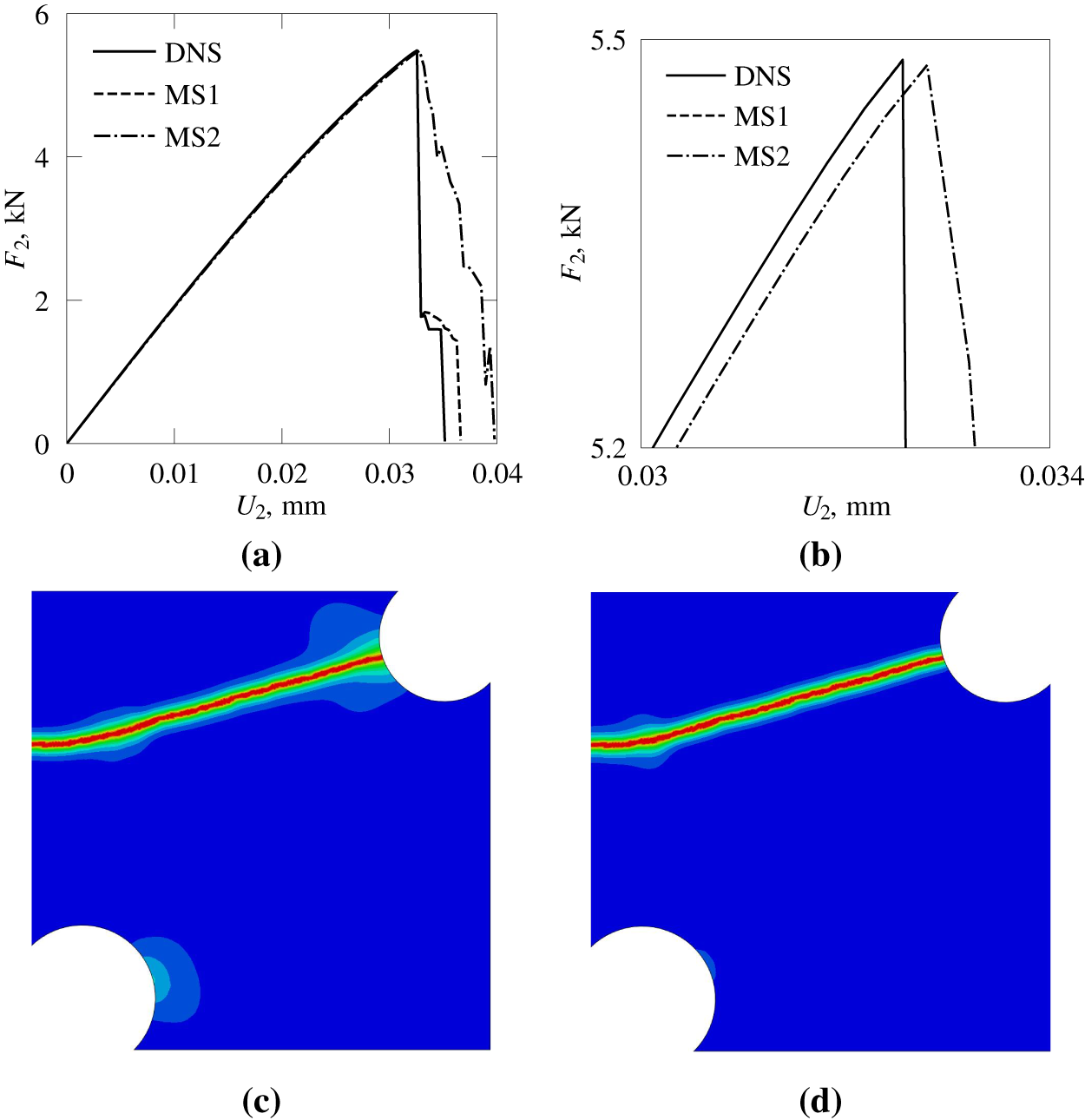
Figure 18: A 2D double-notched specimen (brittle fracture): (a) Force-displacement curves; (b) Zoomed-in view; (c) Crack topology—DNS; (d) Crack topology—MS2.

The results for the 3D double-notched specimen are depicted by Fig. 19 and Table 7. The model is discretised by 31,389 fully integrated linear hexahedral elements. The chosen length-scale parameter is equal to 0.3 mm. The analysis is performed in 100 increments using no energy split.

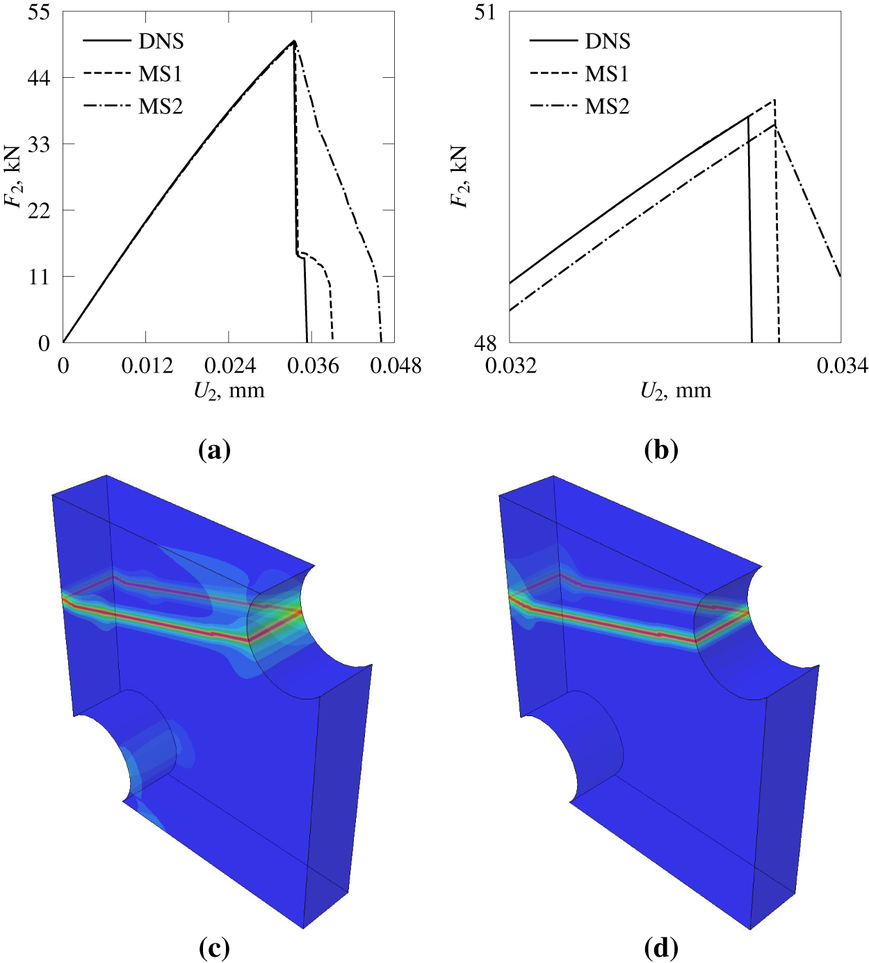
Figure 19: A 3D double-notched specimen (brittle fracture): (a) Force-displacement curves; (b) Zoomed-in view; (c) Crack topology—DNS; (d) Crack topology—MS2.

As in the case of brittle fracture, a 2D double-notched specimen Fig. 5c is also present in ductile fracture analysis. The model is discretised by 16,988 fully integrated linear quadrilateral plane strain elements. The chosen length-scale parameter is equal to 0.6 mm. The analysis is performed in 200 increments using no energy split. The results are presented in Fig. 20, and corresponding computational times are displayed in Table 8.

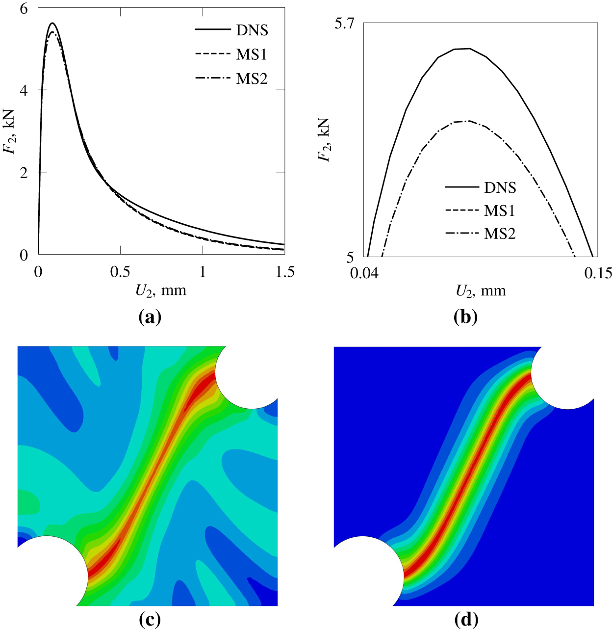
Figure 20: A 2D double-notched specimen (ductile fracture): (a) Force-displacement curves; (b) Zoomed-in view; (c) Crack topology—DNS; (d) Crack topology—MS2.

The results for the 3D double-notched specimen (in the case of ductile fracture) are shown by Fig. 21 and Table 9. The model is discretised by 20,757 fully integrated linear hexahedral elements. The chosen length-scale parameter is equal to 0.6 mm. The analysis is performed in 200 increments using no energy split.

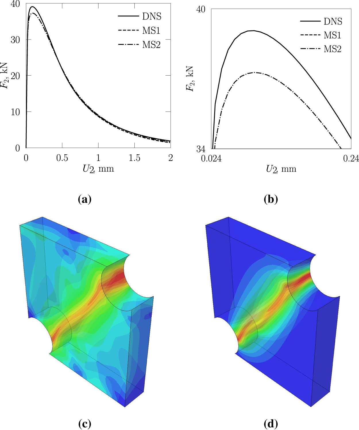
Figure 21: A 3D double-notched specimen (ductile fracture): (a) Force-displacement curves; (b) Zoomed-in view; (c) Crack topology—DNS; (d) Crack topology—MS2.

A 2D Sandia fracture challenge specimen Fig. 5d is the last example in 2D plane strain ductile fracture tests. The model is discretised by 18,589 fully integrated linear quadrilateral plane strain elements. The chosen length-scale parameter is equal to 0.4 mm. The analysis is performed in 200 increments using volumetric-deviatoric energy split. The results are presented in Fig. 22, and corresponding computational times are displayed in Table 10.

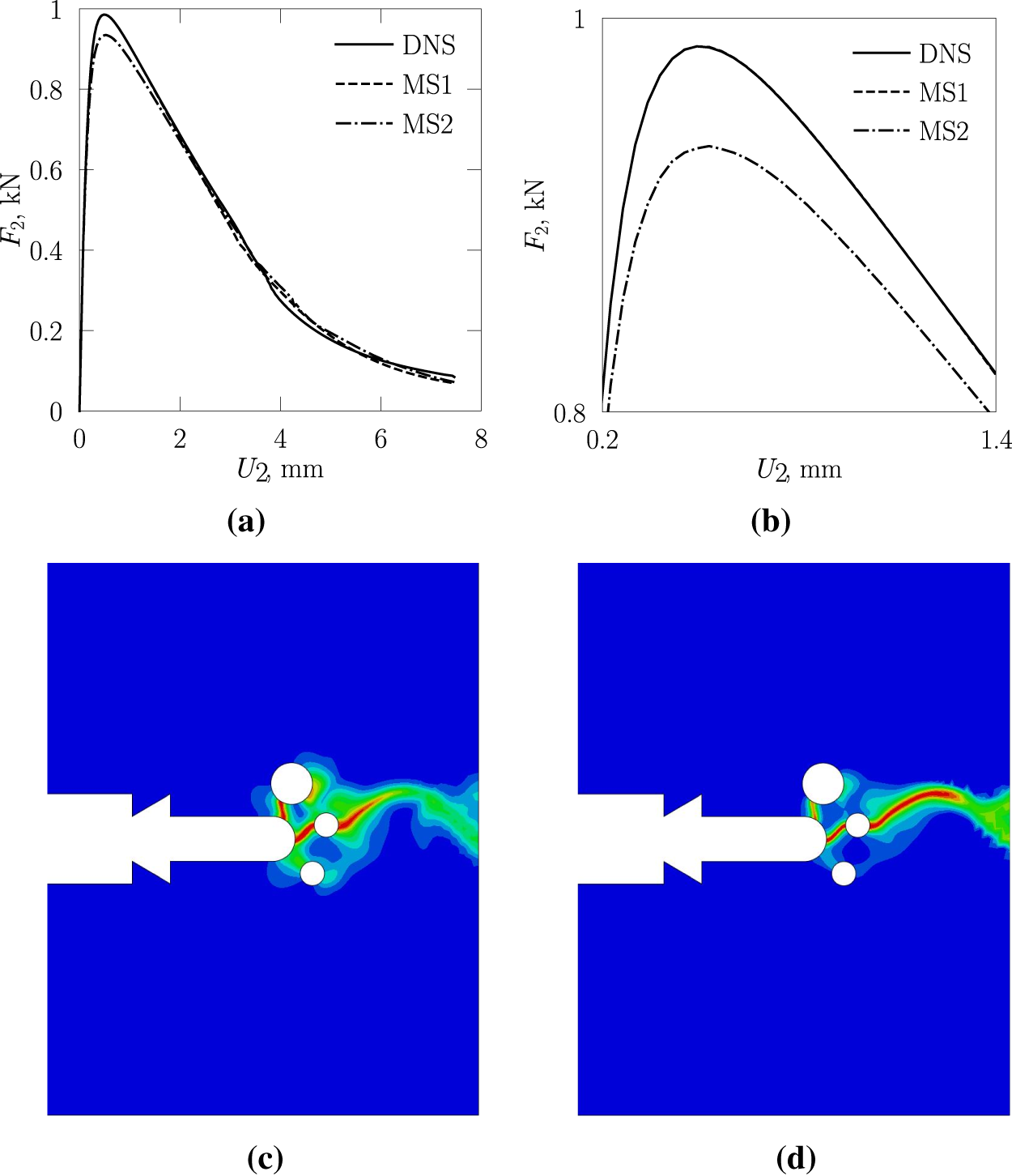
Figure 22: A 2D Sandia fracture challenge specimen: (a) Force-displacement curves; (b) Zoomed-in view; (c) Crack topology—DNS; (d) Crack topology—MS2.

The first stage of testing is concluded with the 3D Sandia fracture challenge specimen. The model is discretised by 35,241 fully integrated linear hexahedral elements. The chosen length-scale parameter is equal to 0.4 mm. The analysis is performed in 200 increments using volumetric-deviatoric energy split. The results are presented in Fig. 23, and corresponding computational times are displayed in Table 11.

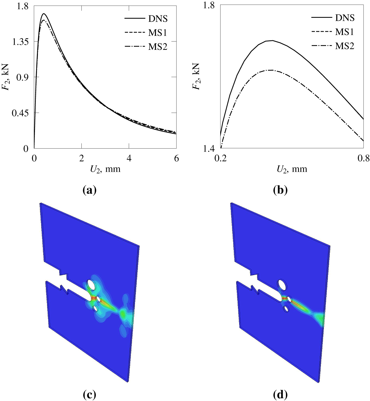
Figure 23: A 3D Sandia fracture challenge specimen: (a) Force-displacement curves; (b) Zoomed-in view; (c) Crack topology—DNS; (d) Crack topology—MS2.

From the figures and tables displayed in the previous few pages, it can be concluded that the proposed concurrent procedure is able to describe fracture in both brittle and ductile materials in an accurate and computationally efficient way. Force-displacement diagrams and their zoomed-in views show that there exists almost no difference between DNS analysis (performed using homogeneous material properties) and the developed concurrent approach performed with the material properties defined by the first material configuration.

On the other hand, when the module of elasticity E, i.e., initial yield strength σy0 (of the inclusion) is degraded by 5%, the developed concurrent procedure gives slightly different results, as expected. All zoomed-in views show that the value of peak force is always the lowest for the heterogeneous microstructure (MS2), which is particularly noticeable when fracture in ductile heterogeneous material is in question. This result is important, as it validates the accuracy and provides proof that the proposed concurrent approach gives correct results.

Figures that depict the crack topology for both DNS and MS2 are also in excellent agreement. Crack paths are more than similar, which is again an important result as it provides additional confirmation of the validity of the developed concurrent procedure. Interestingly, the crack topology figures show that the concurrent approach produces a more localised distribution of the crack phase-field parameter ϕ in contrast to the DNS approach.

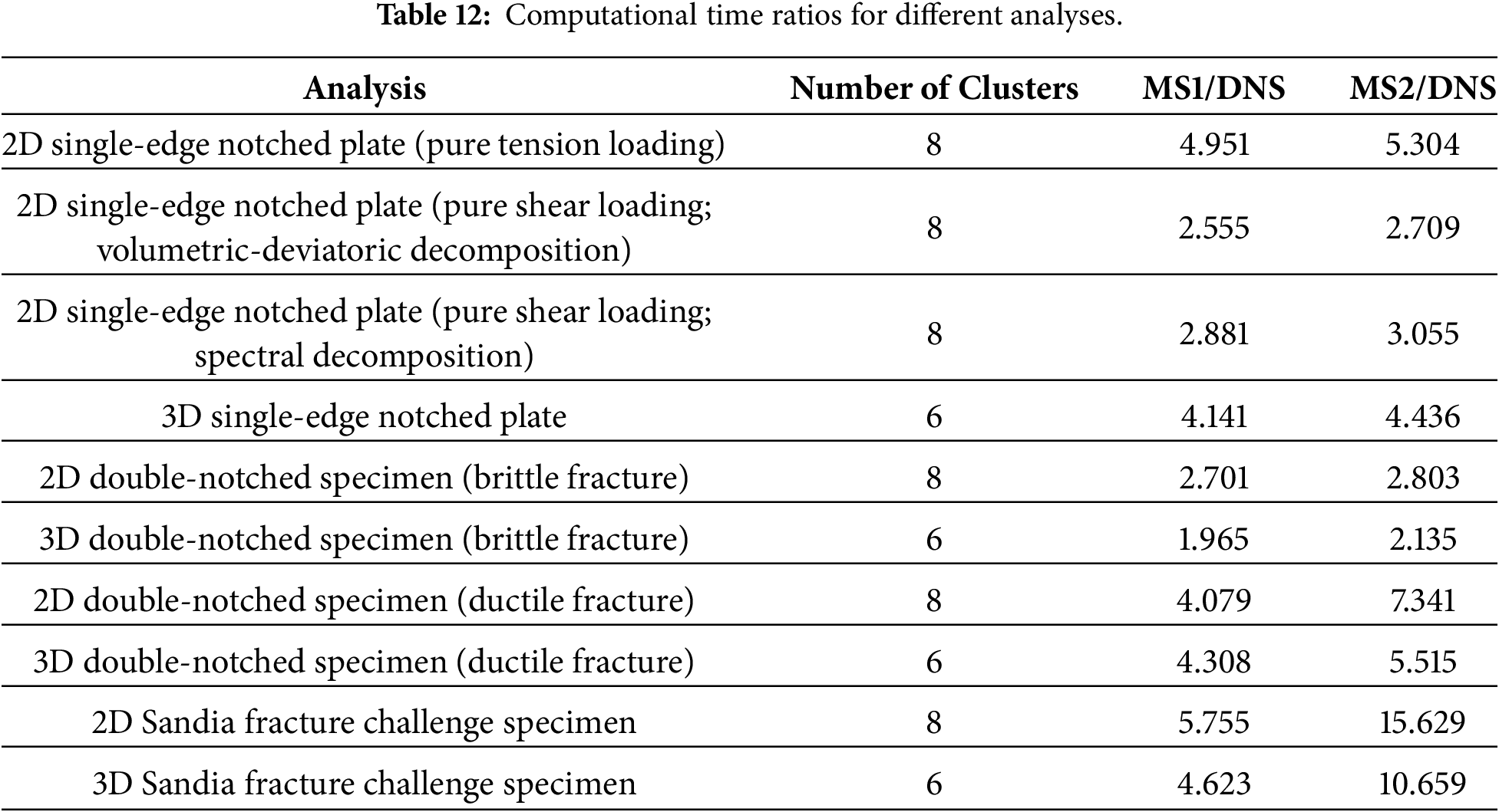
In addition to being accurate and physically correct, the tables displaying computational time show that the proposed procedure is also computationally efficient. When compared to DNS, the time needed to complete analysis using the developed concurrent procedure is higher for all geometrical specimens. This is not unexpected, as now each integration point represents a separate boundary value problem that needs to be resolved in each iteration of each increment. If the concurrent procedure were to be executed entirely using DNS, i.e., FEM, the computational time would increase by several orders of magnitude. Moreover, the tables displaying computational time also show that the ratio between the computational time of MS1 and DNS (MS1/DNS) is always less than the total number of material clusters (for a given analysis). However, when MS2 is in question, this ratio (MS2/DNS) always sits on a higher value, as now a certain level of heterogeneity is present at the microlevel, thus introducing more nonlinearity. This increase is particularly pronounced when fracture in ductile heterogeneous materials is in question. The reason for that primarily lies in the lower level of computational efficiency of the SCA algorithm which needs to perform more return-mapping iterations to achieve equilibrium when a heterogeneous 2D unit cell, i.e., 3D unit sphere is in question. The mentioned ratios are shown in Table 12.

5.3 Second Stage of Testing

This subsection holds the results of the second stage of testing, which includes three types of analysis. In addition to concurrent multiscale analysis with 8 and 16 (in 2D), i.e., 6 and 12 (in 3D) material clusters, a third analysis using only DNS is also conducted. Concurrent multiscale analyses are performed with the properties given in Eqs. (28) and (29), while the homogeneous type analyses rely on the homogeneous properties listed in Eq. (30), i.e., Eq. (31). The value of critical Griffith force G¯c at the macrolevel is 1.2957 N/mm (for brittle fracture) and 86.0 N/mm (for ductile fracture). Unlike the first stage, which was done on all geometrical specimens, this stage of testing includes brittle and ductile fracture analyses only on the 2D and 3D double-notched specimen depictted by Fig. 5c. Moreover, computational times are also excluded, as they are not the subject of the second stage of testing. The value of the length-scale parameter l¯ at the macrolevel is identical to that used in the first stage of testing. It is equal to 0.3 and 0.6 mm for brittle and ductile fracture, respectively.

As evident from Fig. 24, both DNS and the proposed concurrent approach provide identical results in terms of force-displacement relationship in the pre-fracture regime. However, a noticeable difference appears in the post-fracture regime. To be more precise, after the peak force is reached, results obtained using DNS (with homogeneous material properties) depict an abrupt loss in material stiffness. This is not the case in the concurrent multiscale approach, where material degradation follows a more gradual path. In terms of crack topologies, both approaches give qualitatively the same crack paths; however, Fig. 24c shows a more irregular crack trajectory as material heterogeneity is now fully present in the analysis.

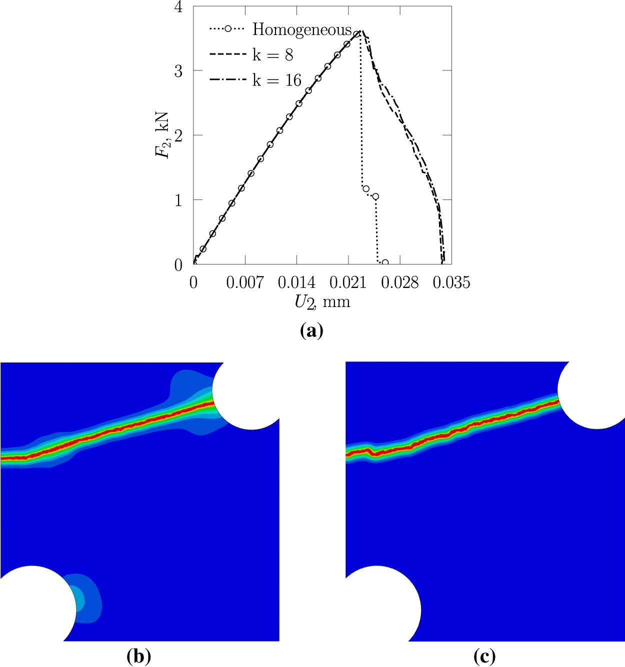
Figure 24: A 2D double-notched specimen (brittle fracture): (a) Force-displacement curves; (b) Crack topology—DNS; (c) Crack topology—k=16.

What was stated about the 2D double-notched specimen in the case of brittle fracture applies to its 3D counterpart. Fig. 25a shows (again) almost identical results of the analysis performed with homogeneous material properties and the fully concurrent procedure for the region before crack initiation and propagation. However, in contrast to a 2D double-notched specimen, a 3D double-notched specimen exhibits a more pronounced loss of material stiffness when analysis is performed using SCA at the microlevel. This can be attributed to the lower value of the inclusion volume fraction, which is approximately twice the value of the inclusion volume fraction in the 2D case. In terms of crack topologies, which are depicted in Fig. 25b,c, the concurrent approach again produces a more irregular crack path than the homogeneous approach, as expected.

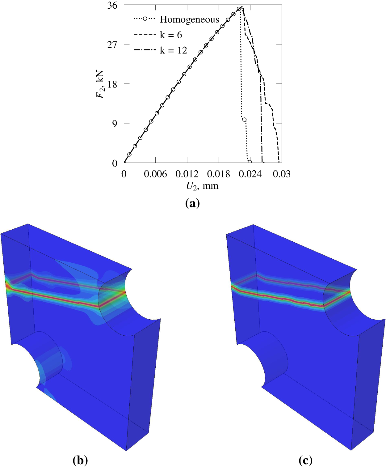
Figure 25: A 3D double-notched specimen (brittle fracture): (a) Force-displacement curves; (b) Crack topology—DNS; (c) Crack topology—k=12.

From Fig. 26a it is clear that the same trend in the force-displacement relationship before the peak force is reached is present once more. However, herein, there is a significant difference between the peak force obtained by DNS and the multiscale concurrent approach. To be more precise, the peak force obtained by DNS analysis sits at a 18.6% higher value. From Fig. 26a it is also visible that the rate of material degradation is noticeably higher in the case of concurrent multiscale analysis. The main factor that influences this behaviour is the value of the macroscopic initial yield strength σ¯y0, which in the case of homogeneous material is determined as the value of homogenised von Mises stress at the homogenised equivalent plastic strain of 0.2%. This means that the homogeneous material enters the elastoplastic region only when von Mises stress exceeds the value of 248.9 MPa, while for the heterogeneous material, that transition will happen at the lower values of the macroscopic von Mises stress. Similarly to brittle fracture, the crack topologies in ductile fracture are again in good agreement—as can be seen from Fig. 26b,c. However, the damaged region obtained by the concurrent multiscale approach (using 16 material clusters) is more localised than that obtained by the DNS (using homogeneous material properties), which is a direct consequence of the presence of material heterogeneity in the analysis.

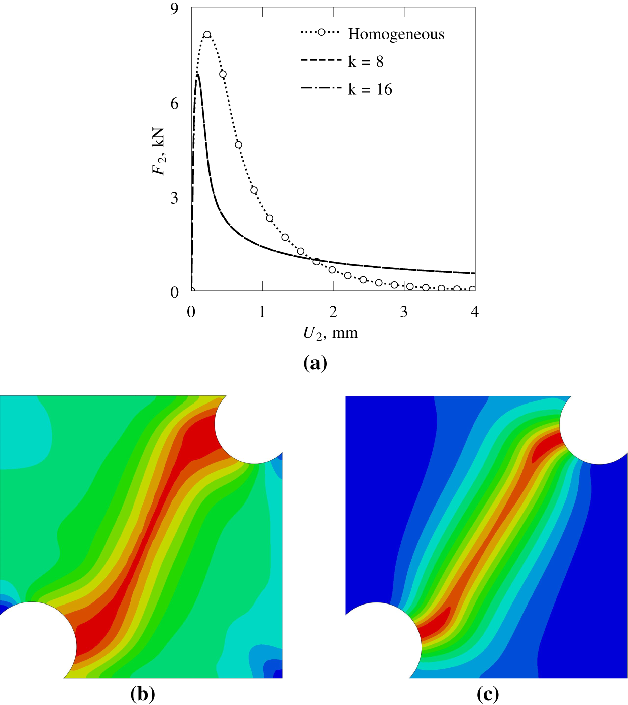
Figure 26: A 2D double-notched specimen (ductile fracture): (a) Force-displacement curves; (b) Crack topology—DNS; (c) Crack topology—k=16.

Analysis of ductile fracture, conducted on the 3D double-notched specimen, shows again that the rate of material degradation after the peak force is reached is higher when the heterogeneous material is modelled using the fully concurrent approach with 6, i.e., 12 material clusters—see Fig. 27a. Although the peak force in the previous example was higher for the DNS (homogeneous material), in this case, the opposite behaviour is observed. However, the concurrent approach gives a value of the peak force that is only 1.1% higher when compared to DNS. The crack phase-field depicted in Fig. 27b,c are in good agreement, with again a more localised damage zone being present when the concurrent multiscale approach is in question. Also, notice that for all the examples shown in the second stage of testing, no difference in the force-displacement relationship is observed between the two different cluster discretisations.

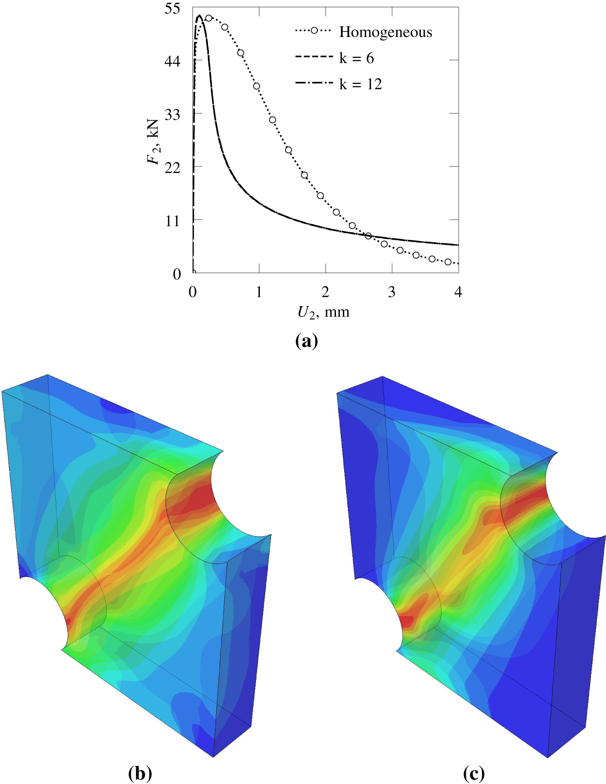
Figure 27: A 2D double-notched specimen (ductile fracture): (a) Force-displacement curves; (b) Crack topology—DNS; (c) Crack topology—k=12.

6  Effect of PF Fracture Parameters on the Fracture Response

Unlike the previous section, where the goal was performance testing and validation of the proposed concurrent framework, this section will focus on the influence of the PF fracture parameters, namely the macroscopic length-scale parameter l¯ and the critical value of energy release rate G¯c. Not only are these parameters important in the process of regularisation of the boundary value problem, which starts to become ill-posed when strain softening occurs, but they also have a direct impact on the overall fracture behaviour. The value of G¯c determines the amount of energy dissipation per unit area in the crack, while the value of l¯ influences the size of a domain on which the diffusion of a discrete crack is taking place. Due to that, it is important to give a better insight on how the value of l¯ as well as G¯c influence the overall fracture response.

Sensitivity analysis includes both brittle and ductile fracture under two- but also three-dimensional configurations, and in total, three different values of l¯ and G¯c are used. Unlike Section 5, where multiple test specimens were subjected to numerical validation, this section will make use of only one test specimen, i.e., the double-notched specimen depicted in Fig. 5c. This sample was used in the previous section in both brittle and ductile fracture simulations, therefore represents a good choice for this task. All calculations are carried out using the developed concurrent framework, and they include decomposition with 8 (for 2D) and 6 (for 3D) material clusters. For the sake of simplicity, 2D unit cell, i.e., 3D unit sphere are the RVEs in question with the MS1 material configuration, which is given by Table 1.

6.1 Influence of the Length-Scale Parameter

As was previously stated, the sensitivity analysis is carried out using three different values of the PF macroscopic parameters. Since the focus of this subsection is to examine the impact of the macroscopic length-scale parameter l¯, its value is subjected to change while the value of the macroscopic critical energy release rate G¯c is held constant.

For the case of brittle fracture in both two- and three-dimensional configurations, the value of G¯c is equal to 3 N/mm, while three different values for l¯ are: 0.2, 0.3 and 0.4 mm. On the other hand, G¯c in the case of ductile fracture is equal to 33 N/mm (an increase by 11 times), while chosen values for l¯ are: 0.4, 0.6 and 0.8 mm. The results showing the influence of the macroscopic length-scale parameter on the fracture response for the case of brittle material are depicted in Fig. 28, while Fig. 29 shows how different values of the macroscopic length-scale parameter influences fracture response in ductile material.

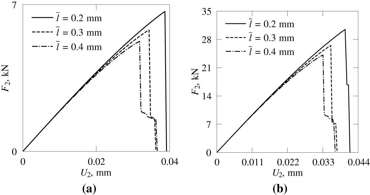
Figure 28: Influence of the value of l¯ on the fracture response: (a) Two-dimensional brittle fracture analysis; (b) Three-dimensional brittle fracture analysis.

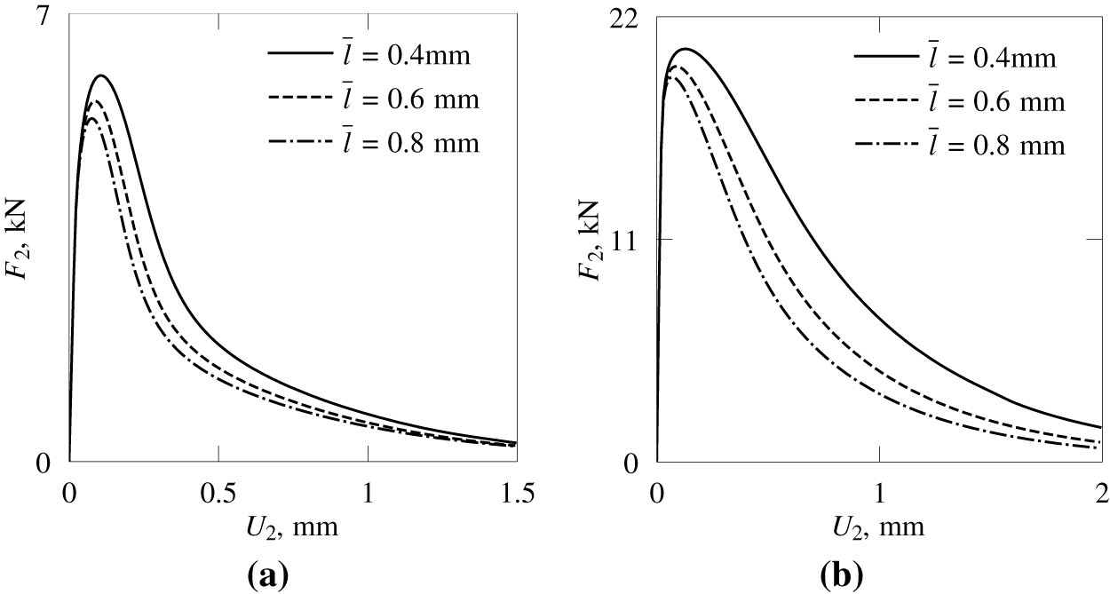
Figure 29: Influence of the value of l¯ on the fracture response: (a) Two-dimensional ductile fracture analysis; (b) Three-dimensional ductile fracture analysis.

From Figs. 28 and 29 it is clear that there is an inverse correlation between the value of the macroscopic length-scale parameter and the value of the peak force. More precisely, with the increase in the value of l¯, the maximum value of the reaction force the sample can reach decreases. The reason for this lies in the fact that when l¯→0, the stress in the crack tip tends to infinity as the discrete crack Γ is recovered. On the other hand, with the increase in l¯, a finite region over which the discrete crack Γ is smeared widens, thus leading to lower values of stress in the region of the crack tip. Lower values of stress ultimately lead to lower values of the peak reaction force, as can be seen from Figs. 28 and 29. After the peak force is reached, all simulations of brittle fracture show an abrupt drop in the overall stiffness, while results for ductile fracture depict a gradual loss of stiffness, which was to be expected.

6.2 Influence of the Critical Value of Energy Release Rate

The procedure for examining the impact of the value of G¯c on the overall fracture response is identical to the procedure conducted for the case of l¯.

For the case of brittle fracture in both two- and three-dimensional configurations, the value of l¯ is equal to 0.3 mm, while three different values for G¯c are: 2, 3 and 4 N/mm. In contrast, ductile fracture analyses exhibit two times larger macroscopic length-scale parameter, i.e., l¯=0.6 mm, while each of the three values of G¯c are multiplied by 11 giving: 22, 33 and 44 N/mm. Results depicting the influence of the value of critical energy release rate are shown by Fig. 30, for the case of brittle fracture, and by Fig. 31, for the case of ductile fracture.

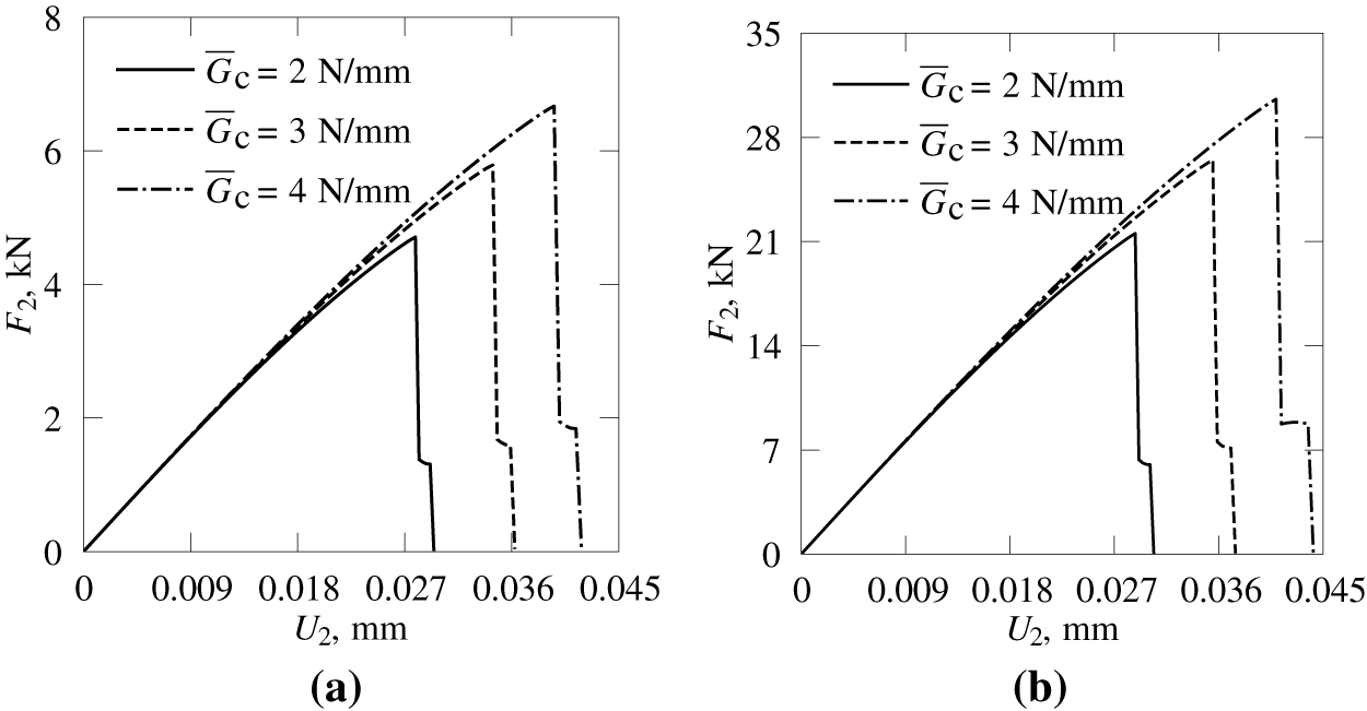
Figure 30: Influence of the value of G¯c on the fracture response: (a) Two-dimensional brittle fracture analysis; (b) Three-dimensional brittle fracture analysis.

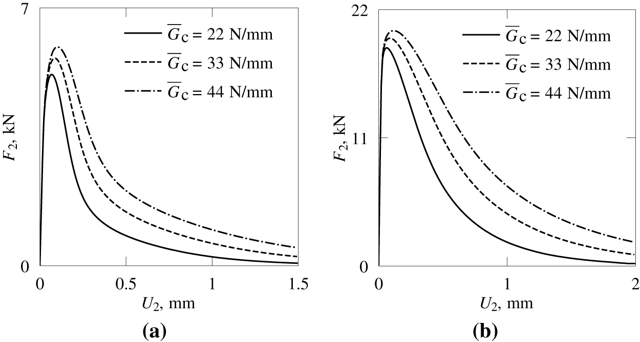
Figure 31: Influence of the value of G¯c on the fracture response: (a) Two-dimensional ductile fracture analysis; (b) Three-dimensional ductile fracture analysis.

Contrary to the previous case where an inverse correlation was present, herein, an increase in the value of G¯c also leads to an increase in the value of the peak reaction force. A higher value of G¯c leads to a higher value of the energy limit that can be dissipated per unit area in the crack. This ultimately results in a need for a higher value of loading necessary to bring about crack initiation and the creation of new surfaces. As expected, different values of G¯c do not impact the post-fracture behaviour, as was the case in the sensitivity analysis of l¯.

7  Conclusion

A novel concurrent multiscale procedure for modelling damage in brittle and ductile heterogeneous materials has been presented. The proposed approach relies on the combination of two methods—self-consistent clustering analysis (SCA) and phase-field (PF) fracture algorithm. The SCA, present at the microlevel, ensures accurate and computationally efficient calculation of the RVE boundary value problem. The efficiency of this ROM results from the drastic reduction of the total number of degrees of freedom at the microlevel, which is achieved by the RVE decomposition into a relatively small number of material clusters k. Being applicable to any constitutive law and any type of microstructure, SCA also enhances the overall flexibility of the proposed concurrent procedure. On the other hand, the PF method at the macrolevel provides an objective and robust calculation of the damage the heterogeneous material has undergone. A non-local continuum damage method, such as PF, does not suffer from the pathological mesh dependence, which ultimately ensures mesh independence and prevents non-physical results at the macrolevel. Similarly to SCA, the PF fracture approach is also applicable to different constitutive laws, thereby enhancing the algorithm’s ability to analyse various types of heterogeneous materials.

A particularly important feature of the proposed concurrent approach is the full decoupling of the damage analysis from the solution of the RVE boundary value problem. This action opens the gate to a more stable and efficient concurrent multiscale analysis, as calculation of damage directly at the microlevel may lead to poor convergence, numerical instability and meaningless results. However, this also removes information on micro crack initiation and propagation, as well as void coalescence since damage analysis is not present at the RVE level. Moreover, the presented procedure requires that both PF fracture parameters (length-scale parameter and the value of critical energy release rate) are known a priori, as they are not obtained from the solution of the RVE boundary problem which is present at each integration point at the macrolevel.

The derived concurrent multiscale procedure is implemented within the Abaqus software architecture using the UMAT subroutine, and tested on several different geometrical specimens that are commonly used in experimental and numerical investigations of damage and fracture. An equal number of analyses were performed for fracture in brittle and ductile heterogeneous materials. The results, which include force-displacement diagrams, crack topologies and CPU times, provide a detailed insight into the computational efficiency, accuracy and robustness of the proposed approach. Also, a separate section is dedicated to the investigation of the influence of PF fracture parameters on the overall fracture response, thus providing a better understanding of the behaviour of the presented framework. Overall, the proposed approach exhibits favourable performance across all evaluated criteria, thereby confirming its effectiveness in modelling of fracture response in heterogeneous materials.

Acknowledgement: Not applicable.

Funding Statement: The authors received no specific funding for this study.

Author Contributions: The authors confirm contribution to the paper as follows: conceptualization, Ante Jurčević, Tomislav Lesičar, Zdenko Tonković and Jurica Sorić; methodology, Ante Jurčević; software, Ante Jurčević; validation, Ante Jurčević, Tomislav Lesičar, Zdenko Tonković and Jurica Sorić; formal analysis, Ante Jurčević; investigation, Ante Jurčević; data curation, Ante Jurčević; writing—original draft preparation, Ante Jurčević; writing—review and editing, Ante Jurčević, Tomislav Lesičar, Zdenko Tonković and Jurica Sorić; supervision, Tomislav Lesičar, Zdenko Tonković and Jurica Sorić. All authors reviewed and approved the final version of the manuscript.

Availability of Data and Materials: The authors confirm that the data supporting the findings of this study are available within the article.

Ethics Approval: Not applicable.

Conflicts of Interest: The authors declare no conflicts of interest.

References

1. Jurčević A. Multiscale modeling of damage in ductile heterogeneous materials [dissertation thesis]. Zagreb, Croatia: Faculty of Mechanical Engineering and Naval Architecture; 2024. [Google Scholar]

2. Galvanetto U, Aliabadi MHF. Multiscale modeling in solid mechanics: computational approaches. London, UK: Imperial College Press; 2010. [Google Scholar]

3. Lesičar T, Tonković Z, Sorić J. A second-order two-scale homogenization procedure using C1 macrolevel discretization. Comput Mech. 2014;54(2):425–41. doi:10.1007/s00466-014-0995-3. [Google Scholar] [CrossRef]

4. Lesičar T, Sorić J, Tonković Z. Large strain, two-scale computational approach using C1 continuity finite element employing a second gradient theory. Comput Methods Appl Mech Eng. 2016;298:303–24. doi:10.1016/j.cma.2015.09.017. [Google Scholar] [CrossRef]

5. Lesičar T, Tonković Z, Sorić J. Two-scale computational approach using strain gradient theory at microlevel. Int J Mech Sci. 2017;126:67–78. doi:10.1016/j.ijmecsci.2017.02.017. [Google Scholar] [CrossRef]

6. De Souza Neto EA, Perić D, Owen DRJ. Computational methods for plasticity: theory and applications. Chichester, UK: Wiley; 2008. [Google Scholar]

7. Gong J, Yuan C, Huang X, Tian W, Li L, Song J. RVE-based finite element analysis of mechanical properties and damage evolution in 2D woven carbon fiber composites. J Mater Res Technol. 2026;41(2021):6074–92. doi:10.1016/j.jmrt.2026.02.128. [Google Scholar] [CrossRef]

8. Sankar HR, Singh H. Representative volume element: existence and extent in cracked heterogeneous medium. Mech Mater. 2023;184(12):104748. doi:10.1016/j.mechmat.2023.104748. [Google Scholar] [CrossRef]

9. El Moumen A, Kanit T, Imad A. Numerical evaluation of the representative volume element for random composites. Eur J Mech A Solids. 2021;86(7):104181. doi:10.1016/j.euromechsol.2020.104181. [Google Scholar] [CrossRef]

10. Bai W, Gong Z, Li Y, Liu J. Determination of the representative volume element model critical size for carbon fiber reinforced polymer composites. Compos Sci Technol. 2023;234:109946. doi:10.1016/j.compscitech.2023.109946. [Google Scholar] [CrossRef]

11. Raju K, Tay T-E, Tan VBC. A review of the FE2 method for composites. Multiscale Multidiscip Model Exp Des. 2021;4(1):1–24. doi:10.1007/s41939-020-00087-x. [Google Scholar] [CrossRef]

12. Zhi J, Poh LH, Tay T-E, Tan VBC. Direct FE2 modeling of heterogeneous materials with a micromorphic computational homogenization framework. Comput Methods Appl Mech Eng. 2022;393(1):114837. doi:10.1016/j.cma.2022.114837. [Google Scholar] [CrossRef]

13. Li M, Magri M, Wang B, Wang B. A novel coupled clustering FFT2 multiscale method for modeling the nonlinear behavior and failure of composites. Comput Methods Appl Mech Eng. 2025;438(6):117854. doi:10.1016/j.cma.2025.117854. [Google Scholar] [CrossRef]

14. Sun W, Fish J, Dhia HB. A variant of the s-version of the finite element method for concurrent multiscale coupling. Int J Multiscale Comput Eng. 2018;16(2):187–207. doi:10.1615/IntJMultCompEng.2018026400. [Google Scholar] [CrossRef]

15. Gierden C, Kochmann J, Waimann J, Svendsen B, Reese S. A review of FE-FFT-based two-scale methods for computational modeling of microstructure evolution and macroscopic material behavior. Arch Comput Methods Eng. 2022;29(6):4115–35. doi:10.1007/s11831-022-09735-6. [Google Scholar] [CrossRef]

16. Schmidt A, Gierden C, Fechte-Heinen R, Reese S, Waimann J. Efficient thermo-mechanically coupled and geometrically nonlinear two-scale FE-FFT-based modeling of elasto-viscoplastic polycrystalline materials. Comput Methods Appl Mech Eng. 2025;435(2):117648. doi:10.1016/j.cma.2024.117648. [Google Scholar] [CrossRef]

17. Liu Z, Fleming M, Liu WK. Microstructural material database for self-consistent clustering analysis of elastoplastic strain softening materials. Comput Methods Appl Mech Eng. 2018;330(41):547–77. doi:10.1016/j.cma.2017.11.005. [Google Scholar] [CrossRef]

18. Putar F, Sorić J, Lesičar T, Tonković Z. A multiscale method for damage analysis of quasi-brittle heterogeneous materials. Comput Model Eng Sci. 2019;120(1):123–56. doi:10.32604/cmes.2019.06562. [Google Scholar] [CrossRef]

19. Sorić J, Lesičar T, Tonković Z. On ductile damage modelling of heterogeneous material using second-order homogenization approach. Comput Model Eng Sci. 2021;126(3):915–34. doi:10.32604/cmes.2021.014142. [Google Scholar] [CrossRef]

20. Lesičar T, Sorić J, Tonković Z. Ductile damage modelling of heterogeneous materials using a two-scale computational approach. Comput Methods Appl Mech Eng. 2019;355:113–34. doi:10.1016/j.cma.2019.06.013. [Google Scholar] [CrossRef]

21. Nguyen VP, Lloberas-Valls O, Stroeven M, Sluys LJ. On the existence of representative volumes for softening quasi-brittle materials—a failure zone averaging scheme. Comput Methods Appl Mech Eng. 2010;199(45–48):3028–38. doi:10.1016/j.cma.2010.06.018. [Google Scholar] [CrossRef]

22. Klawonn A, Lanser M, Mager L, Rege A. Computational homogenization for aerogel-like polydisperse open-porous materials using neural network-based surrogate models on the microscale. Comput Mech. 2026;77(1):297–317. doi:10.1007/s00466-024-02588-9. [Google Scholar] [CrossRef]

23. Kalina KA, Brummund J, Sun W, Kästner M. Neural networks meet anisotropic hyperelasticity: a framework based on generalized structure tensors and isotropic tensor functions. Comput Methods Appl Mech Eng. 2025;437(1):117725. doi:10.1016/j.cma.2024.117725. [Google Scholar] [CrossRef]

24. Feng N, Zhang G, Khandelwal K. Finite strain FE2 analysis with data-driven homogenization using deep neural networks. Comput Struct. 2022;263(3):106742. doi:10.1016/j.compstruc.2022.106742. [Google Scholar] [CrossRef]

25. Wu L, Nguyen VD, Kilingar NG, Noels L. A recurrent neural network-accelerated multi-scale model for elasto-plastic heterogeneous materials subjected to random cyclic and non-proportional loading paths. Comput Methods Appl Mech Eng. 2020;369(2):113234. doi:10.1016/j.cma.2020.113234. [Google Scholar] [CrossRef]

26. Jones RE, Templeton JA, Sanders CM, Ostien JT. Machine learning models of plastic flow based on representation theory. Comput Model Eng Sci. 2018;117(3):309–42. doi:10.31614/cmes.2018.04285. [Google Scholar] [CrossRef]

27. Qu T, Di S, Feng YT, Wang M, Zhao T, Wang M. Deep learning predicts stress–strain relations of granular materials based on triaxial testing data. Comput Model Eng Sci. 2021;128(1):129–44. doi:10.32604/cmes.2021.016172. [Google Scholar] [CrossRef]

28. Deng S, Shirin H, Wang L, Apelian D, Bostanabad R. Data-driven physics-constrained recurrent neural networks for multiscale damage modeling of metallic alloys with process-induced porosity. Comput Mech. 2024;74(1):191–221. doi:10.1007/s00466-023-02429-1. [Google Scholar] [CrossRef]

29. Hu W, Cheng H, Zhang K, Li Y, Yang H, Li Y, et al. A novel concurrent multiscale damage analysis method enhanced by physics-informed neural network for composite joint. Compos Sci Technol. 2026;275(28):111483. doi:10.1016/j.compscitech.2025.111483. [Google Scholar] [CrossRef]

30. Dvorak GJ. Transformation field analysis of inelastic composite materials. Proc R Soc A. 1992;437(1900):311–27. doi:10.1098/rspa.1992.0063. [Google Scholar] [CrossRef]

31. Michel JC, Suquet P. Nonuniform transformation field analysis. Int J Solids Struct. 2003;40(25):6937–55. doi:10.1016/S0020-7683(03)00346-9. [Google Scholar] [CrossRef]

32. Yvonnet J, He Q-C. The reduced model multiscale method (R3M) for the non-linear homogenization of hyperelastic media at finite strains. J Comput Phys. 2007;223(1):341–68. doi:10.1016/j.jcp.2006.09.019. [Google Scholar] [CrossRef]

33. Liu Z, Bessa MA, Liu WK. Self-consistent clustering analysis: an efficient multi-scale scheme for inelastic heterogeneous materials. Comput Methods Appl Mech Eng. 2016;306(1):319–41. doi:10.1016/j.cma.2016.04.004. [Google Scholar] [CrossRef]

34. Liu Z. Reduced-order homogenization of heterogeneous material systems: from viscoelasticity to nonlinear elasto-plastic softening material [dissertation thesis]. Evanston, IL, USA: Northwestern University; 2016. [Google Scholar]

35. Lippmann BA, Schwinger J. Variational principles for scattering processes I. Phys Rev. 1950;79(3):469–80. doi:10.1103/PhysRev.79.469. [Google Scholar] [CrossRef]

36. Tang S, Zhang L, Liu WK. From virtual clustering analysis to self-consistent clustering analysis: a mathematical study. Comput Mech. 2018;62(6):1443–60. doi:10.1007/s00466-018-1573-x. [Google Scholar] [CrossRef]

37. Yu C, Kafka OL, Liu WK. Self-consistent clustering analysis for multiscale modeling at finite strains. Comput Methods Appl Mech Eng. 2019;349(5330):339–59. doi:10.1016/j.cma.2019.02.027. [Google Scholar] [CrossRef]

38. Ferreira BP, Cardoso Coelho RP, Andrade Pires FM, Bessa MA. Finite strain self-consistent clustering analysis under multiplicative kinematics. Comput Struct. 2025;316:107886. doi:10.1016/j.compstruc.2025.107886. [Google Scholar] [CrossRef]

39. Zhang L, Tang S, Yu C, Zhu X, Liu WK. Fast calculation of interaction tensors in clustering-based homogenization. Comput Mech. 2019;64(2):351–64. doi:10.1007/s00466-019-01719-x. [Google Scholar] [CrossRef]

40. He C, Gao J, Li H, Ge J, Chen Y, Liu J, et al. A data-driven self-consistent clustering analysis for the progressive damage behavior of 3D braided composites. Compos Struct. 2020;249:112471. doi:10.1016/j.compstruct.2020.112471. [Google Scholar] [CrossRef]

41. Liu T-R, Yang Y, Bacarreza OR, Tang S, Aliabadi MH. An extended full field self-consistent cluster analysis framework for woven composite. Int J Solids Struct. 2023;281(6):112407. doi:10.1016/j.ijsolstr.2023.112407. [Google Scholar] [CrossRef]

42. Han X, Gao J, Fleming M, Xu C, Xie W, Meng S, et al. Efficient multiscale modeling for woven composites based on self-consistent clustering analysis. Comput Methods Appl Mech Eng. 2020;364:112929. doi:10.1016/j.cma.2020.112929. [Google Scholar] [CrossRef]

43. Nie Y, Li Z, Cheng G. Efficient prediction of the effective nonlinear properties of porous material by FEM-cluster based analysis (FCA). Comput Methods Appl Mech Eng. 2021;383(3):113921. doi:10.1016/j.cma.2021.113921. [Google Scholar] [CrossRef]

44. Wu S, Guo L, Li Z, Zheng T, Huang J, Han X, et al. A highly efficient self-consistent clustering analysis method with field refinement capability for the mesoscale damage behavior of 3D woven composites. Compos Sci Technol. 2024;252(12):110609. doi:10.1016/j.compscitech.2024.110609. [Google Scholar] [CrossRef]

45. Wu S, Guo L, Li Z, Ding J, Zhuo Y. A damage-related adaptive self-consistent clustering analysis method with localized refinement capability for the damage problem of 3D woven composites. Compos Sci Technol. 2024;257(10):110814. doi:10.1016/j.compscitech.2024.110814. [Google Scholar] [CrossRef]

46. Li M, Li H, Wang B, Wang B. Self-consistent clustering analysis for homogenisation of heterogeneous plates. Int J Numer Methods Eng. 2026;127(2):e70231. doi:10.1002/nme.70231. [Google Scholar] [CrossRef]

47. Vu G, Diewald F, Timothy JJ, Gehlen C, Meschke G. Reduced order multiscale simulation of diffuse damage in concrete. Materials. 2021;14(14):3830. doi:10.3390/ma14143830. [Google Scholar] [CrossRef]

48. Ferreira BP, Andrade Pires FM, Bessa MA. Adaptivity for clustering-based reduced-order modeling of localized history-dependent phenomena. Comput Methods Appl Mech Eng. 2022;393(1):114726. doi:10.1016/j.cma.2022.114726. [Google Scholar] [CrossRef]

49. Iskhakov T, Timothy JJ, Meschke G. Expansion and deterioration of concrete due to ASR: micromechanical modeling and analysis. Cem Concr Res. 2019;115(3):507–18. doi:10.1016/j.cemconres.2018.08.001. [Google Scholar] [CrossRef]

50. Miehe C, Welschinger F, Hofacker M. Thermodynamically consistent phase-field models of fracture: variational principles and multi-field FE implementations. Int J Numer Methods Eng. 2010;83(10):1273–311. doi:10.1002/nme.2861. [Google Scholar] [CrossRef]

51. Seleš K, Lesičar T, Tonković Z, Sorić J. A residual control staggered solution scheme for the phase-field modeling of brittle fracture. Eng Fract Mech. 2019;205(582–593):370–86. doi:10.1016/j.engfracmech.2018.09.027. [Google Scholar] [CrossRef]

52. Lesičar T, Polančec T, Tonković Z. Convergence check phase-field scheme for modelling of brittle and ductile fractures. Appl Sci. 2023;13(13):7776. doi:10.3390/app13137776. [Google Scholar] [CrossRef]

53. Ambati M, Kruse R, De Lorenzis L. A phase-field model for ductile fracture at finite strains and its experimental verification. Comput Mech. 2016;57(1):149–67. doi:10.1007/s00466-015-1225-3. [Google Scholar] [CrossRef]

54. Miehe C, Aldakheel F, Raina A. Phase field modeling of ductile fracture at finite strains: a variational gradient-extended plasticity-damage theory. Int J Plast. 2016;84:1–32. doi:10.1016/j.ijplas.2016.04.011. [Google Scholar] [CrossRef]

55. Ambati M, Gerasimov T, De Lorenzis L. A review on phase-field models of brittle fracture and a new fast hybrid formulation. Comput Mech. 2014;55(2):383–405. doi:10.1007/s00466-014-1109-y. [Google Scholar] [CrossRef]

56. Liu G, Li Q, Msekh MA, Zuo Z. Abaqus implementation of monolithic and staggered schemes for quasi-static and dynamic fracture phase-field model. Comput Mater Sci. 2016;121(4):35–47. doi:10.1016/j.commatsci.2016.04.009. [Google Scholar] [CrossRef]

57. Borden MJ, Verhoosel CV, Scott MA, Hughes TJR, Landis CM. A phase-field description of dynamic brittle fracture. Comput Methods Appl Mech Eng. 2012;217–220(8):77–95. doi:10.1016/j.cma.2012.01.008. [Google Scholar] [CrossRef]

58. Seleš K, Aldakheel F, Tonković Z, Sorić J, Wriggers P. A general phase-field model for fatigue failure in brittle and ductile solids. Comput Mech. 2021;67(5):1431–52. doi:10.1007/s00466-021-01996-5. [Google Scholar] [CrossRef]

59. Seleš K, Jurčević A, Tonković Z, Sorić J. Crack propagation prediction in heterogeneous microstructure using an efficient phase-field algorithm. Theor Appl Fract Mech. 2019;100(11):289–97. doi:10.1016/j.tafmec.2019.01.022. [Google Scholar] [CrossRef]

60. Zheng S, Huang R, Lin R, Liu Z. A phase field solution for modelling hyperelastic material and hydrogel fracture in ABAQUS. Eng Fract Mech. 2022;276(7414):108894. doi:10.1016/j.engfracmech.2022.108894. [Google Scholar] [CrossRef]

61. Arash B, Zakavati S, Bahtiri B, Jux M, Rolfes R. Phase-field modeling of fracture in viscoelastic–viscoplastic thermoset nanocomposites under cyclic and monolithic loading. Eng Comput. 2025;41(1):681–701. doi:10.1007/s00366-024-02041-8. [Google Scholar] [CrossRef]

62. Li P, Li W, Li B, Yang S, Shen Y, Wang Q, et al. A review on phase field models for fracture and fatigue. Eng Fract Mech. 2023;289:109419. doi:10.1016/j.engfracmech.2023.109419. [Google Scholar] [CrossRef]

63. MacQueen J. Some methods for classification and analysis of multivariate observations. In: Proceedings of the Fifth Berkeley Symposium on Mathematical Statistics and Probability; 1967 Jul 18–21; Berkeley, CA, USA. p. 281–98. [Google Scholar]

64. Kohonen T. The self-organizing map. Neurocomputing. 1998;21(1–3):1–6. doi:10.1016/S0925-2312(98)00030-7. [Google Scholar] [CrossRef]

65. Li H, Kafka OL, Gao J, Yu C, Nie Y, Zhang L, et al. Clustering discretization methods for generation of material performance databases in machine learning and design optimization. Comput Mech. 2019;64(2):281–305. doi:10.1007/s00466-019-01716-0. [Google Scholar] [CrossRef]

66. Francfort GA, Marigo J-J. Revisiting brittle fracture as an energy minimization problem. J Mech Phys Solids. 1998;46(8):1319–42. doi:10.1016/S0022-5096(98)00034-9. [Google Scholar] [CrossRef]

67. Griffith AA VI. The phenomena of rupture and flow in solids. Philos Trans A Math Phys Eng Sci. 1921;221(582–593):163–98. doi:10.1098/rsta.1921.0006. [Google Scholar] [CrossRef]

68. Kuhn C, Schlüter A, Müller R. On degradation functions in phase field fracture models. Comput Mater Sci. 2015;108(4):374–84. doi:10.1016/j.commatsci.2015.05.034. [Google Scholar] [CrossRef]

69. Amor H, Marigo J-J, Maurini C. Regularized formulation of the variational brittle fracture with unilateral contact: numerical experiments. J Mech Phys Solids. 2009;57(8):1209–29. doi:10.1016/j.jmps.2009.04.011. [Google Scholar] [CrossRef]

70. Freddi F, Royer-Carfagni G. Regularized variational theories of fracture: a unified approach. J Mech Phys Solids. 2010;58(8):1154–74. doi:10.1016/j.jmps.2010.02.010. [Google Scholar] [CrossRef]

71. Wu J-Y, Nguyen WP, Zhou H, Huang Y. A variationally consistent phase-field anisotropic damage model for fracture. Comput Methods Appl Mech Eng. 2020;358(8):112629. doi:10.1016/j.cma.2019.112629. [Google Scholar] [CrossRef]

72. Nagaraja S, Carrara P, De Lorenzis L. Experimental characterization and phase-field modeling of anisotropic brittle fracture in silicon. Eng Fract Mech. 2023;293(2):109684. doi:10.1016/j.engfracmech.2023.109684. [Google Scholar] [CrossRef]

73. Clayton JD. Computational modeling of dual-phase ceramics with finsler-geometric phase field mechanics. Comput Model Eng Sci. 2019;120(2):333–50. doi:10.32604/cmes.2019.06342. [Google Scholar] [CrossRef]

74. Ruan H, Peng X-L, Yang Y, Gross D, Xu B-X. Phase-field ductile fracture simulations of thermal cracking in additive manufacturing. J Mech Phys Solids. 2024;191(5):105756. doi:10.1016/j.jmps.2024.105756. [Google Scholar] [CrossRef]

75. Alessi R, Ambati M, Gerasimov T, Vidoli S, De Lorenzis L. Comparison of phase-field models of fracture coupled with plasticity. In: Oñate E, Peric D, de Souza Neto E, Chiumenti M, editors. Advances in computational plasticity: a book in honour of D. Roger J. Owen. Berlin/Heidelberg, Germany: Springer; 2018. p. 1–21. [Google Scholar]

76. Tojega V, Kulachenko A, Östlund S, Gasser TC. Hybrid of monolithic and staggered solution techniques for the computational analysis of fracture, assessed on fibrous network mechanics. Comput Mech. 2023;71(1):39–54. doi:10.1007/s00466-022-02197-4. [Google Scholar] [CrossRef]

77. Li P, Lv G, Li W, Fan H, Wang Q, Zhou K. Fully coupled electro-chemo-thermo-mechanical phase-field fracture modeling for solid-state batteries. Int J Solids Struct. 2026;328(47):113831. doi:10.1016/j.ijsolstr.2026.113831. [Google Scholar] [CrossRef]

78. Gerasimov T, De Lorenzis L. A line search assisted monolithic approach for phase-field computing of brittle fracture. Comput Methods Appl Mech Eng. 2016;312(37):276–303. doi:10.1016/j.cma.2015.12.017. [Google Scholar] [CrossRef]

79. Kristensen PK, Martínez-Pañeda E. Phase field fracture modelling using quasi-Newton methods and a new adaptive step scheme. Theor Appl Fract Mech. 2020;107(8):102446. doi:10.1016/j.tafmec.2019.102446. [Google Scholar] [CrossRef]

80. Matlab documentation. [cited 2026 Jan 1]. Available from: https://www.mathworks.com/help/matlab/index.html. [Google Scholar]

81. Simulia abaqus 2016 user subroutines reference guide. [cited 2026 Jan 1]. Available from: http://130.149.89.49:2080/v2016/books/sub/default.htm?startat=ami01.html. [Google Scholar]

82. Čanžar P, Tonković Z, Kodvanj J. Microstructure influence on fatigue behaviour of nodular cast iron. Mater Sci Eng A. 2012;556:88–99. doi:10.1016/j.msea.2012.06.062. [Google Scholar] [CrossRef]

83. Cost JR, Janowski KR, Rossi RC. Elastic properties of isotropic graphite. Philos Mag. 1968;17(148):851–4. doi:10.1080/14786436808223035. [Google Scholar] [CrossRef]

84. MatWeb. [cited 2026 Jan 1]. Available from: https://www.matweb.com. [Google Scholar]