Filter and Embedded Feature Selection Methods to Meet Big Data Visualization Challenges

1  Introduction

The challenge of visualizing a big data collection is difficult. Traditional data presentation methods have hit a few stumbling blocks as data continues to rise exponentially. Users should be able to spot missing, incorrect, or duplicate information using visualization tools and approaches. Represented the big data visualization challenges in (1) Perceptual scalability; (2) Real-time scalability; and (3) Interactive scalability. There are several opportunities to address the challenges above, including (1) Data reduction methods based on sampling, filtering, and embedded; (2) Reducing latency based on pre-computed data, parallelize data processing and rendering, and apredictive middleware [1,2]. This paper used the opportunity of data reduction based on feature selection methods to see their impact before analyzing and visualizing the data. The dimensionality of data is expanding across many fields and applications, and feature selection has become essential in big data mining [3,4]. Thus, machine learning techniques such as classification algorithms face the “curse of dimensionality” when dealing with big datasets because of the large numbers of features or dimensions, where small and informative features subsets are selected utilizing the features selection method. As a result of the high dimensionality of the data, traditional machine learning fails to perform well on vast volumes of data [5]. Feature selection (FS) is a set of steps that are used to decide which relevant features/attributes to include in predictive modeling and which irrelevant features to leave out. It is a very important task that helps machine learning classifiers reduce error rates, computation time, overfitting, and improve the accuracy of their classifications. It has shown that it works in many different areas [6]. It is a preprocessing approach used to identify the essential characteristics of a particular situation. It has traditionally been used to solve many issues [7]. It is a method of global optimization in machine learning [8]. However, feature selection has been a hot topic for decades, and improves the efficiency of data mining and analysis [9]. One of the most challenging tasks is the selection of relevant features from the initial set of available features. The selection should be to maximize the improvement in learning performance over the performance of the original feature set [10], as the feature selection reduces the dimensionality of feature space. So far, several strategies for feature selection have been presented [11]. Moreover, multiple feature selection frameworks have been established over time. An examination of their accomplishments and shortcomings may be necessary to appreciate their strengths and weaknesses [12]. It’s also a crucial step in data mining and pattern recognition difficulties. Thus, it removes unrepresentative traits or picks a subset of a training dataset to improve performance. Some of the benefits of performing feature selection are as follows:

•   To reduce the impact of the dimensionality curse.

•   Avoiding problems caused by overfitting.

•   It reduces the amount of time it takes to train a model.

•   It is improving the generalization capabilities of models that have been developed.

Generalized feature selection methods may be categorized as filters, wrappers, embedded and hybrid approaches. Filters are the most common type of feature selection method [13]. Because the primary goal of the features selection technique is to reduce data volume, speed up training time and increase the accuracy of model classification, this is effective in the processes of analyzing, mining, and visualizing big data to meet its challenges. The goal of data analytics is to find patterns in data. However, in the era of big data, the task is even more difficult [11]. Before big data visualization, the data must be prepared, cleaned, missing values processed, and extracted the best features affecting the goal to obtain a reliable visualization to get the best short data set from the original data and help the decision-maker to make the right decision. Thus, the paper faced the challenges of visualizing big data by using features selection methods to reduce the features of big data, obtain the best subset of features affecting the goal, and be analyzed and visualized to know the patterns within the data. The paper used two feature selection methods, the filter method by using (SP) method with embedded method by using (RFI) algorithm and compared them to see which one to use before visualizing the data. Then has been used two classification algorithms to measure the accuracy of the data before and after the preprocessing and feature selection process of the data based on eight datasets from different domains with high and small dimensions. The main motive of the study is to find a method that facilitates the visualization of the large volume of data and the treatment of its problems, where we have contributed to reducing big data and getting rid of redundant data and data that does not influence decision-making before the visualization to addressing big data visualization Challenges by the use of data reduction methods based feature selection. Work was performed using Python on a computer with specification Intel(R) Core(TM) i3-2350M CPU @ 2.30 GHz, with (RAM): 4.00 GB, with 64-bit Operating System, and with Windows 10. This paper is arranged as follows: Section 2 briefly describes the related works. Section 3 describes the methods used in this study. Section 4 represents the research methodology used in this study. The results obtained will be explained in Section 5. Finally, Section 6 will be presents the conclusions and future work of this study.

2  Related Works

The authors in [2] suggested the use of some modern visual analytics platforms to overcome the challenges of big data visualization. The results showed that these platforms could handle most of the problems people face in general. But there are still problems that need more work, such as uncertainty and cognitive bottlenecks in people. In [14], the authors explain the problems related to big data visualization and mention that current developments to meet the challenges focus on creating tools that enable the end-user to achieve good and fast results when dealing with big data. But they note that some problems with large data visualization, like how people see large images, information loss, the need for high performance, and fast image changes, are still not solved and will be studied in the future. In [15], the authors discussed and studied big data and its visualization, visualization tools and techniques. Data visualization is an important part of research because the amount of data is growing so quickly. All organizations can’t buy the domains that are important for data analysis because they don’t have enough money or the right infrastructure. So, advanced tools and technologies are needed to analyze big data, so open source data visualization tools are used. The authors in [16], used ten chaotic maps to make the interior search algorithm (ISA) algorithms converge faster and be more accurate. The proposed chaotic interior search algorithm (CISA) is tested on a diverse subset of 13 benchmark functions that have both unimodal and multimodal properties. The simulation results show that chaotic maps, especially the tent map, can improve the performance of ISA by a lot. But some challenges still remain. In [17], the authors gave a detailed look at meta-heuristic techniques that are based on nature and how they are used in the feature selection process. For the researcher who prefers to design or analyze the performance of divergent meta-heuristic techniques in solving feature selection problems, research gaps have been identified. The authors in [18], used five new meta-heuristic techniques based on swarm intelligence. Chaotic variants of satin-bird optimization (SBO) were used to choose features, and their results were compared. Here, five different kinds of SBO were made by combining the features of SBO with those of four different chaotic maps: the circle map, the chebyshev map, the sinusoidal map, the tent map, and the gauss map. From the experiments, it was seen that the SBO algorithm was more accurate and better at predicting cardiac arrhythmia than the bGWO, DA, BOA, and ALO algorithms. Also, BOA and ALO seem to work best when the focus is only on size dimensions. In [19], the authors used seven different Swarm Intelligence (SI)-based metaheuristic techniques, such as Ant Lion Optimizer (ALO), Gray Wolf Optimization (GWO), Dragonfly Algorithm (DA), Satin Bowerbird Optimization (SBO), Harris Hawks Optimization (HHO), Butterfly Optimization Algorithm (BOA), Whale Optimization Algorithm (WOA), and one hybrid SI-based approach (WOA and Simulated Annealing (SA)) to find an optimal set of features for bi-objective stress diagnosis problem. Other (SI)-based feature selection metaheuristic strategies, such as (ALO), (BOA), (GWO), (DA), (SBO), (HHO), and (WOA) itself, were shown to be less exact and successful than the hybrid approach of (WOA) and (SA). By selecting the most competent region pointed out by (WOA), the usage of (SA) in (WOA-SA) improved the exploitation phase. When only a small number of characteristics are required, however, (BOA’s) performance is found to be good. In [20], the authors looked at the main ideas of FS and how they have been used recently in big data bioinformatics. Instead of the usual filter, wrapper, and embedded FS approaches, they look at FS as a combinatorial (discrete) optimization problem and divided FS methods into exhaustive search, heuristic search, and hybrid methods. Heuristic search methods can be further divided into those with or without data-distilled feature ranking. In [1], the authors Identify challenges and opportunities for big data visualization with a review of some current visualization methods and tools. These methods and tools could help us see big data in new ways. In [21], the authors suggested several commonly-used assessment metrics for feature selection. They covered a variety of approaches to feature selection that are supervised, unsupervised, and semi-supervised, which are extensively employed in machine learning issues like classification and clustering, some challenges still remain. In [22], the authors proposed a high-performance solar radiation recognition model to deal with nonlinear dynamics in time series. We used random forest (RF) and a features selection strategy, with the help of the moving average indicator, 45 features were taken from the data on temperature, pressure, wind speed, humidity, and solar radiation. Also, a total of 50 features have been taken out, along with the five features that were taken out based on the values of the five parameters that were set before. The forward selection method was used to find the features that will improve model performance. In [23], the authors suggested that a bagging-based ensemble strategy improves feature selection stability in medical datasets by lowering data variance, they experimented with four microarray datasets, each of which had a small number of samples and a high number of dimensions. They used five well-known feature selection algorithms on each dataset to pick a different number of features. The proposed method shows a big improvement in the stability of selection while at least keeping the classification accuracy. In every case, the improvement in stability is between 20% and 50%. This means that the chances of picking the same features went up by 20 to 50 percent. This is usually accompanied by a rise in classification accuracy, which shows that the stated results are stable. In [24], the authors compare and contrast the performance of state-of-the-art feature selection algorithms on large, high-dimensional data collections, and the goal of the analyses is to look at how different filter methods work, compare how fast they run and how well they predict, and give advice on how to use them. Based on 16 high-dimensional classification data sets, 22 filter methods are looked at in terms of how long they take to run and how well they work when combined with a classification method. It is concluded that there is no group of filter methods that always works better than all the others. However, suggestions are made for filter methods that work well on many of the data sets. Also, groups of filters that rank the features in the same order are found. In [25], the authors proposed a comparative study to analyze and classify the different selection methods. When a broad classification of these approaches is conducted, state-of-the-art swarm intelligence-based feature selection methods are explored, and the merits and shortcomings of the various swarm intelligence-based feature selection methods are reviewed. In [13], the authors look at how well different types of feature selection algorithms work together with ensemble feature selection strategies to improve classification performance. The union, intersection, and multi-intersection procedures are among the approaches for merging multiple feature selection results. In [26], the authors presented a new hybrid filter/aggregator algorithm for feature selection (LMFS). This algorithm is effective and efficient; it was found that the distance-based classes (LSSVM and k-NN) were more suitable for selecting the final subsets in LMFS from other classifiers. In [27], the authors developed a Hybrid Genetic Algorithm with Embedded Wrapper (HGAWE) for selecting features in building a learning model and classifying cancer, the (HGAWE) methodology beats the current combined approaches in terms of feature selection and classification accuracy, according to an empirical research using simulation data and five gene microarray data sets. In [28], the authors proposed a new way to choose features when training examples are only partially labelled in a multi-class classification setting. It is based on a new modification of the genetic algorithm that creates and evaluates candidate feature subsets during an evolutionary process, taking feature weights into account and recursively getting rid of irrelevant features. Several state-of-the-art semi-supervised feature selection approaches have been tested against different data sets to see how well our method works. In [29], the authors proposed a greedy search method for selecting the features subset that would maximize classification results, and the results of tests, which used standard databases of handwritten words from the real world, showed that the idea works. A summary of this part. In recent research, different techniques, algorithms, and methods were used to pick features to reduce the amount of data and get the best-selected subset from the original set of data. This is one of the positives about the related works. But none of this recent writing has the function of feature selection to deal with the challenges and problems of big data visualization that decision-makers face. So, big data visualization still has some problems and needs a lot of work to fix them. This is one of the negatives about the related works. Thus, this paper proposes data reduction based on feature selection methods to reduce data volume to meet the problems and challenges of big data visualization. It give good results, which were presented later.

3  Methods

3.1 Features Selection

Features selection is an important topic in machine learning since it has a big impact on model performance. Extraneous attributes are removed from models to increase efficiency, make them easier to understand and reduce runtime. There are three (3) types of feature selection: embedded, wrapper, and filter [30]. For more clarification, see Fig. 1.

Figure 1: Illustrative example of feature selection

3.1.1 Filter Method

The filter method is a data preparation approach that is extensively utilized. This strategy combines ranking techniques with the main criteria and selects sorting systems. Before beginning the classification process, the ranking procedure removes irrelevant features. The benefits of this method are its simplicity, spectacular outcomes, relevant features, and independence from any machine learning algorithm [30]. Multivariate statistical approaches are used to evaluate the rank of the complete feature subset in this category, which is based on the Subset Evaluation. Multivariate statistical techniques take into account feature dependency, eliminating the requirement for a classifier; in terms of computing complexity, it is also more efficient than wrapper approaches [31]. The filter algorithms evaluate the characteristics’ relevancy. A ranking criterion is used to assess feature significance, and features that score below a certain threshold are deleted. Information gain, stepwise regression, and PCA are filter-based feature selection methods. This method is quick and does not require classification algorithms [13]. For example, “SP” (Choose characteristics based on a percentage of the best results). One of the simplest criteria is the pearson correlation coefficient [32] defined as:

R(i)=covv(xi,Y)var(xi)*var(Y)(1)

where xi is the ith variable, Y is the output (class labels), cov () is the covariance and var () the variance. Correlation ranking can only detect linear dependencies between variable and target.

Information theoretic ranking criteria [32] use the measure of dependency between two variables. To describe mutual Information (MI) we must start with Shannons definition for entropy given by:

H(Y)=−∑yp(y)log⁡(p(y))(2)

Eq. (2) [32] represents the uncertainty (information content) in output Y. Suppose we observe a variable X then the conditional entropy is given by:

H(Y∣X)=−∑∑p(x,y)log⁡(p(y∣x))(3)

Eq. (3) [32] implies that by observing a variable X, the uncertainty in the output Y is reduced. The decrease in uncertainty is given as:

I(Y,X)=H(Y)−H(Y∣X)(4)

This gives the MI between Y and X, if X and Y are independent then MI will be zero and greater than zero if they are dependent. This implies that one variable can provide information about the other thus proving dependency. The definitions provided above are given for discrete variables and the same can be obtained for continuous variables by replacing the summations with integrations [32]. The MI can also be defined as a distance measure given by:

K(f,g)=∫f(y)log⁡(f(y)g(y))(5)

The measure K in Eq. (5) is the Kullback–Leibler divergence [32] between two densities which can also be used as a measure of MI. From the above equations.

3.1.2 Wrapper Method

The wrapped method looks for features that fit each machine learning algorithm. Until an adequate feature is found, the wrapped strategy is used before and after the machine learning process. Prediction accuracy and goodness of fit compare classification and grouping features [30]. The predictor’s performance represents an objective function that is used to evaluate the representativeness of the feature subset; unlike filter techniques, where during the search technique, many feature subsets are constructed and examined to evaluate a feature subset, the predictor is trained and tested. Wrapper techniques allow for interaction between features subset searches and predictor selection and consideration of feature dependencies. These include genetic algorithms (GA) and particle swarm optimization (PSO). Wrapper techniques are often computationally expensive because the predictor must be trained and tested [13]. This technique uses a supervised learning algorithm integrated into the process when selecting features. It assigns a value to each feature based on the subset evaluation technique. The correlations and dependencies between them are considered [31]. Multi-objective genetic algorithm is used to solve the big data view selection problem as a bi-objective optimization problem [33]. The improved particle swarm optimization is set up to make it easier to evaluate the credibility of big data found on the web [34].

3.1.3 Embedded Method

Embedded methods keep track of each step of the model training process and look for features that help for specific steps. The regularisation method is a way to give a value to features that aren’t good enough by setting a threshold, e.g., the LASSO algorithm, the Elastic Net algorithm, and the Random Forest Importance (RFI) algorithm [30]. Embedded techniques look for an appropriate feature subset as part of the classifier design, reducing the time to reclassify different subsets in wrapper techniques. The search for features subsets is part of the classifier training process. The SVM, ANN, RFC, and DT techniques are well-known embedded feature selection classifiers [13]. During the development of a classifier, the optimal feature subset is sought. The method for determining the appropriate feature subset varies depending on the classification algorithm in use. The embedded technique has the same benefits as the wrapper strategy, but it is superior to the wrapper strategy in terms of computational complexity, which is a considerable benefit [31]. In this study, we focused on using the “SP” method, which is one of the Filter techniques, and we also used a modern method “(RFI)”. It is one of the methods of embedded techniques. The objective function is set up in such a way that selecting a feature maximizes the MI between the feature and the class output while minimizing the MI between the selected feature and the subset of previously selected features. This is written as the following equation as equation [32].

I(Y,f)−β∑s∈SI(f;s)(6)

where Y is the output, f is the currently selected feature, s is a feature in the already selected subset S, and b determines the relevance of the MI between the current feature f and the subset S features. A Neural Network classifier is used to classify the output subset. Because the inter-feature MI is employed in the calculation to choose the non-redundant features, Eq. (6) will select a better subset [32].

The mRMR (max-relevancy, min-redundancy) [32] is another method based on MI. It uses similar criteria as in Eq. (7) given as:

I(xj;C)−1m−1∑xl∈Sm−1I(xj;xl)(7)

where xi is the math feature in subset S and set Sm−1 is the subset with m 1 features that has been chosen so far. A two-stage technique is used instead of a greedy algorithm [32].

3.1.4 Hybrid Method

The hybrid approach is made so that both the filter and wrapper approaches can be used. So, it has both the high performance of the wrapper approach and the efficiency of the filter approach [35]. It is made up of two steps. The first step is to reduce the size of the feature space. Next, the wrapper method is used to choose the best subset of features. The hybrid model, on the other hand, may be less accurate because the filter and the wrapper are done in separate steps [36]. The ensemble approach is based on the idea that the work of a group of experts is better than the work of a single expert [37]. A single wrapper approach could easily do well in one dataset but badly in another. So, combining more than one method leads to an overall lower error rate [36].

3.2 Classification Algorithms

Two classification algorithms are used to determine the accuracy of classifying feature subsets selected using the “SP” and “SFM” methods. These algorithms were used because they gave good results in the accuracy of data classification through our scientific experiments, and they are computationally inexpensive and widely used in recent literature. These algorithms do not rely on built-in feature selection, which is important for measuring the direct impact of feature selection methods on prediction performance.

3.2.1 K-nearest Neighbor Algorithm

The KNN rule is one of the most extensively used pattern recognition classification algorithms because it is simple to learn and performs well in practice. The KNN rule’s performance, on the other hand, is highly dependent on the availability of a sufficient distance measure across the input space [38]. The data classification process uses a distance model, namely Euclidean, Minkowski, Manhattan, Chebyshev use the following equations [39].

Euclidean ∑i=1k(xi−yi)2(8)

Manhattan ∑i=1k|xi−yi|(9)

Minkowski (∑i=1k(|xi−yi|)q)1/q(10)

For example, in the KNN algorithm, using a training set with two classes, a blue square and a red circle, the KNN method was used to classify an unknown bi-dimensional sample (represented by the green triangle). Because the bulk of the neighbors in k = 3 are blue squares, the assigned class is a blue square. However, since most of the closest neighbors are red circles for k = 6, the testing sample should be categorized as a red circle [40]. Fig. 2 illustrates its operation.

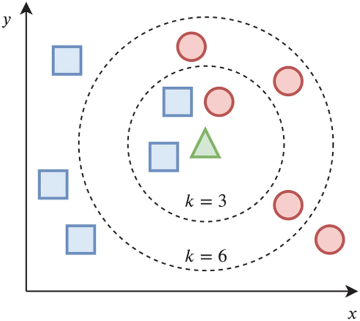
Figure 2: Illustrates its operation [40]

3.2.2 Logistic Regression Algorithm

In the last two decades, LR analysis has grown in popularity as a statistical technique in research. When the probability of a binary (dichotomous) result is to be predicted from one or more independent (predicting) factors, it is generally considered the best statistic to apply [41]. The logistic function [42] is of the form:

p(x)=11+e−(x−μ)/s(11)

where μ is a location parameter (the midpoint of the curve, where p (μ) = 1/2) and s is a scale parameter. This expression may be rewritten [42] as:

p(x)=11+e−(β0+81x)(12)

where β0 = −μ/s and is known as the intercept, and β1 = 1/s. We may define the “fit” to yk at a given xk [42] as:

pk=p(xk)(13)

Tab. 1 shows hyper parameters with the best value(s) with available range for KNN and LR algorithms.

4  Research Methodology

The methodology used in this research is to know the effect of features selection methods and data preprocessing. This is done by comparing the accuracy of data classification and the training time of the model. Three different experiments in the methods and algorithms will be applied.

The first experiment: The data sets used in this research are classified through two famous classification algorithms, namely the “LR” algorithm and the “KNN” algorithm, without preprocessing the data or applying one of the features selection methods. Fig. 3. Experiment 1: illustrates the methodology of the first experiment.

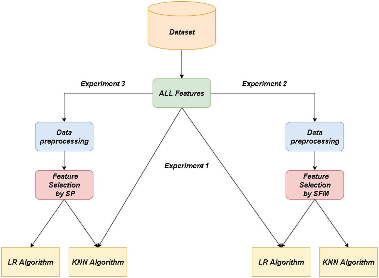
Figure 3: Architectural design of the feature selection process with classification algorithms

Experiment Two: The missing data is processed for the datasets. Also, texts are converted into numbers by “Label Encoder” method. It applies the “Standard Scaler” method to make numbers in a specified range. The best features affecting the target are selected using the “SFM” method, using the “RFI” algorithm to extract the most important features. After that, the pre-processed data is entered into the classification algorithms used in this research to know the effect of pre-processing the data, with the application of one of the selecting features methods compared to the first experiment. Fig. 3. Experiment 2: illustrates the methodology for the second experiment.

Feature Selection using “SFM” starts with determining the threshold value to give a boundary between the features to be selected and the features that will be eliminated, then all features will be sorted by gini importance score from the smallest to the largest. Furthermore, features with gini importance score that are below the threshold value will be eliminated. Selected features will be used in the “RFI”. Steps feature selection in the “SFM” method.

1.    Determine the threshold.

2.    Sort the value of the feature.

3.    Elimination the feature below the threshold.

4.    Enter selected features in Machine Learning Algorithm.

5.    Test the Performance of the Model.

The third experiment: The same as the second experiment, but the “SP” method (Select features according to a percentile of the highest scores using the “chi2” tool. The following percentages have been tried: 20%, 25%, and 30%) was used to choose the most important features, to explore the best way between them when dealing with big data analysis and visualization. Fig. 3. Experiment 3: shows the methodology of the third experiment. Experiments were evaluated by the accuracy of data classification (See Eq. (14)), model training time (It is the time it takes to train a particular model), and data reduction rate (See Eq. (15)).

Accuracy=TP+TNTP+TN+FP+FN∗100%(14)

Reductionrate=featuressubsetselectedAllfeatures(15)

5  Results

5.1 Dataset Description

This paper used eight datasets of different domains and dimensions from two main sites, the kaggle, and the uci machine learning repository. Including categorical, integer, real. The number of features of the data sets used ranges from 8 to 2001. To find out the effect of pre-processing and feature selection for high- and small-dimensional data by comparing the Model’s classification accuracy and the Model’s training time. This study aims to determine the best method among the methods used in this research to deal with the analysis and visualization of big data. Tab. 2 shows the details of the data sets in terms of the features number and the instance number for each data set, it also shows the classes number for each data set. The data was split into 20% for testing and 80% for training in all the methods implemented in this paper.

5.2 Results Analysis

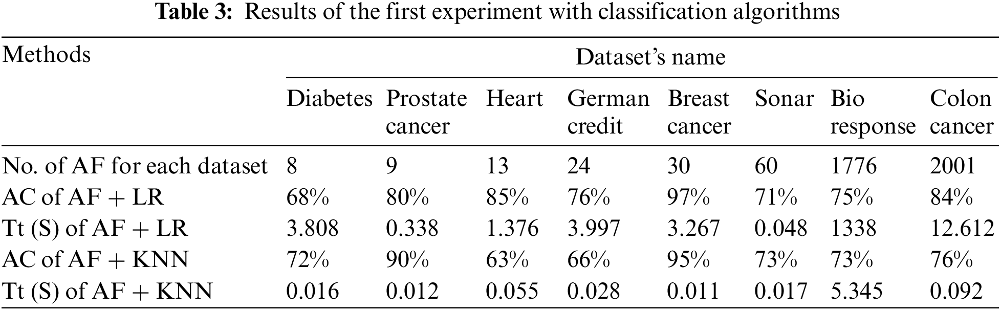
The results of the three experiments are presented in tabular form. Where, each table represents the results of an experiment. Tab. 3 presents the results of the first experiment. Where, the first row represents the number (NO.) of all features (AF) raw for each data set. The second and third row represent the results of the model’s training time in seconds (Tt (S)) and the “AC” of data classification with the “LR” algorithm.

The fourth and fifth rows represent the results of the model’s training time in seconds and the accuracy of data classification with the “KNN” algorithm (See Tab. 3).

Tab. 4 shows the results of the second experiment. Where, the first row represents the number of features extracted after applying the “SFM” method for feature selection.

The second row represents the percentage of data reduction after applying the feature selection method to all data sets.

The third and fourth rows represent the model’s training time in seconds and data classification accuracy with “LR” algorithm after applying the feature selection method.

The fifth and sixth rows represent the model’s training time in seconds and the accuracy of data classification with the “KNN” algorithm after applying the feature selection method. (See Tab. 4).

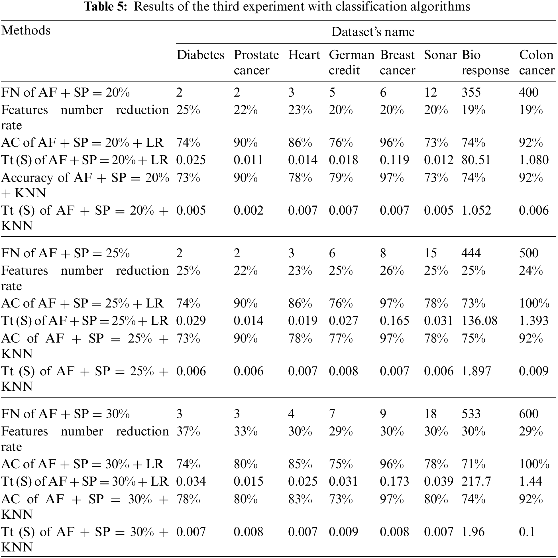
Tab. 5 shows the results of the third experiment. The “SP” method was used to determine the percentage of extraction of the best features. The experiment was carried out on three percentages (20%, 25%, and 30%).

The first part of the Tab. 5 represents the results of the 20% percentage. Where, the first row represents the features number (FN) selected when a percentage of 20%. The second row represents the features number reduction rate of data sets for the above percentage (20%). The remaining rows represent the model’s training time in seconds and data classification accuracy for the classification algorithms used in this paper.

The second part of the Tab. 5 represents the results for the 25% percentile. Where, the first row represents the features number selected when a percentage of 25%. The second row represents the features number reduction rate of data sets for the above percentage (25%). The remaining rows represent the model’s training time in seconds and data classification accuracy for the previously mentioned classification algorithms.

The third part of the Tab. 5 represents the results of the 30% percentage. Where, the first row represents the features number selected when a percentage of 30%. The second row represents the features number reduction rate of data sets for the above mentioned percentage (30%). The remaining rows represent the model’s training time in seconds and data classification accuracy for the classification algorithms used in this paper (See Tab. 5).

5.3 Discussion

To analyze the results extracted from the experiments used in this research. Several comparisons were made to get the best results. Tab. 6 shows the number of features before and after applying the feature selection methods. Where, the first row represents the number of all the raw features of the data sets. The second row represents the number of features selected after applying the “SFM” method. The remaining rows in the table represent the number of features selected after applying the “SP” method (See Tab. 6 and Fig. 4).

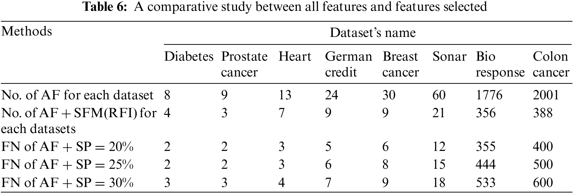
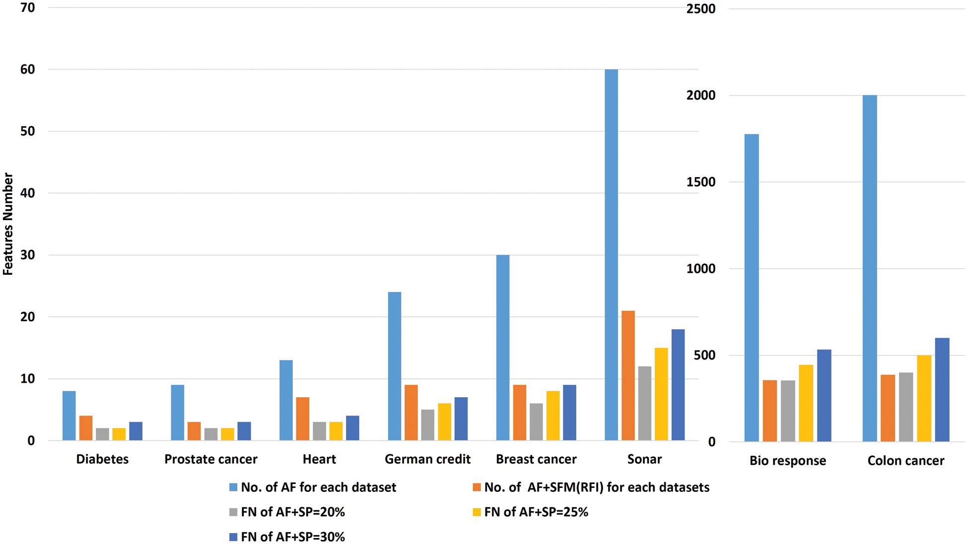
Figure 4: A comparative study between all features and features selected

Tab. 7 shows a comparison of model training time in seconds using “LR” algorithm to classify data before and after applying feature selection methods. The first row represents the training time in seconds of the model before applying the feature selection methods. The second row represents the training time in seconds of the model after applying the “SFM” method for selecting features. The remaining rows represent the model’s training time in seconds after applying the “SP” method for percentages used in the research (See Tab. 7 and Fig. 5).

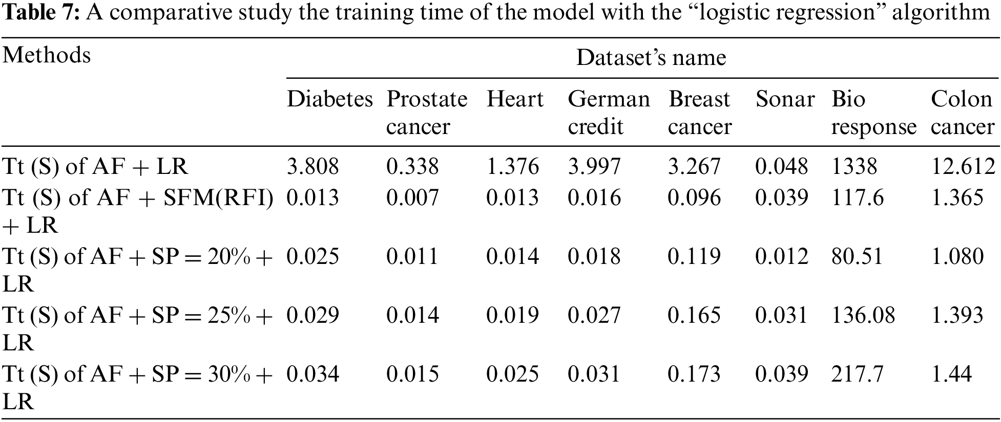
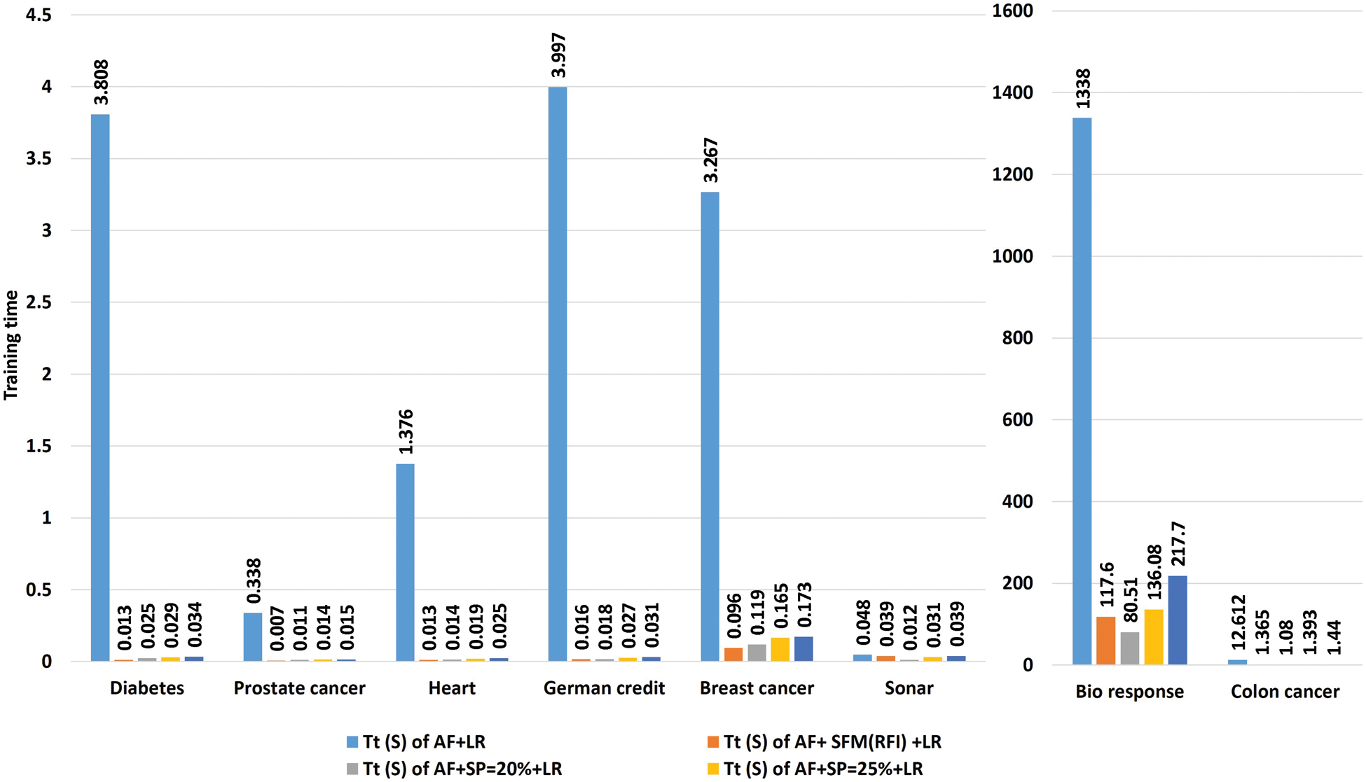
Figure 5: A comparative study the training time of the model with the “logistic regression” algorithm

Tab. 8 shows a comparison of the model’s training time in seconds using the “KNN” algorithm to classify the data before and after applying feature selection methods. The first row represents the training time in seconds of the model before applying the feature selection methods. The second row represents the training time in seconds of the model after applying the “SFM” method for selecting features. The remaining rows represent the model’s training time in seconds after applying the “SP” method for the percentages used in the research (See Tab. 8 and Fig. 6).

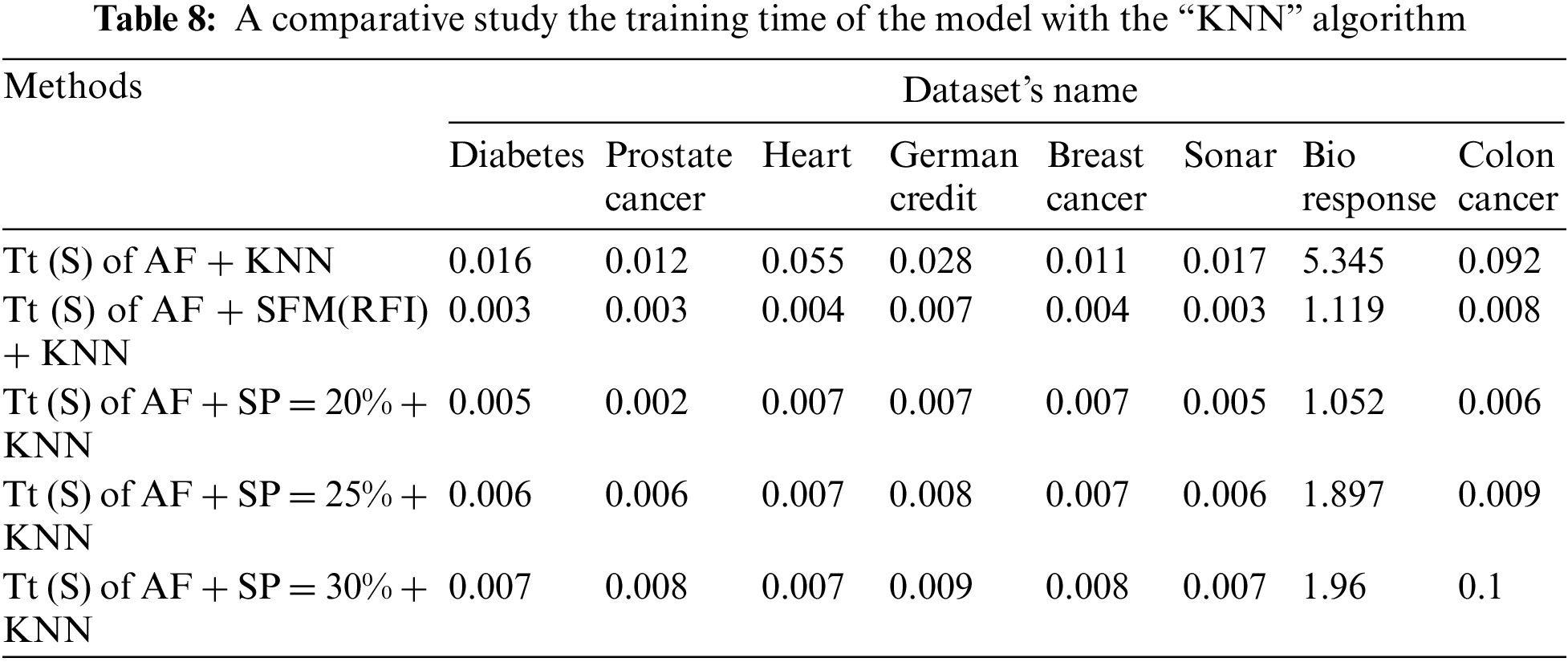
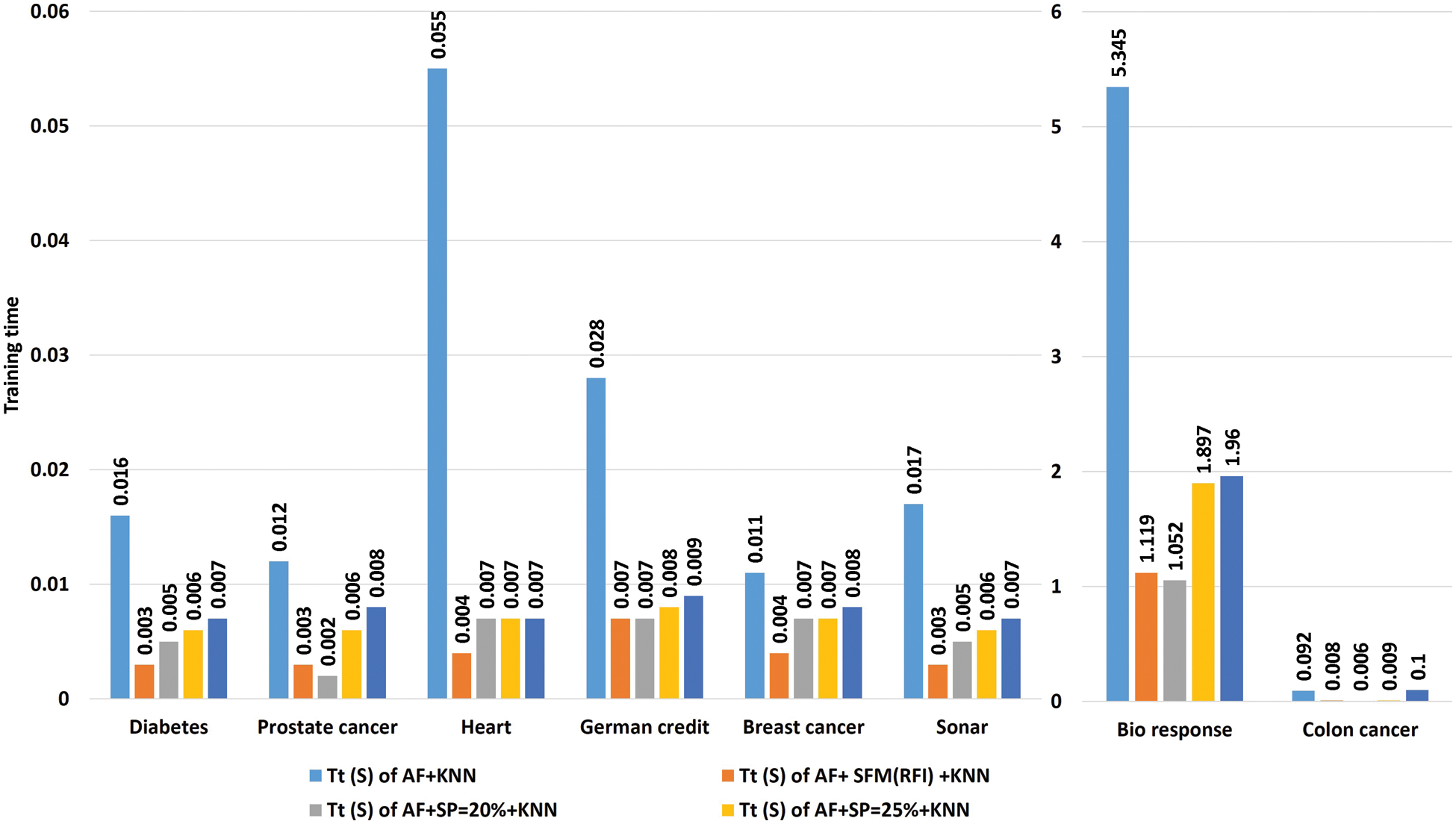
Figure 6: A comparative study the training time of the model with the KNN algorithm

Tab. 9 shows the comparison of accuracy using “LR” algorithm to classify data before and after applying feature selection methods. Where the first row represents the classification accuracy before applying feature selection methods. The second row represents the classification accuracy after applying the “SFM” method for feature selection. The remaining rows represent the classification accuracy after applying the “SP” method for percentages used in the research (See Tab. 9 and Fig. 7). The importance of these results presented is to know the effect of the feature selection methods on the accuracy of data classification using the LR algorithm.

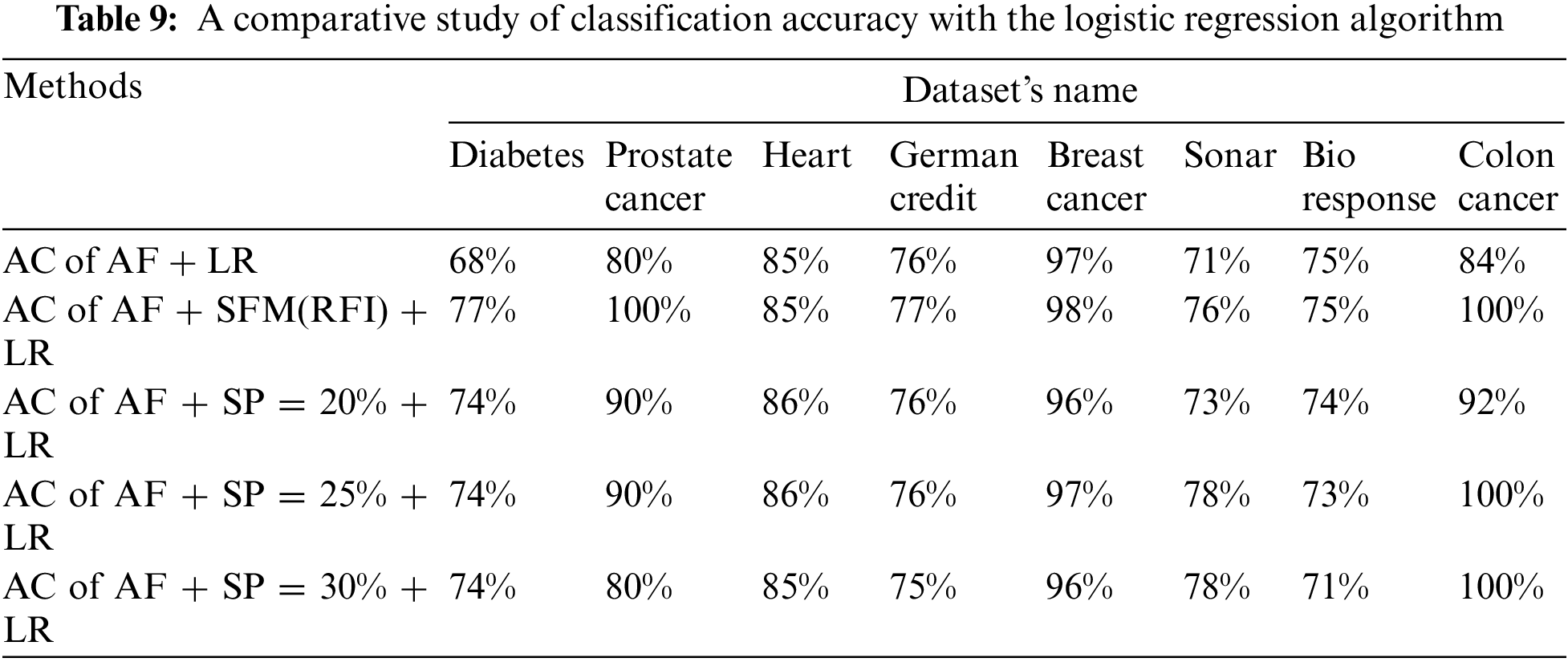
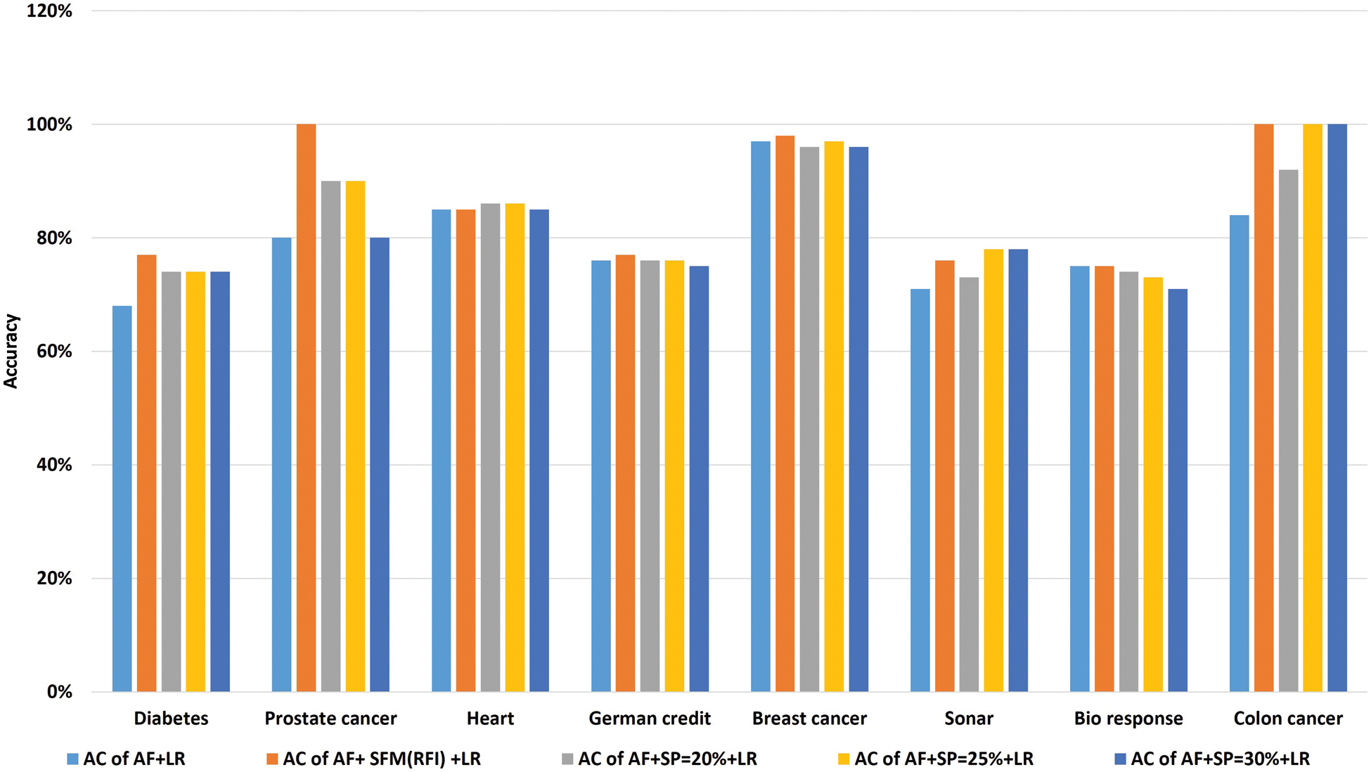
Figure 7: A comparative study of classification accuracy with the logistic regression algorithm

Tab. 10 shows the comparison of accuracy using the “KNN” algorithm to classify data before and after applying feature selection methods. Where the first row represents the classification accuracy before applying feature selection methods. The second row represents the classification accuracy after applying the “SFM” method for feature selection. The remaining rows represent the classification accuracy after applying the “SP” method for percentages used in the research (See Tab. 10 and Fig. 8). The importance of these results presented is to know the effect of the feature selection methods on the accuracy of data classification using the KNN algorithm.

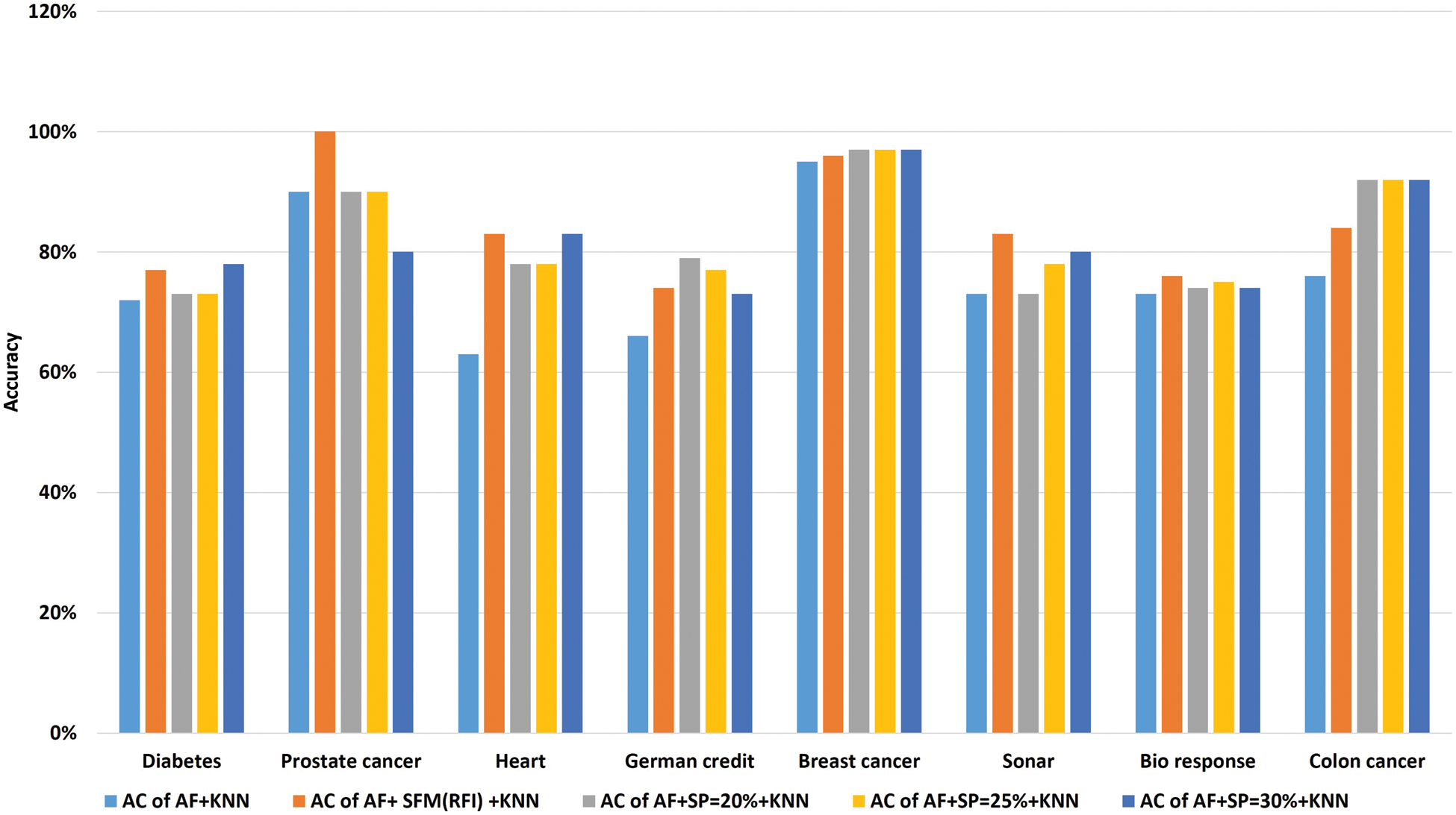
Figure 8: A comparative study of classification accuracy with the “KNN” algorithm

We conclude from these comparisons that feature selection methods reduce model training time, higher classification accuracy, and reduce data size while maintaining data quality.

Thus, we concluded that the “SFM” method for selecting features gives us better results when dealing with large data because it brings all the important features affecting the target, unlike the “SP” method because it depends on giving a certain percentage, and therefore may not bring all the features affecting the target, or it may bring advantages to it little effect. Whereas we suggest using the “SFM” method when dealing with big data analysis and visualization.

Tab. 11 shows the comparison of model classification accuracy after data preprocessing and application of “SFM” method for feature selection between logistic regression algorithm and “KNN” algorithm. (See Tab. 11). The importance of the presented results lies in knowing which algorithm gives the highest classification accuracy after applying the SFM method for feature selection.

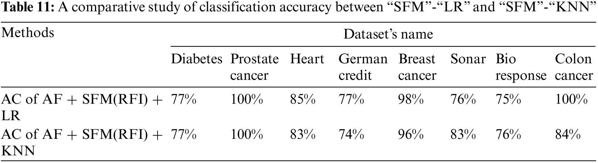
The results shown in Tab. 11 show that the classification accuracy of the two algorithms was close to each other, but the (“SFM” + “LR”) algorithm is superior to the accuracy of the KNN algorithm in most of the data sets, and this is the research proposal, called “SFMLR” (See Fig. 9).

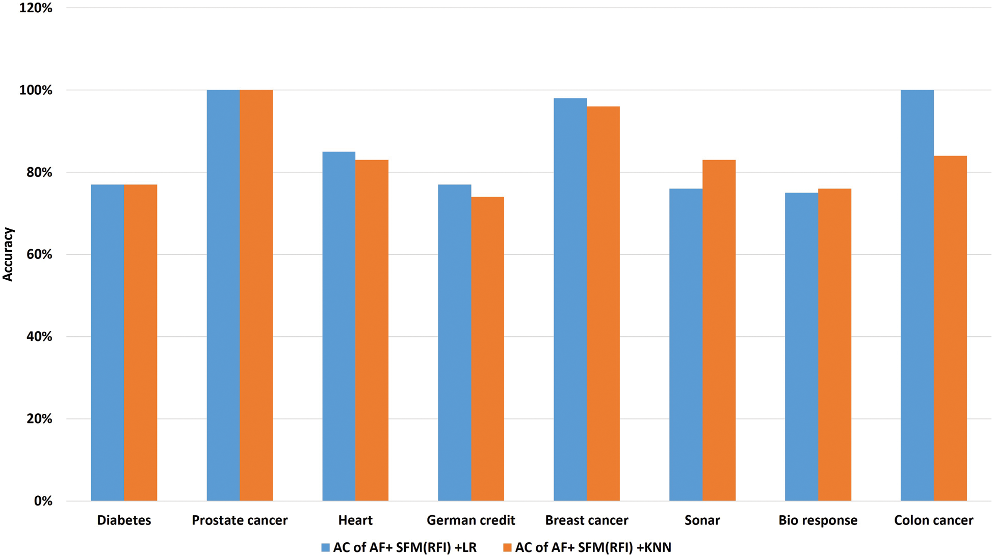
Figure 9: A comparative study of classification accuracy between “SFM”-“LR” and “SFM”-“KNN”

In addition, the recommended proposal “SFMLR” has proven its efficiency by comparing its results with the results of previous work. It turns out that our proposal often gives more accurate results. Tab. 12 shows a comparison of the results of the proposal with the results of other methods of selecting features. Thus, the number in parentheses next to each method represents the features chosen for its dependent method. This proves that the feature selection methods effectively reduce the volume of big data to analyze and visualize the results at a higher speed, accuracy, and more certainty of the effects of analyses and visualizations. Consequently, we thus faced the challenges of big data visualization by minimizing data using feature selection methods.

6  Conclusions and Future Work

By comparing the results of the experiments, the research concludes that the methods of selecting features have an effective effect in reducing the size of the data while maintaining its quality, reducing the training time of the model, and higher classification accuracy. Thus, this study contributed a proposal to address the challenges of big data visualization by using data reduction based on feature selection methods by SFM using the RFI algorithm for feature selection. With LR algorithm to classify data. The results were evaluated by accuracy, model training time, and data reduction rate. The results showed that the proposal proved to be efficient by comparing the results with the recent literature. It is recommended to use the proposal before big data visualization to get the best subset affected on the goal to help decision makers to make a more powerful and influential decision on the future of the company or organization.. In the future, suggest using genetic algorithms (GA) and particle swarm optimization (PSO) for selecting the features by the wrapper method before visualizing big data.

Acknowledgement: The authors would like to express their sincere thanks to the associate editor and the reviewers.

Funding Statement: The authors received no specific funding for this study.

Conflicts of Interest: The authors declare that they have no conflicts of interest to report regarding the present study.

References

1. R. Agrawal, A. Kadadi, X. Dai and F. Andres, “Challenges and opportunities with big data visualization,” in Proc. of the 7th Int.Conf. on Management of Computational and Collective IntElligence in Digital EcoSystems, New York, NY, USA, Medes ’15, ACM, pp. 169–173, 2015. [Google Scholar]
2. H. A. Abdelhafez and A. A. Amer, “The challenges of big data visual analytics and recent platforms,” World of Computer Science & Information Technology Journal, vol. 9, no. 6, pp. 28–33, 2019. [Google Scholar]
3. X. Hu, P. Zhou, P. Li, J. Wang and X. Wu, “A survey on online feature selection with streaming features,” Frontiers of Computer Science, vol. 12, no. 3, pp. 479–493, 2018. [Google Scholar]
4. O. A. Abd Alwahab and M. S. Abd Alrazak, “Using nonlinear dimensionality reduction techniques in big data analysis,” Periodicals of Engineering and Natural Sciences, vol. 8, no. 1, pp. 142–155, 2020. [Google Scholar]
5. B. H. Nguyen, B. Xue and M. Zhang, “A survey on swarm intelligence approaches to feature selection in data mining,” Swarm and Evolutionary Computation, vol. 54, no. 2, pp. 100663, 2020. [Google Scholar]
6. O. M. Alyasiri, Y.-N. Cheah, A. K. Abasi and O. M. Al-Janabi, “Wrapper and hybrid feature selection methods using metaheuristic algorithms for english text classification: A systematic review,” IEEE Access, vol. 10, pp. 39833–39852, 2022. [Google Scholar]
7. B. Remeseiro and V. Bolon-Canedo, “A review of feature selection methods in medical applications,” Computers in Biology and Medicine, vol. 112, no. 15071, pp. 103375, 2019. [Google Scholar]
8. H. M. Saleh, “An efficient feature selection algorithm for the spam email classification,” Periodicals of Engineering and Natural Sciences, vol. 9, no. 3, pp. 520–531, 2021. [Google Scholar]
9. W. Liu and J. Wang, “A brief survey on nature-inspired metaheuristics for feature selection in classification in this decade,” in 2019 IEEE 16th Int. Conf. on Networking, Sensing and Control (ICNSC), Banff, AB, Canada, IEEE, pp. 424–429, 2019. [Google Scholar]
10. E. Hancer, B. Xue and M. Zhang, “A survey on feature selection approaches for clustering,” Artificial Intelligence Review, vol. 53, no. 6, pp. 4519–4545, 2020. [Google Scholar]
11. I. Czarnowski and P. Jędrzejowicz, “An approach to data reduction for learning from big datasets: Integrating stacking, rotation, and agent population learning techniques,” Complexity, vol. 2018, no. 7404627, pp. 1–13, 2018. [Google Scholar]
12. S. F. Jabar, “A classification model on tumor cancer disease based mutual information and firefly algorithm,” Periodicals of Engineering and Natural Sciences, vol. 7, no. 3, pp. 1152–1162, 2019. [Google Scholar]
13. C. W. Chen, Y. H. Tsai, F. R. Chang and W. C. Lin, “Ensemble feature selection in medical datasets: Combining filter, wrapper, and embedded feature selection results,” Expert Systems, vol. 37, no. 5, pp. e12553, 2020. [Google Scholar]
14. M. Hajirahimova and M. Ismayilova, “Big data visualization: Existing approaches and problems,” Problems of Information Technology, vol. 9, no. 1, pp. 72–83, 2018. [Google Scholar]
15. D. Sridevi, A. Kumaravel and S. Gunasekaran, “A review on big data visualization tools,” IRE Journals, vol. 3, no. 7, pp. 45–49, 2020. [Google Scholar]
16. S. Arora, M. Sharma and P. Anand, “A novel chaotic interior search algorithm for global optimization and feature selection,” Applied Artificial Intelligence, vol. 34, no. 4, pp. 292–328, 2020. [Google Scholar]
17. M. Sharma and P. Kaur, “A comprehensive analysis of nature-inspired meta-heuristic techniques for feature selection problem,” Archives of Computational Methods in Engineering, vol. 28, no. 3, pp. 1103–1127, 2021. [Google Scholar]
18. S. Sharma and G. Singh, “Diagnosis of cardiac arrhythmia using swarm-intelligence based metaheuristic techniques: A comparative analysis,” EAI Endorsed Transactions on Pervasive Health and Technology, vol. 6, no. 23, pp. 1–11, 2020. [Google Scholar]
19. P. Kaur, R. Gautam and M. Sharma, “Feature selection for bi-objective stress classification using emerging swarm intelligence metaheuristic techniques,” Proceedings of Data Analytics and Management, vol. 91, no. 1, pp. 357–365, Springer, 2022. [Google Scholar]
20. L. Wang, Y. Wang and Q. Chang, “Feature selection methods for big data bioinformatics: A survey from the search perspective,” Methods, vol. 111, no. 1, pp. 21–31, 2016. [Google Scholar]
21. J. Cai, J. Luo, S. Wang and S. Yang, “Feature selection in machine learning: A new perspective,” Neurocomputing, vol. 300, pp. 70–79, 2018. [Google Scholar]
22. S. Karasu and A. Altan, “Recognition model for solar radiation time series based on random forest with feature selection approach,” in 2019 11th Int. Conf. on Electrical and Electronics Engineering (ELECO), Bursa, Turkey, IEEE, 13, pp. 8–11, 2019. [Google Scholar]
23. S. Alelyani, “Stable bagging feature selection on medical data,” Journal of Big Data, vol. 8, no. 1, pp. 1–18, 2021. [Google Scholar]
24. A. Bommert, X. Sun, B. Bischl, J. Rahnenführer and M. Lang, “Benchmark for filter methods for feature selection in high-dimensional classification data,” Computational Statistics & Data Analysis, vol. 143, no. 10, pp. 106839, 2020. [Google Scholar]
25. M. Rostami, K. Berahmand, E. Nasiri and S. Forouzandeh, “Review of swarm intelligence-based feature selection methods,” Engineering Applications of Artificial Intelligence, vol. 100, no. 1, pp. 104210, 2021. [Google Scholar]
26. J. Zhang, Y. Xiong and S. Min, “A new hybrid filter/wrapper algorithm for feature selection in classification,” Analytica Chimica Acta, vol. 1080, pp. 43–54, 2019. [Google Scholar]
27. X.-Y. Liu, Y. Liang, S. Wang, Z.-Y. Yang and H.-S. Ye, “A hybrid genetic algorithm with wrapper-embedded approaches for feature selection,” IEEE Access, vol. 6, pp. 22863–22874, 2018. [Google Scholar]
28. V. Feofanov, E. Devijver and M.-R. Amini, “Wrapper feature selection with partially labeled data,” Applied Intelligence, vol. 52, no. 3, pp. 1–14, 2022. [Google Scholar]
29. N. D. Cilia, C. De Stefano, F. Fontanella and A. S. di Freca, “A ranking-based feature selection approach for handwritten character recognition,” Pattern Recognition Letters, vol. 121, no. 2, pp. 77–86, 2019. [Google Scholar]
30. M. Huljanah, Z. Rustam, S. Utama and T. Siswantining, “Feature selection using random forest classifier for predicting prostate cancer,” in IOP Conf. Series: Materials Science and Engineering, Malang, Indonesia, IOP Publishing, 546, pp. 52031, 2019. [Google Scholar]
31. U. M. Khaire and R. Dhanalakshmi, “Stability of feature selection algorithm: A review,” Journal of King Saud University-Computer and Information Sciences, vol. 34, no. 4, pp. 1060–1073, 2019. [Google Scholar]
32. G. Chandrashekar and F. Sahin, “A survey on feature selection methods,” Computers & Electrical Engineering, vol. 40, no. 1, pp. 16–28, 2014. [Google Scholar]
33. A. Kumar and T. V. Kumar, “Multi-objective big data view materialization using MOGA,” International Journal of Applied Metaheuristic Computing (IJAMC), vol. 13, no. 1, pp. 1–28, 2022. [Google Scholar]
34. N. Zhao, “Credibility evaluation of web big data information based on particle swarm optimization,” Journal of Web Engineering, vol. 21, no. 2, pp. 405–424, 2022. [Google Scholar]
35. Y. Saeys, I. Inza and P. Larranaga, “A review of feature selection techniques in bioinformatics,” Bioinformatics, vol. 23, no. 19, pp. 2507–2517, 2007. [Google Scholar]
36. N. Almugren and H. Alshamlan, “A survey on hybrid feature selection methods in microarray gene expression data for cancer classification,” IEEE Access, vol. 7, pp. 78533–78548, 2019. [Google Scholar]
37. V. Bolón-Canedo, N. Sánchez-Marono, A. Alonso-Betanzos, J. M. Benítez and F. Herrera, “A review of microarray datasets and applied feature selection methods,” Information Sciences, vol. 282, no. 3, pp. 111–135, 2014. [Google Scholar]
38. L. Jiao, X. Geng and Q. Pan, “BP $ k $ NN: $ k $-nearest neighbor classifier with pairwise distance metrics and belief function theory,” IEEE Access, vol. 7, pp. 48935–48947, 2019. [Google Scholar]
39. I. Iswanto, T. Tulus and P. Sihombing, “Comparison of distance models on K-nearest neighbor algorithm in stroke disease detection,” Applied Technology and Computing Science Journal, vol. 4, no. 1, pp. 63–68, 2021. [Google Scholar]
40. J. Vieira, R. P. Duarte and C. H., “Neto, kNN-STUFF: KNN streaming unit for fpgas,” IEEE Access, vol. 7, pp. 170864–170877, 2019. [Google Scholar]
41. E. Y. Boateng and D. A. Abaye, “A review of the logistic regression model with emphasis on medical research,” Journal of Data Analysis and Information Processing, vol. 7, no. 4, pp. 190–207, 2019. [Google Scholar]
42. M. A. Aljarrah, F. Famoye and C. Lee, “Generalized logistic distribution and its regression model,” Journal of Statistical Distributions and Applications, vol. 7, no. 1, pp. 1–21, 2020. [Google Scholar]
43. M. F. Dzulkalnine and R. Sallehuddin, “Missing data imputation with fuzzy feature selection for diabetes dataset,” SN Applied Sciences, vol. 1, no. 4, pp. 1–12, 2019. [Google Scholar]
44. R. A. Ibrahim, A. A. Ewees, D. Oliva, M. Abd Elaziz and S. Lu, “Improved salp swarm algorithm based on particle swarm optimization for feature selection,” Journal of Ambient Intelligence and Humanized Computing, vol. 10, no. 8, pp. 3155–3169, 2019. [Google Scholar]
45. A.-A. A. Mohamed, S. Hassan, A. Hemeida, S. Alkhalaf, M. Mahmoud et al., “Parasitism-Predation algorithm (PPAA novel approach for feature selection,” Ain Shams Engineering Journal, vol. 11, no. 2, pp. 293–308, 2020. [Google Scholar]
46. S. B. Sakri, N. B. A. Rashid and Z. M. Zain, “Particle swarm optimization feature selection for breast cancer recurrence prediction,” IEEE Access, vol. 6, pp. 29637–29647, 2018. [Google Scholar]
47. A. N. Alharbi and M. Dahab, “An improvement in branch and bound algorithm for feature selection,” Int. J. Inf. Technol. Lang. Stud, vol. 4, no. 1, pp. 1–11, 2020. [Google Scholar]
48. M. A. Rahman and R. C. Muniyandi, “Feature selection from colon cancer dataset for cancer classification using artificial neural network,” International Journal on Advanced Science, Engineering and Information Technology, vol. 8, no. 4–2, pp. 1387–1393, 2018. [Google Scholar]
Cite This Article
Copyright © 2023 The Author(s). Published by Tech Science Press.
This work is licensed under a Creative Commons Attribution 4.0 International License , which permits unrestricted use, distribution, and reproduction in any medium, provided the original work is properly cited.
Downloads
Citation Tools