Numerical Comparison of Shapeless Radial Basis Function Networks in Pattern Recognition

1  Introduction

Under the framework of intelligent machines, the ability to classify or recognise patterns through the structure of neural networks is highly essential and challenging in a wide range of applications including biomedical and biology, social medial intelligence (SMI), video surveillance, intelligent retail environment and digital cultural heritage [1,2]. Several concepts or methodologies have been proposed and studied during the past decade where networks can be roughly categorised into two main classes; deep learning and shallow learning, the name represents the number of layers involved in the network. Some recent successes of deep networks to be recommended include the classification of Alzheimer’s diseases and mild cognitive impairment [3] and the classification of COVID-19 based on CT images [4]. On the other hand, the shallow structure has also been comparatively studied and applied in a variety of contexts [5]. One of the popular shallow architectures is the use of the so-called ‘radial basis function (RBF)’, a type of multivariate function.

RBF neural networks were originally introduced in [6,7] and have been extensively investigated ever since such as the classification and prediction [8–10], those in agriculture [11,12], finance [13], and medicine [14], to mention only a few, confirming the versatile and promising aspect of RBF networks in general. When it comes to applying RBF networks, two traditional and well-known choices are the Gaussian (GA) and the Multiquadric (MQ), in which a so-called ‘shape parameter’ occurs. It is this shape parameter that is known to play a highly crucial role in determining the quality of the networks. Specifying a proper value of this shape is rather complicated. It is known to strongly depend on several factors including the number and the distribution manner of nodes, the size of the problem domain, the numerical and mathematical procedures involved in the process, etc. Apart from GA and MQ, the pain of shape-determining also persists for all shape-contained RBF types making their use not as practical. The challenge of searching for an optimal shape parameter (if any and for each shape-contained RBF) has consequently been one of the active research areas related to RBFs’ applications and some are briefly introduced here.

In 2019, Krowiak et al. [15] proposed a scheme employing a heuristic that relates the condition number to computational precision and searches for the largest value of this parameter that still ensures stable computation using geometrical dependence. A year later, Zheng et al. [16] used the approximation error of the least-squares to measure the shape parameter of the radial basis function and proposed a corresponding optimization problem to obtain the optimal shape parameter. Later in 2021, Kaennakham et al. [17] compared two interesting forms of shape (one is in exponential base and the other in trigonometric) in the context of recovering functions and their derivatives, and also in this year, Cavoretto et al. [18] proposed finding an optimal value of the shape parameter by using leave-one-out cross-validation (LOOCV) technique combined with univariate global optimization methods. Despite the broad range of research under this path, the topic is still highly problem-dependent, i.e., one reasonable good shape for a certain task might be useless for others when problem configuration changes.

Alternatively to shape-contained RBFs and to avoid the demerits mentioned so far, RBFs containing no shapes, referred to as ‘shapefree’ or ‘shapeless’ have recently been paid attention to. Recent work can be found in [19] where the authors attempted to approximate the solution of PDEs using RBF with no shapes. The application in the pattern recognition context, to our knowledge, has not been explored as much and our preliminary investigations have strongly been promising when shapeless RBFs are in use [20,21]. Therefore, to encourage the research under this path and extend the scope of our previous works, this work focuses on a numerical investigation of the effectiveness of sixteen shapeless RBFs. The challenge is carried out under the context of pattern recognition through the structure of radial basis function neural networks (RBF-NNs) applied in conjunction with the Representational Capability (RC) algorithm (full detail is provided in Section 2). The effectiveness is validated based on several criteria including accuracy, condition number, CUP-time and storage, user interference, and sensitivity to other factors.

Three main contributions this work is aimed to make are;

•   To demonstrate the application of the Representational Capability (RC) algorithm in RBF neural networks for pattern recognition problems.

•   To provide more information on how reliable shapeless RBFs can be for pattern recognition problems, as compared to one of the popular choices of shape-contained RBFs.

•   To compare the effectiveness of sixteen selected shapeless RBFs under the same problem configuration.

It is hoped that with a good choice of shapeless RBF, one should be able to achieve high-quality results without suffering the pain caused by choosing the shape. Section 2 provides the problem statement with all crucial components before the computational algorithm with all the criteria being declared in Section 3. Section 4 then reports the essential results obtained and the main conclusions are drawn in Section 5.

2  Methodology and Problem Statement

2.1 Pattern Recognition with Radial Basis Functions Neural Networks

For the task of pattern recognition, the so-called ‘training datasets’ undergo a process designed to construct a model or a mapping (if any) that is hoped to best represent the rest of the data or ‘testing datasets’. The process occurring in the middle is the main challenge as it is typically unknown. Both sets of data can be of the following form.

D={(xi,yi)|xi∈Rd,yi∈R,i=1,2,⋯,n}(1)

where xi are inputs and yi are the corresponding outputs. The main task is to find a mapping D from the d−dimensional input space to 1−dimensional output space.

The model structure of a typical radial basis function network is depicted in Fig. 1, when a data set {(xi,yi)}i=1n is given and the model searches for the corresponding output estimate y^ for the input vector x, represented by functional form:

y^=f(x)=∑j=1mwjϕj(x)=∑j=1mwjϕj(||x−μj||2)(2)

where ||−||2 is the Euclidean distance norm, ϕ(⋅) is a basis function, m is the number of basis functions, n is the number of input data, μj are the centres of j-th basis functions, and wj are the weights associated with the j-th basis function. (note that m≤n)

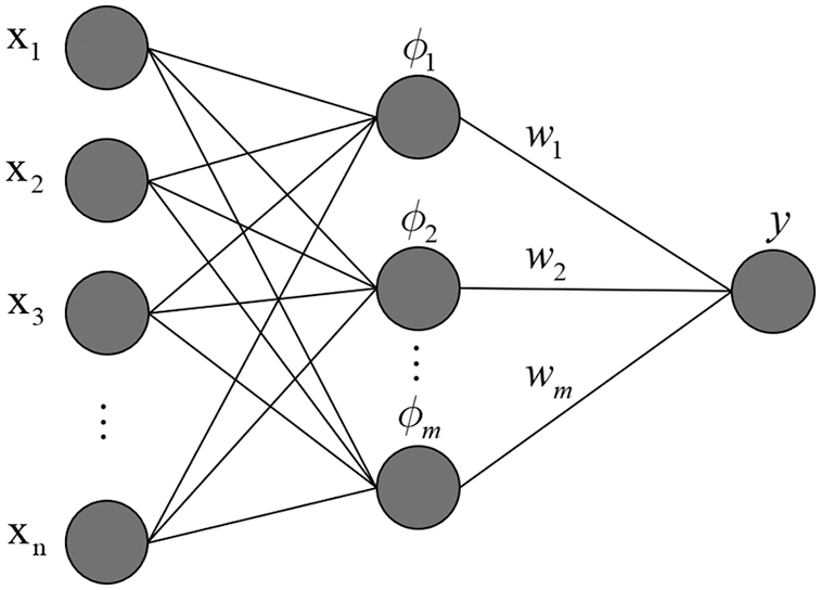
Figure 1: Typical radial basis function (RBF) neural network structure

2.2 The Selected Shapeless RBFs

Sixteen forms of shapeless RBFs are paid attention to in this work and they are listed in Table 1. For the sake of comparison, the well-known shape-contained RBF namely ‘Multiquadric, MQ’ is also parallelly studied where the shape choosing scheme proposed by Carlson, 1991 [22] is used. Differences in the curve profiles for each shapeless RBF can be seen and noticed in Fig. 2.

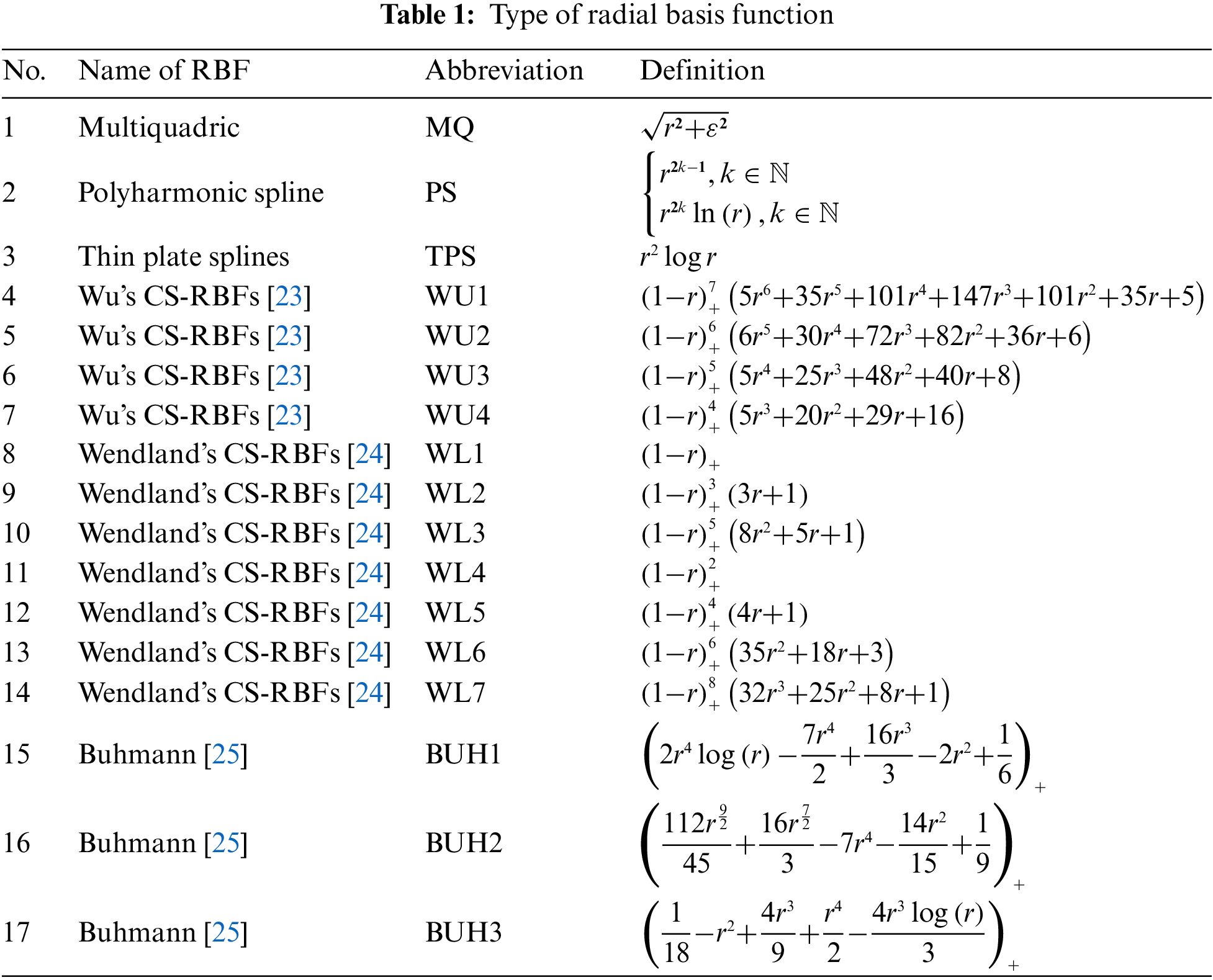
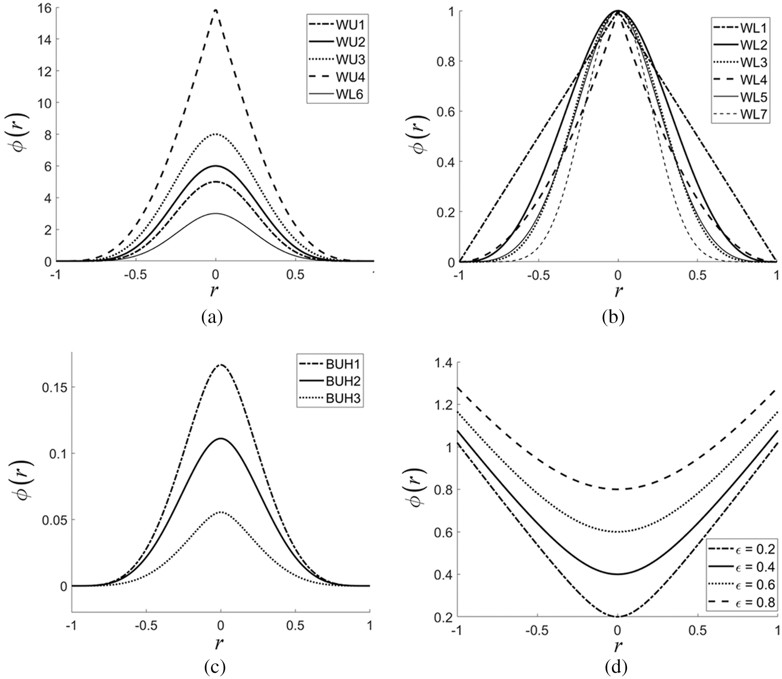
Figure 2: One-dimensional curve for each type of RBFs under this investigation; (a–c) of those containing no shapes (or shapeless), and (d) the famous MQ with different shape values

2.3 The Representational Capability (RC) Algorithm

The Representational Capability (RC) algorithm as proposed by Shin et al. (2000) [26] is a method to drag out only meaningful and significant information from the interpolation matrix when RBF is in use. For a given set of input data {xi,yi}i=1n, for the sake of the completeness of the work, the algorithm is elaborated with the following steps.

Step 1: Select a value for the width (or the shape parameter) (ε), and the effect of noise (δ) which δ is usually taken to be 0.1% to 1.0%, then construct the interpolation matrix G. For example, if the Gaussian basis function is used, so that

G=[g11g12⋯g1ng21g22⋯g2n⋮⋮⋱⋮gn1gn2⋯gnn](3)

where gij=exp⁡(−||xi−xj||2/2ε2) for i,j=1,2,…,n.

Step 2: Determine the number of basis functions (m) by applying the singular value decomposition procedure to the interpolation matrix G. This yields a diagonal matrix (namely V) of singular values s1≥s2≥⋯≥sn≥0. From this step, m can be determined from the following expression:

m=max0≤i≤n{i|si+1≤s1×δ100}.(4)

Step 3: Determine the centres of basis function (μ). This is done by partitioning matrix V from singular value decomposition of the interpolation matrix G, as follows:

V=[v11v12v21v22]n×n(5)

Next, generate matrix V′=[v11Tv21T]m×n and apply QR factorization with column pivoting of matrix V′. Then compute XTP and choose the first m elements in XTP be the centres of basis function which are:

μ={μj}j=1m(6)

Step 4: Compute the weight parameters from the basis function (w). Consider,

ϕ=[ϕi,j],Fori=1,2,…,nandj=1,2,…,m.(7)

Compute the m weights using the following expression.

w=ϕ+y(8)

where ϕ+ denoted the pseudo inverse of ϕ.

3  Experimental Setups

3.1 Performance Criteria

As previously mentioned, all sixteen shapeless RBFs are comparatively and numerically investigated. Therefore, proper and all-around effectiveness criteria are required and they are listed below.

•   Accuracy: This process is carried out using the following two error norms.

LRMSE=[1N∑i=1N(yext.(xi,yi)−yappx.(xi,yi))2]1/2(9)

and

L∞=max1≤i≤N|yext.(xi,yi)−yappx.(xi,yi)|.(10)

•   Condition number: The system can be solvable if the collocation matrix, φ, has an inverse and this can be indicated by the means of its condition number (Condδ(−)) expressed as follows.

Condδ(φ)=||φ||δ||φ−1||δ(11)

The trending behaviour of this number is also recorded throughout this experiment, providing information on the solvability, [27], of the collocation matrix for future uses.

•   CPU-time: With less amount of time required for the computational process, a method would be more desirable. The ‘tic-toc’ command in MATLAB is employed for this task.

•   Storage requirement: Each computation step involved in the algorithm should ideally take as least amount of storage space as possible. For the sake of fairness, all experiments are carried out on the same computer (Intel(R) Core(TM) i7-1065G7 CPU @ 1.30 GHz 1.50 GHz with RAM 16.00 GB and 64-bit Operating System).

•   User’s Interference: A good algorithm should be able to process entirely by itself, no human interruption or judgments should be involved. This is all for future practical uses.

•   Sensitivity to parameters: A small change in parameters embedded in the process should have as little effect as possible on the overall performance. Methods containing no parameters would be best in practice.

•   Ease of implementation: Once the desirable method has been proven with small test models, it is then anticipated to successfully be implemented to larger problems with no difficulties (in terms of both mathematical structures and programming/coding).

3.2 Dataset-Partitioning Manners

For the data-partitioning process, the suggestion provided by Lazzaro et al. (2002) [28] is followed here with the information described as follows.

3.2.1 The Training Datasets

Two datasets with the size of 50×50 nodes are generated within a [0,1]×[0,1] domain; uniformly and randomly as shown in Fig. 3. These sets of data are to be used as a ‘Training Dataset’ for all numerical experiments in this study.

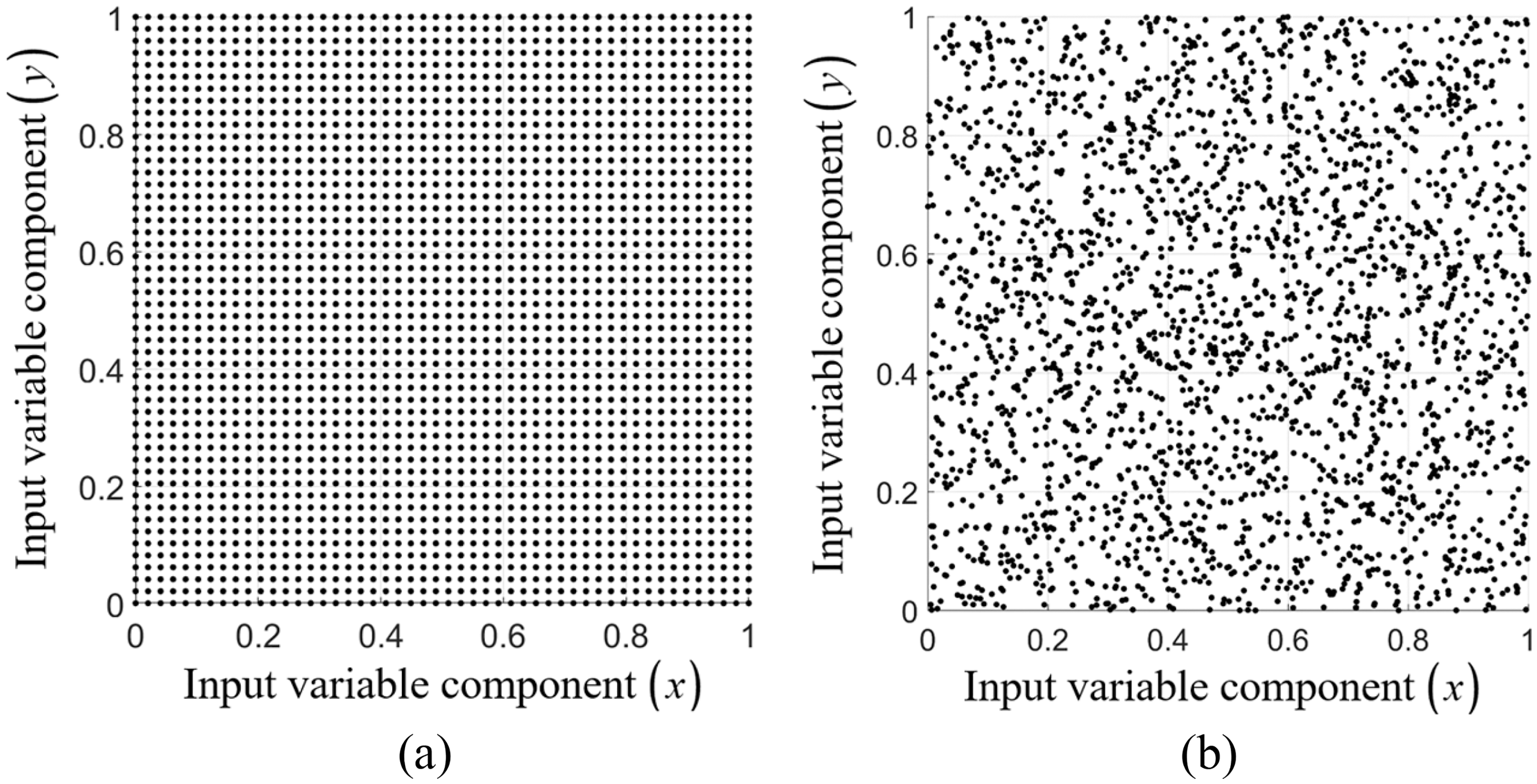
Figure 3: (x,y)−Node distribution manners for training datasets using 50×50 nodes: (a) uniformly (Ufm.), and (b) non-uniformly (randomly, Rdm.)

3.2.2 The Testing Datasets

To monitor and record the effectiveness of each RBF type, three large datasets are generated within the same domain in both manners uniformly (Ufm.) and randomly (Rdm.), and they contain 10000, 20164, and 30276 nodes [28].

4  Numerical Experiments, Results, and General Discussion

In this section, two well-known benchmarking test cases are numerically experimented with using all the RBF forms mentioned above. Nevertheless, with the limitation of the space, only those significant and relevant results are being mentioned, illustrated, and discussed.

4.1 Experiment 1

This first experiment is concerned with one of the most well-known testing functions invented by Franke in 1982 [29] and is to be referred to as ‘Franke’s function’ hereafter. The expression of the function is as follows:

z=f(x,y)=0.75exp⁡(−(9x−2)2+(9y−2)24)+0.75exp⁡(−(9x+1)249−9y+110)+0.5exp⁡(−(9x−7)2+(9y−3)24)−0.2exp⁡(−(9x−4)2−(9y−7)2)(12)

4.1.1 Performance at SNR=30

The results validation for all RBFs for this first case is to be numerically investigated at two different noise levels (SNR); SNR=15 and 30, as illustrated in Figs. 4 and 7.

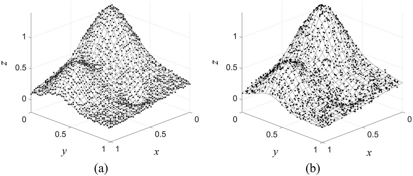
Figure 4: Noised-z(x,y) training datasets with SNR=30 based on two manners of distribution of {(x,y)}: (a) uniformly and (b) non-uniformly (randomly)

4.1.2 Performance at SNR=15

As can be seen in Figs. 4 and 7, the accuracy measured by both L∞ and LRMSE from both cases of node distribution manners slightly decreases with the increase of noise variance. This is not surprising as the pattern becomes more complicated with data being more disturbed by noise.

In terms of the number of basis functions (m) generated by the RC-algorithm, at SNR=30 and with comparatively low values of L∞, LRMSE, and Condδ(−), it is found that m=87, m=100 and m=83 are reproduced for WU3, WL5, and BUH2, respectively. This figure can be seen as a good success of these RBFs, considering 2,500 original nodes, while good accuracy is still achievable (see Tabls. 2 and 4). Table 3 also shows a similar figure for these RBFs at SNR=30 confirming their potential for further uses. The ability to preserve the data’s pattern while using a small number of nodes is desirable for any kind of RBF in practical applications. The small number in m also strongly affects both CPU time and storage required for each computation process as clearly seen in Figs. 5 and 6 for SNR=30 and Figs. 8 and 9 for SNR=15.

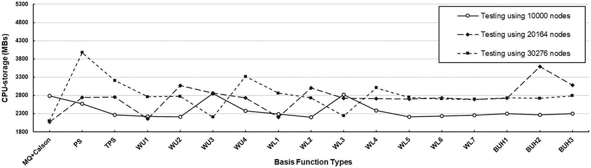
Figure 5: CPU-storage measurement observed at three different sizes of testing datasets with uniform node distribution using SNR=30

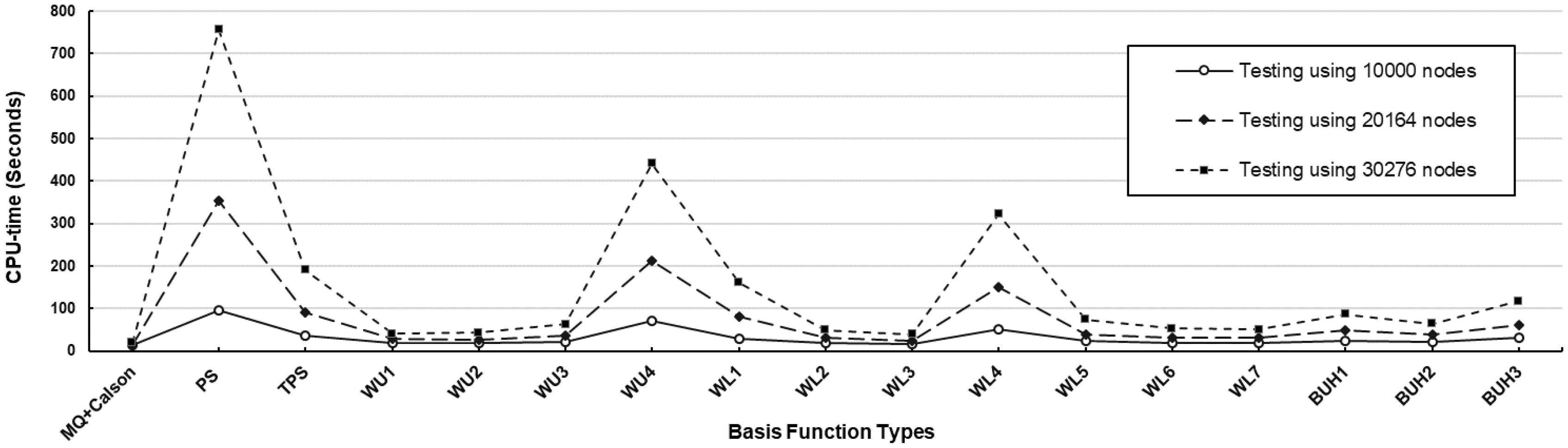
Figure 6: CPU-time measurement observed at three different sizes of testing datasets as uniform node distribution using SNR=30

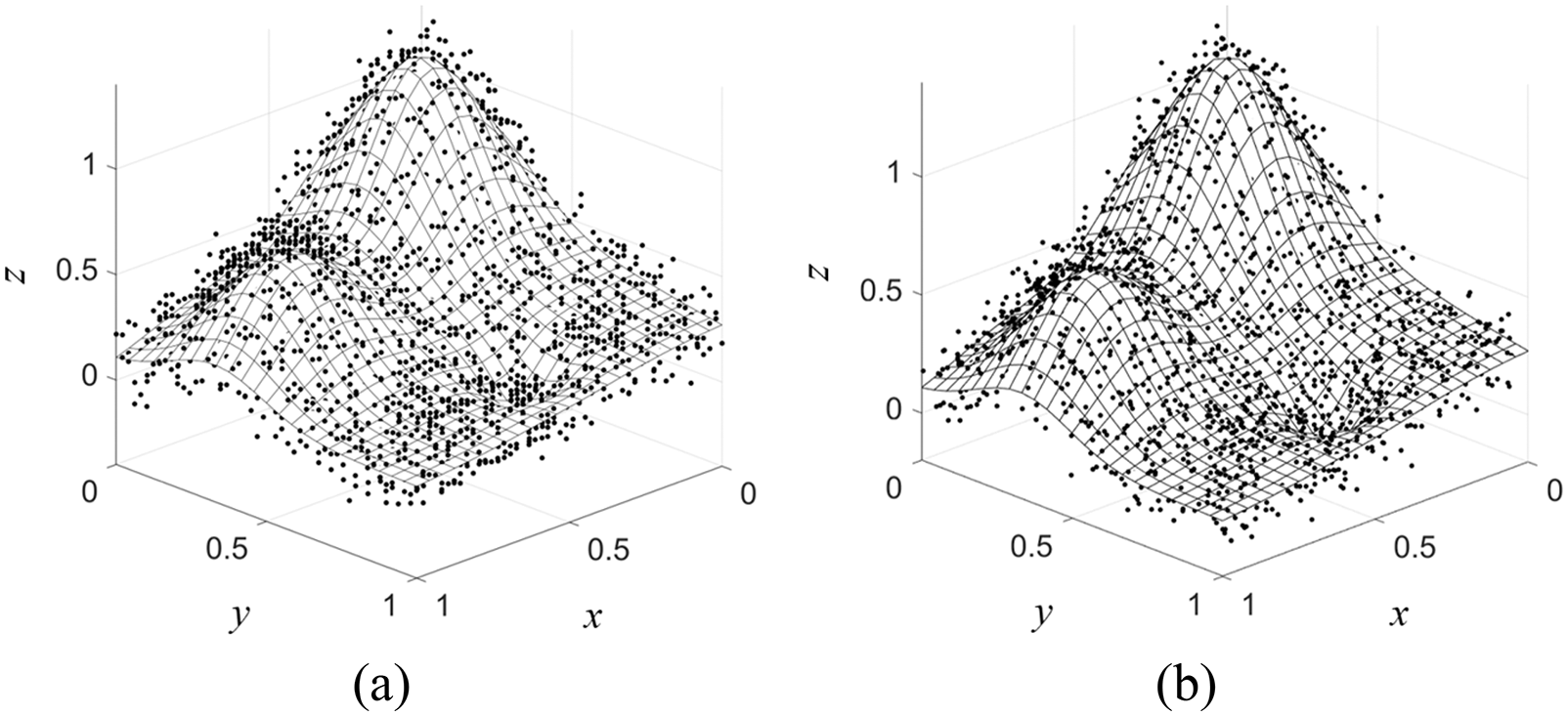
Figure 7: Noised-z(x,y) training datasets with SNR=15 based on two manners of distribution of {(x,y)}: (a) uniformly and (b) non-uniformly (randomly)

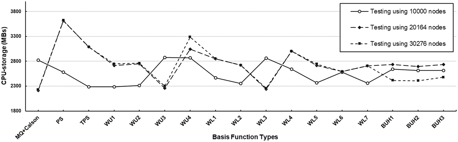
Figure 8: CPU-storage measurement observed at three different sizes of testing datasets with random node distribution using SNR=15

Figure 9: CPU-time measurement observed at three different sizes of testing datasets with random node distribution using SNR=15

4.2 Experiment 2

For the second test case, we study one of the functions called F7 in the investigation nicely carried out by Renka et al. [30], (and shall be referred to as ‘F7’ in this work as well). The function is defined as follows.

z=f(x,y)=2cos⁡(10x)sin⁡(10y)+sin⁡(10xy)(13)

Similar to the first experiment, two different noise levels or SNR (SNR=15 and 30) are under investigation with their node distributions are illustrated in Figs. 10 and 13, respectively.

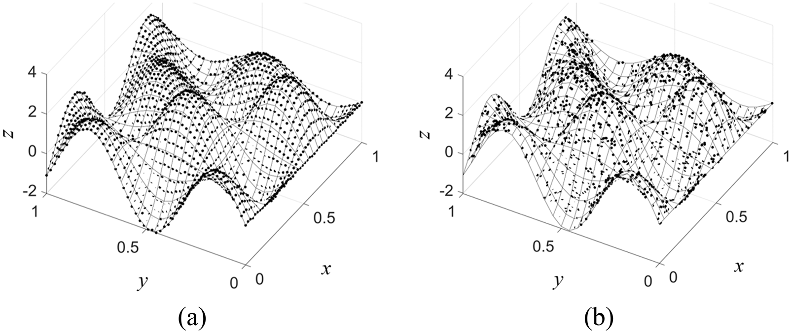
Figure 10: Noised-z(x,y) training datasets based on two manners of distribution of {(x,y)}: (a) uniformly and (b) non-uniformly (randomly)

4.2.1 Performance at SNR=30

4.2.2 Performance at SNR=15

With the results obtained in these cases, shown in Tables 5–7, together with information provided in Figs. 11 and 12, it has been observed that the overall trends in accuracy (both L∞ and LRMSE) are similar to those discovered in the first experiment (with F1) where some smaller errors are noticed in the cases of WL6 and WL7. Moreover, the similarity to the first experiment in terms of the number of basis functions (m) produced by each shapeless RBF after undergoing the RC algorithm is also noticeable here. This is since with no parameter involved these values are dependent only on the distance between two nodes. In the case of MQ, nevertheless, with different values of shape parameters generated by the Carlson algorithm, the change in the number of basis functions (m) shall be anticipated.

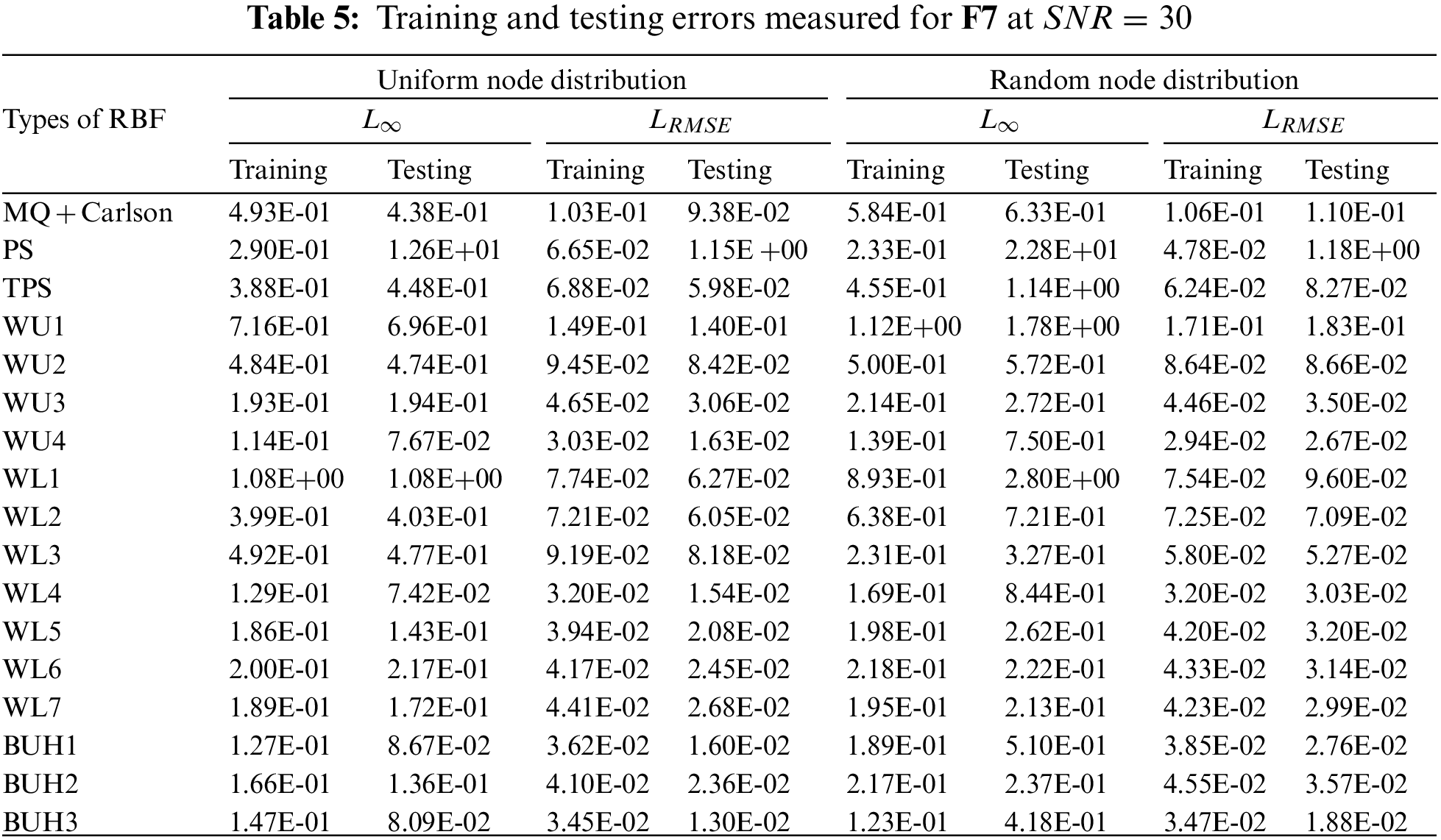
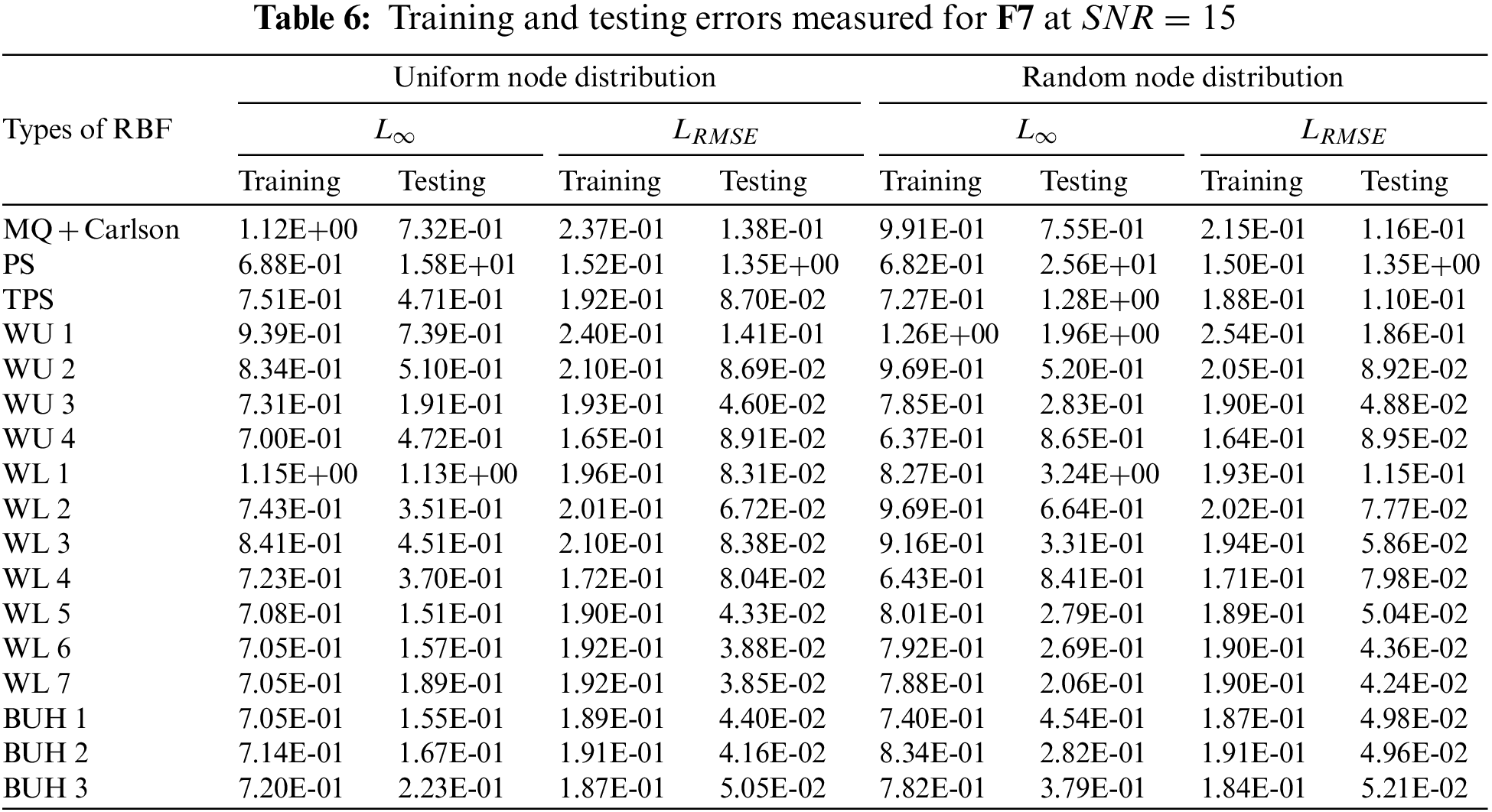
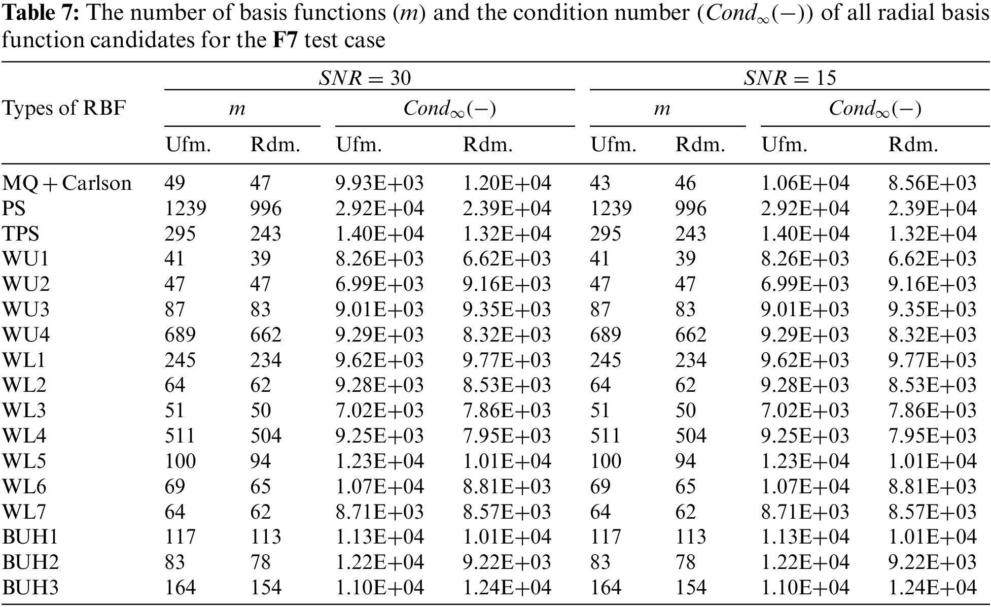
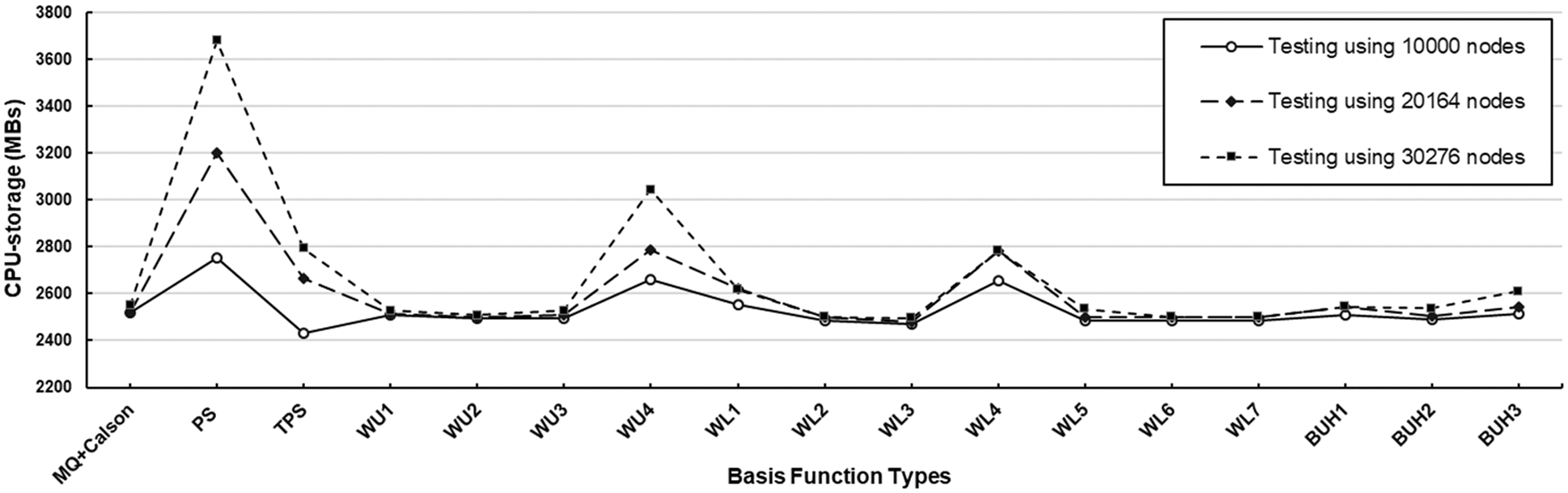
Figure 11: CPU-storage measurement observed at three different sizes of testing datasets with uniform node distribution using SNR=30

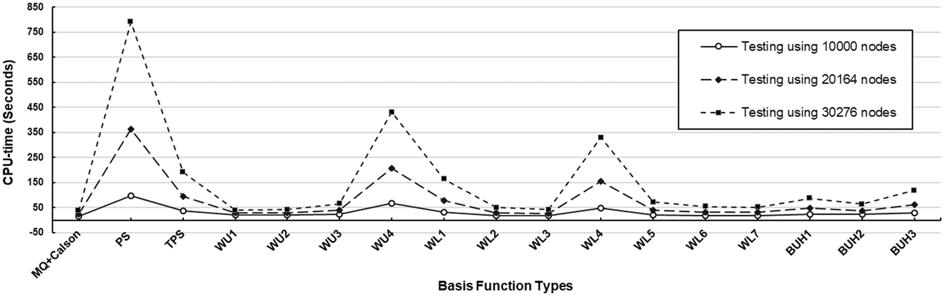
Figure 12: CPU-time measurement observed at three different sizes of testing datasets with uniform node distribution using SNR=30

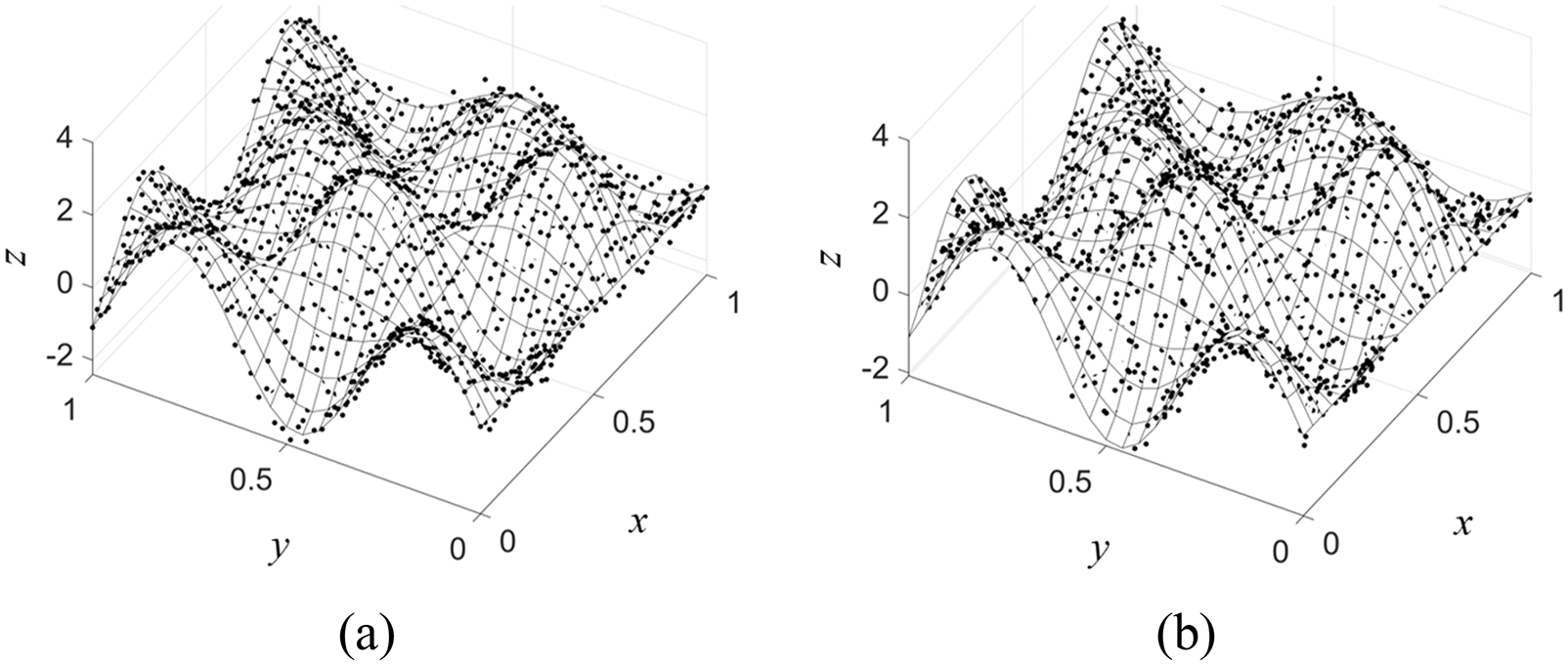
Figure 13: Noised-z(x,y) training datasets based on two manners of distribution of {(x,y)}: (a) uniformly and (b) non-uniformly (randomly)

From all the numerical results obtained so far and in addition to the criteria stated, it has to be acknowledged that ‘underfitting and overfitting’ is another crucial figure to be considered. Regarding all cases, a significant reduction in accuracy, measured by both error norms, produced by PS type of RBF strongly indicates its overfitting nature and shall not be recommended for practical uses. On the other hand, WL5, BUH1, WU3, and BUH2 are seen to be slightly underfitting for both numerical demonstrations. The best types of RBF in terms of this aspect are WU1, WU2, WL1, WL4, and MQ.

5  Conclusions

This work aims to provide insights into the use of sixteen forms of radial basis function (RBF) containing no shape parameter, so they are referred to as ‘shapeless RBFs’. The challenge under the main experiment is the problem of pattern recognition through neural networks computation process and architecture. The ability to deal with large and noised datasets of each shapeless RBF is measured under several criteria against the well-known shape-containing RBF called multiquadric (MQ). Two testing functions are tackled numerically and important findings observed (based on each criterion) are listed below.

1) Accuracy (L∞ and LRMSE): The best three shapeless RBFs are WL6, WL7, and BUH3, whereas PS, WU1, and MQ are found to produce the least accurate results.

2) The condition number (Cond∞(−)): The best three are WU1, WU2, and WL3 with the comparatively worse ones being PS, TPS, and WL5.

3) In terms of CPU (time and storage) and also the number of basis functions (m): MQ, WL3, and WL6 are seen to be the most desirable whereas PS, WU4, and WL4 are not so promising under these criteria.

4) User’s Interference: It is obvious that as long as no parameter-turning process is required, there is no need to interfere with the algorithm and this is one desirable aspect of using shapeless RBF. This is also the case for the sensitivity-to-parameter criteria.

5) Ease of implementation: It is observed that all shapeless RBF types under this work are equally simple when it comes to implementing the scheme. For MQ, on the other hand, an additional coding routine may be needed for the process of a reliable shape searching procedure, as is the case in this investigation for the Carlson algorithm.

Together with the ‘overfitting and underfitting’ aspect, this work suggests that shapeless RBFs from Wu’s and Wendland’s families are highly promising, whereas the rest forms are still skeptical for practical uses. Apart from this useful piece of information for pattern recognition application, it might be considered a weakness of the work that the figure discovered so far may change when dealing with other kinds of applications such as direct interpolation, function approximation, and recovery, as well as solving different equations (DEs) under the concepts of meshless or meshfree methods. Furthermore, other kinds of node distribution of sizes may result in different aspects. This is all set as our future research direction and is highly recommended for interested researchers to further explore.

Funding Statement: The authors received funding for this study from the Institute for the Promotion of Teaching Science and Technology, under the Development and Promotion of Science and Technology Talent Project (DPST), Thailand.

Conflicts of Interest: The authors declare that they have no conflicts of interest to report regarding the present study.

References

1. M. Parasher, S. Sharma, A. K. Sharma and J. P. Gupta, “Anatomy on pattern recognition,” Indian Journal of Computer Science and Engineering (IJCSE), vol. 2, no. 3, pp. 371–378, 2011. [Google Scholar]
2. M. Paolanti and E. Frontoni, “Multidisciplinary pattern recognition applications: A review,” Computer Science Review, vol. 37, pp. 1–23, 2020. [Google Scholar]
3. S. Fouladi, A. A. Safaei, N. Mammone, F. Ghaderi and M. J. Ebadi, “Efficient deep neural networks for classification of Alzheimer’s disease and mild cognitive impairment from scalp EEG recordings,” Cognitive Computation, vol. 14, pp. 1247–1268, 2022. [Google Scholar]
4. S. Fouladi, M. J. Ebadi, A. A. Safaei, M. Y. Bajuri and A. Ahmadian, “Efficient deep neural networks for classification of COVID-19 based on CT images: Virtualization via software defined radio,” Computer Communications, vol. 176, pp. 234–248, 2021. [Google Scholar]
5. M. J. Ebadi, A. Hosseini and M. M. Hosseini, “A projection type steepest descent neural network for solving a class of nonsmooth optimization problems,” Neurocomputing, vol. 235, pp. 164–181, 2017. [Google Scholar]
6. M. J. D. Powell, “Radial basis function approximations to polynomials,” in Numerical Analysis 87, NY, United States: Longman Publishing Group, pp. 223–241, 1989. [Google Scholar]
7. M. J. D. Powell, “Radial basis functions for multivariable interpolation: A review,” in Algorithms for Approximation, Oxford, United States: Clarendon Press, pp. 143–167, 1987. [Google Scholar]
8. J. Chen, Q. Li, H. Wang and M. Deng, “A machine learning ensemble approach based on random forest and radial basis function neural network for risk evaluation of regional flood disaster: A case study of the Yangtze river delta, China,” International Journal of Environmental Research and Public Health, vol. 17, no. 1, pp. 1–21, 2019. [Google Scholar]
9. R. Wang, D. Li and K. Miao, “Optimized radial basis function neural network based intelligent control algorithm of unmanned surface vehicles,” Journal of Marine Science and Engineering, vol. 8, no. 3, pp. 1–13, 2020. [Google Scholar]
10. C. W. Dawson, “Sensitivity analysis of radial basis function networks for river stage forecasting,” Journal of Software Engineering and Applications, vol. 13, no. 12, pp. 327–347, 2020. [Google Scholar]
11. N. Hemageetha and G. M. Nasir, “Radial basis function model for vegetable price prediction,” in Proc. of the 2013 Int. Conf. on Pattern Recognition, Informatics and Mobile Engineering, Salem, India, pp. 424–428, 2013. [Google Scholar]
12. K. A. Shastry, H. A. Sanjay and G. Deexith, “Quadratic-radial-basis-function-kernel for classifying multi-class agricultural datasets with continuous attributes,” Applied Soft Computing, vol. 58, pp. 65–74, 2017. [Google Scholar]
13. K. A. Rashedi, M. T. Ismail, N. N. Hamadneh, S. AL Wadi, J. J. Jaber et al., “Application of radial basis function neural nnetwork coupling particle swarm optimization algorithm to classification of Saudi Arabia stock returns,” Journal of Mathematics, vol. 2021, no. 5, pp. 1–8, 2021. [Google Scholar]
14. C. Fragopoulos, A. Pouliakis, C. Meristoudis, E. Mastorakis, N. Margari et al., “Radial basis function artificial neural network for the investigation of thyroid cytological lesions,” Journal of Tyroid Research, vol. 2020, no. 1, pp. 1–14, 2020. [Google Scholar]
15. A. Krowiak and J. Podgórski, “On choosing a value of shape parameter in radial basis function collocation methods,” in Int. Conf. of Numerical Analysis and Applied Mathematics (ICNAAM 2018AIP Conf. Proc., Rhodes, Greece, vol. 2116, no. 1, pp. 450020–1–450020–4, 2019. [Google Scholar]
16. S. Zheng, R. Feng and A. Huang, “The optimal shape parameter for the least squares approximation based on the radial basis function,” Mathematics, vol. 8, no. 11, pp. 1–20, 2020. [Google Scholar]
17. S. Kaennakham, P. Paewpolsong, N. Sriapai and S. Tavaen, “Generalized-multiquadric radial basis function neural nnetworks (RBFNs) with variable shape parameters for function recovery,” Frontiers in Artificial Intelligence and Applications, vol. 340, pp. 77–85, 2021. [Google Scholar]
18. R. Cavoretto, A. D. Rossi, M. S. Mukhametzhanov and Y. D. Sergeyev, “On the search of the shape parameter in radial basis functions using univariate global optimization methods,” Journal of Global Optimization, vol. 79, no. 2, pp. 305–327, 2021. [Google Scholar]
19. S. Tavaen, K. Chanthawara and S. Kaennakham, “A numerical study of a compactly-supported radial basis function applied with a collocation meshfree scheme for solving PDEs,” Journal of Physics: Conference Series, vol. 1489, pp. 1–13, 2020. [Google Scholar]
20. S. Tavaen and S. Kaennakham, “A comparison study on shape parameter selection in pattern recognition by radial basis function neural networks,” Journal of Physics: Conference Series, vol. 1921, pp. 1–10, 2021. [Google Scholar]
21. S. Tavaen, R. Viriyapong and S. Kaennakham, “Performances of non-parameterised radial basis functions in pattern recognition applications,” Journal of Physics: Conference Series, vol. 1706, pp. 1–9, 2020. [Google Scholar]
22. R. E. Carlson and T. A. Foley, “The parameter R2 in multiquadric interpolation,” Computers & Mathematics with Applications, vol. 21, no. 9, pp. 29–42, 1991. [Google Scholar]
23. Z. Wu, “Compactly supported positive definite radial basis functions,” Advances in Computational Mathematics, vol. 4, pp. 283–292, 1995. [Google Scholar]
24. H. Wendland, “Piecewise polynomial, positive definite and compactly supported radial functions of minimal degree,” Advances in Computational Mathematics, vol. 4, pp. 389–396, 1995. [Google Scholar]
25. M. D. Buhmann, “Radial functions on compact support,” Proceedings of the Edinburgh Mathematical Society, vol. 41, no. 1, pp. 33–46, 1998. [Google Scholar]
26. M. Shin and C. Park, “A radial basis function approach to pattern recognition and its applications,” ETRI Journal, vol. 22, no. 2, pp. 1–10, 2000. [Google Scholar]
27. H. Wendland, “Stability,” in Scattered Data Approximation, Cambridge, United Kingdom: Cambridge University Press, pp. 206–222, 2004. [Google Scholar]
28. D. Lazzaro and L. B. Montefusco, “Radial basis functions for the multivariate interpolation of large scattered data sets,” Journal of Computational and Applied Mathematics, vol. 140, no. 1–2, pp. 521–536, 2002. [Google Scholar]
29. R. Franke, “Scattered data interpolation: Tests of some method,” Mathematics of Computation, vol. 38, no. 157, pp. 181–200, 1982. [Google Scholar]
30. R. J. Renka and R. Brown, “Algorithm 792: Accuracy tests of ACM algorithms for interpolation of scattered data in the plane,” ACM Transactions on Mathematical Software, vol. 25, no. 1, pp. 78–94, 1999. [Google Scholar]
Cite This Article
Copyright © 2023 The Author(s). Published by Tech Science Press.
This work is licensed under a Creative Commons Attribution 4.0 International License , which permits unrestricted use, distribution, and reproduction in any medium, provided the original work is properly cited.
Downloads
Citation Tools