A Hyperparameter Optimization for Galaxy Classification

1  Introduction

A Galaxy consists of stars, dust, gas and dark matter held together by gravity. There are approximately 100 billion galaxies in the universe [1,2]. Galaxies were formed by the formation of gas and dust clusters, which were hot at the beginning of the universe but later got colder. Galaxies are divided into spiral, elliptical, peculiar, and irregular. Galaxies can be further divided into classes [3,4]. Classification of galaxies is especially important to obtain information about the formation of the universe. Since the formation of galaxies is related to their current structures, the classification of galaxies is the subject of study of many researchers today.

Reza [5] classified galaxy types into four groups: spiral, merger, star and elliptical, using five different machine learning algorithms. Using the data set obtained by the Galaxy Zoo project, classification was made with Decision Trees, Random Forest (RF), ExtraTrees, K-Nearest Neighbors (KNN) and Artificial Neural Network (ANN). The best result was achieved using ANN with an accuracy of 98.2%. Misra et al. [6] classified galaxy clusters into three classes using Support Vector Machine (SVM), Naive Bayes and Convolution Neural Network (CNN). Their datasets consist of galaxies of elliptical, spiral, and irregular types. They achieved the best classification with a CNN of four hidden layers. Their method classified the images with an accuracy of 97.3958%. Biswas et al. showed that ANN can perform a faster classification than manual classification [7]. However, their studies remained at the basic level, and did not make a detailed classification process. Cheng et al., classified elliptical and spiral galaxies using CNN, KNN, Logistic Regression, SVM, RF, and ANN. They used the Dark Energy Survey dataset [8] and obtained an accuracy of 99% with CNN method. Cheng et al. classified elliptical and spiral galaxies using CNN [9]. Their classification studies used a CNN architecture with three convolutional layers and two dense layers. They binary classified galaxies with an accuracy of 99%. Bastanfard et al. classified the galaxies into two groups of spiral and elliptical galaxies [10] using SVM classifier with an accuracy of 97%. Goyal et al. classified galaxies into three groups: elliptical, lenticulars, and spirals. They used different machine learning algorithms [11] with CNN and an accuracy of 88%.

Abd Elaziz et al., classified galaxies into three groups of elliptical, lenticulars, and spirals using a hybrid approach [12]. At first, they performed feature extraction using the Gegenbauer moment method. Then, feature selection was performed using the artificial bee colony optimization algorithm. They obtained the feature subset required for the classification. Finally, they classified the galaxies into three classes using the SVM classifier with an average accuracy of 91%.

Based on the literature CNN method is generally used to achieve accurate classifications. This is the reason to use CNN method for this study. However, the deciding the architecture of the CNN is not easy. Abd Elaziz et al. [12] used a meta-heuristic optimization algorithm for feature selection. This study uses a metaheuristic optimization algorithm to obtain the optimum CNN architecture. A hybrid approach that optimizes the CNN architecture while performing the classification process with CNN is discussed in this study. No similar study has been found in the literature. Therefore, this study will be innovative and contribute to the literature. Another innovative aspect is classifying galaxy types belonging to ten different classes whereas most studies have done two or three different classifications.

In Section 2, the hybrid approach of this study is presented. The experimental results are included in Section 3. In the last section, the conclusion is explained.

2  Structure

In this study, galaxy classification was performed using CNN. CNN has been among the most popular classification methods in recent years. The CNN method was preferred in this study because it can successfully solve many classification problems [13–19]. Based on the results of this study, it is a suitable method for solving the galaxy classification problem. The Grey Wolf Optimizer (GWO) algorithm is used to obtain the optimum CNN architecture to achieve the best classification result. The GWO algorithm is used in solving optimization problems [20–23] and improving other metaheuristic optimization algorithms [24–29]. It is preferred for hyperparameter optimization of the CNN architecture. CNN and GWO are explained in detail in the following sections.

2.1 Convolution Neural Network (CNN)

Convolution Neural Network has become the most popular topic in recent years with the development of hardware technology. The CNN has been adapted to many different disciplines because classical image processing stages can be performed automatically. The CNN method takes pictures as input and produces feature maps by passing them through layers. It then classifies images by feature selection. A CNN architecture consists of an input layer, convolution layer, pooling layer, fully connected (FC) layer, SoftMax, and output layers [30]. The CNN architecture is shown in Fig. 1.

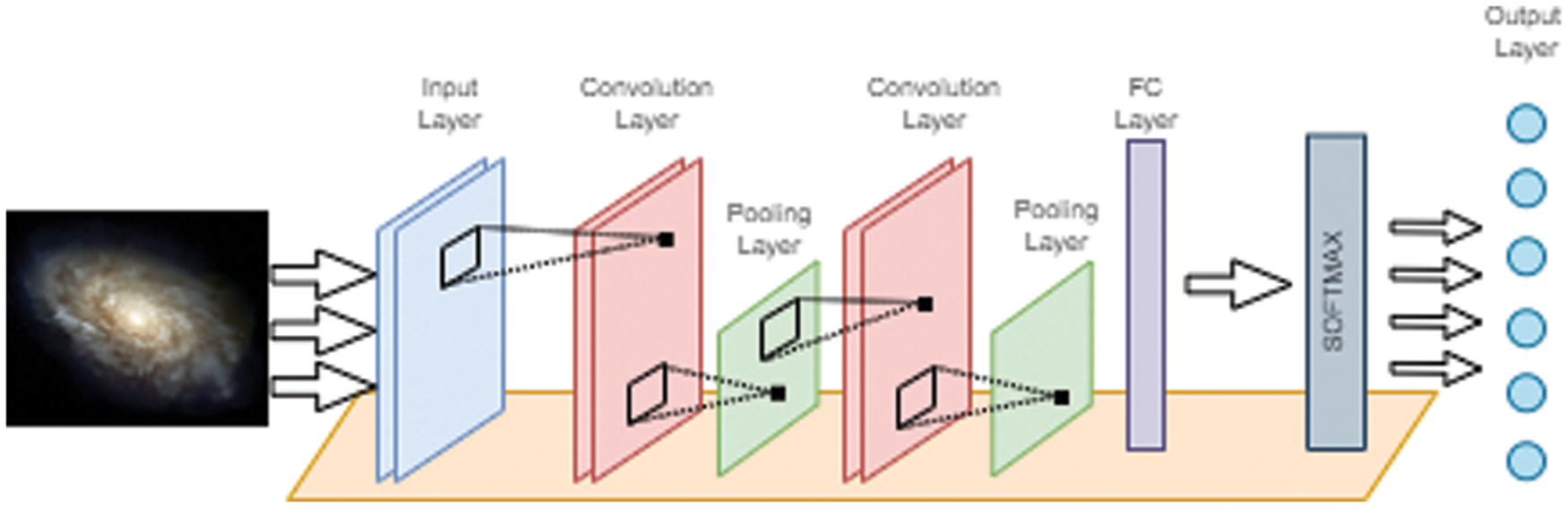
Figure 1: CNN architecture

The input layer is where the image data is applied raw to the CNN architecture. The input layer size is determined according to the resolution of the image. The convolution layer extracts the features from the images. In this layer, many features are obtained using filters of different sizes such as 2 × 2, 3 × 3, and 5 × 5. This filter is moved over all the pixels in order, starting from one corner of the picture. A new value is obtained by multiplying and summing the overlapping pixel values on the picture with the filter. In this way, different features are brought to the fore from each filter. Rectified Linear Unit (ReLu) activation function is generally used in the convolution layer.

The pooling layer is used to reduce the load on the hardware while working on the CNN architecture. It may cause some features to be lost but, it also prevents overfitting. It does not have to be used in every CNN architecture. All features extracted in the fully connected layer are smoothed into a single vector. Among the features extracted by this layer, the most contributing and non-contributing features to the classification are determined by updating the weights. The feature selection process is performed with this layer. In the SoftMax layer, the outputs of the FC layer are passed through the activation function and the class predictions are transferred to the output layer. The output layer predicts the class labels.

2.2 Grey Wolf Optimizer (GWO)

Grey Wolf Optimization (GWO) algorithm is a meta-heuristic optimization algorithm inspired by Grey wolves’ survival and hunting strategies in nature [31–33]. Grey wolves have a chain in which alpha wolves are at the top, and beta, delta, and omega wolves are listed, respectively (Fig. 2).

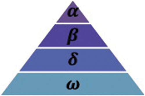
Figure 2: GWO algorithm hierarchy chain [31]

Alpha wolves represent the most dominant and commanding wolves, as seen from the chain structure. Beta wolves act as alpha wolves’ assistants and run the communication network between alpha wolves and other wolves. Omega wolves are the lowest level wolves chosen by alpha wolves. They are the ones who eat at last during hunting. Wolves that do not belong to the class of alpha, beta, or omega wolves are called delta wolves. Delta wolves are predominantly selected by alpha and beta wolves from omega wolves [34].

2.2.1 Hunting

Grey wolves hunt in the following three stages

•   Observing, tracking and approaching the prey

•   Encircling the prey and forcing it to move until it gets tired

•   Attacking the prey

In the GWO algorithm, alpha wolves represent the best solution. Beta and delta wolves represent the second and third best solutions, respectively. Finally, omega wolves represent candidate solutions.

D=|C∗Xp(t)−X(t)|(1)

X(t+1)=Xp(t)−A∗D(2)

Eqs. (1) and (2) in the GWO algorithm are used to express the encirclement of prey. It keeps the number of t instant iterations, Xp the position of the prey, X the position vector of a grey wolf. A and C represent the vector coefficients and are calculated as shown in Eqs. (3) and (4).

A=a∗(2∗r1−1)(3)

C=2∗r2(4)

Here, the random r1 and r2 are in the range of [0,1] and a denotes the linearly decreasing coefficient as the iteration progresses from 2 to 0.

2.2.2 Search

In GWO, the search process starts randomly, and the availability value of each wolf is calculated according to the cost function. The top three positions with the best availability value are represented as alpha, beta, and delta wolves, respectively. The alpha wolf coordinates the hunting process, and beta and delta wolves can join as needed. The positions of alpha, beta and delta wolves are updated as shown in Eqs. (5), (6), and (7).

Dα=|C1∗Xα−X(t)|Dβ=|C2∗Xβ−X(t)|Dδ=|C3∗Xδ−X(t)|(5)

Here, Xα, Xβ and Xδ represent the positions of alpha, beta, and delta wolves, respectively. The top three wolves are constantly updated in each iteration.

X1=|Xα−AαDα|X2=|Xβ−AβDβ|X3=|Xδ−AδDδ|(6)

X(t+1)=X1+X2+X33(7)

Here, X(t+1) denotes the new position of the prey.

2.2.3 Attack

After the location of the prey is determined in GWO, attacking the prey is carried out. Attacking the prey takes place after the prey gets tired and stops moving. Considering the mathematical modeling process, the attack process takes place according to the A value specified in Eq. (3). The A value is in [−2a,2a] and its value changes depending on the random variable r1. If the |A| value is greater than or equal to 1, Grey wolves will move away from the prey and start looking for a more suitable prey. If |A| is less than 1, the grey wolves are forced to attack the prey. This prevents getting blocked by local minimums. In GWO, the hunting process is continued until the stopping criterion is met or the specified number of iterations is reached.

3  Experimental Results

In this study, galaxy classification was made using the CNN method. Optimization of the CNN architecture with the support of the GWO algorithm has been carried out. In addition, a comparison was made with the Particle Swarm Optimization (PSO) [35] and Artificial Bee Colony (ABC) [36] algorithms, which are well known in the literature to compare the success of the GWO algorithm. The dataset and the CNN architecture used in the experimental studies are described in the following sections.

3.1 Dataset

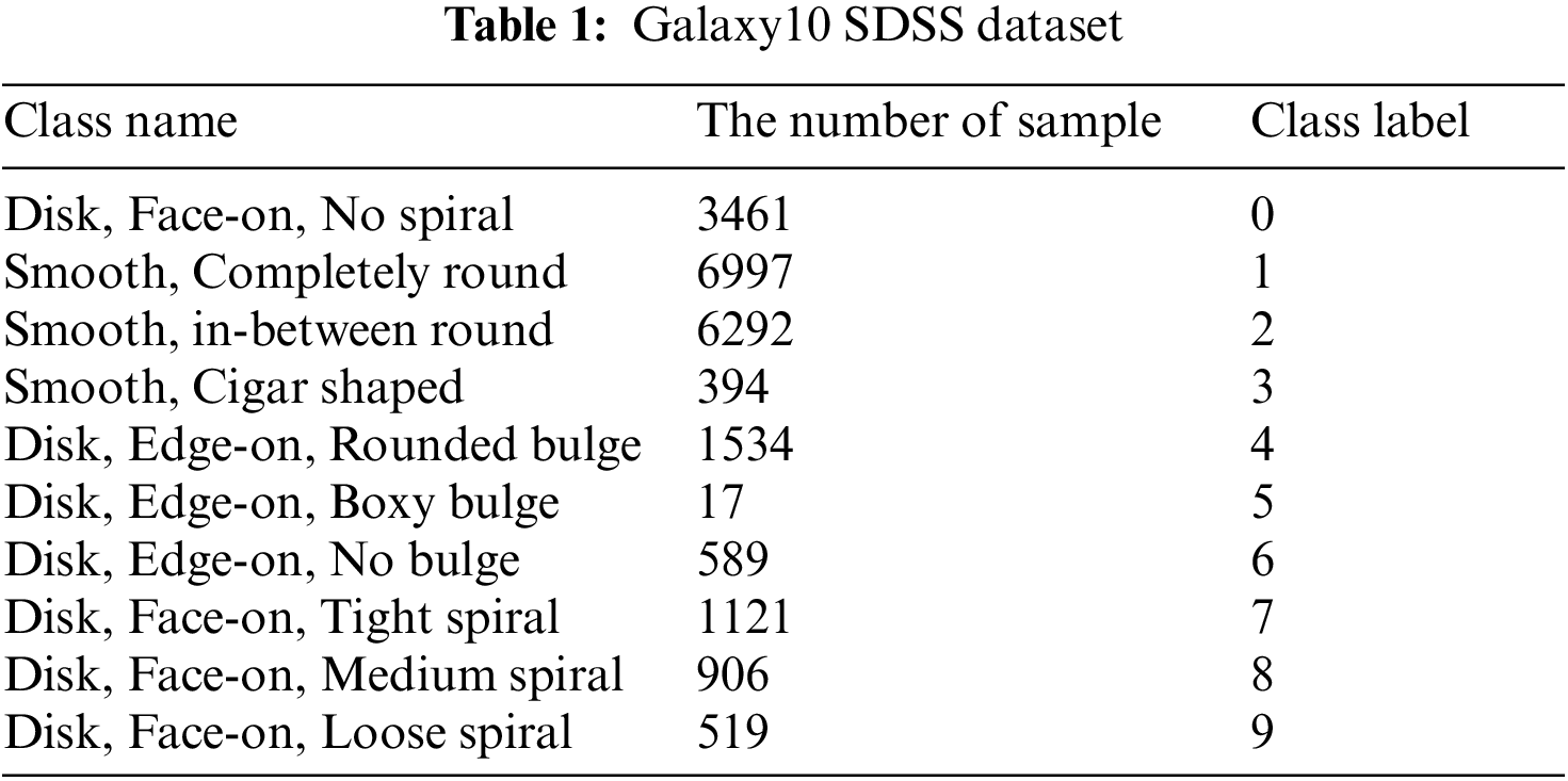
Galaxy images used in this study were created by Galaxy Zoo Project. Galaxy10 Sloan Digital Sky Survey (SDSS) Dataset [37] consists of ten classes, accepted by more than 55% of researchers. This dataset consists of 21785 images, that are 69 × 69 in size. Table 1 presents the classes of the dataset and the number of samples in each class.

In Fig. 3, sample images of the classes in the Galaxy10 SDSS dataset are shown. As seen from Fig. 3, there are 10 galaxy classes in the dataset. Although some classes are similar to each other, they differ from each other with small differences. These similar classes complicate the problem being considered. This situation requires a more complex CNN architecture instead of a simpler CNN architecture.

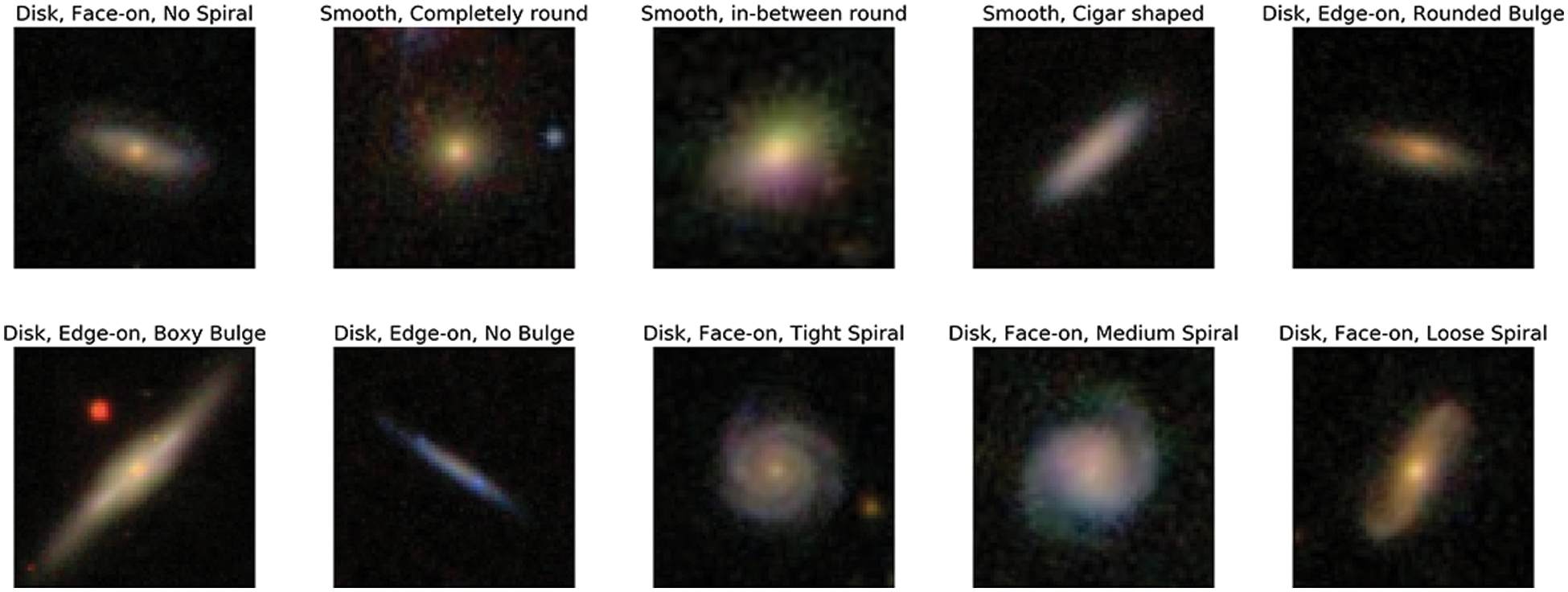
Figure 3: Example images of each class from the Galaxy10 dataset [37]

3.2 CNN Architecture

In this study, a basic CNN architecture was determined. The number of neurons in the layers of this architecture, learning coefficient and batch sizes were optimized. The CNN architecture is presented in Table 2, and ranges of optimized parameters are given in Table 3.

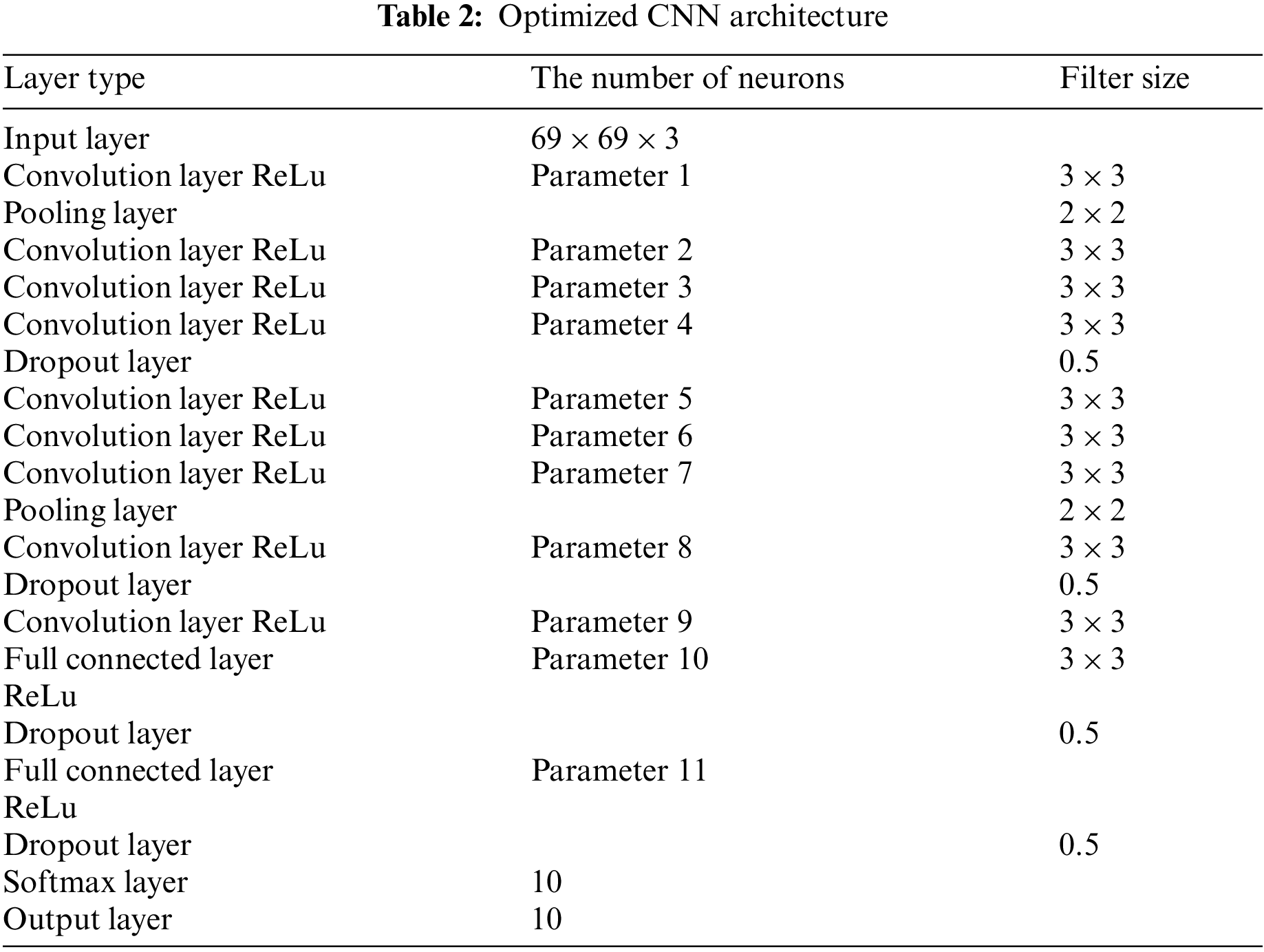
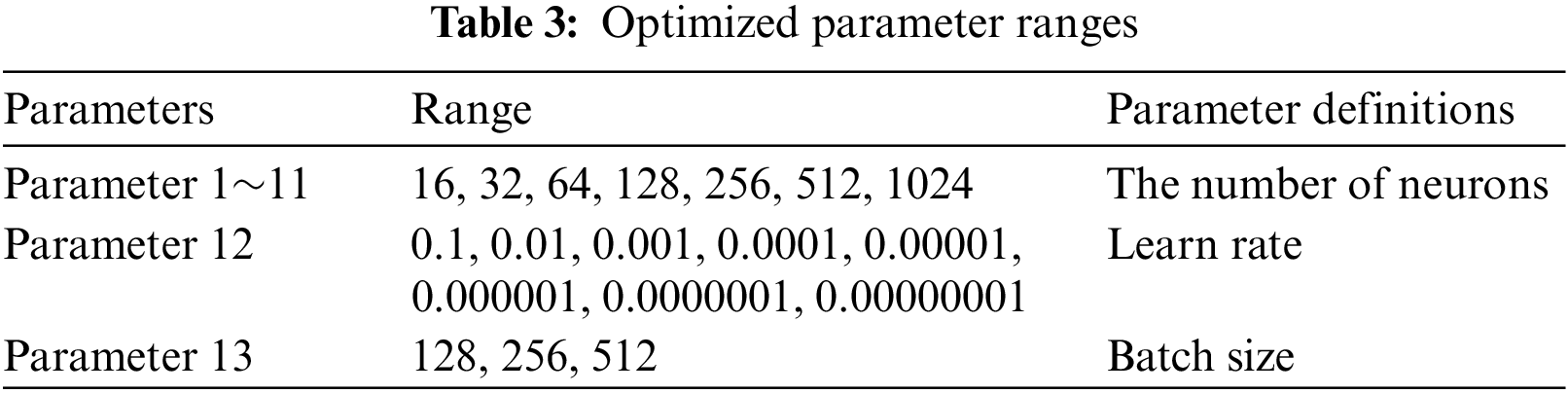
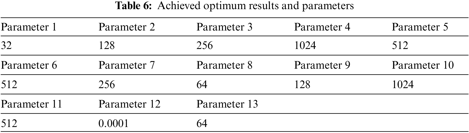
Parameter 1⁓11 given in Table 2 represents the number of neurons to be optimized. In addition to these parameters, Parameters 12 and 13 represent the learning coefficient and batch size, respectively.

3.3 Analysis

The parameters of the CNN architecture are optimized using the GWO algorithm. All operations have been carried out with Python 3.6 and Keras library. In the development of the CNN model, Adam optimizer as optimization function, Mean Squared Error (MSE) and Mean Absolute Error (MAE) as loss function, were used. MSE and MAE calculations are given in Eqs. (8) and (9), respectively. Fig. 4 shows the flow chart of the proposed method.

MSE=1n∑i=1n(yi−y~i)2(8)

MAE=1n∑i=1n|yi−y~i|(9)

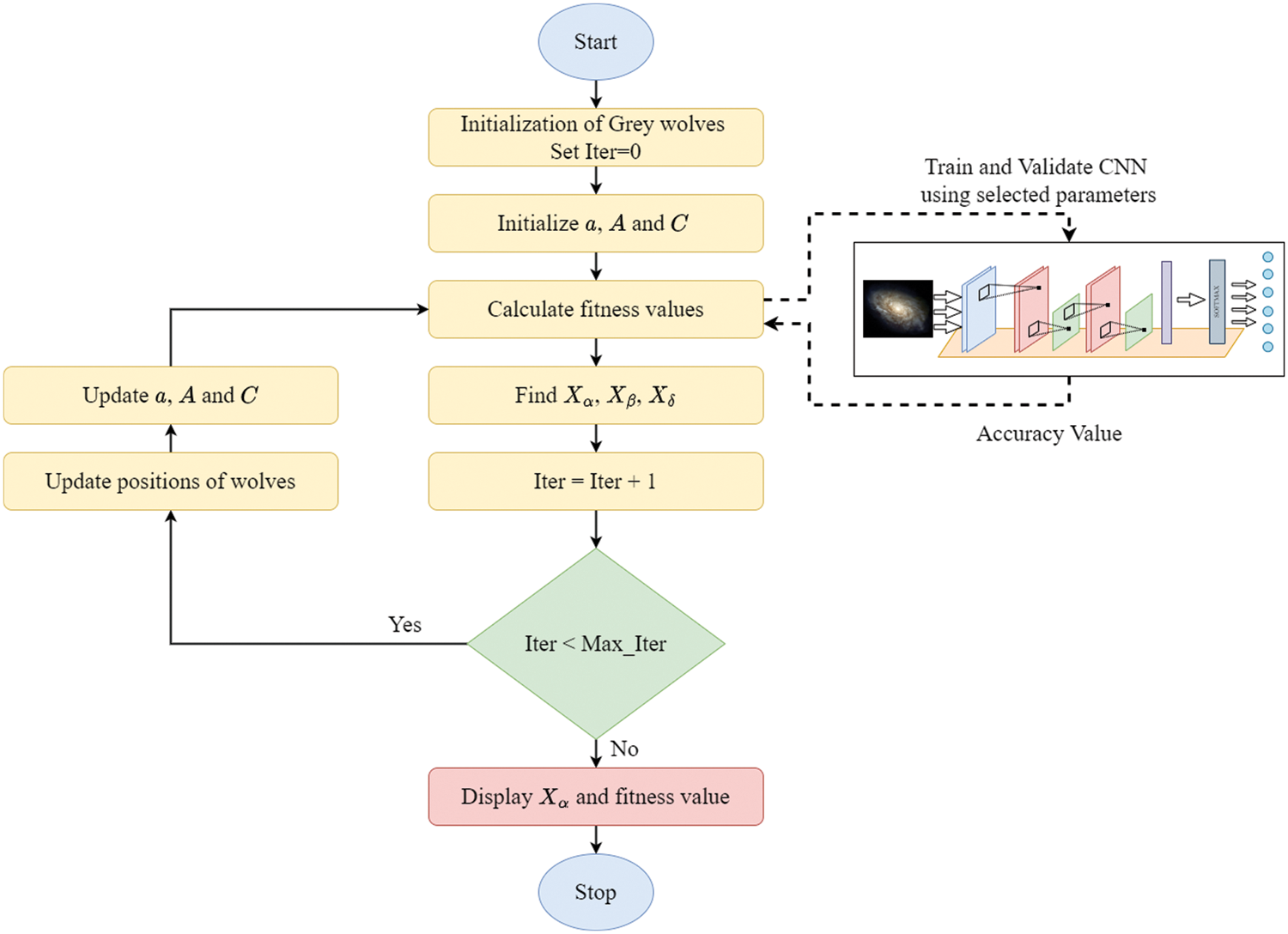
Figure 4: The flow chart of the proposed method

Here yi denotes the actual class label and y~i denotes the predicted class label.

In addition to the GWO algorithm, I optimized the CNN architecture with the well-known Particle Swarm Optimization (PSO) and Artificial Bee Colony (ABC) algorithms. These algorithms are used successfully in most real-world problems. The PSO and the ABC algorithms are state-of-art metaheuristic algorithms that were compared with GWO [38–43]. Therefore, these algorithms were used for comparison in this study.

The model’s accuracy value was considered as the cost function of the used metaheuristic algorithms. The accuracy formula is given in Eq. (10). It is aimed to determine the optimum parameters that will maximize the accuracy value.

Accuracy=NumberofCorrectPredictionsTotalNumberofPredictions(10)

A total of 21785 images were separated as training and test data with the 10-fold cross-validation technique. The optimum parameters of the CNN architecture were determined by metaheuristic algorithms. All algorithms were run with a population size of 30 and 50 iteration steps. In Table 4, the performance metrics of the train and test dataset are given. The best results were obtained with the GWO. To prevent overfitting in the CNN model, the training phase was terminated in cases where the dropout layers and early stop process and the validation accuracy value could not be improved for ten epochs. In addition, a comparison was made with another study using the same dataset in the literature [44]. The results of the reference study are presented in Table 4.

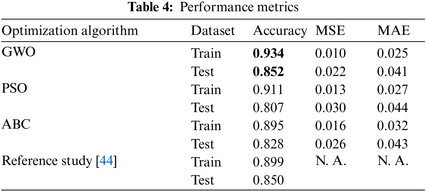
Considering the results given in Table 4, the test accuracy value was found to be 85%, whereas in the training as the accuracy was 93%. The GWO algorithm achieved better results than other metaheuristic algorithms. Compared to the Reference Study, the GWO algorithm is more successful in the training phase. In the test phase, the GWO algorithm achieved a better result by a small difference.

The differences between test and train results were examined, It was found that the model is not overfitting and performs a balanced learning process using GWO. During the model’s training, the accuracy and loss value of the model obtained with the train and test data are given graphically in Fig. 5 for the GWO.

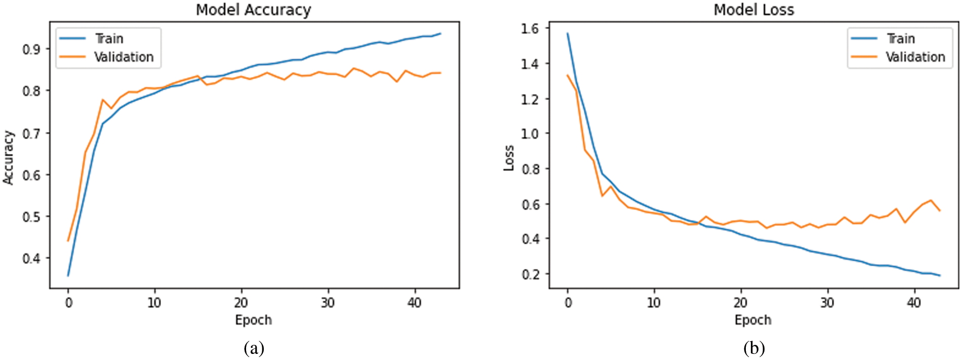
Figure 5: Development of accuracy and loss values during the training of the model (a) Accuracy graph (b) Loss value graph

The confusion matrix in Fig. 6 is given to see the classes that our model learned best and could not learn. A confusion matrix is a technique used to summarize the performance of a classification algorithm. If you have an unequal number of samples in each class, or more than two classes in your dataset, the classification accuracy alone can be misleading. A confusion matrix contains more detailed information about the classes in which your classification model fails. In this way, it can be easier to identify the areas to be focused on to improve the algorithm. The values in the matrix represent the classification results as percentages.

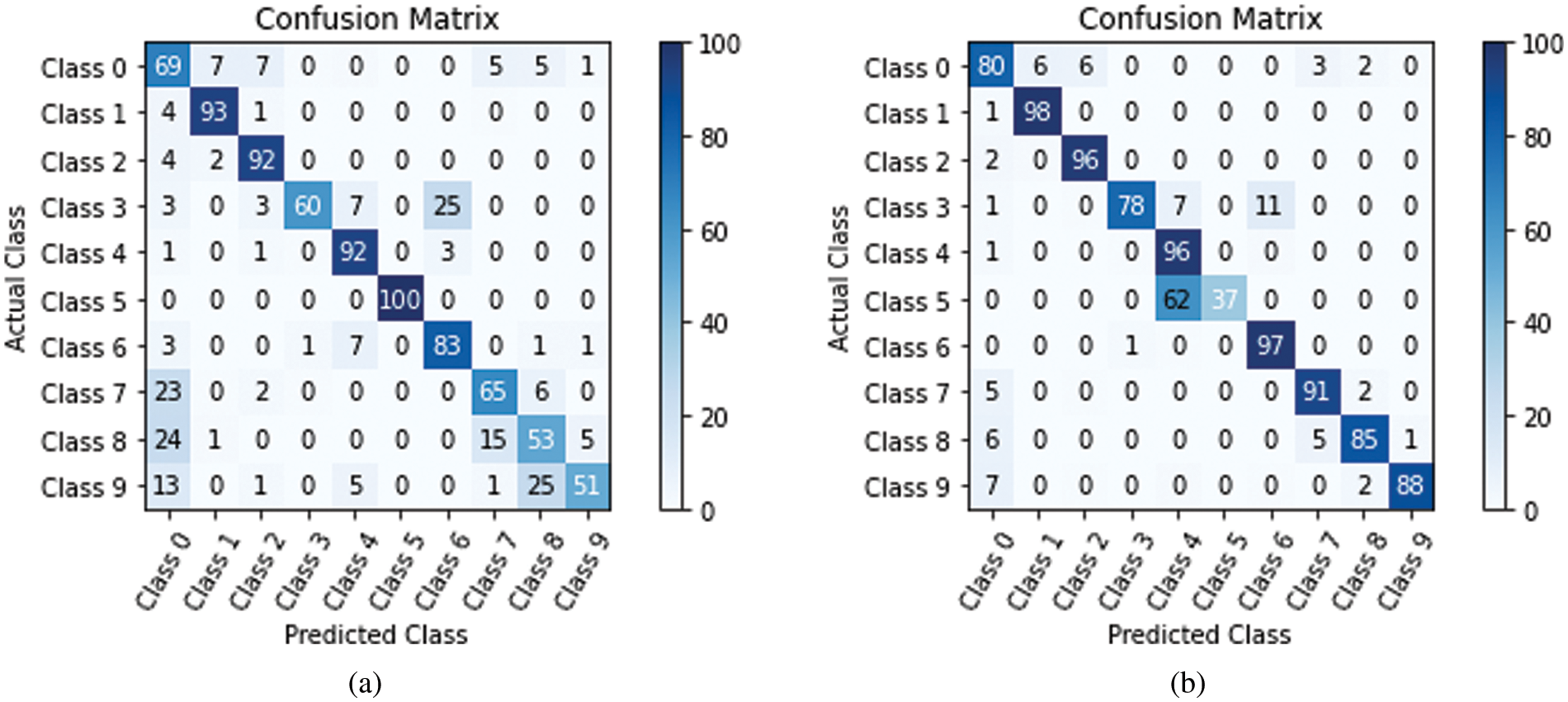
Figure 6: Confusion matrix of training and test dataset (a) Confusion matrix of test dataset (b) Confusion matrix of train dataset

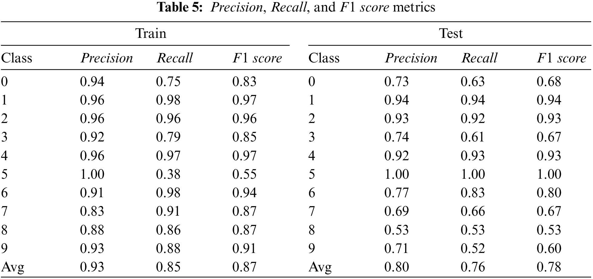
If Fig. 6 is examined, my model was able to learn Classes 1, 2, 4, 6 and 7 with an accuracy of over 90%. Except for Class 5, the remaining classes could be learned at a level considered successful. However, during the training phase, it learned very little about Class 5 and confused it with Class 4. As explained in the previous sections, our dataset has very little data belonging to Class 5. For this reason, the desired success in the learning process could not be achieved. Not including Class 5 in the study could have been considered as a solution, as there are very few examples compared to other class sample numbers. Since I assert a hybrid approach, I do not need to simplify my dataset. Learning achievements in the training phase are also seen in the testing phase. In direct proportion to the success in the training phase, classification was also possible in the testing phase. If the examples of all classes are examined in Fig. 3, it is understood that Classes 1 and 2 have a different and rounded shape from all other classes. Similarly, Classes 7 and 8 have a different spiral appearance than other classes. Galaxies belonging to the other six classes are in the form of disks and are likely to be confused with each other. The examples where the model will have the most difficulty learning are the examples of these six galaxy types. Based on the confusion matrix, the classes with the most success are Classes 1 and 2. Even though Class 8 has a helical appearance, it is a disc-like shape. For this reason, a classification as successful as the training results could not be obtained in the test results. In Class 4 and 6, my CNN model could generate a distinctive feature map and distinguish it from other disk-like galaxies. In Table 5, the Precision, Recall and F1Score values obtained by the GWO algorithm for each class are given. The data in Table 5 also supports the results in Fig. 6. The Precision, Recall and F1Score formulas are given in Eqs. (11), (12) and (13), respectively.

Precision=TPTP+FP(11)

Recall=TPTP+FN(12)

F1Score=2∗Precision∗RecallPrecision+Recall(13)

Here, TP, FP and FN represent True Positives, False Positives and False Negatives, respectively. As can be seen from Table 5, the small number of samples in Class 5 caused the Recall value to be low during training. Similarly, during the test, the Recall value of Classes 7, 8 and 9 is low. These classes have been mixed with other classes. This is clearly seen in the confusion matrix. In addition to Table 5, ROC curves of model results according to classes are given in Fig. 7.

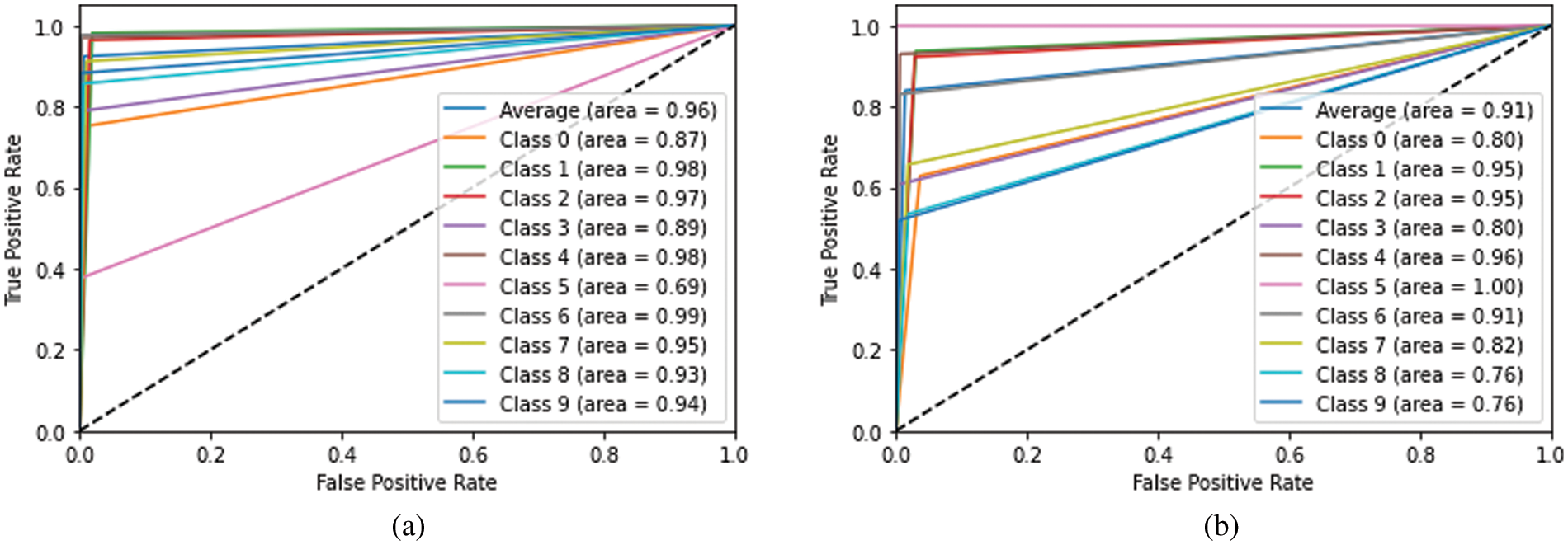
Figure 7: ROC curves of training and test dataset (a) Test dataset (b) Train dataset

In Table 6, the parameters of my optimally obtained CNN architecture are given. These parameters have been determined with the support of the GWO algorithm.

4  Conclusions

In this study, a morphological galaxy classification process was carried out. A hybrid approach is asserted using the Galaxy10 SDSS dataset. The neuron numbers, learning coefficient and batch size of the CNN architecture are adjusted with the help of meta-heuristic algorithms. The hyperparameter optimization process was calculated with the help of meta-heuristic algorithms. GWO, PSO and ABC algorithms, which are widely used in the literature, were selected. For an objective comparison, powerful state-of-the-art algorithm has been preferred. The learning process is difficult because the sample in the dataset is not homogeneously distributed. To overcome the problem, parameter adjustment is made with the help of an algorithm. The results show that the intended method can be used successfully in classification processes. Among the algorithms used, the GWO algorithm has been the most suitable for this problem. The GWO algorithm completed the training process with 93% accuracy and the testing process with 85% accuracy. Other algorithms have lagged this ratio. In future studies, a hybrid approach will be developed using homogeneous datasets.

Funding Statement: The author received no specific funding for this study.

Conflicts of Interest: The author declares that he has no conflicts of interest to report regarding the present study.

References

1. J. Stellato, “The Milky way and lentil beans,” Science Scope, vol. 43, no. 6, pp. 44–49, 2020. [Google Scholar]
2. L. Erlic, Galaxies, New York, USA: Weigl Publishers, 2019. [Google Scholar]
3. S. P. Driver, R. A. Windhorst and R. E. Griffiths, “The contribution of late-type/irregulars to the faint galaxy counts from HST medium deep survey images,” arXiv preprint astro-ph/9511123, 1995. [Google Scholar]
4. M. Rajesvari, A. Sinha, V. Saxena and S. A. Mukerji, “Deep learning approach to classify the galaxies for astronomy applications,” OSR-JEEE, vol. 15, pp. 35–39, 2020. [Google Scholar]
5. M. Reza, “Galaxy morphology classification using automated machine learning,” Astronomy and Computing, vol. 37, pp. 1–11, 2021. [Google Scholar]
6. D. Misra, S. N. Mohanty, M. Agarwal and S. K. Gupta, “Convoluted cosmos: Classifying galaxy images using deep learning,” in Advances in Intelligent Systems and Computing, vol. 1042, Singapore: Springer, pp. 569–579, 2020. [Google Scholar]
7. M. Biswas and R. Adlak, “Classification of galaxy morphologies using artificial neural network,” in 2018 4th Int. Conf. for Convergence in Technology (I2CT), Mangalore, India, pp. 1–4, 2018. [Google Scholar]
8. T. -Y. Cheng, C. J. Conselice, A. Aragón-Salamanca, N. Li, A. F. L. Bluck et al., “Optimizing automatic morphological classification of galaxies with machine learning and deep learning using dark energy survey imaging,” Monthly Notices of the Royal Astronomical Society, vol. 493, no. 3, pp. 4209–4228, 2020. [Google Scholar]
9. T. -Y. Cheng, C. J. Conselice, A. Aragón-Salamanca, M. Aguena, S. Allam et al., “Galaxy morphological classification catalogue of the dark energy survey year 3 data with convolutional neural networks,” Monthly Notices of the Royal Astronomical Society, vol. 507, no. 3, pp. 4425–4444, 2021. [Google Scholar]
10. A. Bastanfard, D. Amirkhani and M. Abbasiasl, “Automatic classification of galaxies based on SVM,” in 2019 9th Int. Conf. on Computer and Knowledge Engineering (ICCKE), Mashhad, Iran, pp. 32–39, 2019. [Google Scholar]
11. L. M. Goyal, M. Arora, T. Pandey and M. Mittal, “Morphological classification of galaxies using conv-nets,” Earth Science Informatics, vol. 13, no. 4, pp. 1427–1436, 2020. [Google Scholar]
12. M. Abd Elaziz, K. M. Hosny and I. M. Selim, “Galaxies image classification using artificial bee colony based on orthogonal Gegenbauer moments,” Soft Computing, vol. 23, no. 19, pp. 9573–9583, 2019. [Google Scholar]
13. K. Kayaalp and S. Metlek, “Classification of robust and rotten apples by deep learning algorithm,” Sakarya University Journal of Computer and Information Sciences, vol. 3, no. 2, pp. 112–120, 2020. [Google Scholar]
14. K. Kayaalp and S. Metlek, “Prediction of fish species with deep learning,” International Journal of 3D Printing Technologies and Digital Industry, vol. 5, no. 3, pp. 569–576, 2021. [Google Scholar]
15. R. Vidhya and T. T. Mirnalinee, “Hybrid optimized learning for lung cancer classification,” Intelligent Automation & Soft Computing, vol. 34, no. 2, pp. 911–925, 2022. [Google Scholar]
16. A. Aleem, S. Tehsin, S. Kausar and A. Jameel, “Target classification of marine debris using deep learning,” Intelligent Automation & Soft Computing, vol. 32, no. 1, pp. 73–85, 2021. [Google Scholar]
17. H. S. Gill, O. I. Khalaf, Y. Alotaibi, S. Alghamdi and F. Alassery, “Fruit image classification using deep learning,” Computers, Materials & Continua, vol. 71, no. 3, pp. 5135–5150, 2022. [Google Scholar]
18. R. Thamizhamuthu and D. Manjula, “Skin melanoma classification system using deep learning,” Computers, Materials & Continua, vol. 68, no. 1, pp. 1147–1160, 2021. [Google Scholar]
19. I. M. Nasir, M. A. Khan, M. Alhaisoni, T. Saba, A. Rehman et al., “A hybrid deep learning architecture for the classification of superhero fashion products: An application for medical-tech classification,” Computer Modeling in Engineering & Sciences, vol. 124, no. 3, pp. 1017–1033, 2020. [Google Scholar]
20. B. Barman, R. K. Dewang and A. Mewada, “Facial recognition using grey wolf optimization,” Materials Today: Proceedings, vol. 58, no. 1, pp. 273–285, 2022. [Google Scholar]
21. T. Muto and M. Maeda, “Grey wolf optimization with momentum for function optimization,” Artificial Life and Robotics, vol. 26, no. 3, pp. 304–311, 2021. [Google Scholar]
22. Q. Fan, H. Huang, Y. Li, Z. Han, Y. Hu et al., “Beetle antenna strategy based grey wolf optimization,” Expert Systems with Applications, vol. 165, pp. 1–19, 2021. [Google Scholar]
23. K. Shahverdi and J. M. Maestre, “Gray wolf optimization for scheduling irrigation water,” Journal of Irrigation and Drainage Engineering, vol. 148, no. 7, pp. 1–9, 2022. [Google Scholar]
24. F. A. Şenel, F. Gökçe, A. S. Yüksel and T. Yiğit, “A novel hybrid PSO–GWO algorithm for optimization problems,” Engineering with Computers, vol. 35, no. 4, pp. 1359–1373, 2019. [Google Scholar]
25. E. S. El-Kenawy and M. Eid, “Hybrid gray wolf and particle swarm optimization for feature selection,” International Journal of Innovative Computing, Information and Control, vol. 16, no. 3, pp. 831–844, 2020. [Google Scholar]
26. P. M. Kitonyi and D. R. Segera, “Hybrid gradient descent grey wolf optimizer for optimal feature selection,” BioMed Research International, vol. 2021, pp. 1–33, 2021. [Google Scholar]
27. R. Al-Wajih, S. J. Abdulkadir, N. Aziz, Q. Al-Tashi and N. Talpur, “Hybrid binary grey wolf with harris hawks optimizer for feature selection,” IEEE Access, vol. 9, pp. 31662–31677, 2021. [Google Scholar]
28. D. Wei, J. Wang, Z. Li and R. Wang, “Wind power curve modeling with hybrid copula and grey wolf optimization,” IEEE Transactions on Sustainable Energy, vol. 13, no. 1, pp. 265–276, 2022. [Google Scholar]
29. Z. H. Yue, S. Zhang and W. D. Xiao, “A novel hybrid algorithm based on grey wolf optimizer and fireworks algorithm,” Sensors (Switzerland), vol. 20, no. 7, pp. 1–17, 2020. [Google Scholar]
30. X. P. Zhu, J. M. Dai, C. J. Bian, Y. Chen, S. Chen et al., “Galaxy morphology classification with deep convolutional neural networks,” Astrophysics and Space Science, vol. 364, no. 4, pp. 1–15, 2019. [Google Scholar]
31. S. Mirjalili, S. M. Mirjalili and A. Lewis, “Grey wolf optimizer,” Advances in Engineering Software, vol. 69, pp. 46–61, 2014. [Google Scholar]
32. X. Song, L. Tang, S. Zhao, X. Zhang, L. Li et al., “Grey Wolf Optimizer for parameter estimation in surface waves,” Soil Dynamics and Earthquake Engineering, vol. 75, pp. 147–157, 2015. [Google Scholar]
33. S. Mirjalili, “How effective is the grey wolf optimizer in training multi-layer perceptrons,” Applied Intelligence, vol. 43, no. 1, pp. 150–161, 2015. [Google Scholar]
34. A. Tunç, “Using machine learning techniques of detect the credit availability for the financial sector,” M.S. Thesis, Computer Enginnering, Selçuk University, Konya, Turkey, Country, 2016. [Google Scholar]
35. J. Kennedy and R. Eberhart, “Particle swarm optimization,” in Proc. of ICNN’95-Int. Conf. on Neural Networks, Perth, WA, Australia, pp. 1942–1948, 1995. [Google Scholar]
36. D. Karaboga and B. Basturk, “A powerful and efficient algorithm for numerical function optimization: Artificial bee colony (ABC) algorithm,” Journal of Global Optimization, vol. 39, no. 3, pp. 459–471, 2007. [Google Scholar]
37. H. Leung and J. Bovy, “Galaxy10 SDSS dataset—astroNN 1.1.dev0 documentation,” 2022. https://astronn.readthedocs.io/en/latest/galaxy10sdss.html (accessed on 17 March 2022). [Google Scholar]
38. A. K. Tripathi, K. Sharma and M. Bala, “A novel clustering method using enhanced grey wolf optimizer and MapReduce,” Big Data Research, vol. 14, pp. 93–100, 2018. [Google Scholar]
39. C. Lu, L. Gao, X. Li, C. Hu, X. Yan et al., “Chaotic-based grey wolf optimizer for numerical and engineering optimization problems,” Memetic Computing, vol. 12, no. 4, pp. 371–398, 2020. [Google Scholar]
40. S. Gottam, S. J. Nanda and R. K. Maddila, “A CNN-LSTM model trained with grey wolf optimizer for prediction of household power consumption,” in Proc.-2021 IEEE Int. Symp. on Smart Electronic Systems, iSES 2021, MNIT Jaipur, Rajasthan, India, pp. 355–360, 2021. [Google Scholar]
41. K. Tütüncü, M. A. Şahman and E. Tuşat, “A hybrid binary grey wolf optimizer for selection and reduction of reference points with extreme learning machine approach on local GNSS/leveling geoid determination,” Applied Soft Computing, vol. 108, pp. 1–13, 2021. [Google Scholar]
42. R. Akbari and M. R. Hessami-Kermani, “Parameter estimation of muskingum model using grey wolf optimizer algorithm,” MethodsX, vol. 8, pp. 1–15, 2021. [Google Scholar]
43. B. N. Gohil and D. R. Patel, “Load balancing in cloud using improved gray wolf optimizer,” Concurrency and Computation: Practice and Experience, vol. 34, no. 11, pp. 1–13, 2022. [Google Scholar]
44. A. Nandan and V. Tripathi, “Galaxy shape categorization using convolutional neural network approach,” in 2022 IEEE 11th Int. Conf. on Communication Systems and Network Technologies (CSNT), Indore, India, pp. 287–293, 2022. [Google Scholar]
Cite This Article
Copyright © 2023 The Author(s). Published by Tech Science Press.
This work is licensed under a Creative Commons Attribution 4.0 International License , which permits unrestricted use, distribution, and reproduction in any medium, provided the original work is properly cited.
Downloads
Citation Tools