Efficient Gait Analysis Using Deep Learning Techniques

1  Introduction

Recognizing daily routine-based on human activities such as walking, standing, sitting, etc., could be a difficult statistical task to classify them and draw some inferences from them. It involves anticipating a person’s movement based on sensor [1] data, and it typically required deep domain expertise and signal processing methodologies to correctly create features from the data to suit a machine learning model [2]. Deep learning approaches such as Convolution Neural Networks (CNN) and Recurrent Neural Networks have recently demonstrated that they are capable of learning features from raw sensor data and can even attain state-of-the-art outcomes.

Recognizing daily routine based on human activities has a major role to play in the case of interpersonal relations and human-to-human interaction. It is difficult to extract them as it provides information about a person identification, personality, and condition. One of the most considered subjects in the scientific fields of computer vision and machine learning is the human ability to recognize another person’s activity. Many applications such as video surveillance systems, human-computer interaction, and robotics for human behavior characterization require a multiple activity recognition systems as a result of this research. Recognition of these human activities aims to classify or categorize someone’s actions based on a sequence of sensor readings. Adults with Cerebral Palsy (CP) have a variety of persistent movement abnormalities that impede body and muscle coordination and are caused by injury to one or more parts of the brain at the moment of their birth. Roughly two-thirds of people with Cerebral Palsy (CP) can walk on their own, while the majority of them have diplegia or spastic hemiplegia. To enhance gait ability in people with CP, multidisciplinary techniques involving numerous therapies such as orthotics, physical therapy, orthopedic surgery, and chemical neurolysis are used. One of the primary objectives of these techniques is to identify the appropriate suggestions and increase the efficacy of the treatments [3]. Despite the need for impartial data to study the result of the therapies, gait assessment in practice generally depend on intuitive visual examination and clinical examination by therapists rather than a systematic review of Spatio-temporal gait parameters [4]. It owes to the scarcity of comprehensive gait examination that necessitates specialized laboratory investigations involving complicated technologies like Optical Motion Capture which comes with the significant expense and time constraints [5–9].

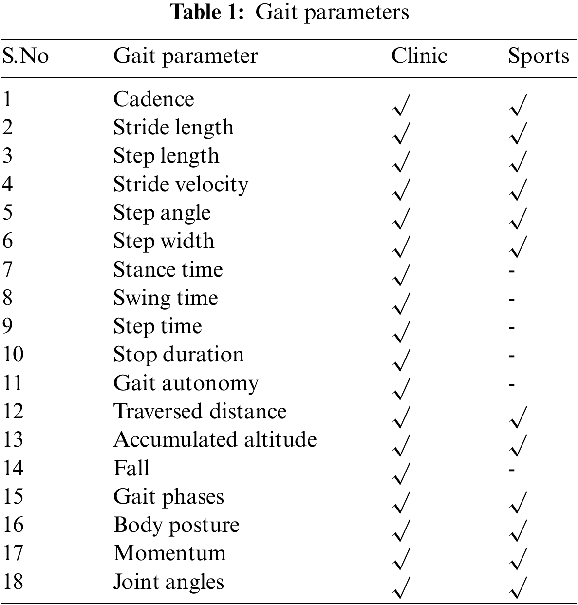
Notably, a wearable smart system that relies on accelerometers, gyroscopes, and a specific algorithm for consistent, efficient measurement of spatiotemporal gait parameters in older adults [10] and Parkinson’s disease patients [11] was developed and verified for gait analysis. The method is centered on the observation of gyro gestures, where the algorithm detects temporal parameters and analyzes gait aspects outside of a laboratory context using the 3D foot trajectory. Data extraction and analysis can be done quickly and easily with the use of specialized algorithms, resulting in a quick and easy-to-understand output that does not require the heavy setup and technical skills required by a comprehensive 3D gait laboratory [12]. The different parameters of gait and its applications are given in the Table 1.

2  Related Studies

Gait analysis is essential in a wide range of Child Protective Services (CPS) applications, including patient response, movement disorder prediction, athletic evaluation, fault diagnosis, and a slew of other immersive virtual reality applications. As a result, current research has concentrated on employing wearable sensors to measure step duration, a critical metric in gait analysis. Several pieces of research based on the gait analysis are given below.

Rosquist et al. [13] have confirmed the application of accelerometer sensors on the low trunks, utilizing camera footage and peer distance as a representational method. Cutler et al. [14] stressed the importance of obtaining at minimum an aggregate of 4 consecutive steps in Gross Motor Function Classification System (GMFCS) I kids, and at minimum six sequential strides in Gross Motor Function Classification System Expanded and Revised (GFMCS) II and III kids, to allow a meaningful estimate of gait characteristics. Zihajehzadeh et al. [15] offer a biophysical framework that uses knee flexion into consideration and estimates step length and gait disproportionateness using data from 4 less power consumable Inertial Measurement Units (IMU) mounted on legs. With a 4.9 cm Root Mean Square Error (RMSE), the presented dual pendulum method predicted the step length. The model treats the hips as a singular pivot joint, neglecting the pelvis joints’ displacement in the course of movements, resulting in step length estimate inaccuracies. Wu et al. use an inverse kinematics model with 3.69% MAPE to estimate step length by connecting 2 Inertial Measurement Unit (IMU) dev-kits here on patients’ feet. Ankle and pelvic girdle aren’t taken into account in their model. Instead, it uses motion sensors attached to the ankle to determine the length of the step based on the limb measurement and the slope of the leg’s alignment.

Grad et al. [16] use accelerometers in cell phones to capture motion data and design an app to do so. They also employ an inverse kinematics model to predict step length with a Mean Absolute Percentage Error (MAPE) of less than 10%. Neither of these researches assesses stride length or gait velocity, two more important parameters for gait function research. Using four high-cost Ultra Wide Band (UWB) range sensing with four IMUs on the rear and front of each feet, a recent study tackles the limitations of prior experiments [17]. It uses a geometric trapezoidal proximity model to estimate step length with a Root Mean Square Error (RMSE) of 4.1 cm and a Mean Absolute Percentage Error (MAPE) of 4.75 percent. The high computation demands of the info from 8 sensors, on the other hand, enhance the system’s complexity and power consumption. 2 IMUs (Inertial Measurement Unit) are placed on the foot, 2 IMUs (Inertial Measurement Unit) are placed on the stiles, two IMUs are placed on the thigh, and 1 IMU is placed on the hips in a recent study [18].

3  Architecture of Human Activity Recognition

The main objective of this project is to identify the best neural network model which can help in the human activity recognition process. The features which are provided as an input to the neural network model have a much higher influence on the model from a performance point of view. Generating features from a huge amount of raw data is a very crucial step in machine learning or deep learning models to solve any classification challenge. Features help to express the useful properties of unprocessed data in such a way that the user can understand and can be used by the neural network or any non-neural network model for that matter. These features which are interpretations of original data are critical in improving the model’s performance. As a result, the goal of the research is to find a superior set of feature combinations [19].

The architecture of the whole approach is given in the figure given below. The main modules of our system include exploratory data analysis, data pre-processing, and human activity recognition using classification. The primary objective of this whole setup is to choose the finest neural network model for the recognition of human activity [20]. As far as the initial step of our human activity recognition analysis is concerned, the values of acceleration along all the three axes-X axis, Y axis, and Z axis fed into our neural network model are taken from the Wireless Sensor Data Mining (WISDM) lab dataset given in their website. The second step is to do exploratory data analysis which includes exploring the content of all variables and analyzing each of them with the required plots for each of them. The next step is to clean and pre-process the raw time series data that has been obtained [21]. Once the data pre-processing has been completed, acceleration values can be provided as input to the neural network classification algorithms to categorize the activities into walking, running, upstairs, downstairs, sitting, and standing.

3.1 Dataset

The dataset contains data collected through controlled laboratory conditions [22]. It is raw time series data taken from WISDM (Wireless Sensor Data Mining) lab’s website. Dataset consists of 1,098,207 examples and 6 attributes like walking, running, upstairs, downstairs, sitting, and standing. As far as the class distribution is concerned these are the highest number of samples for walking [23] (4,24,400 which is almost 38.4% of our total samples) and the lowest number of samples for standing (48,395 which is equal to 4.4% of our total samples). Raw data is imbalanced and so data balancing is done in the data pre-processing section.

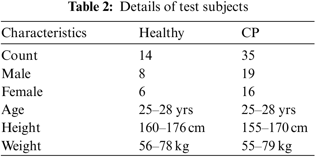
For examining cerebral palsy (CP) nearly 1490 gait cycles were examined in total and are useful for the comparison. The average accuracy ± precision for stride length, cadence, and step length was 3.5 ± 4.3, 4.1 ± 3.8, and 0.6 ± 2.7 cm respectively. Elaborative details on the test subjects are given in Table 2.

3.2 Exploratory Data Analysis

In this work, six activities have been taken into consideration-walking, running, upstairs, downstairs, sitting, and standing. These activities are chosen since many people perform regularly in their daily activities or routine. In addition to this, most of these activities include repetitive movements and this also makes the tasks easier to detect. When this data was recorded in the WISDM lab, for each of these activities acceleration was recorded on three axes X-axis, Y-axis, and Z-axis. So in this case the X-axis corresponds to the user’s leg moving horizontally, Y-axis refers to the user’s upward and downward movements and Z-axis finally refers to the user’s leg moving forward.

Fig. 1 depicts all the plots of accelerometer data for an individual, for all three axes, and each of the six activities and Fig. 2 shows the number of examples corresponding to each human activity.

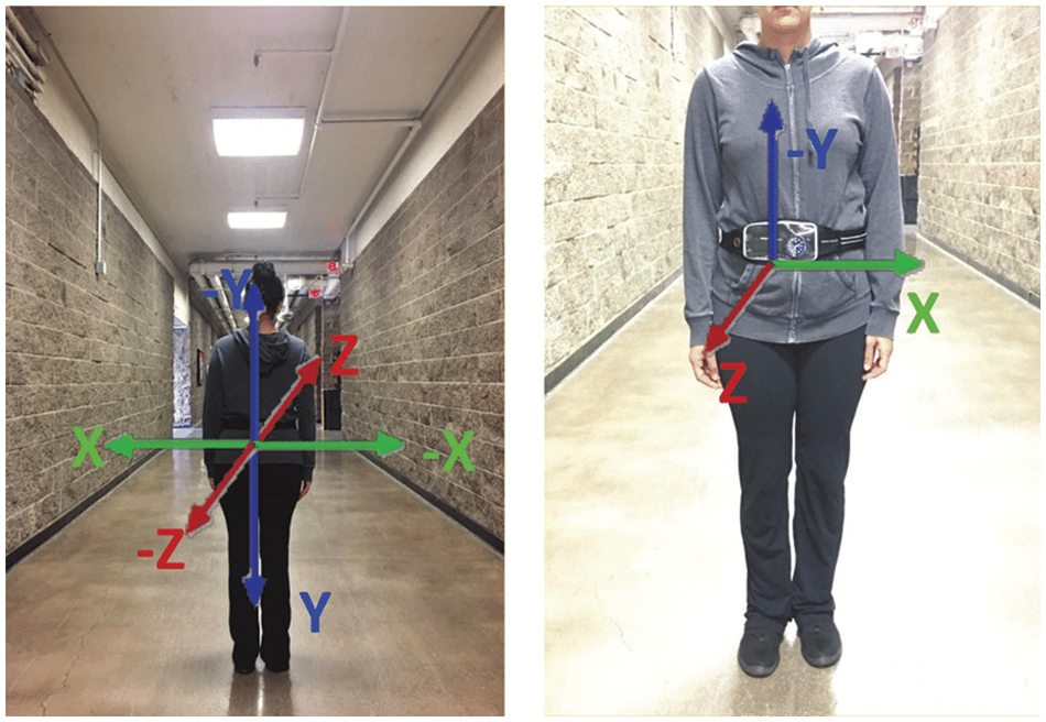
Figure 1: Shows all three different axes from an individual’s point of view

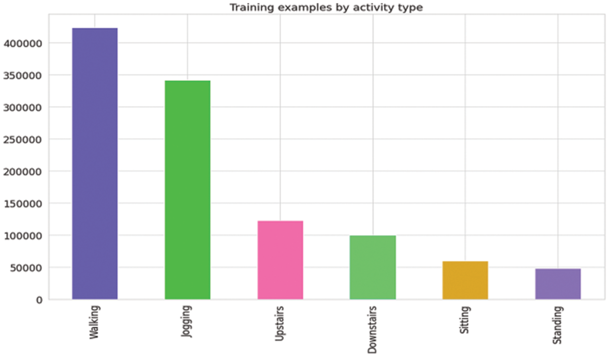
Figure 2: Just shows the number of examples corresponding to each human activity

The training data for the x, y, and z axes recorded by the accelerometer for the sitting posture is shown in the Fig. 3 below. As far as the x-plot is concerned, the plot remains steady and comparable to the plot of standing classes [24]. The data plotted for sitting is nearly identical to that plotted for standing on the y-axis, with the exception that it is slightly steadier [25]. In the case of z-axis, it appears by distinguishing between standing and sitting is troublesome because the user does not exert a lot of movement on the mobile device in the two conditions.

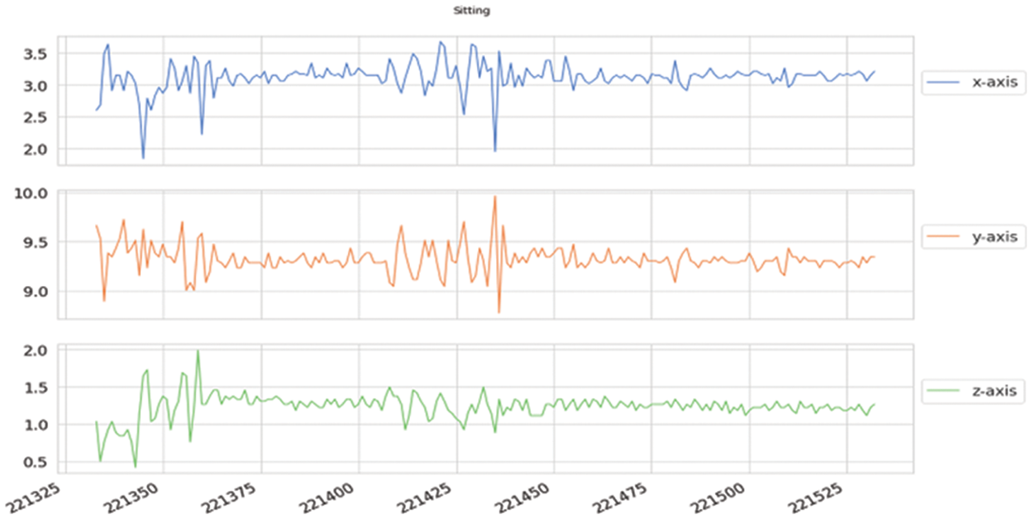
Figure 3: The training data for the x, y, and z axes recorded by the accelerometer for the sitting posture

The training for the coordinate axes for the standing class recorded by the accelerometer is shown in Fig. 4 below. Because there is essentially no motion, the x-axis is quite steady near the zero mark. Because of the continuous gravity attraction, the y-axis is relatively steady at around 9.8 m/s2, and the z-axis is quite similar to the walking graph, but without the constant peaks created by the gadget moving to and fro in a direction opposite to the screen [26].

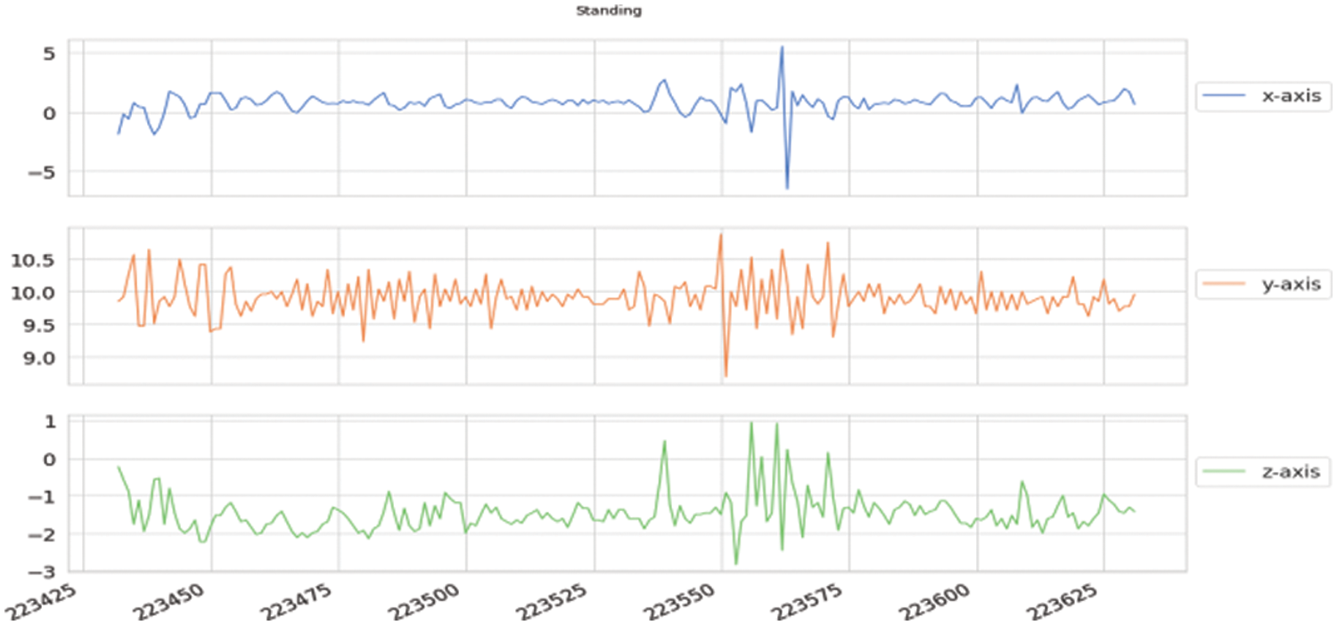
Figure 4: Training for the coordinate axes for the standing class recorded by the accelerometer

The data accessible for the walking data class is represented in Fig. 5 below on the x, y, and z-axes, respectively. Each of the three axes’ peaks is roughly the same distance apart, but all of them have their intensity and range.

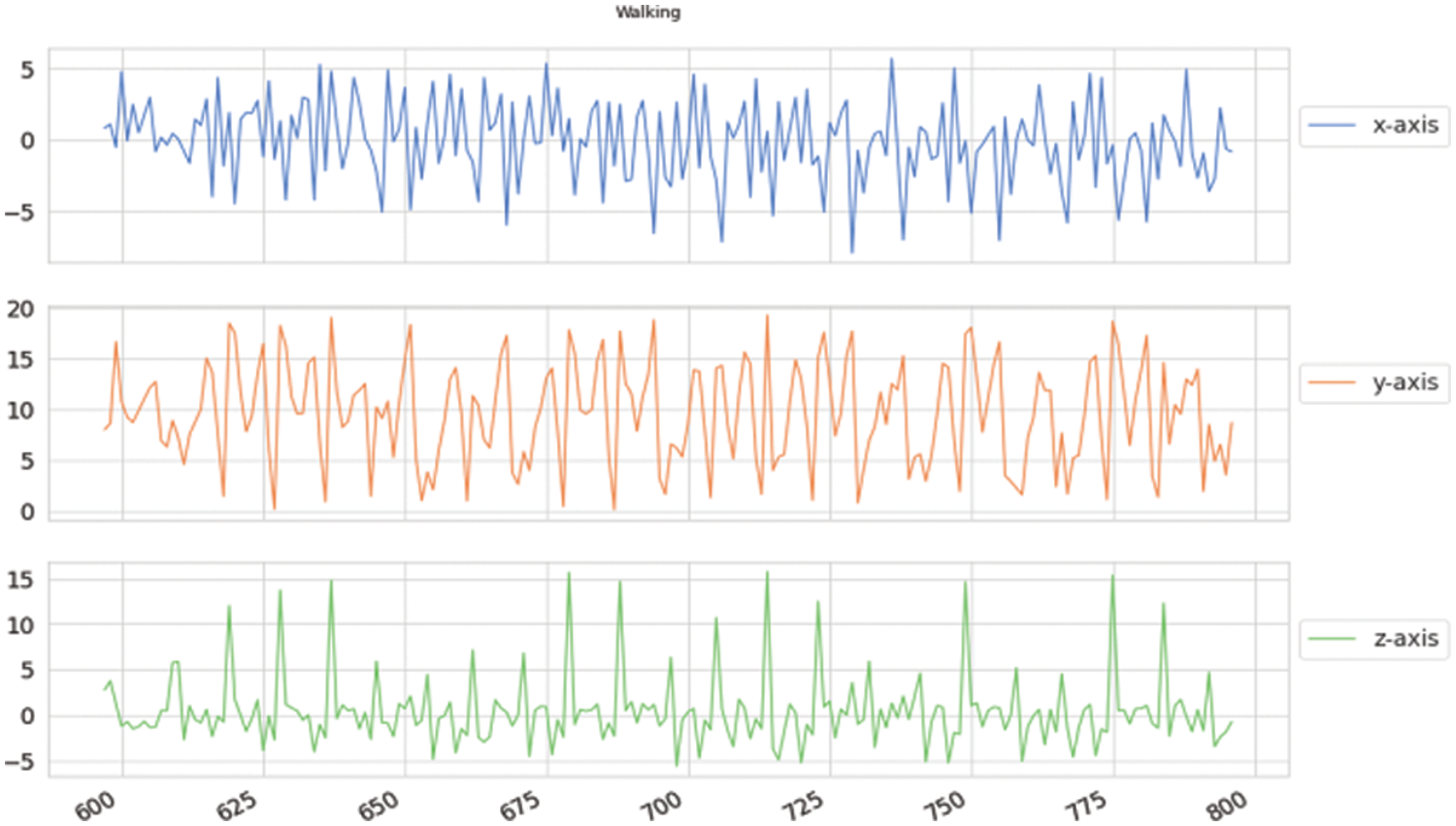
Figure 5: Data accessible for the walking data class

The training data for the x, y, and z axes for the jogging category is shown in Fig. 6, and downstairs data is shown in Fig. 7. The x-axis data differentiates itself from those of the other categories, with values ranging from −10 to 10, unlike the other classes. In general, the time between peaks is shorter than that of activities like walking. Except for the correlation with the walking group, where the two of them swing from 0 to 20, the y-axis data in the picture below is highly noticeable when compared to other classes.

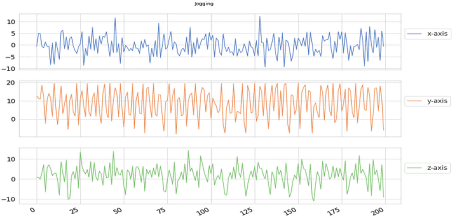
Figure 6: Data accessible for the Jogging class

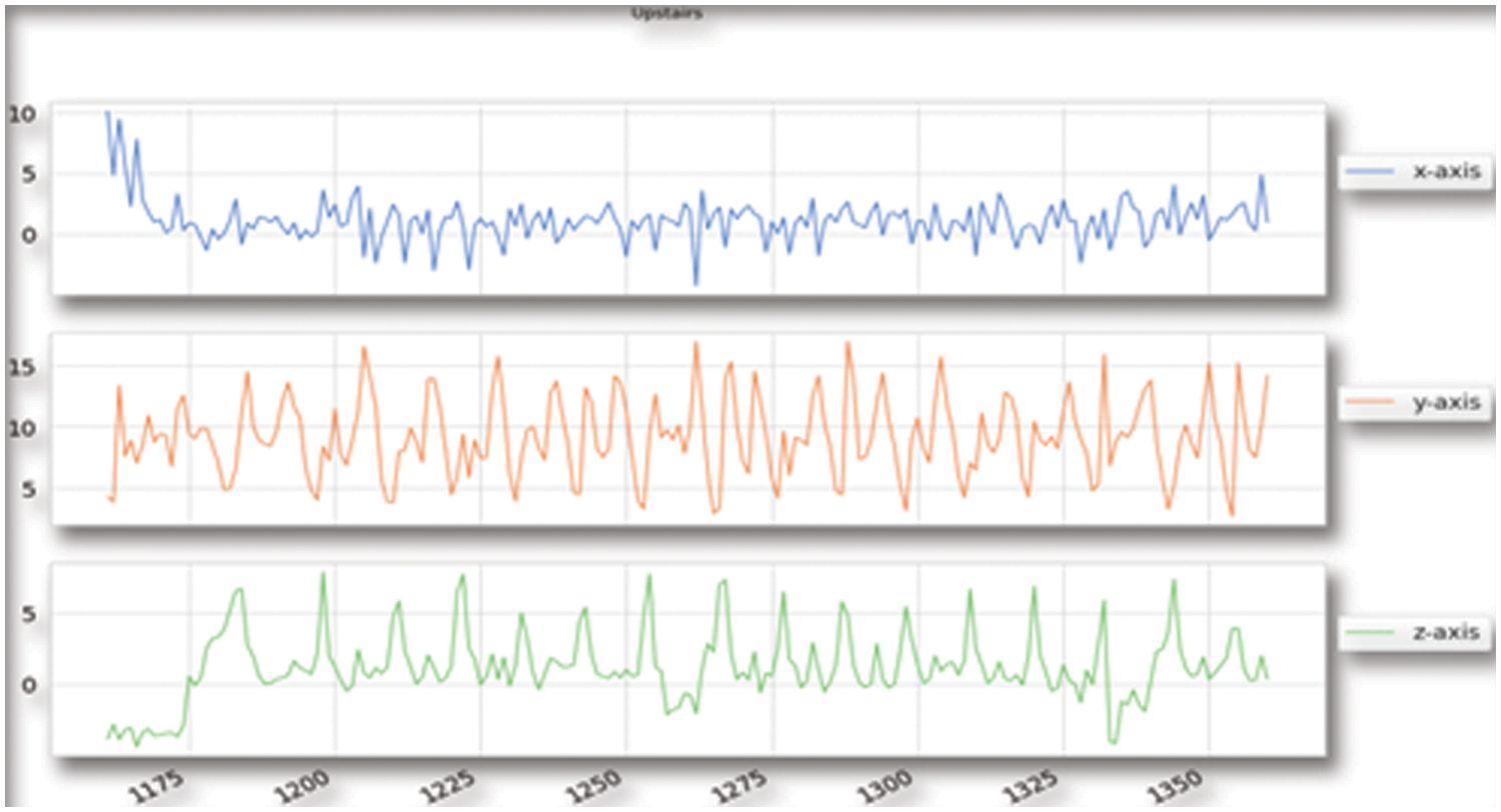
Figure 7: Graphs for the downstairs data

3.3 Data Pre-Processing

To apply standard neural network classification algorithms, raw time series data must be transformed according to the way inputs are fed into the network. Basic data pre-processing is done initially which is applicable for any model for that matter such as data balancing so that model is not biased towards any particular output which is the human activity in our case. Apart from that, Label Encoding is a must as it helps in translating the labels to a numeric format to make them machine-readable [27].

The next step is to do pre-processing according to the neural network model being used, so there are certain factors that need to be considered before that as it is a time series data, the sampling rate given is equal to 20 Hz which means one sample every 50 ms. While feeding inputs to our neural network model, the step value is chosen as 20.

The final step of our data pre-processing step before starting to create the model is to split the data into 4:1 ratio, i.e., use 80% for training the data and 20% for testing our data. Any train-test split with more data in the training set will almost certainly result in improved accuracy on the test set. So, the one training the model can make it 70:30 or 75:25 depending on him/her, it would still give them better accuracy.

3.4 Validation

Gyroscope units that analyze the 3D foot trajectory for Spatio-temporal gait examination have been validated with standard optoelectronic gesture capture systems with worthy accuracy in healthy individuals and CP disease patients. The deviation for ankle dorsiflexion was corrected using the minimum velocity updates during the stance phase. This was achievable because each subject could place the whole plantar surface of their shoe on the surface during the load and push stages of stance. This is the first study within our insight that has validated an accelerometer sensor against a 3D gait evaluation standard in people with CP, displaying high accuracy, precision, and agreement. The system received favorable reviews from all of our participants, who found it to be light and simple to ignore when walking. To determine to what extent such parameters influence walking kinematics, formal investigations examining gait parameters with and without wearable devices, and also outdoors and inside laboratory settings, are needed.

4  Methodology

4.1 2D CNN Model

In most existing work, 1D convolution is applied to single univariate time series, whereas multi-sensors or multi-modality results in multivariate time series. So, the 2D CNN model is used when applied to multivariate time series, 2D convolution and pooling operations capture local dependency in both the temporal and spatial domains for unimodal data, resulting in higher performance with fewer parameters than 1D operation [28].

Spatial reliance across sensors, as well as regional dependency over the long run, is both very important for obtaining distinct features from numerous sensors. However, employing a CNN with a 1D convolution kernel and a 1D pooling kernel, each signal’s local reliance over time is simply captured. So, proposed CNN with a 2D convolution kernel and a 2D pooling kernel to capture both types of dependency (Figs. 8 and 9). Two kinds of modalities are managed when using multiple sensors: sensors in different places and diverse sensor types [29–32]. For each sort of modality, considered simple pre-processing and aggregated the inputs from multiple sensors in different poses to capture structural dependency between them. Because various types of sensors, such as accelerometers, gyroscopes, and magnetometers, have distinct attributes, applying convolution kernels to them without separating them might make it difficult to extract fresh characteristics. To avert this, differentiate different sensors by padding zeros between them in the first convolutional layer so that they do not end up in the same convolution kernel.

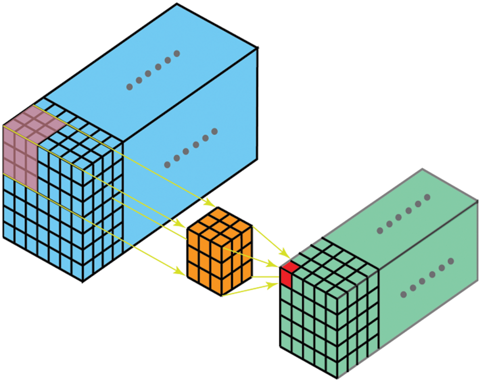
Figure 8: Types of kernels

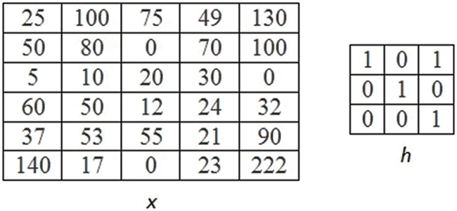
Figure 9: Input image X and kernel h

The 2D convolution on the kth feature map’s position (i, j) in the lst layer is:

zi,jl,k=∑k′=1K′∑x=1X∑y=1Ywx,y,k′l−1,k(1)

where the size of the convolution kernel over signals and overtime are X and Y respectively, at (l – 1)th layer, number of feature maps is denoted by K` and a convolution kernel which is formed by the weight tensor is w^l−1, k′ ∈ R^ (X × Y × K′).

The 2D pooling on the kth feature map’s position (i, j) in lth layer is:

zi,jl,k=σ(.⋯.⋮maxzi′,j′l−1,k.(i−1)P+1≤i′P,(j−1)Q+1≤j′Q,.)(2)

where the activation function is σ (⋅) and P * Q is the size of the pooling layer.

Fig. 10 depicts the overall CNN structure employed in this work. One input layer, two convolutional layers, two sub-sampling layers, and two fully linked layers make up the seven layers. The following common deep learning approaches are used to produce more accurate activity identification systems. Rectified Linear Unit (ReLU) is used as the activation function to avoid overfitting.

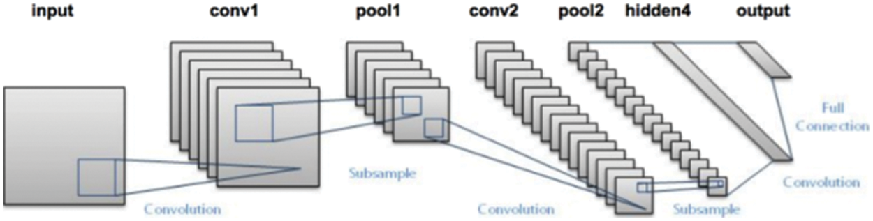
Figure 10: Overall CNN model

The equation of the ReLU function is given below:

f(x)=max(0,x)(3)

The vanishing gradient problem, which occurs when error falls exponentially to zero during error propagation between layers, plagued gradient-based learning techniques with different forms of activation functions, such as sigmoid. Because the gradient value is in the range [0, 1], the error decreases exponentially when the gradient values are multiplied layer by layer. Whereas, the gradient value of ReLU can only have two values, 0 and 1:

f′(x)=1 whenx>0,0x≤0(4)

As a result, using ReLU (Rectified Linear Unit) as an activation function does not make the issue go away. Furthermore, since the gradient value will be 1 or 0, propagation calculation is made considerably easier.

At the last layer, the Softmax function is utilized to categorize each signal into one of the N activity types. N nodes are inserted in this layer, which is equal to the number of activity classes. The value of N in our situation is 6. The Softmax function at each node ensures that the output value is in the range [0, 1] and that the sum is one:

Softmax(zj)=exp⁡(zj)∑n=1Nexp⁡(zn),forj=1,…,N(5)

The likelihood that the test signal belongs to activity class j is then equivalent to softmax as a result of CNN’s output (zj).

4.2 LSTM Model

Long Short Term Memory (LSTM) network models are a sort of recurrent neural network that are ready to recall and learn long sequences of facts that are provided as input. They are designed to work with data that consists of long sequences of data with up to 400-time steps. The advantage of utilizing LSTMs for sequence classification is that they learn directly from raw statistical data, eliminating the need for domain expertise to manually build input features. The model should be able to learn an indoor representation of the statistical data and, in theory, perform similarly to models trained on a version of the dataset with artificial features [33–35].

Training LSTMs removes the matter of Vanishing Gradient (weights become too small that under-fits the model), but it still faces the difficulty of Exploding Gradient (weights become large that over-fits the model).

As far as the architecture of the model is concerned, LSTMs shown in Fig. 6 is dealing with both Long Term Memory (LTM) and Short-Term Memory (STM), and the concept of gates is used to make the calculations simple and effective.

1.    Forget Gate: When LTM enters the forget gate, it discards information that is no longer helpful.

2.    Learn Gate: The event (current input) and the STM are merged so that the relevant information from the STM is applied to this input.

3.    Remember Gate: In Remember Gate LTM information that hasn’t been forgotten with STM and Event information to create an updated LTM is combined.

4.    Use Gate: This gate predicts the output of this event using LTM, STM, and Event, and acts as an updated STM.

The actual mathematical architecture of the LSTM is represented using the following Fig. 11 below.

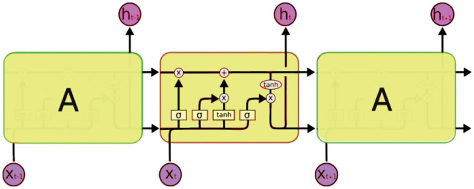
Figure 11: Actual mathematical architecture of LSTM model

4.3 Bi-LSTM Model

Bi-LSTM RNN (Recurrent Neural Network) architecture has been selected because it is believed that this model is better suited for recognizing daily routine human activities. Sequence input, Bidirectional long short-term memory (Bi-LSTM) layer, long short-term memory (LSTM), fully connected, softmax, and classification) layers were used in our Bi-LSTM RNN (Recurrent Neural Network) design.

The complete architecture of our whole Bi-LSTM model is shown in Fig. 12 below.

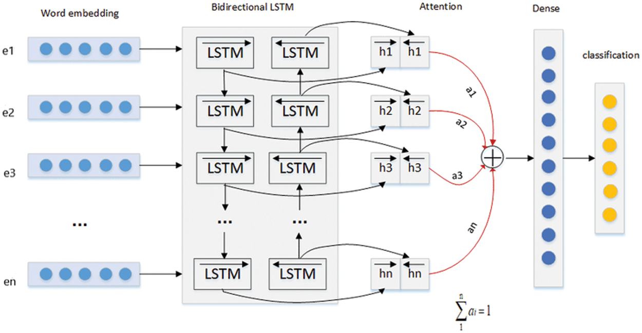
Figure 12: Whole architecture of Bi-LSTM model

In total, 17 layers are there in the input sequence. With 150 hidden units and 201,600 parameters, the output of layer Bi-LSTM equals 300. The output of the LSTM layer is 150, with 150 hidden units and 270,600 parameters. Because there are six classes in the WISDM lab dataset, the fully connected network has 150 and 6 as input size and output size respectively.

The validation subset was used to assess the design’s correctness and stop training accordingly, and the testing subset to compare the design’s performance to that of others while avoiding bias. The number of layers was determined by various trial and error techniques to maximize the model’s performance and get the best possible accuracy.

Cadence (steps per minute), Gait cycle duration (s), swing as well as stance ratio, and double-support were used in this study; stance was separated into 3 stages: foot flat, load, and push [36–38]. Speed (m/s), Stride length (m), toe clearance (m), and maximal heel, turning angle and angular velocity were the spatial parameters. Gait analysis using these characteristics has previously been reported and validated in both young and old people. Here it is calculated foot angle at starting and ending contact to evaluate individual CP gait symptoms. Because CP gait shall be defined by the initial and terminal contact, toe-striking terms were used over the typical toe-off and heel-strike definitions.

Strike anglen=θ(ticn)(6)

Angle of take-offn=θ(ttcn)(7)

where Strike angle and Angle of take-off were calculated for individual gait cycle (n), using the foot angular position along its pitch axis (u), as well as the period of preliminary and final contact. Fig. 13 below shows the visualization of the same.

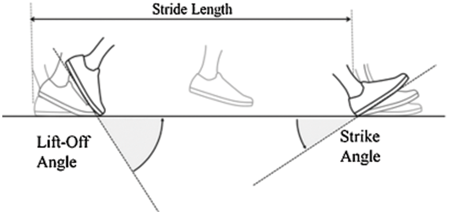
Figure 13: Calculation of stride length

4.4 Experiment

In the gait laboratory, all the participants were instructed to reiterate the small walking trials, along with a 10 m straightforward walk test. Subjects were instructed to walk 300 meters at their own pace across a long and wide hallway to evaluate the measuring gadget in a true clinical setting. The 300-meter exam consisted of three 100-meter straight walks separated by 180° twists. Gait cycles that turned were automatically discovered and removed from the analysis. The coefficient of variability was used to assess inter-stride variability (CV).

5  Experimental Evaluation

Evaluating the performance of learning systems plays a vital role in any classification problem statement. The majority of learning algorithms are built to predict the class of “future” unlabelled data items. In some circumstances, testing hypotheses is a necessary step in the learning process (In the case of machine learning when pruning a decision tree).

5.1 Neural Network Models Employed

Three neural network models are employed for the analysis of human activities which need to be recognized–the 2D Convolution neural networks (CNN) model, long short-term memory (LSTM) model, and the bi-directional LSTM model. The reason for choosing the 2D CNN model is that it uses a hierarchical model that builds a network, similar to a funnel, and then outputs a fully-connected layer where all the neurons are connected and the output is processed. The reason for working with LSTM and Bi-LSTM is that they can capture long-term dependencies between word sequences and hence are better used for classification. Generally, Models based on Bi-LSTM (Bidirectional long-short-term memory) provide better predictions than models based on LSTM alone. In particular, it was discovered that Bi-LSTM models outperform ARIMA (An Auto-Regressive Integrated Moving Average) and LSTM (long short-term-memory model) in terms of prediction.

A learning curve can be defined as a graphical representation of the link between how proficient someone is at a task and also the amount of experience they need. In our case, the learning curve of the model indicates that the model is neither over-fitted nor under-fitted as shown in Figs. 14–17 for loss and accuracy respectively.

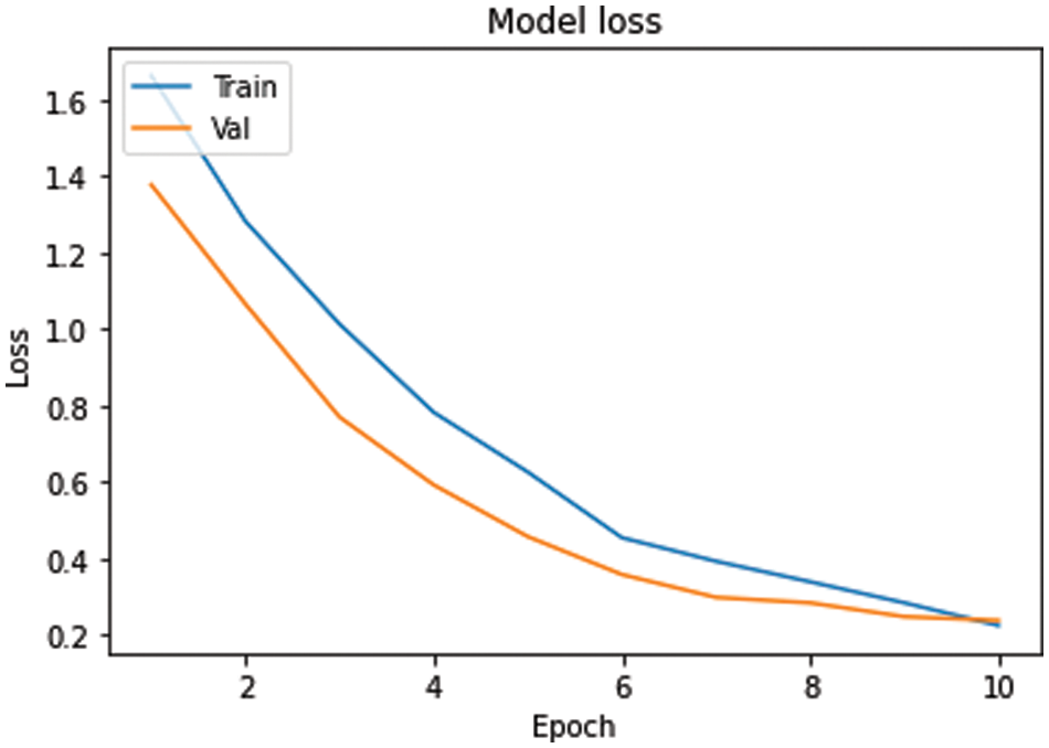
Figure 14: Loss of 2D CNN model

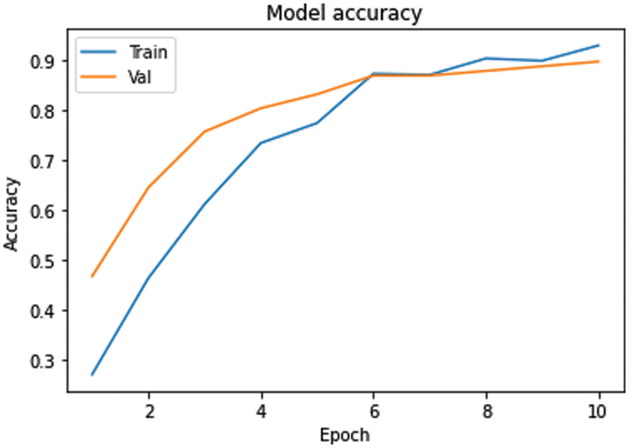
Figure 15: Accuracy of 2D CNN model

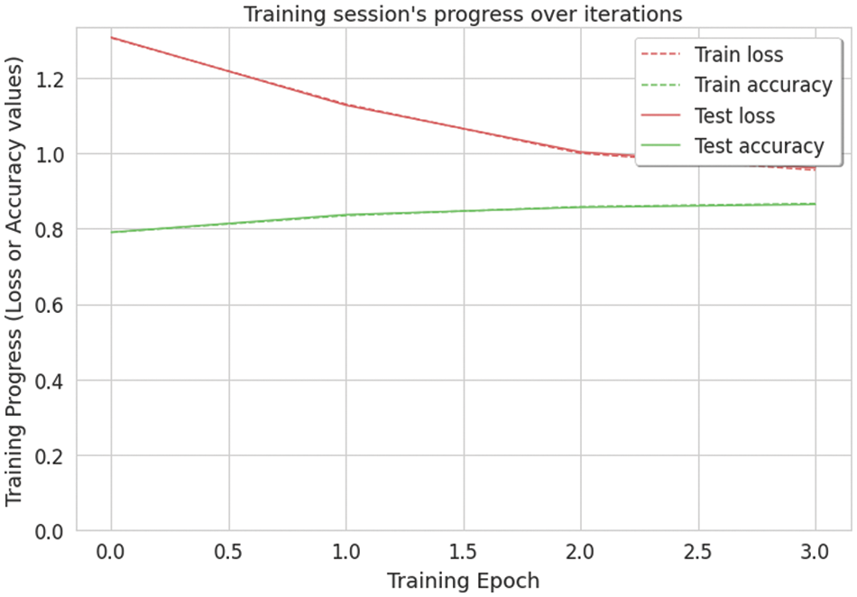
Figure 16: Loss and accuracy of the LSTM model

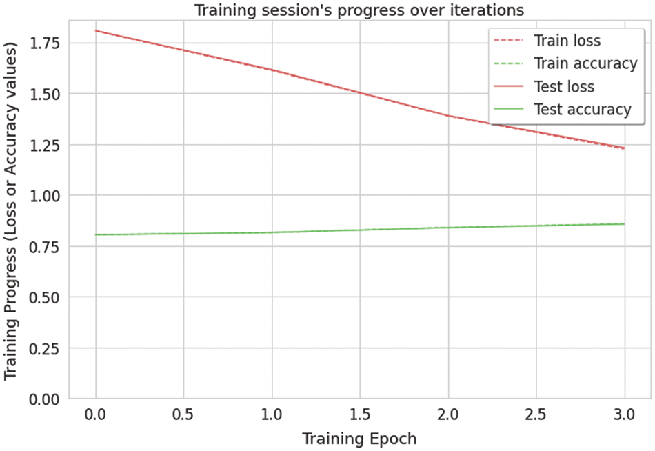
Figure 17: Loss and accuracy of Bi-LSTM model

A confusion matrix can be defined as a table used to describe the performance of a classification model (or “classifier”) on a set of test data for which the correct values or outputs are known. Well, it is a performance measurement for any machine learning or deep learning classification problem statement for that matter where the output can be two or more classes. In this case, 6 classes were used-walking, running, upstairs, downstairs, sitting, and standing. It’s great for determining Recall, Precision, Specificity, Accuracy, and, most importantly, the AUC (Area under Curve)–ROC (Receiver Operating Characteristic Curve) Curve. The confusion matrix of all three models is shown below in Figs. 18–20.

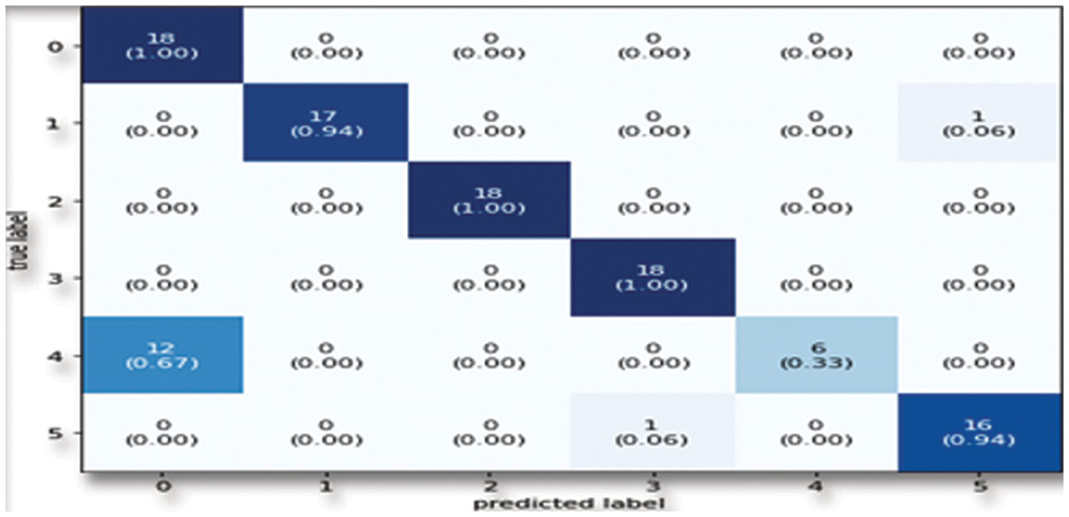
Figure 18: Confusion matrix for 2D CNN model

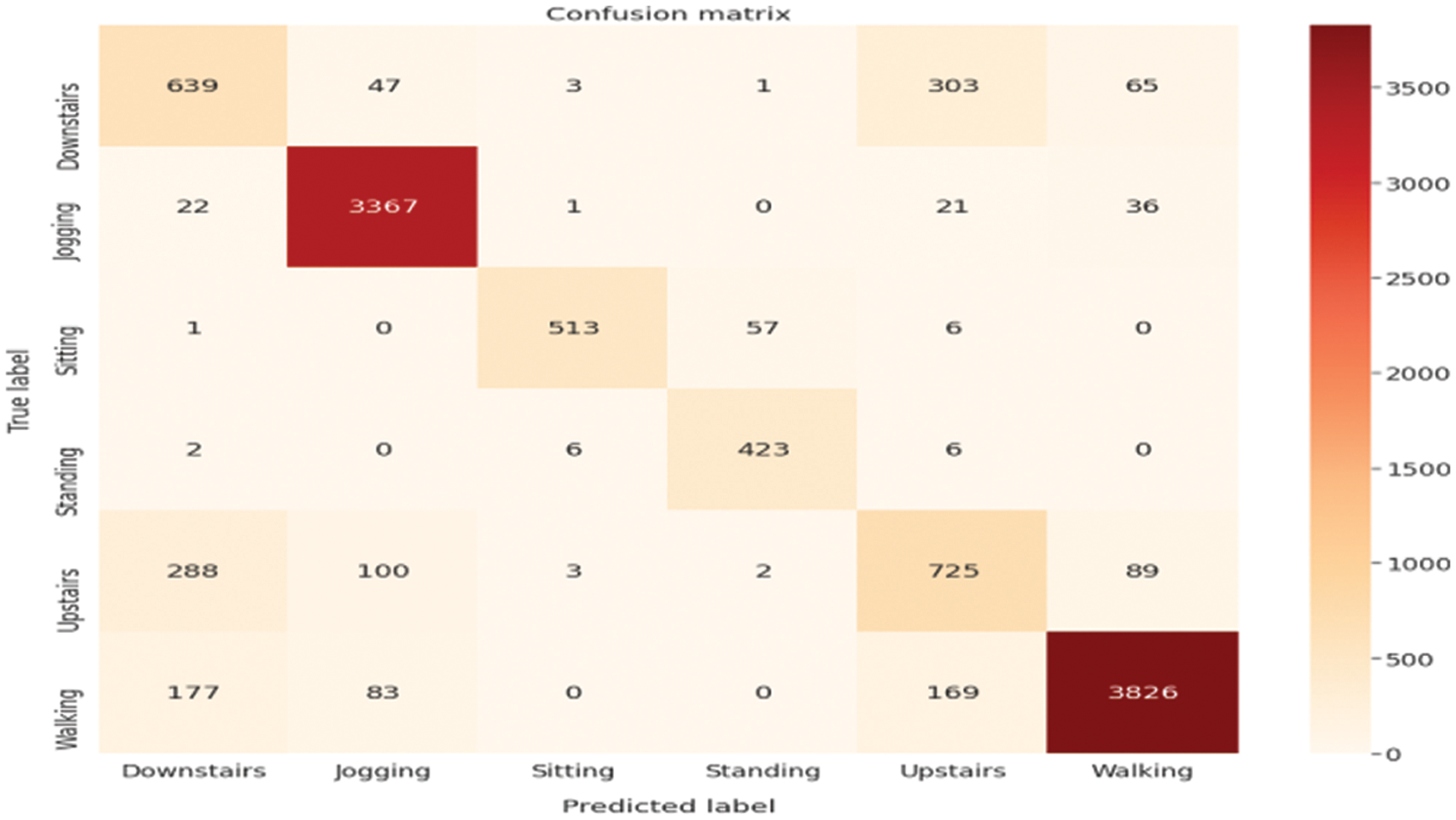
Figure 19: Confusion matrix for the LSTM model

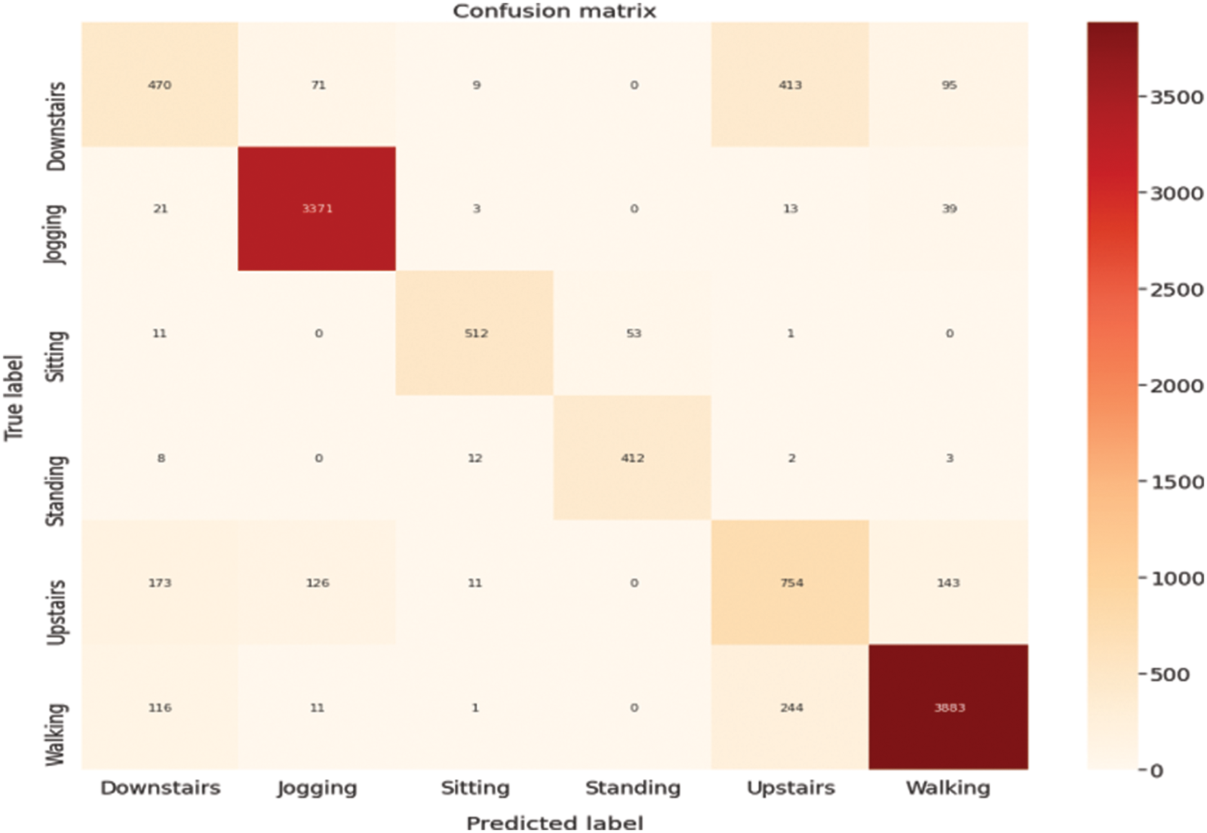
Figure 20: Confusion matrix for Bi-LSTM model

All three confusion matrices indicate how many out of six classes-walking, running, upstairs, downstairs, sitting and standing have been correctly classified. One of them shows how much percentage of the whole sample for that particular activity is classified accurately.

The final result of the experiment is given in Table 3. The performance of the human activity recognition by using the three neural network model is analysed during the research. The objective of the whole project is to categorize our daily human activities into six classes-walking, running, upstairs, downstairs, sitting, and standing. The accuracy metrics are used to evaluate features. The fraction of successfully categorized classifications is determined by the accuracy of the performance.

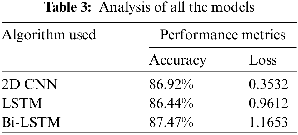
To understand the different neural network models and their importance to understand and recognize our daily routine-based human activities, tried out different approaches by using different models and pre-processing techniques in different algorithms and compared the results.

5.2 Comparisons

People with CP had a variety of predicted gait differences, including decreased stride length and speed, lower foot striking and lift-off pitch angles, and longer stance phases. As previously stated [39], our CP group’s gait speed was much lower. The overall accuracy and precision have been given in Table 4 and Fig. 21.

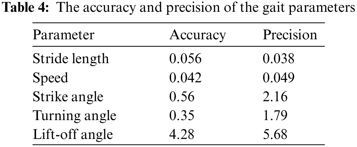
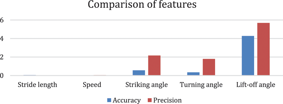
Figure 21: Comparison of accuracy and precision for gait features

Because gait cycle periods were simply marginally reduced in patients with CP, and without any major difference compared to controls, this was most likely due to decreased stride length. However, the large coefficient of variation, notably in the CP group, indicates a considerable inter-stride variability. The GMFCS (Gross Motor Function Classification System) level indeed appeared to be strongly linked with cadence, speed, and stride length [40]. The foot flatness period of posture has been demonstrated to improve the level of motor deficiency in persons with Parkinson’s disease with the help of inertial sensors. It demonstrated an improvement in posture and reduction in swinging phases in our subjects with CP using similar equipment as compared to healthy controls. Striking and elevator angles were dramatically reduced in paretic limbs, due to alterations in ankle kinematics caused by spasticity and subsequent contractures in the lower limbs. The average and difference of the parameters are plotted and shown in Fig. 22 below.

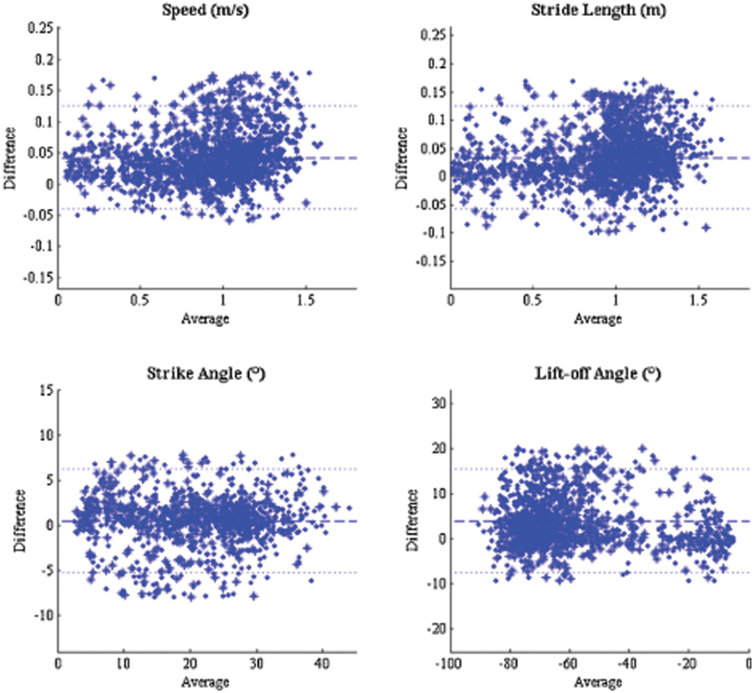
Figure 22: The plot of the difference and the average of the parameters

6  Conclusion

In this work, it has been demonstrated that recognizing daily routine-based human activities can be extremely accurate, with almost all activities accurately getting recognized over 90% of the time. Furthermore, because all the examples are generated from only 20 s of data, these actions can be recognized fast. Without the open-source WISDM (Wireless Sensor Data Mining) lab dataset which was provided by people from the lab on their website, this work would not have been possible. They had their WISDM (Wireless Sensor Data Mining) Android-based data gathering platform, which sends data from the phone to their Internet-based server, a valuable resource created as a result of their efforts. As a result of having this in place, it is capable of using their data and training the models efficiently so that it classified human activities accurately. According to the previous studies, the sensor is directly connected to the CNN (Convolution Neural Network) designed to generate ideas for small applications that are likely to keep open the implementation process on low-cost or embedded devices. The paper focuses more on the approaches taken for building the model to classify six activities. Some of the previous papers also tried to classify the models using non-neural network-based models i.e., machine learning models such as logistic regression and decision trees which learn from data and then make decisions, whereas in this case, it went with a complete neural network-based approach. In this approach, the network arranges itself in a way that it can make its own decisions that too with high accuracy. This research allowed investigating the variations in gait metrics in people with CP (Cerebral Palsy) during twisting and linear trajectory movements during turning, step width, stride length, and speed all decreased significantly as compared to straight gait. In addition, the gadget enabled to relate the features of motor behavior and adaption techniques in linear and rotating trajectories, indicating the greater importance of improved efficacy for people with CP (Cerebral Palsy) when rotating.

7  Future Work

Training the model can be done to recognize more activities such as bicycling, car-riding, etc. If such data is made available publicly as WISDM (Wireless Sensor Data Mining) lab dataset the work described and implemented in this project is part of a larger effort to classify human beings’ daily activities. It is planned to work on this project in the future to classify more such daily activities along with improvising on our existing work by improving the performance of the existing neural network-based classification models. It is believed that human activity recognition will play an important part in human-to-human interaction and interpersonal relationships since it delivers difficult-to-extract information or insight into a person’s identity, personality, and psychological condition. The gadgets, on the other hand, maybe simply calibrated in a flat-footed state of rest to allow for rectification of any fixed equines during gait.

Acknowledgement: The authors extend their hearty thanks to the WISDM Lab for providing the open-source data.

Funding Statement: The authors received no specific funding for this study.

Conflicts of Interest: The authors declare that they have no conflicts of interest to report regarding the present study.

References

1. L. Wang, Y. Sun, Q. Li, T. Liu and J. Yi, “IMU-based gait normalcy index calculation for clinical evaluation of impaired gait,” Journal of Biomedical and Health Informatics, vol. 25, no. 1, pp. 3–12, 2021. [Google Scholar]
2. Z. P. Luo, Z. Ping, J. Lawrence Berglund and K. Nan, “Validation of F-scan pressure sensor system: A technical note,” Journal of Rehabilitation Research and Development, vol. 35, pp. 186–186, 2017. [Google Scholar]
3. A. F. Bobick and J. W. Davis, “The recognition of human movement using temporal templates. Pattern analysis and machine intelligence,” IEEE Transactions on Pattern Analysis and Machine Intelligence, vol. 23, no. 4, pp. 257–267, 2009. [Google Scholar]
4. A. Stéphane, “Gait analysis in children with cerebral palsy,” European Federation of National Associations of Orthopaedics and Traumatology Open Reviews, vol. 1, no. 6, pp. 448–460. 2016. [Google Scholar]
5. L. Yao, W. Kusakunniran, Q. Wu, J. Zhang and Z. Tang, “Robust CNN-based gait verification and identification using skeleton gait energy image,” Digital Image Computing: Techniques and Applications (DICTA), vol. 5, pp. 1–7, https://doi.org/10.1109/DICTA.2018.8615802, 2018. [Google Scholar]
6. B. Mariani, M. C. Jimenez, F. J. Vingerhoets and K. Aminian, “On-shoe wearable sensors for gait and turning assessment of patients with Parkinson’s disease,” IEEE Transaction on Biomedical Engineering, vol. 60, no. 1, pp. 155–158, 2013. [Google Scholar]
7. S. C. Bakchy, M. R. Islam and A. Sayeed, “Human identification on the basis of gait analysis using kohonen self-organizing mapping technique,” in Proc. ICECTE, USA, pp. 1–4, 2016. [Google Scholar]
8. H. M. Rasmussen, N. W. Pedersen, S. Overgaard, L. K. Hansen, U. Dunkhase-Heinl et al., “Gait analysis for individually tailored interdisciplinary interventions in children with cerebral palsy: A randomized controlled tria,” Dev. Med. Child Neurol., vol. 61, no. 1, pp. 1189–1195, 2019. [Google Scholar]
9. B. Mariani, C. Hoskovec, S. Rochat, C. Bula and J. Penders, “3D gait assessment in young and elderly subjects using foot-worn inertial sensors,” Journal of Biomechanics, vol. 43, no. 15, pp. 257–267, 2010. [Google Scholar]
10. L. T. Kozlowski and J. E. Cutting, “Recognizing the sex of a walker from a dynamic point-light display,” Perception and Psychophysics, vol. 21, no. 6, pp. 575–580, 1977. [Google Scholar]
11. J. R. Kwapisz, G. M. Weiss and S. A. Moore, “Activity recognition using cell phone accelerometers,” ACM SigKDD Explorations Newsletter, vol. 12.2, pp. 74–82, 2011. [Google Scholar]
12. R. Polana and R. Nelson, “Detecting activities,” in Proc. CVPA, San Juan, PR, USA, vol. 7, pp. 2–7, 1993. [Google Scholar]
13. P. G. Rosquist, G. Collins, A. J. Merrell, N. J. Tuttle, J. B. Tracy et al., “Estimation of 3D ground reaction force using nanocomposite piezo-responsive foam sensors during walking,” Annals of Biomedical Engineering, vol. 45, no. 9, pp. 2122–2134, 2017. [Google Scholar]
14. R. Cutler and L. Davis, “Robust real-time periodic motion detection, analysis, and applications,” IEEE Transactions on Pattern Analysis and Machine Intelligence, vol. 22, no. 8, pp. 781–796, 2000. [Google Scholar]
15. S. Zihajehzadeh and E. J. Park, “Experimental evaluation of regression model-based walking speed estimation using lower body-mounted IMU,” in Proc. EMBC, Orlando, pp. 243–246, 2016. [Google Scholar]
16. S. Grad and E. J. Lawrence, “Movement speed estimation based on foot acceleration patterns,” in Proc. ENBC, Honolulu, HI, pp. 3505–3508, 2018. [Google Scholar]
17. N. Sazonova, R. C. Browning and E. Sazonov, “Accurate prediction of energy expenditure using a shoe-based activity monitor,” Medicine Science Sports and Exercise, vol. 43, no. 7, pp. 1312–1321, 2011. [Google Scholar]
18. J. Parkka, M. Ermes, P. Korpipaa, J. Mantyjarvi, J. Peltola et al., “Activity classification using realistic data from wearable sensors,” IEEE Transactions on Information Technology in Biomedicine, vol. 10, no. 1, pp. 119–128, 2006. [Google Scholar]
19. V. Bianchi, M. Bassoli, G. Lombardo, P. Fornacciari, M. Mordonini et al., “IoT wearable sensor and deep learning: An integrated approach for personalized human activity recognition in a smart home environment,” IEEE Internet of Things Journal, vol. 6, no. 5, pp. 8553–8562, 2019. [Google Scholar]
20. Z. Li, W. Chen, J. Wang and J. Liu, “An automatic recognition system for patients with movement disorders based on wearable sensors,” in Proc. ICIEA, Hainan, China, pp. 1948–1953, 2014. [Google Scholar]
21. G. Johansson and J. Liu, “Visual motion perception. Scientific American,” IEEE Transactions on Pattern Analysis and Machine Intelligence, vol. 23, pp. 257–267, 2010. [Google Scholar]
22. J. E. Cutting, D. R. Proffitt and L. T. Kozlowski, “A biomechanical invariant for gait perception,” Journal of Experimental Psychology: Human Perception and Performance, vol. 4, no. 3, pp. 357–372, 1978. [Google Scholar]
23. D. Tao, X. Li, X. Wu and S. J. Maybank, “General tensor discriminant analysis and gabor features for gait recognition,” IEEE Transactions on Pattern Analysis and Machine Intelligence, vol. 29, no. 10, pp. 1700–1715, 2007. [Google Scholar]
24. H. Zhao, P. Karlsson, O. Kavehei and A. McEwan, “Augmentative and alternative communication with Eye-gaze technology and augmented reality: Reflections from engineers, people with cerebral palsy and caregivers,” IEEE Sensors, vol. 9, no. 10, pp. 1–4, 2021. [Google Scholar]
25. B. Nguyen-Thai, C. Morgan, N. Badawi, T. Tran and S. Venkatesh, “A spatio-temporal attention-based model for infant movement assessment from videos,” IEEE Journal of Biomedical and Health Informatics, vol. 25, no. 10, pp. 3911–3920, Oct. 2021. [Google Scholar]
26. G. C. Burdea, D. Cioi, A. Kale, W. E. Janes, S. A. Ross et al., “Robotics and gaming to improve ankle strength, motor control, and function in children with cerebral palsy—A case study series,” IEEE Transactions on Neural Systems and Rehabilitation Engineering, vol. 21, no. 2, pp. 165–173, 2013. [Google Scholar]
27. R. T. Lauer, B. T. Smith and R. R. Betz, “Application of a neuro-fuzzy network for gait event detection using electromyography in the child with cerebral palsy,” IEEE Transactions on Biomedical Engineering, vol. 52, no. 9, pp. 1532–1540, 2005. [Google Scholar]
28. J. Kamruzzaman and R. K. Begg, “Support vector machines and other pattern recognition approaches to the diagnosis of cerebral palsy gait,” IEEE Transactions on Biomedical Engineering, vol. 53, no. 12, pp. 2479–2490, 2006. [Google Scholar]
29. M. J. O’Malley, M. F. Abel, D. L. Damiano and C. L. Vaughan, “Fuzzy clustering of children with cerebral palsy based on temporal-distance gait parameters,” IEEE Transactions on Rehabilitation Engineering, vol. 5, no. 4, pp. 300–309, 1997. [Google Scholar]
30. P. Andrade, B. E. Pinos-Velez and P. Ingavelez-Guerra, “Wireless transmitter of basic necessities for children with cerebral palsy,” in Proc. ISSE, Rome, Italy, pp. 420–424, 2015. [Google Scholar]
31. M. Wagner, D. Slijepcevic, B. Horsak, A. Rind, M. Zeppelzauer et al., “KAVAGait: Knowledge-assisted visual analytics for clinical gait analysis,” IEEE Transactions on Visualization and Computer Graphics, vol. 25, no. 3, pp. 1528–1542, 1 2019. [Google Scholar]
32. S. Springer and G. Seligman, “Validity of the kinect for gait assessment: A focused review,” Journal of Medical Engineering, vol. 16, pp. 194, 2016. [Google Scholar]
33. T. Hirotomi, Y. Iwasaki and A. Waller, “Assessing quality of movement in a child with cerebral palsy by using accelerometers,” in Proc. CME, Zhongshan, China, vol. 2, no. 16, pp. 750–753, 2012. [Google Scholar]
34. P. Garg, H. Sabnani, M. Maheshwari, R. Bagree and P. Ranjan, “CePal: An InfraRed based remote control for cerebral palsy patients,” in 2010 Int. Symp. on Electronic System Design, USA, vol. 32, no. 6, pp. 153–157, 2010. [Google Scholar]
35. H. Su, W. Chen and W. Hong, “Human gait recognition based on principal curve component analysis,” 2006 6th World Congress on Intelligent Control and Automation, China, vol. 2, no. 4, pp. 10270–10274, 2006. [Google Scholar]
36. L. Zhou and Y. Iwasaki, “Validation of an IMU gait analysis algorithm for gait monitoring in daily life situations,” in Proc. EMBC, Mexico, vol. 5, no. 2, pp. 4229–4232, 2020. [Google Scholar]
37. T. K. Bajwa, S. Garg and K. Saurabh, “Gait analysis for identification by using SVM with K-NN and NN techniques,” in Proc. PDGC, Waknaghat, Solan, Himachal Pradesh, pp. 259–263, 2016. [Google Scholar]
38. K. Monica and R. Parvathi, “Hybrid FOW—A novel whale optimized firefly feature selector for gait analysis,” Personal and Ubiquitous Computing, pp. 1–13, https://doi.org/10.1007/s00779-021-01525-4, 2021. [Google Scholar]
39. A. K. Seifert, M. G. Amin and A. M. Zoubir, “Toward unobtrusive inhome gait analysis based on radar micro-Doppler signatures,” IEEE Transactions on Biomedical Engineering, vol. 66, no. 9, pp. 2629–2640, 2019. [Google Scholar]
40. Y. Long, X. Chen and J. Xu, “Application of gait factor in reducing gait interferences,” in Proc. IHMSC, Hangzhou, China, vol. 6, no. 3, pp. 103–107, 2015. [Google Scholar]
Cite This Article
Copyright © 2023 The Author(s). Published by Tech Science Press.
This work is licensed under a Creative Commons Attribution 4.0 International License , which permits unrestricted use, distribution, and reproduction in any medium, provided the original work is properly cited.
Downloads
Citation Tools